Enhancing Quadrotor Control Robustness with Multi-Proportional–Integral–Derivative Self-Attention-Guided Deep Reinforcement Learning

Abstract

Deep reinforcement learning has demonstrated flexibility advantages in the control field of quadrotor aircraft. However, when there are sudden disturbances in the environment, especially special disturbances beyond experience, the algorithm often finds it difficult to maintain good control performance. Additionally, due to the randomness in the algorithm’s exploration of states, the model’s improvement efficiency during the training process is low and unstable. To address these issues, we propose a deep reinforcement learning framework guided by Multi-PID Self-Attention to tackle the challenges in the training speed and environmental adaptability of quadrotor aircraft control algorithms. In constructing the simulation experiment environment, we introduce multiple disturbance models to simulate complex situations in the real world. By combining the PID control strategy with deep reinforcement learning and utilizing the multi-head self-attention mechanism to optimize the state reward function in the simulation environment, this framework achieves an efficient and stable training process. This experiment aims to train a quadrotor simulation model to accurately fly to a predetermined position under various disturbance conditions and subsequently maintain a stable hovering state. The experimental results show that, compared with traditional deep reinforcement learning algorithms, this method achieves significant improvements in training efficiency and state exploration ability. At the same time, this study deeply analyzes the application effect of the algorithm in different complex environments, verifies its superior robustness and generalization ability in dealing with environmental disturbances, and provides a new solution for the intelligent control of quadrotor aircraft.

1. Introduction

Drone technology has become a hot topic in recent years. As a remotely controlled flight device, drones have shown wide applications in various fields such as military, civilian, and commercial fields, including reconnaissance, strikes, transportation, aerial photography, express delivery, advertising, entertainment, and film and television [1,2]. However, traditional drone control strategies mainly rely on fixed rules and policies, which may be effective in specific situations but have limited adaptability in complex and variable real-world environments. For example, under strong winds or extreme weather conditions, traditional control strategies may fail to ensure the stable flight of drones. As the complexity of tasks increases, such as precise reconnaissance in urban environments, the requirements for drone control systems are also increasing.

Through continuous interaction with the environment, deep reinforcement learning (DRL) algorithms can self-learn and optimize the control strategies of drones, thus adapting to various tasks and improving performance in dynamic environments [3,4]. However, in practical applications, DRL algorithms still face some challenges, especially in environments with abrupt factors. The low training efficiency of the model and its difficulty in coping with unprecedented abrupt factors limit the practicability of DRL algorithms in the field of drone control.

Currently, reinforcement learning faces the following challenges in the field of drone control:

C1. Environmental uncertainty and dynamics: Drones need to fly under various changing conditions, such as climate changes and the appearance of obstacles. These factors can affect the flight status of drones, and reinforcement learning models must be able to cope with this environmental uncertainty and dynamics.

C2. Training efficiency issues: Reinforcement learning usually requires a large number of interaction samples to train the model. However, in the actual drone training process, once a local optimum is reached and there is no good random exploration strategy, it can easily result in drones requiring significant amounts of exploration and training, seriously reducing the training efficiency.

C3. Model robustness issues: In reinforcement learning for drone control, the stability and reliability of the control strategy under model errors and external interferences must be considered. Solving this problem is crucial for improving the safety and reliability of autonomous drone flight.

This study constructs a simulation model of a quadrotor drone and a simulation environment with environmental disturbances to address C1. Additionally, a Multi-PID Self-Attention guidance module is proposed to tackle C2 and C3. This algorithm integrates PID (Proportional–Integral–Derivative) control [5] strategies into the basic framework of deep reinforcement learning to optimize the state reward function in the simulation environment. Leveraging a multi-head self-attention mechanism, an efficient training guidance module is constructed. By introducing multiple disturbance models to simulate complex real-world scenarios, a disturbed simulation experiment environment is established. In this simulation environment, the efficiency and robustness of the proposed algorithm are validated. In summary, we have made the following contributions:

• We propose a Multi-PID Self-Attention guidance module that combines PID control strategies and a multi-head self-attention mechanism. This module optimizes the state reward function in the simulation environment based on the fundamental architecture of deep reinforcement learning. During the training process, this module can effectively guide the training, improve exploration efficiency and stability, and reach a state of higher rewards faster, thus avoiding falling into local optima due to random exploration and the difficulty of recovery.
• By introducing random Gaussian white noise interference into the training environment, the trained model exhibits significant robustness and performs well in various interference environments within the simulation experiment environment. Specifically, it demonstrates superior performance compared to the original model when encountering step-like disturbances.

The structure of this paper is as follows: Section 2 reviews the applications and advancements of reinforcement learning in unmanned aerial vehicle (UAV) control; Section 3 outlines the research framework, including the design of the PID controller, self-attention module, and environmental disturbances; Section 4 details the principles of benchmark algorithms (A2C [6], SAC [7], PPO-Clip [8]) and the guiding module, as well as the modeling of environmental disturbances; Section 5 introduces the construction of the simulation environment, including functional components and the quadrotor model; Section 6 evaluates the performance of the reinforcement learning flight controller through experiments; finally, the research findings are summarized, and future directions are discussed.

2. Related Work

2.1. Drone Simulation and Reinforcement Learning Environment

With the rapid development of drone technology, how to build an efficient and realistic simulation environment and how to use reinforcement learning technology to optimize the control strategy of drones have become research hotspots.

Zhao [9] emphasized that the differences between simulation and reality can potentially affect the performance of strategies in actual robots. The current research focuses on minimizing the sim-to-real gap and exploring effective policy transfer. Kang [10] proposed a learning method that combines real-world and simulation data, utilizing real data to learn system dynamics and training a generalizable perception system with simulation data. Mahmud [11] aimed to enhance the performance of non-orthogonal multiple access drone (NOMA-UAV) networks and demonstrated significant improvements in total rate, rate outage probability, and average bit error rate through simulation experiments. Bekar [12] developed a drone control system design method that combines high-fidelity models and incremental reinforcement learning, enabling adaptation to changing operating conditions and allowing for realistic simulation testing in a virtual reality environment. Koch [13] created a reinforcement learning (RL) training simulation environment for drone flight control and explored the potential of RL for the inner-loop control of drones, comparing it to traditional PID controllers.

As technology continues to advance, the research pertaining to the UAV simulation and reinforcement learning environment is poised to further intensify, thereby offering a more robust theoretical underpinning and practical foundation for the progression of UAV technology.

2.2. Intelligent Control for Drones

In optimizing UAV control strategies, researchers aim to improve the autonomous navigation and trajectory tracking capabilities of drones by introducing various methods such as deep learning, genetic algorithms, and fuzzy logic.

Guo [14] designed a distributed deep reinforcement learning framework that divides the UAV navigation task into two simpler subtasks, each handled by a specifically tailored LSTM-based DRL network. This framework also cleverly utilizes partial interaction data to improve the efficiency of the training process and resource utilization. Cavanini [15] developed an MPC autopilot for a specific UAV weather data sampling task and demonstrated the performance of its control strategy through algorithm comparisons. Siti [16] proposed two PD/PID-based trajectory tracking strategies and optimized the controller parameters using genetic algorithms, significantly improving the trajectory tracking capability of quadrotor drones in complex environments. Kurnaz [17] constructed a fuzzy logic-based UAV navigation controller and evaluated and verified its performance in various simulation environments, demonstrating its potential and effectiveness in achieving autonomous navigation for UAVs. Din [18] proposed an intelligent control architecture based on reinforcement learning, specifically model-free RL techniques, to address UAV control problems and proved its effectiveness and superiority under different environmental conditions through simulations. The PPF-based fixed-wing UAV formation path planning method proposed by Fang [19] overcomes local optimality and smoothness issues via virtual potential field vectors and dynamic adjustments. PPSwarm introduced by Meng [20] combines RRT* and PSO to tackle fast convergence and local optimality in multi-UAV path planning. The Transformer architecture, widely used in sequential data processing, handles long-distance dependencies efficiently. The ContextAD method developed by Ou [21], leveraging the Transformer and self-attention, improves abbreviation disambiguation accuracy and robustness by fusing contextual information. Wang [22] developed a DRL method suitable for UAV navigation in large-scale complex environments and demonstrated its effectiveness and superiority through experiments. Bayerlein [23] applied reinforcement learning to trajectory optimization for UAV base stations and trained the UAV to make optimal movement decisions autonomously using Q-learning, thus improving the overall system performance. Rodriguez-Ramos [24] applied deep reinforcement learning algorithms to UAV landing tasks and verified their effectiveness through simulation training and real-world flight tests. Wang [25] proposed a new safe RL method based on soft obstacle functions that can effectively handle hard safety constraints and showed excellent system safety in simulations. Zhang [26] developed a hierarchical control strategy suitable for the formation flight of multi-rotor drones and validated it through actual flight tests.

The optimization of UAV control strategies and the development of intelligent control architectures provide more possibilities for drones to achieve autonomous navigation and trajectory tracking in complex environments. With the continuous advancement of technology, drones will demonstrate their unique advantages and application value in more fields. Currently, the field of UAV control strategy optimization is pursuing more efficient, intelligent, and flexible flight control with the aid of advanced algorithms such as deep reinforcement learning. However, existing simulation environments have deficiencies in simulating real-world environmental interferences, resulting in insufficiently comprehensive evaluations of control effects. Especially when facing step-type disturbances, the robustness of the model becomes crucial. Therefore, improving the robustness of existing algorithms to cope with complex and variable real-world environments has become an important research direction.

3. Framework

To significantly enhance the robustness of deep reinforcement learning algorithms, this paper introduces the PID control method, which can evaluate the state of the aircraft in real-time and dynamically adjust the learning reward of the algorithm based on this evaluation, effectively guiding the model’s learning process. Compared to traditional training strategies, this new approach significantly improves training efficiency. However, we also observed that the algorithm’s performance is often influenced by the choice of PID parameters in different parts of the flight scenario. To overcome this parameter sensitivity issue, we incorporated a multi-head self-attention module that can concurrently evaluate multiple PID controllers with different parameters and dynamically generate reward values based on these evaluations. This mechanism effectively reduces the algorithm’s sensitivity to PID parameter settings, thereby enhancing its adaptability in variable environments. Additionally, to further improve the model’s robustness in complex and disturbed environments, we introduced random Gaussian white noise disturbances into the training environment. This measure allows the model to accumulate experience in handling abnormal disturbances during the training process, thereby demonstrating more robust performance when facing unknown disturbances in real-world environments.

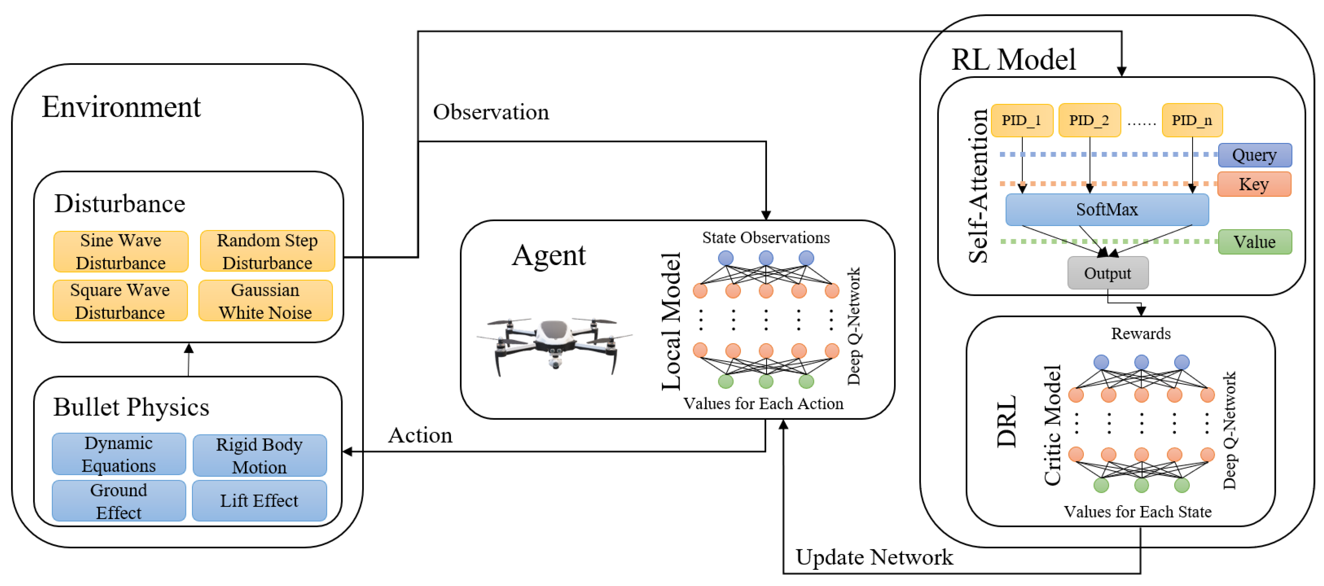
This section outlines the overall architecture of the current study, as illustrated in Figure 1. The research adopts the DRL algorithms as the baselines and incorporates a Multi-PID Self-Attention guidance module to improve its training process. Unlike previous approaches, we do not treat the PID controller as a control method; instead, we use it as an evaluation metric for the performance of the reinforcement learning model, guiding the training process accordingly. Additionally, a self-attention mechanism is introduced to integrate the outputs of multiple controller variants. This allows the framework to learn the control preferences of these controllers rather than their specific parameter details, thereby avoiding reliance on particular parameter settings. During each round of simulation training, the policy model conducts random exploration based on the results from the previous round. The self-attention mechanism dynamically evaluates the outputs of multiple controllers throughout the training process. By increasing focus on poorly performing controllers, it effectively prevents the agent from deviating from the optimal state due to consecutive poor random explorations. This approach avoids local optima, ensuring the stability of the entire training process. During the agent’s interaction with the environment, several types of disturbances are introduced. Gaussian white noise is employed during training to optimize decision-making under uncertain conditions. To validate the training effectiveness, the agent’s performance is observed under three additional types of disturbances and Gaussian white noise with different random seeds, testing the robustness of the trained control model.

4. Technical Details

In this section, we will utilize the DRL algorithms as the baselines for our study. We will provide a detailed description of the steps of the DRL algorithms improved by the Multi-PID Self-Attention module and introduce the interference pattern characteristics of several disturbance types in the experimental environment.

4.1. RL Module

4.1.1. A2C

A2C (Advantage Actor–Critic) combines the advantages of policy gradient and value function methods. It outputs a policy through an actor network, which provides the probability distribution of selecting each action given a state. Simultaneously, a critic network estimates the state-value function or state-action value function. A2C uses the advantage function to reduce the variance in policy gradient estimates, thereby enhancing training stability and sample efficiency.

In the A2C algorithm, a trajectory is first sampled from the environment, recording the states, actions, rewards, and next states. Then, the advantage function values are calculated using the critic network. These advantage values are used to update the actor network parameters, optimizing the policy towards increasing expected returns. Simultaneously, the critic network updates its parameters by minimizing the temporal difference (TD) error. The main advantages of A2C are the high sample efficiency and good training stability. However, it has high computational complexity, requiring the training of two networks, and involves complex hyperparameter tuning.

The implementation process of the A2C algorithm primarily includes the following steps:

• Calculating the Advantage Function:
  Use the critic network to estimate the state values $V\left(s_t\right)$ and $V\left(s_{t+1}\right)$ to compute the advantage function value.

  $$\begin{array}{c}\mathrm{A}\left(s_t,a_t\right)=r_t+\gamma \mathrm{V}\left(s_{t+1}\right)-\mathrm{V}\left(s_t\right)\end{array}$$

  (1)

  where $r_t$ is the reward, $s_t$ is the state, $a_t$ is the action, $s_{t+1}$ is the next state, and $\gamma$ is the discount factor hyperparameter.
• Update the Actor Network:
  Use the advantage function values to update the actor network parameters $\theta$ according to the policy gradient formula.

  $$\begin{array}{c}\theta =\theta +\alpha {\nabla }_{\theta }\log \pi (a_t|s_t,\theta )\mathrm{A}\left(s_t,a_t\right)\end{array}$$

  (2)

  where $\alpha$ is the learning rate hyperparameter.
• Update the Critic Network:
  Minimize the temporal difference (TD) error to update the critic network parameters $\varphi$.

  $$\begin{array}{c}\varphi =\varphi -\beta {\nabla }_{\varphi }{\mathrm{A}}^2\left(s_t,a_t\right)\end{array}$$

  (3)

  where $\beta$ is the learning rate hyperparameter.

Algorithm 1 presents the specific implementation process of the A2C algorithm. In line 1, the parameters of the action network, critic network, discount factor, and learning rate are initialized. Lines 3 to 15 constitute the main loop of the algorithm. Line 4 represents the collection of trajectory data using the current policy. Lines 6 compute the advantage function. Line 8 normalizes the advantage function. Lines 9 to 14 form the inner loop, which performs multiple training updates on each batch, including calculating the policy loss and value loss and updating the action network and critic network parameters using gradient ascent and gradient descent methods. Finally, line 17 outputs the updated actor network.

Algorithm 1: A2C: Advantage Actor–Critic
1	Initialization: action network parameters $\theta$, critic network parameters $\varphi$, discount factor $\gamma$, learning rates $\alpha$ and
2	$\beta$
3	for $iteration\leftarrow 1\mathrm{to}{T}_{iterations}$ do:
4	Collect trajectory $T$ using policy ${\pi }_{\theta }$.
5	for each step in trajectory $T$ do:
6	Compute advantage $\mathrm{A}\left(s_t,a_t\right)$ using Equation (1).
7	end for
8	Normalize advantages $\mathrm{A}\left(s_t,a_t\right)$.
9	for $epoch\leftarrow 1 to N_{epochs}$ do:
10	for $batch\leftarrow 1 to N_{mini\_batches}$ do:
11	Compute policy loss and update action network parameters θ using Equation (2).
12	Compute value loss and update critic network parameters w using Equation (3).
13	end for
14	end for
15	Update actor network $\pi \leftarrow {\pi }_{\theta }$.
16	end for
17	Output: Updated actor network $\pi$.

4.1.2. SAC

SAC (Soft Actor–Critic) is an entropy-based reinforcement learning algorithm designed to optimize both the expected return and the entropy of the policy, encouraging stochasticity to enhance exploration capabilities. SAC employs dual value networks to estimate the state-action value function $Q\left(s,a\right)$, reducing the bias in value function estimation. It also introduces a temperature parameter to automatically adjust the weight of policy entropy, balancing exploration and exploitation. This design enables SAC to perform well in high-dimensional continuous-action spaces, making it suitable for complex tasks.

The SAC algorithm process involves sampling a trajectory from the environment, using the critic networks to estimate the state-action value function and compute target values, then updating the critic network parameters. Next, the actor network parameters are updated to maximize both the expected return and the entropy of the policy. Finally, the temperature parameter is adjusted to meet the current exploration needs of the policy. Despite its higher computational complexity, requiring the training of multiple networks and the potential difficulty in tuning the temperature parameter, SAC’s strong exploration capability and adaptability to complex tasks have made it widely popular in practice.

The implementation process of the SAC algorithm primarily includes the following steps:

• Calculate Target Value:

  $$\begin{array}{c}y=r_t+\gamma Q_{target}\left(s_{t+1},a_{t+1}\right)-\alpha \log \pi \left(a_{t+1 }|s_{t+1 }\right)\end{array}$$

  (4)

  where $Q_{target}$ is the output of the target Q-network, $\alpha$ is the temperature parameter, and $\pi$ is the policy.
• Update Critic Network:
  Minimize the loss functions of the two critic networks to update critic network parameters ${\varphi }_1$ and ${\varphi }_2$.

  $$\begin{array}{c}{\varphi }_i={\varphi }_i-\beta {\nabla }_{{\varphi }_i}{\left(Q_{{\varphi }_i}\left(s_t,a_t\right)-y\right)}^2\end{array}$$

  (5)

• Update Actor Network:
  Maximize the weighted sum of the expected return and the entropy of the policy to update actor network parameters $\theta$.

  $$\begin{array}{c}\theta =\theta +\alpha {\nabla }_{\theta }\{{\mathrm{E}}_{{\mathrm{a}}_{\mathrm{t}}~{\varphi }_{\theta }}[\min \left(Q_{{\varphi }_1}\left(s_t,a_t\right),Q_{{\varphi }_2}\left(s_t,a_t\right)\right)-\mathsf{\alpha }\log \pi (a_t|s_t,\theta )]\}\end{array}$$

  (6)
• Update Temperature Parameter:
  Adjust the temperature parameter $\alpha$ by minimizing the entropy loss of the policy.

  $$\begin{array}{c}\alpha =\alpha +\beta {\nabla }_{\alpha }\left(\log \pi \left(a_t|s_t\right)-\widehat{H}\right)\end{array}$$

  (7)

  where $\widehat{H}$ is the target entropy.

Algorithm 2 presents the specific implementation process of the SAC algorithm. In line 1, the parameters for the policy network, two Q-networks, the target Q-network, and the temperature parameter are initialized. Lines 3 to 14 constitute the main loop of the algorithm. Line 4 represents the collection of trajectory data using the current policy. Lines 6 to 8 compute the target value. Line 9 calculates and updates the loss for the Q-networks. Line 10 calculates and updates the policy loss. Line 11 calculates and updates the temperature loss. Line 12 performs a soft update of the target Q-network parameters. Finally, line 16 outputs the updated policy network, Q-networks, and temperature parameter.

Algorithm 2: SAC: Soft Actor–Critic
1	Initialization: policy network parameters $\theta$, two Q-network parameters ${\varphi }_1$ and ${\varphi }_2$, target Q-network
2	parameters ${\varphi }_{target\_1}$ and ${\varphi }_{target\_2}$, temperature parameter $\alpha$.
3	for $iteration\leftarrow 1\mathrm{to}{T}_{iterations}$ do:
4	Collect trajectory $T$ using policy ${\pi }_{\theta }$.
5	for each step in trajectory $T$ do:
6	Sample action $a_t$ using policy ${\pi }_{\theta }$.
7	Observe reward $r_t$ and next state $s_{t+1}$.
8	Compute target value$y$ using Equation (4).
9	Compute Q-network losses and update Q-network parameters ${\varphi }_1$ and ${\varphi }_2$ using Equation (5).
10	Compute policy loss and update policy network parameters $\theta$ using Equation (6).
11	Compute temperature loss and update temperature parameter $\alpha$ using Equation (7).
12	Soft     update target Q-network parameters ${\varphi }_{target\_1}$ and ${\varphi }_{target\_2}$: ${\varphi }_{target\_i}\leftarrow \alpha \ast {\varphi }_1+\left(1-\alpha \right)\ast {\varphi }_{target\_i}$
13	end for
14	Update policy network $\pi \leftarrow {\pi }_{\theta }$.
15	end for
16	Output: Updated policy network $\pi$.

4.1.3. PPO-Clip

In traditional policy gradient methods, the update of policy parameters typically relies on some form of gradient ascent, aiming to maximize the accumulated reward. However, this update approach can lead to drastic changes in policy parameters, resulting in instability and convergence difficulties during the training process. Proximal Policy Optimization (PPO) employs an innovative objective function that effectively constrains policy changes during policy updates. By controlling the KL (Kullback–Leibler) divergence between the new and old policies, PPO ensures that the magnitude of policy updates is appropriate, maintaining both policy stability and convergence. This mechanism effectively avoids potential drastic oscillations during policy updates, significantly improving the stability and training efficiency of the algorithm.

To further constrain the magnitude of policy updates, the PPO algorithm introduces a clipping mechanism. Specifically, the algorithm utilizes a clipping function to limit the change in policy parameters between updates within a predefined range. This clipping mechanism effectively prevents excessive adjustments to policy parameters, ensuring the stability of the update process and effectively avoiding gradient explosion or disappearance issues. The application of the clipping function not only maintains the continuity of the policy but also improves the convergence speed and control accuracy of the algorithm.

The implementation process of the PPO-Clip algorithm mainly includes the following steps:

• Calculating the Advantage Function:
  The advantage function represents the advantage of taking a certain action in each state compared to the average action.

  $$\begin{array}{c}{V}_{pred}=valu{e}_{network}\left(s\right)\end{array}$$

  (8)

  $$\begin{array}{c}{L}_v\left(w\right)=\mathrm{MSE}\left(V_{pred},V_{target}\right)\end{array}$$

  (9)

  where $V_{pred}$ is the predicted state-value function under a given state $s$, $V_{target}$ is the target value function, which is typically calculated based on the discounted returns of collected rewards, and $\mathrm{MSE}\left(\cdot \right)$ is the mean squared error function used to compute the loss of the value function.
• Calculating the Policy Loss Function:
  The policy loss function in PPO-Clip consists of two components: one is a loss term based on the advantage function, which optimizes the policy to maximize the expected cumulative reward.

  $$\begin{array}{c}{\pi }_{ratio}=\frac{{\pi }_{new}\left(a|s\right)}{{\pi }_{old}\left(a|s\right)}\end{array}$$

  (10)

  $$rati{o}_{clipped}=\mathrm{clip}\left({\pi }_{ratio},1-\epsilon ,1+\epsilon \right)$$

  (11)

  $$surrogate={\pi }_{ratio}\ast \mathrm{Ad}\left(s,a\right)$$

  (12)

  $$\begin{array}{c}surrogat{e}_{clipped}=rati{o}_{clipped}\ast Ad\left(s,a\right)\end{array}$$

  (13)

  where ${\pi }_{ratio}$ represents the ratio between the new policy and the old policy, $\epsilon$ is the threshold used for clipping the ratio, and $\mathrm{clip}\left(x, min, max\right)$ is a function that clips $x$ to the range $\left[min, max\right]$. ${\pi }_{new}(a|s)$ is the probability of acting a under the new policy given state $s$, and ${\pi }_{old}(a|s)$ is the probability of acting $a$ under the old policy given state $s$. $\mathrm{Ad}\left(s, a\right)$ is the value function of executing action $a$ in state $s$.
  The other part of the policy loss function is based on the ratio between the new and old policies, which is used to limit the magnitude of policy updates. Specifically, the policy loss function can be expressed as follows:

  $$\begin{array}{c}{L}_{policy}=-min\left(surrogate,surrogat{e}_{clipped}\right)\end{array}$$

  (14)

  $$\begin{array}{c}{L}_{total}=L_{policy}+c1\ast L_v\left(w\right)\end{array}$$

  (15)

  where $c1$ is a hyperparameter for the value loss, which is used to adjust the influence of the value loss on the total loss.

Algorithm 3 presents the detailed implementation process of the PPO-Clip algorithm. Line 1 of the code initializes the network parameters, clipping range, and hyperparameters. Lines 3 to 24 constitute the main loop of the algorithm, where Line 4 represents the collection of trajectory data using the current policy, and Lines 4 and 5 compute and normalize the advantage function. Lines 8 to 12 are the inner loop, which performs multiple training updates on each batch, including computing the surrogate objective, value loss, and total loss, and updating the parameters of the policy network and value network using gradient ascent and gradient descent methods. Finally, Line 17 outputs the updated policy network.

Algorithm 3: PPO-Clip: Proximal Policy Optimization with Clipping
1	Initialization: policy network parameters $\theta$, value network parameters $w$, clipping range $ϵ$, hyperparameters $c1$.
2	for $iteration\leftarrow 1\mathrm{to}{T}_{iterations}$ do:
3	Collect trajectory $T$ using policy ${\pi }_{\theta }$.
4	Compute advantages $\mathrm{Ad}\left(s, a\right)$ using value network.
5	Normalize advantages $\mathrm{Ad}\left(s, a\right)$.
6	for$epoch\leftarrow 1 to N_{epochs}$ do:
7	for $batch\leftarrow 1 to N_{mini\_batches}$ do:
8	Compute surrogate objective $surrogat{e}_{clipped}$ using Equation (13).
9	Compute value loss$L_v\left(w\right)$ using Equation (9).
10	Compute total loss $L_{total}$ using Equation (15).
11	Update policy network parameters $\theta$ using gradient ascent on $L_{total}$.
12	Update value network parameters $w$ using gradient descent on$L_v\left(w\right)$.
13	end for
14	end for
15	Update policy network $\pi \leftarrow {\pi }_{\theta }$.
16	end for
17	Output: Updated policy network $\pi$.

4.1.4. Multi-PID Self-Attention Module

1.

PID Reward Function:

The PID controller is a classical feedback control system widely used in various industrial control scenarios. It measures the deviation between the actual output of the system and the desired output and adjusts the output of the controller based on the magnitude of the deviation and its changing trend, thereby stabilizing the system output near the desired value.

The PID controller consists of three fundamental elements: proportional, integral, and derivative. These three elements correspond to three tuning parameters of the controller: the proportional coefficient ($K_p$), the integral time ($K_i$), and the derivative time ($K_d$).

The output of the PID controller is given by the following formula:

$$\begin{array}{c}u\left(t\right)=K_p\cdot e\left(t\right)+K_i\cdot {{\displaystyle \int }}_0^{t}e\left(\tau \right)d\tau +K_d\cdot \frac{de\left(t\right)}{dt} \end{array}$$

(16)

where $u\left(t\right)$ represents the controller output value at time t, which is the control signal. $e\left(t\right)$ is the system error at time t, which is the difference between the desired value and the actual value. $K_p$ is the proportional coefficient. $K_i$ is the integral coefficient. $K_d$ is the derivative coefficient.

The reward function $Q_t$ for each simulation step is defined as follows:

$$\begin{array}{c}{Q}_t=D-{\left[K_p\left(P_t-P_{target}\right)+K_i\int \left(P_t-P_{target}\right)dt+K_d\left(P_t-P_{t-1}\right)\right]}^2\end{array}$$

(17)

where $P_t$ represents the position of the aircraft at time t, and $P_{target}$ represents the target position. The upper bound of the reward, $D$, is defined as follows:

$$\begin{array}{c}D=2\Vert P_t-P_{target}\Vert \end{array}$$

(18)

2.

Multi-Head Self-Attention Module

Self-attention is a special type of attention mechanism where the Query, Key, and Value all come from the same input sequence. It allows each element in the sequence to interact with every other element in the sequence to compute a relevance score between them. This mechanism enables the model to capture long-range dependencies in the input sequence and perform exceptionally well when processing sequential data.

The implementation process of self-attention includes the following key steps:

• Calculation of Query, Key, and Value:
  For each element in the input sequence, three different linear transformations are used to compute its Query, Key, and Value vectors.

  $$\begin{array}{c}Query=Q_t\ast W_q\end{array}$$

  (19)

  $$\begin{array}{c}Key=Q_t\ast W_k\end{array}$$

  (20)

  $$\begin{array}{c}Value=Q_t\ast W_v\end{array}$$

  (21)

  where $Q_t$ represents the embedding vector matrix of the input sequence, and $W_q$, $W_k$, and $W_v$ are the linear transformation matrices used to compute the Query, Key, and Value vectors, respectively.
• Calculating Attention Scores:
  For each position in the sequence, its Query vector is dot-produced with the Key vectors of all positions in the sequence to obtain a series of attention scores. These scores represent the relevance between the current position and other positions.

  $$\begin{array}{c}score{s}_{attention}=\mathrm{softmax}\left(\frac{Query\cdot Key}{sqrt\left(d\right)}\right)\end{array}$$

  (22)

  where $d$ is the dimension of the Key vector, used to scale the dot-product attention scores to prevent gradient vanishing or exploding. The $\mathrm{softmax}\left(\cdot \right)$ function is then applied to normalize the attention scores into a probability distribution.
• Weighted Summation:
  Using the attention weights, the Value vectors at all positions in the sequence are weighted and summed to obtain the output representation for the current position. This output representation considers the information from all positions in the sequence, with emphasis on the parts most relevant to the current position.

  $$\begin{array}{c}reward=score{s}_{attention}\cdot Value\end{array}$$

  (23)

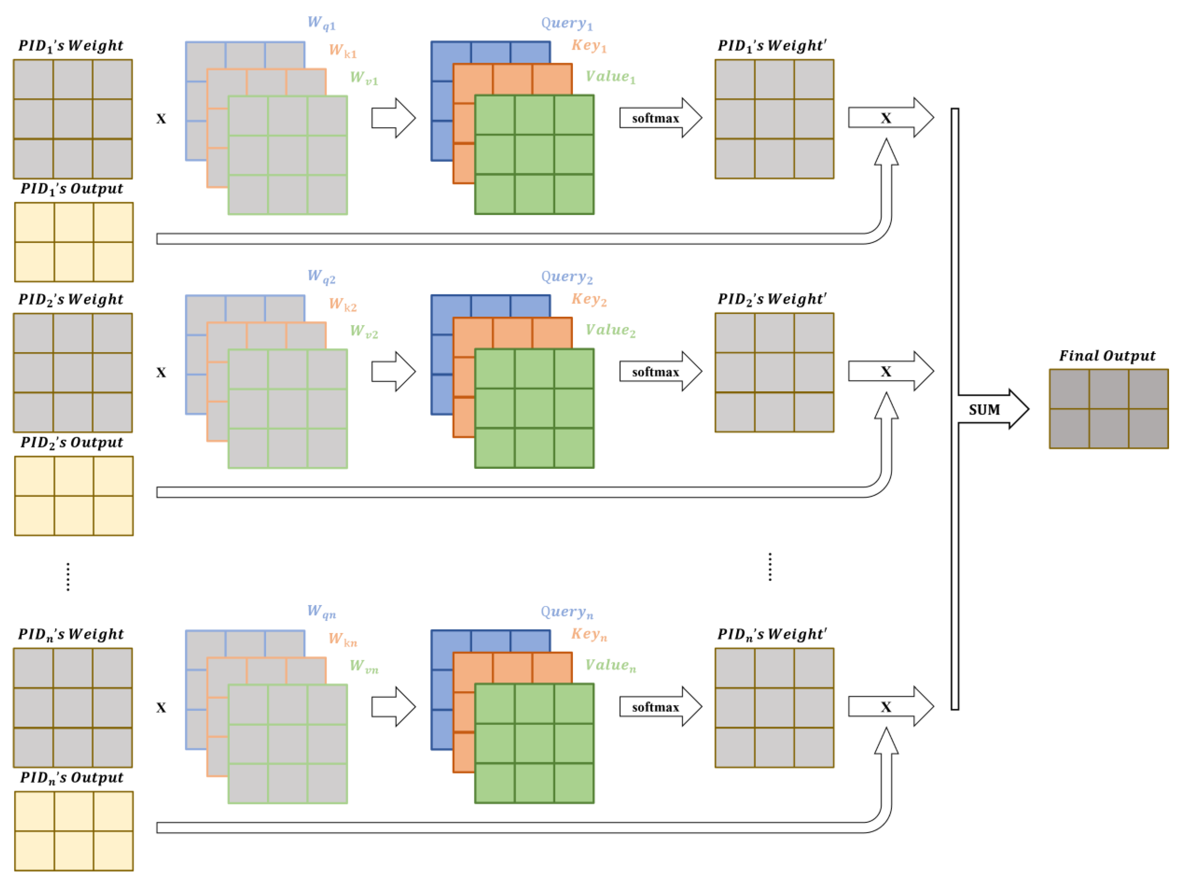
In scenarios where multiple output options are available, self-attention helps the model dynamically capture each system’s feedback on different options and focus on the aspects that are most beneficial for overall optimization. This effectively aids the model in selecting the optimal reward value, thereby enhancing the model’s update process. The design of the self-attention module in the framework is shown in Figure 2.

Algorithm 4 presents an enhanced DRL algorithm based on a Multi-PID Self-Attention mechanism. In Line 1 of the code, the DRL network, learnable parameter matrices $W_q, W_k, and W_v$, and PID controller parameters $\left(k_p, k_i, k_d\right)$ are initialized. Then, during each iteration, the simulation environment is first initialized. Next, for each epoch, the algorithm updates the DRL network $\pi$ on each mini-batch of data, using reward values calculated based on environmental feedback (like Line 11–12 in Algorithm 1, Line 6–12 in Algorithm 2, and Line 8–12 in Algorithm 3). After completing the network update, the algorithm calculates the output $Q_t$ of the PID controller. Subsequently, the algorithm utilizes the self-attention mechanism to dynamically capture the relevance of different system feedback by computing Query, Key, and Value matrices, as well as attention scores, and calculates a weighted sum of reward values. This process is repeated for multiple epochs and iterations to continuously optimize the policy network $\pi$. Finally, the algorithm outputs the updated policy network $\pi$.

Algorithm 4: Enhanced DRL based on Multi-PID Self-Attention
1	Initialization: the DRL network, Learnable parameter matrices $W_q, W_k, W_v$, PID parameter $\left(k_p, k_i, k_d\right)$.
2	for $iteration\leftarrow 1\mathrm{to}{T}_{iterations}$ do:
3	Initialize the simulation environment.
4	for$epoch\leftarrow 1 to N_{epochs}$ do:
5	Calculate PID controller output $Q_t$ using Equation (17).
6	Compute Query, Key, and Value matrices using Equation (21).
7	Compute attention scores $score{s}_{attention}$ using Equation (22).
8	Compute weighted sum $reward$ using Equation (23).
9	for $batch\leftarrow 1 to N_{mini\_batches}$ do:
10	Update DRL police network $\pi$ using $reward$.
11	// Line 11–12 in Algorithm 1, Line 6–12 in Algorithm 2, Line 8–12 in Algorithm 3
12	end for
13	end for
14	end for
15	Output: Updated policy network $\pi$.

4.2. Modeling of Environmental Disturbances

The interactive learning between an agent and its environment is the core of reinforcement learning. Considering environmental perturbations is particularly important, such as evaluating the attitude stability of a drone. Simulating different perturbations during actual flight in simulations can increase the difficulty and quality of training. Additionally, incorporating random perturbations into the training can enhance the randomness of the agent’s exploration and improve the robustness of its strategies.

4.2.1. General Disturbance Types

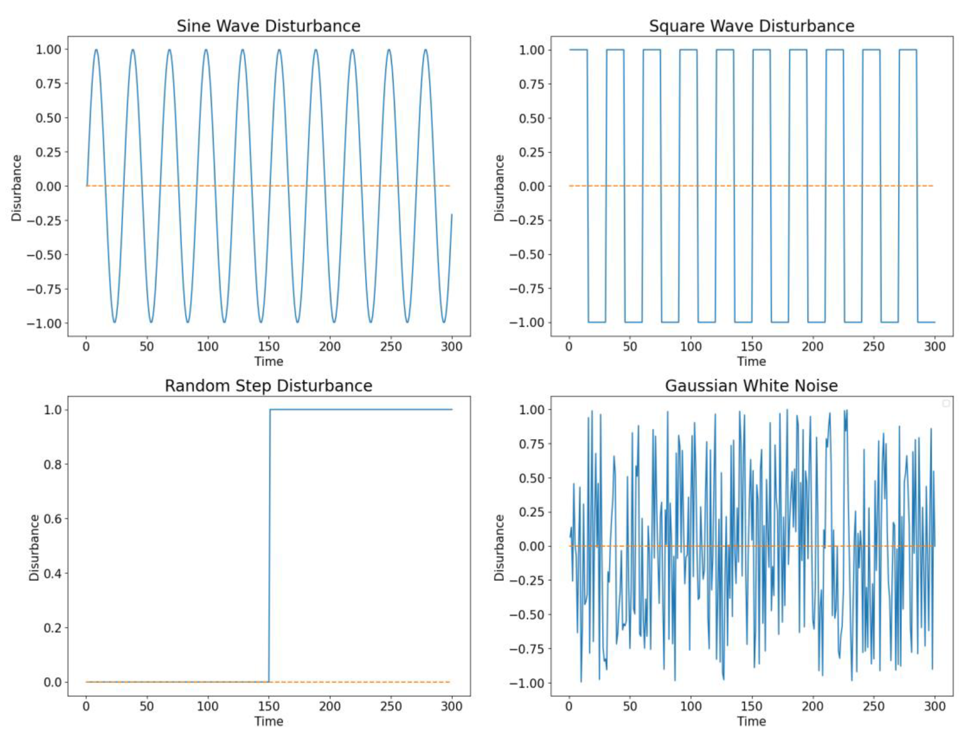
• Sine Wave Disturbance
  Sine wave disturbance is a common periodic disturbance used in simulations and engineering to mimic natural phenomena like wind, waves, or mechanical vibrations.
• Square Wave Disturbance
  Square wave disturbance simulates switching actions, motor step motions, or signal interference.
• Random Step Disturbance
  Random step disturbance simulates sudden changes like unexpected mechanical failures.
• Gaussian White Noise
  Gaussian white noise is statistical noise with equal power spectral density at all frequencies, represented by normally distributed random variables.

Modeling examples of the general interference types in the simulation scenario is shown in Figure 3.

4.2.2. Simulation Disturbance Types

1.

Dryden Turbulent Disturbance

The Dryden Turbulent Disturbance is based on the Dryden Turbulence Model, a fluid dynamics model used to describe turbulence phenomena in fluids. It primarily considers the turbulent viscosity effects of the fluid. The core idea of this model is to introduce an additional turbulent viscosity coefficient to correct the fluid’s viscosity. This model is widely used in engineering applications to simulate and analyze complex fluid flows, especially in fields involving turbulent flows, such as aerodynamics, hydraulics, and thermal engineering. Its mathematical model is as follows:

$$\begin{array}{c}n\left(t\right)=A+n_{shear}+n_{dryden}+n_{gust}\end{array}$$

(24)

where $n\left(t\right)$ is the total disturbance wind speed at time t, $A$ is the mean wind, $n_{shear}$ is the change in mean wind speed due to wind shear effects, $n_{dryden}$ is the turbulent random component on the total mean wind $\left(A+n_{shear}\right)$, and $n_{gust}$ is the wind speed due to gust effects.

2.

Random Natural Wind Disturbance

The random natural wind disturbance simulation model is a time series analysis model that combines the autocorrelation and random error effects in the data. It has constant mean, variance, and autocovariance, while also exhibiting characteristics of zero mean, constant variance, and mutual independence. Its general form is as follows:

$$\begin{array}{c}n\left(t\right)=c+{\displaystyle {\displaystyle \sum }_{i=1}^p}{\chi }_{1}n\left(t-\mathsf{\Delta }t\right)+{\displaystyle {\displaystyle \sum }_{i=1}^p}{\chi }_2{ϵ}_{t-\mathsf{\Delta }t}+{ϵ}_t\end{array}$$

(25)

In the equation, $n\left(t\right)$ is the wind speed at time $t$, $c$ is the constant term, ${\chi }_1$ and ${\chi }_2$ are parameters of the wind speed autocorrelation model and the disturbance correlation model, and ${ϵ}_t$ is the white noise sequence generated.

These environmental perturbations are of great significance for research in the field of drone control. By simulating different types of perturbations in simulations, reinforcement learning agents can learn control strategies that maintain good attitude stability in complex environments. This training not only improves the drone system’s ability to adapt to perturbations but also enhances the reinforcement learning algorithm itself, making it more effective in dealing with uncertainties and complex environments.

5. Setting Up a Simulation Environment

To validate the efficiency of algorithm training and the robustness of the model, we established a quadrotor simulation experimental environment. In this simulation, we emulated the effects of gravity and the aerodynamic model of a drone in real-world environments, while providing an interface for reinforcement learning. In this section, we will elaborate on some of the components involved in building this environment and the theoretical models of various simulation elements.

5.1. Development Components

5.1.1. OpenAI Gym

OpenAI Gym [27] is a toolkit that offers a diverse range of standardized environments for reinforcement learning algorithms, addressing various control and interaction problems. Each environment includes a unified set of interfaces, such as methods for initializing the environment, executing actions, receiving feedback, and visualizing the environment. Agents use this feedback to select actions and optimize their strategies. Additionally, OpenAI Gym provides sample environments and evaluation systems to assist developers in quickly starting, testing, and comparing algorithm performance.

In this study, we utilized its tools and libraries extensively for reinforcement learning training and model interaction. The standardized interfaces provided by it allowed us to seamlessly integrate our custom-built environment, facilitating the efficient execution of actions and the reception of feedback during training. This enabled us to test various reinforcement learning strategies and evaluate their performance in a controlled and consistent manner. The toolkit’s capabilities were crucial in setting up experiments, conducting rigorous testing, and performing thorough performance evaluations of the algorithms in our custom environment.

5.1.2. Bullet Physics

Bullet Physics [28] is an open-source physics engine designed for the accurate simulation of object motion and collisions. It supports efficient rigid and soft body dynamics, complex constraint handling systems, diverse collision detection algorithms, and interfaces for multiple programming languages. The engine utilizes optimized data structures and algorithms, such as BVH trees for rapid collision detection and solvers for stable dynamics simulations.

In this study, it provided the foundational simulation environment and dynamics suite essential for constructing our experimental scenarios. It was utilized for tasks including physical modeling in the simulation environment, ensuring the accurate representation of dynamic interactions, and enhancing the overall realism of the simulated tasks.

5.2. Quadrotor Model

5.2.1. The Mathematical Model of a Quadrotor

Building an accurate mathematical model is the foundation for understanding the dynamic behavior of quadrotors [29,30]. This section will delve into the dynamic model of a quadrotor, including specific descriptions of its position, velocity, and attitude angles, as well as rigid body motion and dynamic equations.

• Description of Position, Velocity, and Attitude

• Position Description:
  The position variables of the aircraft relative to the ground coordinate system are determined by $\left(\mathrm{x},\mathrm{y},\mathrm{z}\right)$, representing the lateral, longitudinal, and vertical positions of the aircraft in the ground coordinate system.
• Velocity Description:
  The velocity variables of the aircraft relative to the ground coordinate system are determined by $\left(\mathrm{u},\mathrm{v},\mathrm{w}\right)$, representing the lateral, longitudinal, and vertical velocities of the aircraft in the ground coordinate system.
• Attitude Description:
  The attitude of the aircraft is described by three angles $\left(\mathsf{\varphi },\mathsf{\theta },\mathsf{\psi }\right)$, where $\mathsf{\varphi }$ is the roll angle, $\mathsf{\theta }$ is the pitch angle, and $\mathsf{\psi }$ is the yaw angle.

These variables are the basis for precise control and stable flight, and they constitute the dynamic model of the aircraft.

2.

Assumptions

• Uniformly Symmetric Rigid Body Assumption:
  According to this assumption, all parts of the aircraft have the same density and mass distribution, ensuring symmetry and balance in the design and performance of the aircraft.
• Coincidence of Center of Mass and Geometric Center:
  The center of mass of the aircraft perfectly coincides with its geometric center, indicating that the weight of the aircraft is evenly distributed in space, which contributes to the stability and control accuracy of the aircraft.

3.

Rigid Body Motion and Dynamic Equations

The motion of a rigid body consists of the translation of its center of mass and the rotation about its center of mass, which is the conclusion of Newton–Euler equations. For a quadrotor aircraft, we can represent its dynamics using the following equations:

• Translation Equations (Differential Equations of Position and Velocity):
  This equation reflects how the position and velocity of the aircraft change, helping us understand the translational motion of the aircraft.

  $$\begin{array}{c}\left\{\begin{array}{c}\ddot{x}=-\frac{f}{m}\left(\cos \psi \sin \theta \cos \varphi +\sin \psi \sin \varphi \right)\\ \ddot{y}=-\frac{f}{m}\left(\sin \psi \sin \theta \cos \varphi -\cos \psi \sin \varphi \right)\\ \ddot{z}=g-\frac{f}{m}\cos \varphi \cos \theta \end{array}\right.\#\end{array}$$

  (26)
• Rotation Equations (Differential Equations of Attitude Angles):
  This equation describes the changes in the aircraft’s attitude angles, which are used to represent the rotational motion of the aircraft.

  $$\begin{array}{c}\left\{\begin{array}{c}\ddot{\varphi }=\frac{1}{I_x}\left[l{f}_{\varphi }+\dot{\theta }\dot{\psi }\left(I_y-I_z\right)\right]\\ \ddot{\theta }=\frac{1}{I_y}\left[l{f}_{\theta }+\dot{\varphi }\dot{\psi }\left(I_z-I_x\right)\right]\\ \ddot{\psi }=\frac{1}{I_z}\left[l{f}_{\psi }+\dot{\theta }\dot{\varphi }\left(I_x-I_y\right)\right]\end{array}\right.\end{array}$$

  (27)

  where $f_{\varphi },f_{\theta }, and f_{\psi }$ represent the torques generated by the rotors on the three axes due to the lift force; $I_x,I_y,and I_z$ are the moments of inertia of the rotors and motors rotating around the $x$-axis, $y$-axis, and $z$-axis respectively; $l$ is the distance between the center of mass of the aircraft’s body and its rotor rotation axis.

These equations can express and predict the dynamic performance of the quadrotor, such as changes in its position, velocity, and attitude. These models provide theoretical foundations for control strategy design and simulation analysis. These equations use Newton–Euler equations, incorporating the aircraft’s mass, torques, and moments of inertia, which are essential for the flight control and hover control of the aircraft.

5.2.2. Aerodynamic Effects

To accurately analyze the flight characteristics and stability of a quadrotor aircraft, it is essential to consider the impact of aerodynamic effects during the modeling and control of the quadrotor. This section will elaborate on the major aerodynamic effects encountered by a quadrotor during flight, including the lift effect and ground effect.

• Lift Effect

The lift effect, denoted as $D$, is crucial for the quadrotor aircraft to achieve vertical take-off and landing as well as hovering. It is represented by the lift force generated by the propellers and is proportional to the velocity $v$ of the aircraft. The formula for calculating lift is as follows:

$$\begin{array}{c}D=-k_D\left({\displaystyle {\displaystyle \sum }_{i=1}^4}2\pi P_i\right)v\end{array}$$

(28)

where $k_D$ is a lift coefficient, $P_i$ is the rotational speed of the $i$-th propeller, and $x$ is the linear velocity of the quadrotor.

In practical applications, the lift effect is the primary control factor for the vertical take-off and landing, hovering, and flight altitude control of the aircraft. This effect plays a central role in the design and control system of drones.

2.

Ground Effect

Ground effect refers to the phenomenon of increased thrust when the aircraft approaches the ground. This effect is proportional to the propeller radius $r_{P_i}$, the rotational speed of the motor $P_i$, the height $h_i$ of the quadrotor from the ground, and the ground effect coefficient $G_L$. The formula for calculating ground effect is as follows:

$$\begin{array}{c}G=G_L{\displaystyle {\displaystyle \sum }_{i=1}^4}{\left(\frac{r_{P_i}}{h_i}\right)}^2{P}_i^2\end{array}$$

(29)

where $G_L$ is the ground effect coefficient, which increases as the ground is approached, and $G$ represents the additional thrust of each motor due to the ground effect. Ground effect is particularly important during the take-off and landing phases of the aircraft, as it can provide additional lift and reduce energy consumption.

6. Experimental Analysis

On the quadrotor simulation experimental platform, we conducted a series of experiments to validate the effectiveness of the Multi-PID Self-Attention guiding module. Through the flight controller trained by reinforcement learning, we conducted detailed evaluations and analyses of the flight performance under different scenarios and compared the improved DRL algorithm using the Multi-PID Self-Attention guiding module with the original DRL algorithm.

6.1. Experimental Verification of the Module to Eliminate PID Parameter Sensitivity

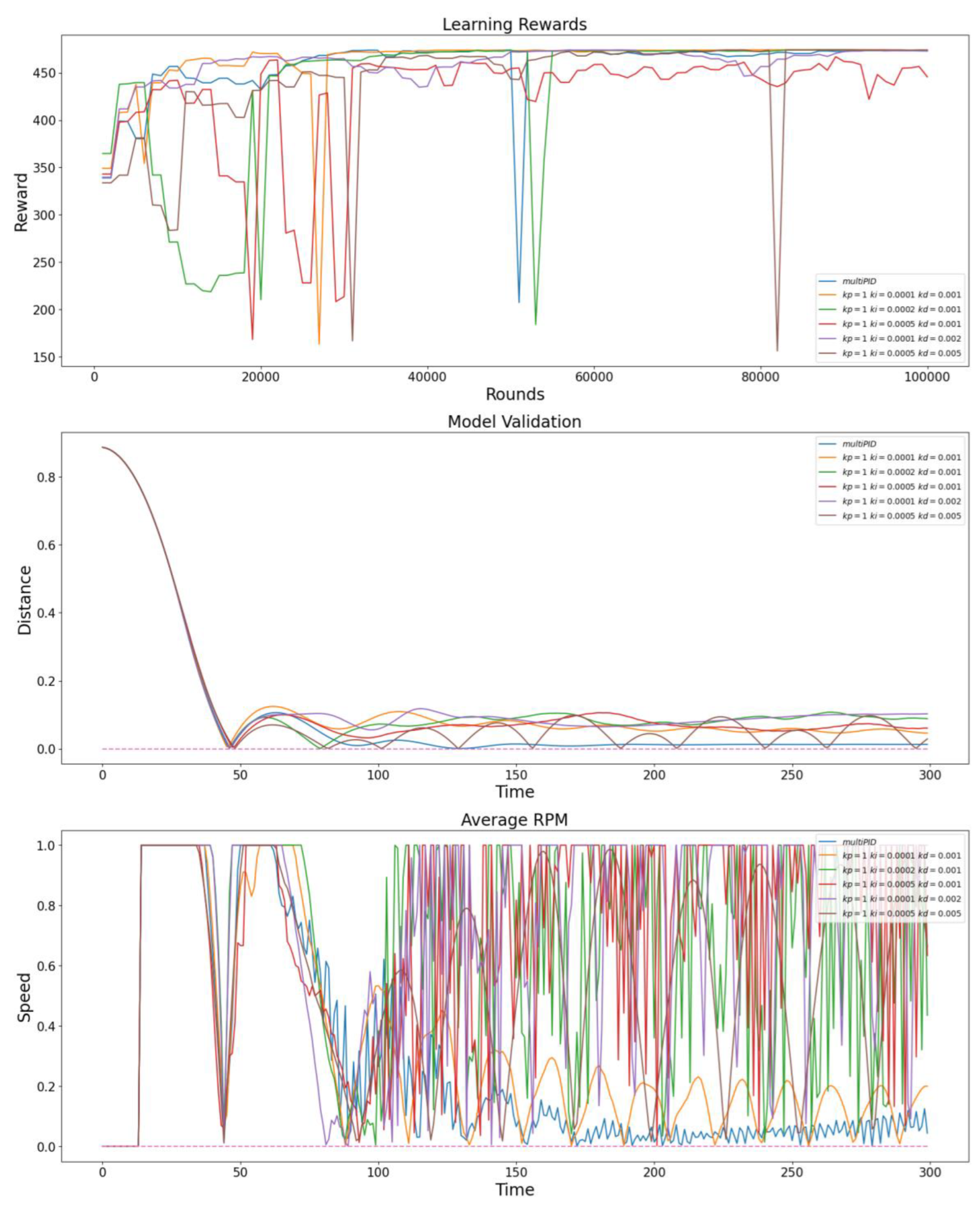
In this section, we conducted training guidance for the original PPO algorithm under feedback from multiple PID controllers with different parameters and compared it with the PPO algorithm improved by the Multi-PID Self-Attention guiding module. This guiding module consists of five PID controllers, with parameters of the same order of magnitude as a single PID controller. As shown in Figure 4, we compared the variation trends in model rewards during training, the displacement changes in the model from entity to target position in the simulation environment after training, and the average rotor speed of the entity.

From the analysis of the data in Figure 4, under the condition that the parameters are within the same order of magnitude, the algorithm optimized with the Multi-PID Self-Attention guiding module exhibits greater stability during training. The model generated by this algorithm can achieve more stable hovering near the target point and better control of rotor speed after reaching the steady state, demonstrating improved training effectiveness. The experimental results further validate that the dynamic attention allocation mechanism of the Multi-PID Self-Attention guiding module effectively reduces the determinative impact of a single PID controller on the model’s global behavior, preventing excessive decision fluctuations near the zero point of a single PID controller.

6.2. Comparison of Training Stability under Different Learning Rates

In this section, we use the PPO algorithm as the baseline DRL framework and compare the experimental results under different learning rate settings. We explore in detail the training efficiency and model performance of the DRL algorithm before and after optimization with the Multi-PID Self-Attention guiding module. This aims to objectively evaluate the practical effectiveness and impact of the Multi-PID Self-Attention guiding module during the training process.

6.2.1. Training Efficiency of the Algorithm under Different Learning Rate Settings

In this section, we discuss the performance of the PPO algorithm optimized by the Multi-PID Self-Attention guidance module and the original PPO algorithm during the training process under different learning rate settings.

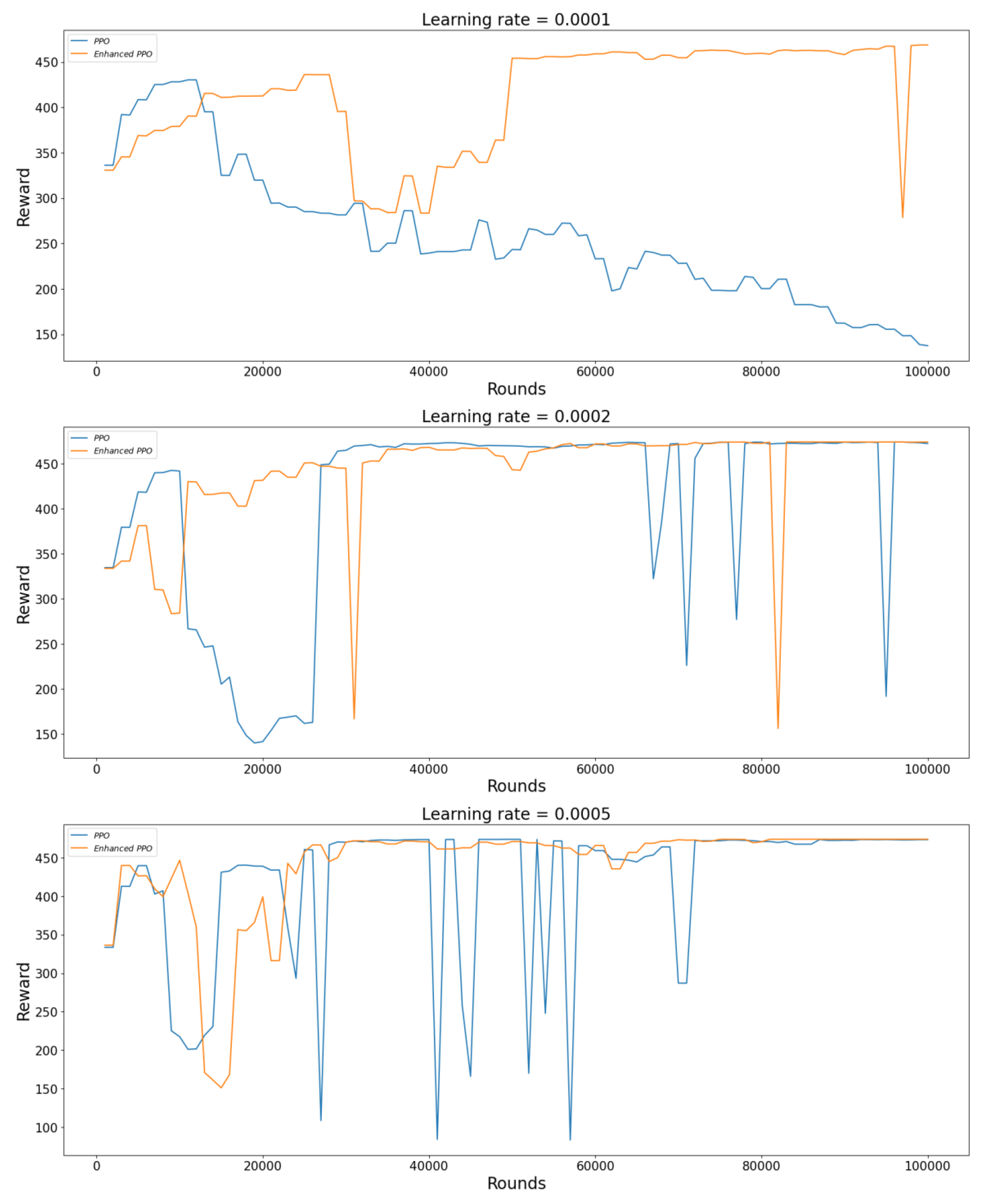
As can be seen from Figure 5, the algorithm optimized by the Multi-PID Self-Attention guidance module, compared to before the optimization, can better maintain a high level of training reward without allowing it to decline for a prolonged period, indicating that the improved algorithm is more stable during training. Furthermore, while the improved reward function in this study is generally slightly lower than before the improvement, during the experimental process, the upper limit of state rewards explored by both the improved and original algorithms is almost similar, suggesting that the actual training effect of the model is superior.

6.2.2. Model Performance under Different Learning Rate Settings

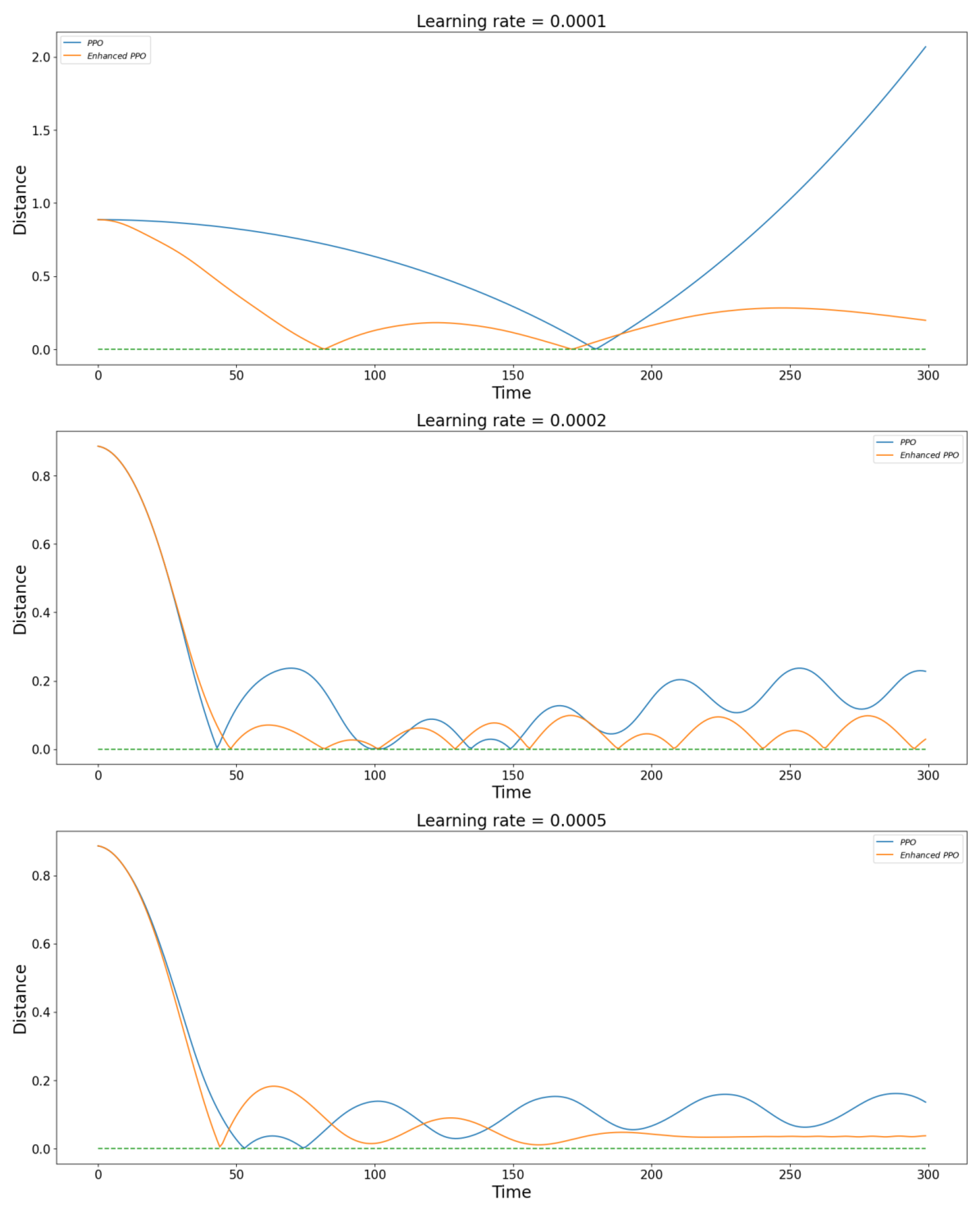
In this section, we will observe the actual performance of the PPO algorithm model in the simulation environment after the same training period, both before and after optimization with the Multi-PID Self-Attention guiding module, under different learning rate settings.

Figure 6 shows the performance of the PPO algorithm optimized by the Multi-PID Self-Attention guidance module and the original PPO algorithm after 100,000 training iterations under different learning rates. From Figure 6, we can observe that the improved algorithm model achieves better control effects for each learning rate setting. When the learning rate is 0.0001, while the original model can only reach the target position once in 300 simulation cycles, the improved model can reach the target twice in the same simulation cycle and has a more apparent trend of convergence. At a learning rate of 0.0002, both the original and improved models achieve jittering around the target point, but the jittering center of the original model gradually deviates from the target point, and its average distance from the target point is significantly further. At a learning rate of 0.0005, the original model does not achieve significant improvement, as it still jitters away from the target point, while the improved model successfully eliminates the jitter after a brief adjustment, achieving a normal hovering state.

6.3. Verification of Algorithm Robustness under Different Disturbance Environments

In this section, we conducted simulation experiments under various disturbed environments, including sine wave, square wave, random step, and Gaussian white noise. We also performed ablation experiments on four algorithms, the improved PPO algorithm, the improved PPO algorithm without the self-attention module, the improved PPO algorithm trained only in undisturbed environments, and the original PPO algorithm, to evaluate the practical effectiveness of the deep reinforcement learning framework designed in this study.

6.3.1. Training Efficiency of Algorithms under Different Disturbed Environments

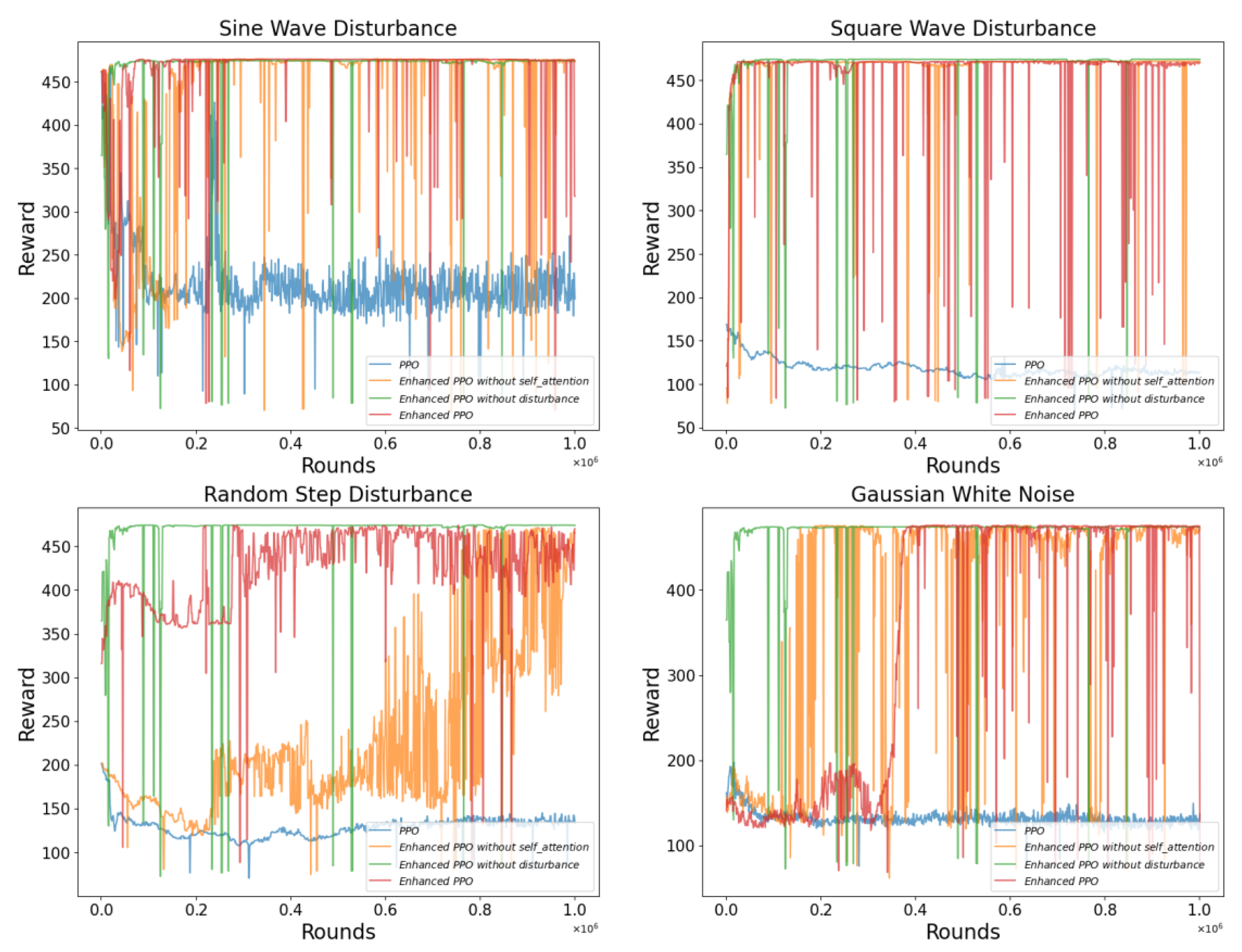
In this section, we conducted simulation experiments under various disturbance environments, including sinusoidal waves, square waves, random step disturbances, and Gaussian white noise. We performed ablation experiments on three DRL algorithms—A2C, SAC, and PPO. The ablation targets included the improved DRL algorithm, the improved DRL algorithm without the self-attention module, the improved DRL algorithm trained only in a non-disturbance environment, and the original DRL algorithm. This was carried out to evaluate the effectiveness of the DRL framework designed in this study in enhancing model training.

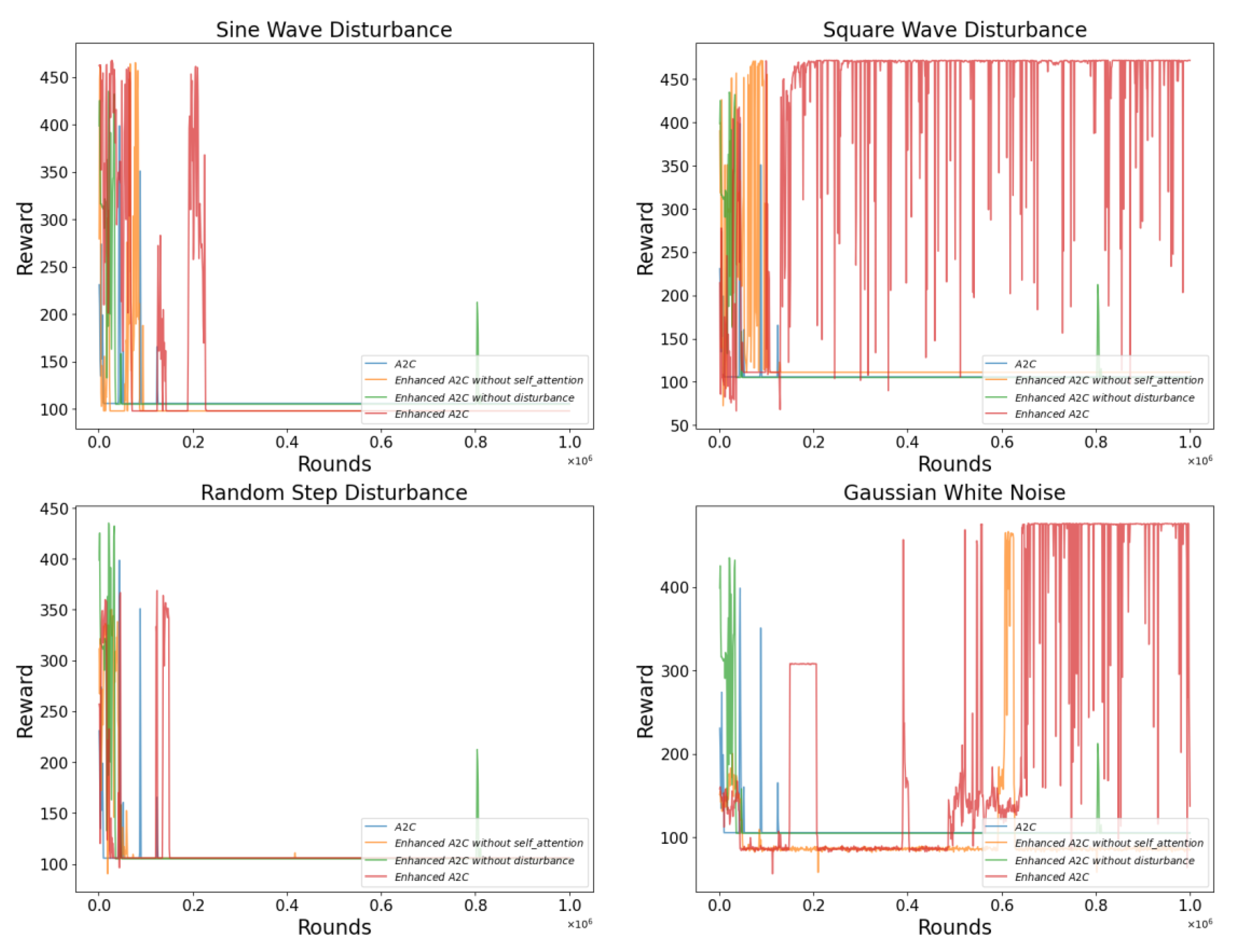
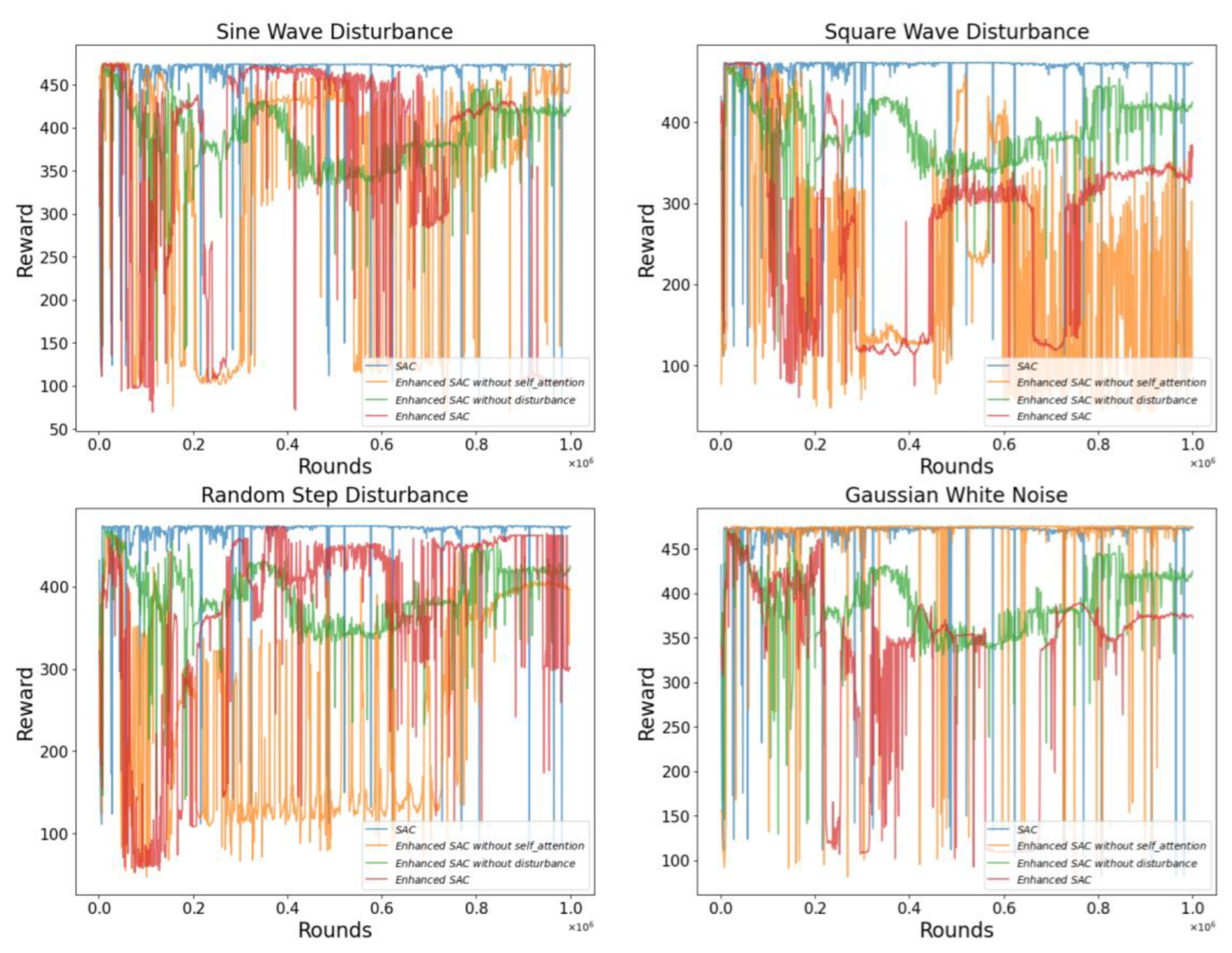
From Figure 7, Figure 8 and Figure 9, it is evident that the original A2C and PPO algorithms struggle to achieve effective training in disturbed environments. As shown in Figure 7, the A2C algorithm optimized with the self-attention module exhibits some improvement in state exploration under sinusoidal wave and random step disturbances. However, in sinusoidal wave and Gaussian white noise disturbances, the enhanced A2C algorithm significantly outperforms other targets in the ablation experiments. Figure 8 indicates that the optimized SAC algorithm does not show a clear advantage in the four disturbance environments. Only under random step disturbances does the self-attention module demonstrate a good guiding effect on training. As depicted in Figure 9, under random step and Gaussian white noise disturbances, the improved PPO algorithm without the Multi-PID Self-Attention guiding module performs poorly during training, failing to reach the performance level of the enhanced PPO algorithm.

6.3.2. Model Performance under Different Disturbed Environments

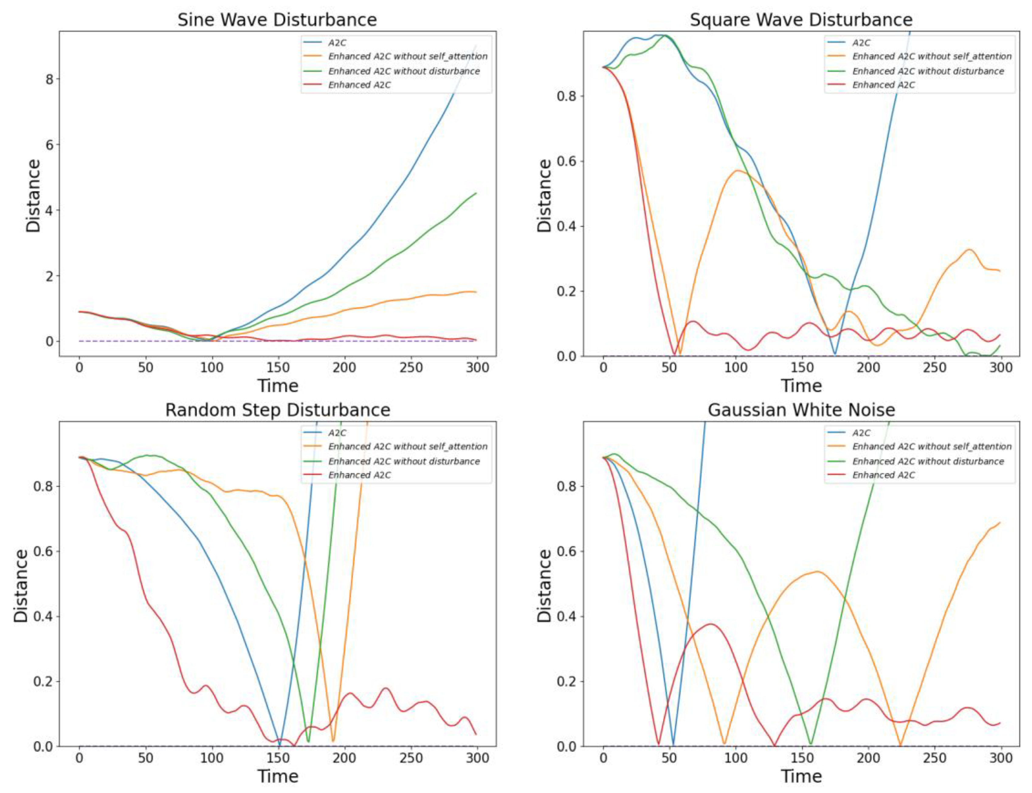
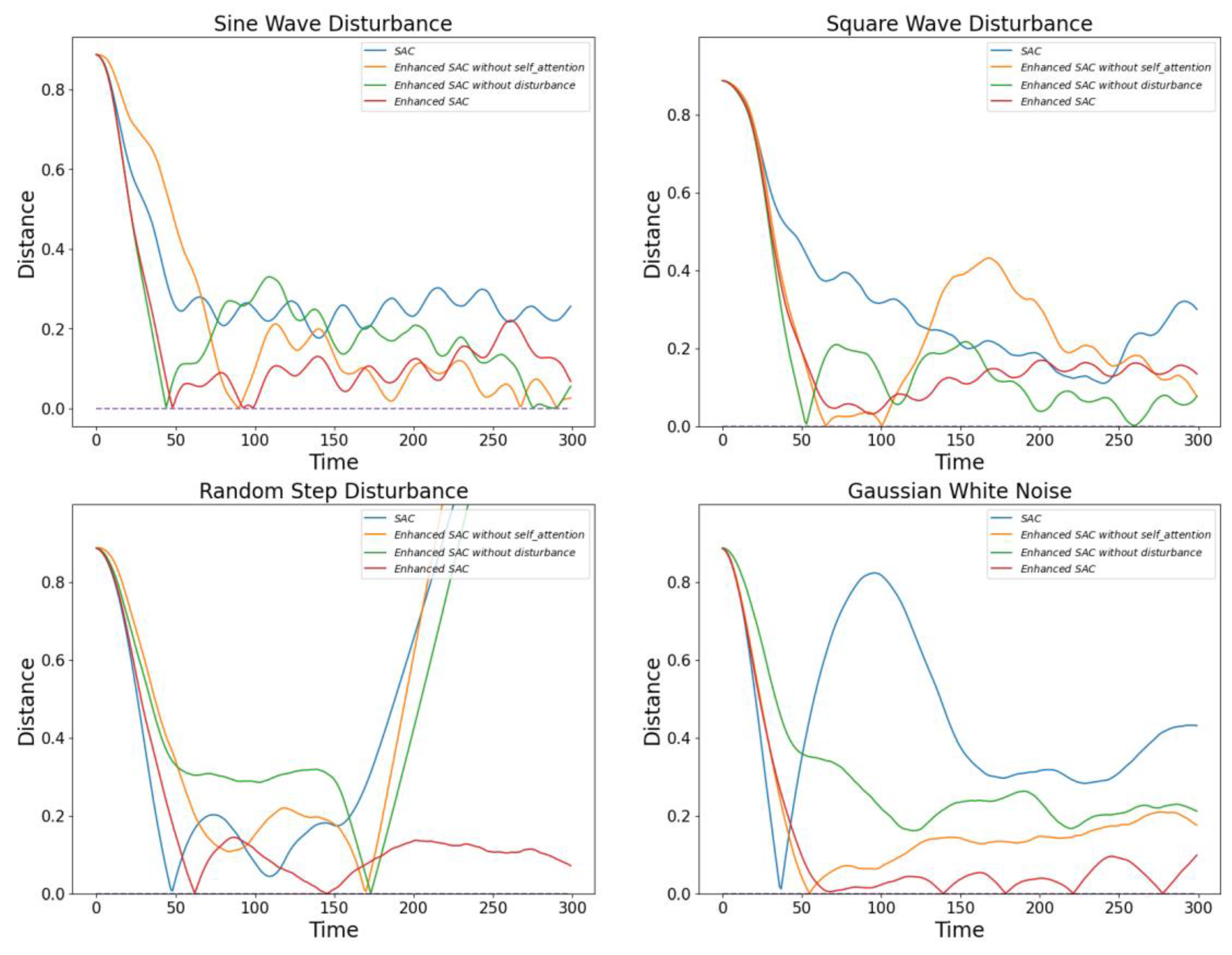
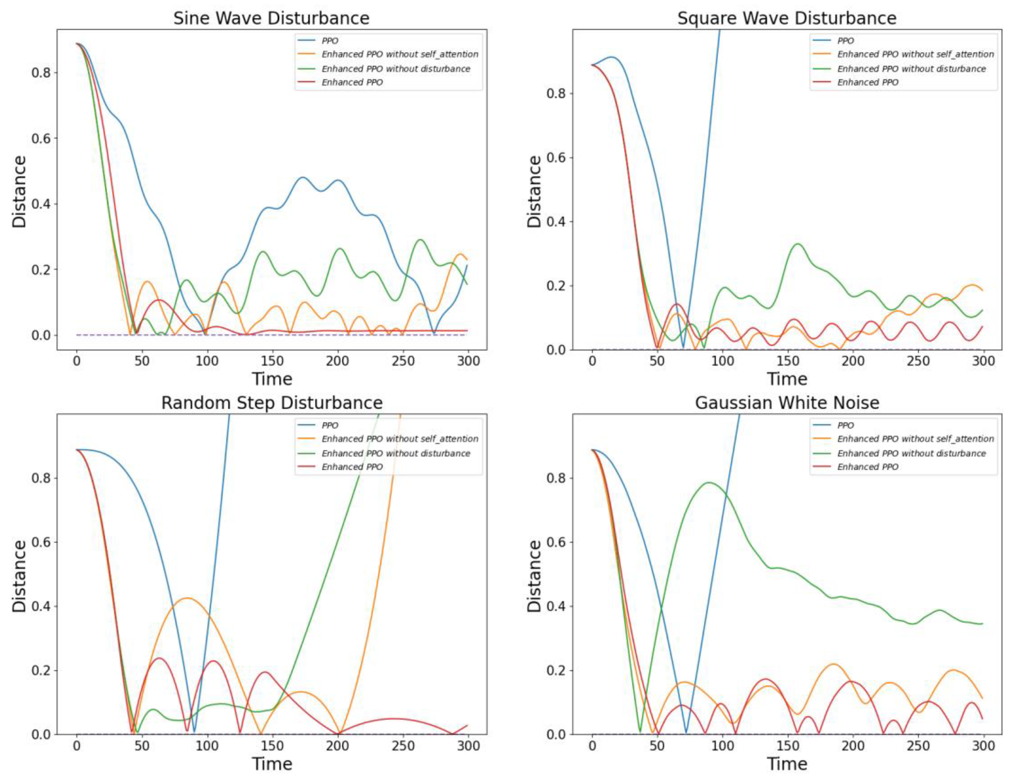
In this section, we conducted ablation experiments to evaluate the final training effectiveness of the models under the same disturbance environments, including sinusoidal waves, square waves, random step disturbances, and Gaussian white noise. We performed ablation experiments on three DRL algorithms. Although guiding the model to achieve higher reward values during training is important, the ultimate focus of our experiments is on the final training effectiveness of the models. This approach ensures that the evaluation centers on the practical performance improvements of the trained models.

Figure 10, Figure 11 and Figure 12 show the performance of the three algorithms after 1 million training iterations under different disturbance environments.

Figure 10 illustrates the performance of the optimized A2C model in four different disturbance environments. It can be observed that the optimized A2C model shows significant performance improvement in each type of disturbance setting. This indicates that the optimization measures effectively enhance the adaptability and stability of the A2C model in variable environments.

Further, Figure 11 describes the performance of the SAC model under the four disturbance environments. Although the optimization effects of the SAC model are not particularly significant in the sinusoidal wave and square wave disturbance environments, the model demonstrates notable advantages in the other two disturbance environments. This finding reveals potential performance differences in the SAC model under various types of disturbances.

Regarding the PPO algorithm shown in Figure 12, the improved PPO algorithm exhibits excellent adaptability and stability across all disturbance environments. Particularly when dealing with random step disturbances, the improved PPO algorithm can quickly adjust its strategy to maintain superior attitude stability. In contrast, the original PPO algorithm and the improved PPO algorithm without the multi-head self-attention module perform poorly during training. Although the original PPO algorithm can quickly achieve high reward states in a disturbance-free environment, it shows poor robustness in disturbed environments. These observations further confirm the importance of optimizing algorithm models for different disturbance environments.

6.3.3. Model Performance under Different Disturbed Environments

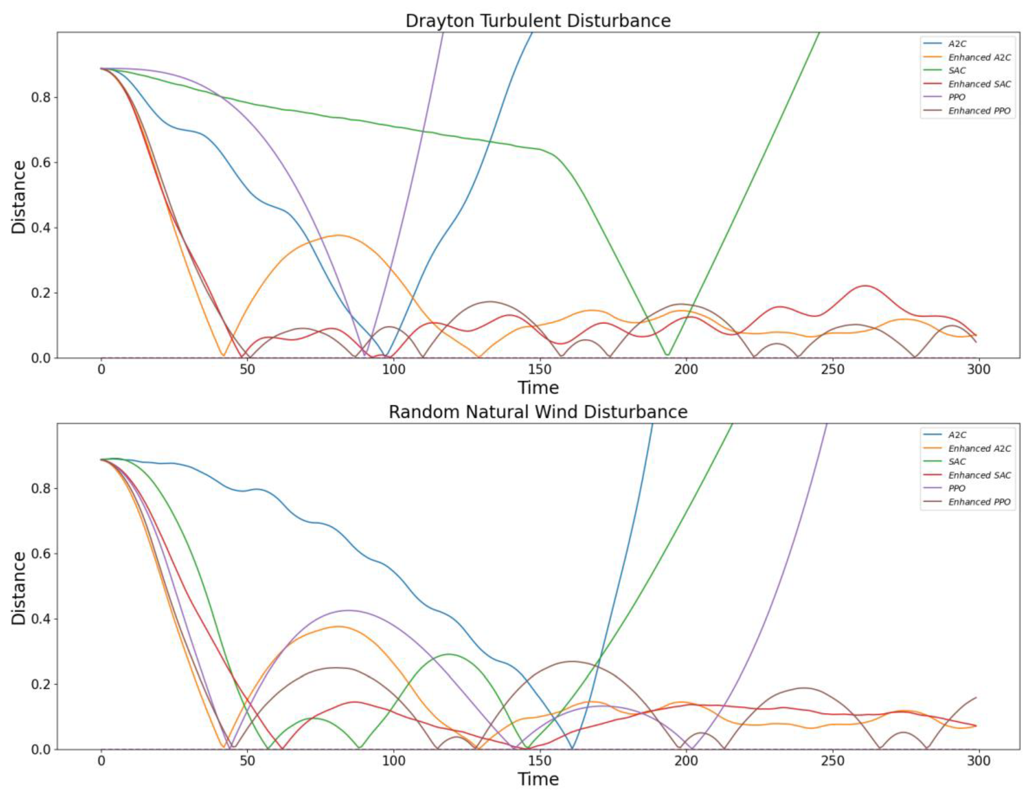
In this section, we evaluate the enhancement effects of three deep reinforcement learning (DRL) algorithms under Dryden turbulence and random natural wind disturbances. The algorithms assessed include A2C, SAC, and PPO-Clip. Each algorithm’s performance is measured in terms of stability in a simulated flight environment, considering the disturbances mentioned.

As shown in Figure 13, the comparative analysis indicates that while all three algorithms benefit from the introduction of advanced control mechanisms, PPO-Clip outperforms A2C and SAC in terms of robustness and stability under Dryden turbulence and random natural wind disturbances. The results highlight the importance of incorporating entropy-based exploration and reliable policy updates in enhancing the performance of DRL algorithms in complex and dynamic environments.

7. Conclusions

This study proposes a novel module that integrates the PID control strategy with the state reward function. Utilizing a self-attention mechanism, it optimizes action output in a drone simulation environment, thereby enhancing the training efficiency of deep reinforcement learning. The experimental results indicate that the DRL algorithm employing the Multi-PID Self-Attention guiding module achieves significant improvements in training stability and efficiency. This algorithm uses the PID control strategy to effectively reduce policy parameter fluctuations, prevent drastic policy changes, and enhance the stability of the training process. Moreover, the optimized DRL algorithm converges more quickly, significantly shortening the training cycle.

Additionally, the optimized DRL algorithm demonstrates greater robustness to various environmental disturbances. In the experiments, we set up environments with sinusoidal wave disturbances, square wave disturbances, random step disturbances, and Gaussian white noise. The results show that the optimized DRL algorithm exhibits superior adaptability and stability in these disturbed environments. Particularly when facing random step disturbances, the optimized DRL algorithm quickly adjusts the strategy and maintains good attitude stability, while the original DRL algorithm and the version without the self-attention module perform less effectively.

Our current research findings have been applied to various simulated task scenarios involving drones, including obstacle avoidance, path following, and complex maneuver execution, thereby aiding the execution of navigation planning tasks by drone entities. There are still many aspects worth exploring further in the results of this study. On the one hand, the improved DRL algorithm can be applied to other drone control tasks, such as hexacopter drones and fixed-wing drones, to test its universality and applicability. On the other hand, attempts can be made to combine the Multi-PID Self-Attention guiding module with other advanced control strategies, such as fuzzy control and sliding mode control, to enhance the control performance of drones. Additionally, applying the Multi-PID Self-Attention guiding module on real drone systems to validate its effectiveness and reliability in practical operating environments is also an important direction for future research.

References

- Martiskainen, M.; Coburn, J. The role of information and communication technologies (ICTs) in household energy consumption-prospects for the UK. Energy Effic. 2011, 4, 209–221. [Google Scholar] [CrossRef]
- Mohsan, S.A.H.; Khan, M.A.; Noor, F.; Ullah, I.; Alsharif, M.H. Towards the unmanned aerial vehicles (UAVs): A comprehensive review. Drones 2022, 6, 147. [Google Scholar] [CrossRef]
- Liu, R.; Nageotte, F.; Zanne, P.; de Mathelin, M.; Dresp-Langley, B. Deep reinforcement learning for the control of robotic manipulation: A focussed mini-review. Robotics 2021, 10, 22. [Google Scholar] [CrossRef]
- Khalil, M.; McGough, A.S.; Pourmirza, Z.; Pazhoohesh, M.; Walker, S. Machine Learning, Deep Learning and Statistical Analysis for forecasting building energy consumption—A systematic review. Eng. Appl. Artif. Intell. 2022, 115, 105287. [Google Scholar] [CrossRef]
- Willis, M.J. Proportional-Integral-Derivative Control; Department of Chemical and Process Engineering, University of Newcastle: Callaghan, Australia, 1999; Volume 6. [Google Scholar]
- Kwon, Y.; Kim, C.; Peisert, S.; Bishop, M.; Yoon, I. A2c: Self Destructing Exploit Executions via Input Perturbation. In Proceedings of the Network and Distributed System Security Symposium, San Diego, CA, USA, 26 February–1 March 2017. [Google Scholar]
- Haarnoja, T.; Zhou, A.; Abbeel, P.; Levine, S. Soft actor-critic: Off-policy maximum entropy deep reinforcement learning with a stochastic actor. In Proceedings of the International Conference on Machine Learning, Stockholm, Sweden, 10–15 July 2018; pp. 1861–1870. [Google Scholar]
- Schulman, J.; Wolski, F.; Dhariwal, P.; Radford, A.; Klimov, O. Proximal policy optimization algorithms. arXiv 2017, arXiv:1707.06347. [Google Scholar]
- Zhao, W.; Queralta, J.P.; Westerlund, T. Sim-to-real transfer in deep reinforcement learning for robotics: A survey. In Proceedings of the 2020 IEEE Symposium Series on Computational Intelligence (SSCI), Canberra, ACT, Australia, 1–4 December 2020; pp. 737–744. [Google Scholar]
- Kang, K.; Belkhale, S.; Kahn, G.; Abbeel, P.; Levine, S. Generalization through simulation: Integrating simulated and real data into deep reinforcement learning for vision-based autonomous flight. In Proceedings of the 2019 International Conference on Robotics and Automation (ICRA), Montreal, QC, Canada, 20–24 May 2019; pp. 6008–6014. [Google Scholar]
- Mahmud, S.K.; Liu, Y.; Chen, Y.; Chai, K.K. Adaptive reinforcement learning framework for NOMA-UAV networks. IEEE Commun. Lett. 2021, 25, 2943–2947. [Google Scholar] [CrossRef]
- Bekar, C.; Yuksek, B.; Inalhan, G. High fidelity progressive reinforcement learning for agile maneuvering UAVs. In Proceedings of the AIAA Scitech 2020 Forum, Orlando, FL, USA, 6–10 January 2020; p. 0898. [Google Scholar]
- Koch, W.; Mancuso, R.; West, R.; Bestavros, A. Reinforcement learning for UAV attitude control. ACM Trans. Cyber-Phys. Syst. 2019, 3, 1–21. [Google Scholar] [CrossRef]
- Guo, T.; Jiang, N.; Li, B.; Zhu, X.; Wang, Y.; Du, B. UAV navigation in high dynamic environments: A deep reinforcement learning approach. Chin. J. Aeronaut. 2021, 34, 479–489. [Google Scholar] [CrossRef]
- Cavanini, L.; Ippoliti, G.; Camacho, E.F. Model predictive control for a linear parameter varying model of an UAV. J. Intell. Robot. Syst. 2021, 101, 57. [Google Scholar] [CrossRef]
- Siti, I.; Mjahed, M.; Ayad, H.; El Kari, A. New trajectory tracking approach for a quadcopter using genetic algorithm and reference model methods. Appl. Sci. 2019, 9, 1780. [Google Scholar] [CrossRef]
- Kurnaz, S.; Cetin, O.; Kaynak, O. Fuzzy logic based approach to design of flight control and navigation tasks for autonomous unmanned aerial vehicles. J. Intell. Robot. Syst. 2009, 54, 229–244. [Google Scholar] [CrossRef]
- Din, A.F.U.; Mir, I.; Gul, F.; Al Nasar, M.R.; Abualigah, L. Reinforced learning-based robust control design for unmanned aerial vehicle. Arab. J. Sci. Eng. 2023, 48, 1221–1236. [Google Scholar] [CrossRef]
- Fang, Y.; Yao, Y.; Zhu, F.; Chen, K. Piecewise-potential-field-based path planning method for fixed-wing UAV formation. Sci. Rep. 2023, 13, 2234. [Google Scholar] [CrossRef] [PubMed]
- Meng, Q.; Chen, K.; Qu, Q. PPSwarm: Multi-UAV Path Planning Based on Hybrid PSO in Complex Scenarios. Drones 2024, 8, 192. [Google Scholar] [CrossRef]
- Ou, L.; Yao, Y.; Luo, X.; Li, X.; Chen, K. ContextAD: Context-Aware Acronym Disambiguation with Siamese BERT Network. Int. J. Intell. Syst. 2023, 2023, 5014355. [Google Scholar] [CrossRef]
- Wang, C.; Wang, J.; Shen, Y.; Zhang, X. Autonomous navigation of UAVs in large-scale complex environments: A deep reinforcement learning approach. IEEE Trans. Veh. Technol. 2019, 68, 2124–2136. [Google Scholar] [CrossRef]
- Bayerlein, H.; De Kerret, P.; Gesbert, D. Trajectory optimization for autonomous flying base station via reinforcement learning. In Proceedings of the 2018 IEEE 19th International Workshop on Signal Processing Advances in Wireless Communications (SPAWC), Kalamata, Greece, 25–28 June 2018; pp. 1–5. [Google Scholar]
- Rodriguez-Ramos, A.; Sampedro, C.; Bavle, H.; De La Puente, P.; Campoy, P. A deep reinforcement learning strategy for UAV autonomous landing on a moving platform. J. Intell. Robot. Syst. 2019, 93, 351–366. [Google Scholar] [CrossRef]
- Wang, Y.; Zhan, S.S.; Jiao, R.; Wang, Z.; Jin, W.; Yang, Z.; Wang, Z.; Huang, C.; Zhu, Q. Enforcing hard constraints with soft barriers: Safe reinforcement learning in unknown stochastic environments. In Proceedings of the International Conference on Machine Learning, Honolulu, HI, USA, 23–29 July 2023; pp. 36593–36604. [Google Scholar]
- Zhang, D.; Tang, Y.; Zhang, W.; Wu, X. Hierarchical design for position-based formation control of rotorcraft-like aerial vehicles. IEEE Trans. Control Netw. Syst. 2020, 7, 1789–1800. [Google Scholar] [CrossRef]
- Brockman, G.; Cheung, V.; Pettersson, L.; Schneider, J.; Schulman, J.; Tang, J.; Zaremba, W. Openai gym. arXiv 2016, arXiv:1606.01540. [Google Scholar]
- Coumans, E. Bullet physics simulation. In Proceedings of the ACM SIGGRAPH 2015 Courses, Los Angeles, CA, USA, 9–13 August 2015; p. 1. [Google Scholar]
- Dong, W.; Gu, G.Y.; Zhu, X.; Ding, H. Modeling and control of a quadrotor UAV with aerodynamic concepts. World Acad. Sci. Eng. Technol. 2013, 7, 901–906. [Google Scholar]
- Yoo, D.W.; Oh, H.D.; Won, D.Y.; Tahk, M.J. Dynamic modeling and control system design for Tri-Rotor UAV. In Proceedings of the 2010 3rd International Symposium on Systems and Control in Aeronautics and Astronautics, Harbin, China, 8–10 June 2010; pp. 762–767. [Google Scholar]