Multi-UAV Cooperative Localization Using Adaptive Wasserstein Filter with Distance-Constrained Bare Bones Self-Recovery Particles

Abstract

Aiming at the cooperative localization problem for the dynamic UAV swarm in an anchor-limited environment, an adaptive Wasserstein filter (AWF) with distance-constrained bare bones self-recovery particles (CBBP) is proposed. Firstly, to suppress the cumulative error from the inertial navigation system (INS), a position-prediction strategy based on transition particles is designed instead of using inertial measurements directly, which ensures that the generated prior particles can better cover the ground truth and provide the uncertainties of nonlinear estimation. Then, to effectively quantify the difference between the observed and the prior data, the Wasserstein measure based on slice segmentation is introduced to update the posterior weights of the particles, which makes the proposed algorithm robust against distance-measurement noise variance under the strongly nonlinear model. In addition, to solve the problem of particle impoverishment caused by traditional resampling, a diversity threshold based on Gini purity is designed, and a fast bare bones particle self-recovery algorithm with distance constraint is proposed to guide the outlier particles to the high-likelihood region, which effectively improves the accuracy and stability of the estimation. Finally, the simulation results show that the proposed algorithm is robust against cumulative error in an anchor-limited environment and achieves more competitive accuracy with fewer particles.

1. Introduction

Multiple unmanned aerial vehicle (UAV) systems have a wide range of applications, including patrol inspection [1], urban rescue [2,3], and military surveillance [4,5,6]. In most scenarios, using global navigation satellite systems (GNSSs) to obtain an accurate position is the key to successfully completing various applications. However, in harsh environments, such as forests and urban canyons, reliable GNSS positioning cannot be ensured, generally [7]. Using relative measurement information from nodes with precise positioning information, cooperative localization [8,9,10] is a solution to obtaining accurate positions in GPS-denied locations.

There is a significant amount of research on the cooperative localization problem. One strategy is based on non-Bayesian estimation [11,12,13]. It treats the location information of UAVs as unknown deterministic parameters, which reduces localization accuracy. For example, time-of-arrival cooperative localization (TOA-CL) [11] roughly linearizes a nonlinear measurement function so that there is room for improvement in estimation accuracy. The maximum likelihood and iterative localization algorithm (ML-ILA) [12] integrates GNSS and relative distance information, following the ML strategy to solve a quadratic non-convex programming problem. Although positioning accuracy has been dramatically improved, it does not consider communication costs and only considers static scenarios, and the algorithm’s scalability needs further research. The vBFGs algorithm [13] considers the velocity and distance information of UAVs and transforms the cooperative localization problem into an optimization problem solved by the BFGs algorithm. Although it retains the nonlinearity of the model, the global convergence of the algorithm in particular scenarios needs further optimization.

Another important strategy is based on Bayesian estimation [14,15,16,17,18]. This method [19] fully utilizes the prior information of nodes for unknown estimation and is expected to be a better estimation method. To mention a few examples, an adaptive extended Kalman filter (A-EKF) achieves high localization accuracy by estimating the prediction error covariance matrix and measurement noise covariance matrix [14]. However, its computational complexity is high, making it challenging to meet the response requirements of a UAV swarm. Global state-covariance intersection (GS-CI) [15] provides a bound criterion for the covariance matrix of intelligent UAVs and maintains estimation consistency by using the intersection of covariances in communication updates. However, it can only be used in static networks, and its adaptability to dynamic networks needs further exploration. The DEKF algorithm [16] analyzes the causes of time delay in the process of robot cooperative localization, and then introduces the communication time delay into the state and measurement equations, reconstructs the state equation and measurement equation of the robot, and improves the performance of the extended Kalman filter algorithm. However, the algorithm is sensitive to abnormal data loss and lacks robustness in harsh environments. In addition, the $H\infty$ filter [17] is an estimation method whose design parameters are sensitive in harsh outdoor environments.

It should be noted that the above filter-based method cannot handle nonlinear problems. However, in a multi-UAV system, the nonlinearity of the dynamic and observation model makes the cooperative localization problem have high nonlinearity. To solve this problem, some researchers employ sampling methods to approximate the nonlinear distribution to solve nonlinear problems. The most representative ones include the particle filter (PF) algorithm and the unscented Kalman filter (UEKF) algorithm. All of them are based on the Bayesian filtering framework and estimate the system state recursively through two steps of prediction and update. UEKF is suitable for Gaussian distribution and moderately nonlinear cases by combining the linearization method of EKF with unscented transformation. In addition, if the condition number of the system model or the noise covariance matrix is poor, using UKF may lead to unstable calculations or inaccurate localization results [20].

As a sequential Monte Carlo method, particle filtering is a feasible solution to this problem [21]. It can be applied to any dynamic state-space model. Based on the traditional particle filter algorithm, some research methods have been proposed to enhance the positioning accuracy [22,23]. For example, to solve the problem that the traditional algorithm can not effectively reflect the effectiveness of the observation information, due to the average weighting of the particles, the optimal weighted-particle filter (OWPF) [22] uses the observation variance as the weight, which effectively improves the positioning accuracy. The particle filter-based indoor navigation (PFIN) algorithm [23] uses an optimized localization algorithm (OLA) and adaptive velocity procedure (AVP) to improve the accuracy of obstacle avoidance velocity estimation.

In addition, the weight variance of the importance sampling in the particle filter algorithm will increase with time, resulting in the problem of particle degradation. In other words, only one particle has a weight close to unity after normalization, and the rest have a weight close to zero, which wastes a lot of computing power. To solve this problem, some research methods, such as improving particle quality and resampling, have been proposed. For example, high-quality particles can be obtained using Gibbs sampling [24]. Kullback–Leibler divergence (KLD) resampling [25] adaptively selects resampled particles to ensure high-quality particles. The particle filter algorithm based on error ellipse resampling (EER-PF) [26] designs an improved particle filter algorithm based on error ellipse resampling. However, the division of confidence intervals relies heavily on artificially set thresholds, which lacks flexibility.

Although the resampling operation can alleviate the particle degradation problem to a certain extent, the multiple replication operation makes the particles mostly come from the same particle, which makes it easy to lose diversity and cause the particle impoverishment problem. To solve this problem, the genetic optimization resampling-based particle filtering (GORPF) algorithm [27] optimizes the distribution of resampling particles through five operations: selection, coarsening, classification, crossover, and mutation. It increases the diversity of particles and the robustness of the algorithm. The diversity-preserving quantum-enhanced particle filter (DQPF) [28] transforms classical particles into quantum particles by using the concept of quantum superposition and avoids the problem of particle impoverishment and sample-size dependence by using the superposition of quantum particles. According to the distribution characteristics of particles, the particle swarm optimization filter (POF) [29] identifies and maintains the sub-swarms corresponding to potential pose hypotheses to achieve accurate and robust global localization. These methods have achieved good positioning accuracy in indoor scenarios. However, in complex and dynamic outdoor scenarios, the selection of sensors, environmental interference, and other factors can compromise the positioning performance of these algorithms [30].

According to the issues mentioned above, based on the traditional particle filter algorithms, the proposed AWF-CBBP algorithm provides a general localization framework suitable for strongly nonlinear cases. It can achieve robust high-precision positioning with fewer particles in anchor-limited environments. The main contributions are as follows:

(1)

Given the cumulative error effect from the INS, high-quality particle generation strategies with transition particles are designed. This method fuses two kinds of historical position-estimation information and is robust in anchor-limited scenarios despite the acceptable space cost.

(2)

To effectively quantify the difference between the observed and the prior data, a likelihood function based on the Wasserstein measure with slice segmentation technology is designed. This makes the proposed algorithm suitable for dealing with the problem of time-varying measurement noise under strongly nonlinear models in complex environments. The simulation results indicate that the introduction of the Wasserstein distance measure makes our algorithm robust against distance-measurement noise.

(3)

Aiming at the problem of particle impoverishment caused by traditional resampling, a bare bones particle self-recovery algorithm with distance constraint is proposed. The proposed algorithm achieves competitive accuracy and stability with fewer particles.

The remainder of the paper is organized as follows. The problem formulation and system model is introduced in Section 2, and Section 3 introduces the principle of Bayesian inference that fuses information from multiple sensors. The proposed AWF-CBBP algorithm is given in Section 4. Simulation results and analysis are provided in Section 5, and Section 6 is a summary.

2. Problem Formulation and System Model

Consider a UAV swarm with N UAVs, where $n_1$ UAVs have accurate position information, e.g., equipped with GNSS receivers, which are called anchor nodes. The remaining $n_2=N-n_1$ UAVs have no position information and are called unknown nodes. Let $\nu$ and $\xi$ represent the set of them, respectively. So, we can describe that $n_1\in \nu ,n_2\in \xi$. We fix a two-dimensional global reference frame denoted $\Phi =(O,\overrightarrow{x},\overrightarrow{y})$, where the coordinate of UAV i denotes $q_i^{(t)}=\left\{x_i^{(t)},y_i^{(t)}\right\}$ at time step t. The set ${{\rm Y}}_i$ denotes the set of neighboring nodes of the UAV i. And the global spatial configuration of nodes is set to $Q=col(q_1,\dots ,q_N)\in R^N$, which can vary with time.

2.1. Kinematic Model

For the system composed of N nodes mentioned above, the discrete-state kinematic equation for the node $i\in \xi$ is as follows:

$$\left\{\begin{array}{c}{x}_i^{(t)}=x_i^{(t-1)}+T·v_i^{(t)}cos{\theta }_i^{(t)}\hfill \\ y_i^{(t)}=y_i^{(t-1)}+T·v_i^{(t)}sin{\theta }_i^{(t)}\hfill \\ v_i^{(t)}=v_i^{(t-1)}+T·w_i^{(t)},\hfill \end{array}\right.$$

(1)

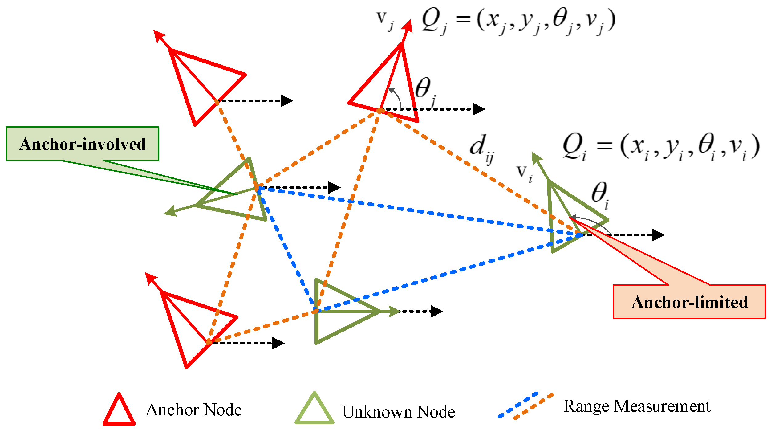
where $v_i^{(t)}$ and $w_i^{(t)}$ are the linear velocity and angular velocity of node i at time step t, respectively; ${\theta }_i^{(t)}$ is the azimuth angle between the node i and the positive x-axis of the navigation coordinates (see Figure 1); T is the time interval between two time steps.

In theory, we can calculate the current position of the node using the velocity and navigation direction information. This method is known as dead reckoning (DR). However, the accumulated error caused by the inertial device reduces the positioning accuracy of it. Thus, this paper will focus on the influence of course angle cumulative error on positioning.

2.2. Measurement Models

For UAV i in this network, inertial measurements $I_i^{(t)}=\{{\widehat{v}}_i^{(t)},{\widehat{\theta }}_i^{(t)}\}$ are often used to predict the position of unknown nodes. The measurement models of them are as follows:

$$\begin{array}{cc}\hfill {\widehat{v}}_i^{(t)}& =v_i^{(t)}+{\mu }_i^{(t)},i\in \xi ,\hfill \end{array}$$

(2)

$$\begin{array}{cc}\hfill {\widehat{\theta }}_i^{(t)}& ={\theta }_i^{(t)}+{\displaystyle \sum _{\tau =1}^t}{\zeta }_i^{(\tau )},i\in \xi ,\hfill \end{array}$$

(3)

where ${\mu }_i^{(t)}$ and ${\zeta }_i^{(t)}$ are measurement noise of speed and heading angle, respectively. Both of them follow Gaussian distributions with variances ${\sigma }_{v,i}^2$ and ${\sigma }_{\theta ,i}^2$.

Assuming that $\forall i\in \xi$ receives two types of measurement information, one comes from anchor nodes, and another is from unknown nodes. According to the triangulation principle, in a dynamic 2D UAV network, an unknown node needs at least three nearby anchors to determine its position. Therefore, for nodes with few nearby anchor nodes in the network, which are in the anchor-limited scenario as shown in Figure 1, how to make full use of the cooperation information between different nodes and quantify the credibility of the information is the key to improving the accuracy of localization estimation.

The distance-measurement model can be expressed as

$${\widehat{d}}_{ij}^{(t)}=g(q_i^{(t)},q_j^{(t)})=∥q_i^{(t)}-q_j^{(t)}∥+{\eta }_{ij}^{(t)},j\in {{\rm Y}}_i,$$

(4)

where ${\widehat{d}}_{ij}^{(t)}$ indicates the measured distance among the nodes, $g(·)$ is the measurement function, and $\parallel ·\parallel$ is the Euclidean norm. Considering that ranging is usually time-of-arrival-based, ${\eta }_{ij}$ is the measurement noise following a zero-mean Gaussian distribution with covariance $\gamma$ [31]. Moreover, the real-time distance-measurement vector of UAV i to the surrounding communicable nodes is expressed as $D_i^{(t)}=\{{\widehat{d}}_{ij}^{(t)}:i\in \xi ,j\in {{\rm Y}}_i\}$.

3. Bayesian Estimation

In this section, given the measurement results mentioned above, the positions can be estimated by Bayesian estimators. This paper estimates the position by designing a minimum mean square error (MMSE) estimator:

$${\widehat{q}}_{i,MMSE}^{(t)}=\int q_i^{(t)}P(q_i^{(t)}|I_i^{(1:t-1)},D_i^{(1:t)})d{q}_i^{(t)},i\in \xi ,$$

(5)

where $I_i^{(1:t-1)}=\{{\widehat{v}}_i^{(1:t-1)},{\widehat{\theta }}_i^{(1:t-1)}\}$ denotes inertial measurement information at time step 1 to $t-1$, and where $D_i^{(1:t)}$ denotes distance-measurement information at time step 1 to t. It can be seen from (5) that the key step is to calculate the posterior probability density function (PDF) $P(q_i^{(t)}|I_i^{(1:t-1)},D_i^{(1:t)})$. And it can be expressed as

$$\begin{array}{c}\hfill P(q_i^{(t)}|I_i^{(1:t-1)},D_i^{(1:t)})={\displaystyle \frac{1}{\varrho }}P(D_i^{(t)}|q_i^{(t)})P(q_i^{(t)}|I_i^{(1:t-1)},D_i^{(1:t-1)}),i\in \xi ,\end{array}$$

(6)

where $\varrho$ is a normalization factor that is treated as a constant during inference, ensuring that the integral of the posterior distribution is 1. It is expressed as

$$\begin{array}{cc}\hfill \varrho & =P(D_i^{(t)}|I_i^{(1:t-1)},D_i^{(1:t-1)})\hfill \\ \hfill & =\int P(D_i^{(t)}|q_i^{(t)})P(q_i^{(t)}|I_i^{(1:t-1)},D_i^{(1:t-1)}).\hfill \end{array}$$

(7)

The prior probability in (6) is represented as follows:

$$\begin{array}{c}\hfill P(q_i^{(t)}|I_i^{(1:t-1)},D_i^{(1:t-1)})=\int P(q_i^{(t)}|q_i^{(t-1)})P(q_i^{(t-1)}|I_i^{(1:t-1)},D_i^{(1:t-1)})d{q}_i^{(t-1)}.\end{array}$$

(8)

In this paper, it should be noted that the distance-measurement values $d_{ij}$ and $d_{ji}$ are not equal, due to the use of different range sensors. In other words, the information exchanged between the two nodes is independent. Therefore, the likelihood function in (6) can be expressed as

$$P(D_i^{(t)}|q_i^{(t)})=\prod _{i\in \xi ,j\in {{\rm Y}}_i}p({\widehat{d}}_{ij}^{(t)}|q_j^{(t)},q_i^{(t)}).$$

(9)

From Formulas (5)–(9), we can obtain the complete posterior calculation as follows:

$$\begin{array}{c}\hfill P(q_i^{(t)}|I_i^{(1:t-1)},D_i^{(1:t)})={\displaystyle \frac{{\displaystyle \prod _{i\in \xi ,j\in {{\rm Y}}_i}}p({\widehat{d}}_{ij}^{(t)}|q_j^{(t)},q_i^{(t)})·P(q_i^{(t)}|I_i^{(1:t-1)},D_i^{(1:t-1)})}{\varrho }},i\in \xi .\end{array}$$

(10)

Thus, with the help of Bayesian estimation, we can use the information of unknown nodes and anchor nodes to calculate the position of every UAV in the network. However, due to the complex parameter space, obtaining accurate continuous posterior distributions is difficult in real situations. Therefore, the particle-based method is used to estimate the location of the UAV in this paper.

4. The Proposed Cooperative Localization Algorithm

4.1. Overview

In this section, an adaptive Wasserstein filter (AWF) with distance-constrained bare bones self-recovery particles (CBBP) is proposed. The algorithm flowchart is shown in Figure 2. three innovative works were carried out as follows: First, by fusing the sensor information of the INS and TOA, this paper designed transition particles for prior particle initialization by using historical estimation information instead of directly using inertial measurements, which helps to suppress the negative impact of INS cumulative errors on localization performance. Then, the distance measurements between the UAV and neighbor nodes were used to update the particle weights, and the Wasserstein distance likelihood function based on slice segmentation was designed to fully quantify the difference between the observed and the prior data. Finally, a particle diversity index based on Gini purity was designed to judge the generation of the particle poverty problem, and the bare bones particles with distance constraints were used to pull the outlier particles to move to the high-likelihood region to achieve more robust and accurate positioning.

4.2. The Design of Prior

For the AWF algorithm proposed in this paper, the primary purpose of the prior design was to suppress the cumulative error generated by inertial components and ensure the quality of the particles, to avoid particle degradation.

As shown in Figure 3, the blue and black polylines represent the posterior estimated and actual trajectories in n time steps, respectively. Evidently, the azimuth information (brown polyline) output by the INS has deviated from the ground truth at time step $t-1$. If the prior particles are generated directly from the INS data of the previous time step, the ground truth cannot be overwritten. In other words, the increasing cumulative error increases the uncertainty of the error, which seriously affects the quality of the prior particle. To solve this problem, inspired by [32], transition particles (the green crosses) were designed, using the historical estimated information between time steps $t-n$ and $t-1$. When the navigation time was extended, the error uncertainty at time $t-n$ was smaller than at time $t-1$. Considering this feature, we used the historical estimation information (heading angle and distance) at time $t-n$ and time $t-1$ to sample particles and obtain transition particles. Based on the transition particles, a set of prior particles was obtained based on the angle and velocity information of the last time step from the INS. Compared with directly using inertial measurements to initialize the prior particles, the inertial-measurement-processing strategy designed in this paper can cover the ground truth of the UAV in the case of sizeable cumulative error, which provides a more significant information gain for the positioning of the UAV in an anchor-limited environment.

Additionally, the closer $t-n$ is to the initial time, the less affected the historical estimation information will be by the cumulative error, but the space complexity will increase accordingly. Therefore, the setting of n is set according to the size of the actual computing resources to achieve the trade-off between space complexity and the accuracy of the algorithm.

Assume that at time t there is a group of particles ${\Omega }_i^{(t)}={\{q_{i,k}^{(t)},w_{i,k}^{(t)}\}}_{k=1}^K$ located at the UAV i, where K is the number of particles and $w_{i,k}^{(t)}$ is the weight of $q_{i,k}^{(t)}$. The formula for position prediction is as follows:

$$\begin{array}{cc}\hfill q_{pri,k,i}^{(t)}& =q_{final,i}^{(t-n)}+d_{k,i}[cos({\theta }_{k,i});sin({\theta }_{k,i})]\hfill \\ \hfill & +v_{k,i}^{(t-1)}T[cos({\theta }_{k,i}^{(t-1)});sin({\theta }_{k,i}^{(t-1)})],\hfill \\ \hfill d_{k,i}& \sim N(\parallel q_{final,i}^{(t-n)},q_{final,i}^{(t-1)}\parallel ,{\beta }_i^t),\hfill \\ \hfill {\theta }_{k,i}& \sim U(\Psi (q_{final,i}^{(t-n)},q_{final,i}^{(t-1)})-0.5{\alpha }_i^t,\hfill \\ \hfill & \Psi (q_{final,i}^{(t-n)},q_{final,i}^{(t-1)})+0.5{\alpha }_i^t),\hfill \\ \hfill v_{k,i}^{(t-1)}& \sim N({\widehat{v}}_i^{(t-1)},{\sigma }_{v,i}^{{(t-1)}^2}),\hfill \end{array}$$

$$\begin{array}{cc}\hfill {\theta }_{k,i}^{(t-1)}& \sim N({\widehat{\theta }}_i^{(t-1)},{\sigma }_{\theta ,i}^{{(t-1)}^2}),\hfill \end{array}$$

(11)

$$\begin{array}{cc}\hfill w_{pri,i,k}^{(t)}& ={\displaystyle \frac{1}{K}},\hfill \end{array}$$

(12)

where $q_{final,i}^{(t-n)}$ represents the posterior estimate position of UAV i at time step $t-n$. ${\beta }_i^t$ can be set based on the magnitude of the accumulated errors. $\Psi (·)$ represents the heading angle between two points, and ${\alpha }_i^t$ controls the distribution range of the particles. T is the duration between two time steps. The variance ${\sigma }_{\theta ,i}^{{(t-1)}^2}$ increases with time, to simulate the growth of uncertainty caused by cumulative error.

4.3. The Design of the Likelihood Function

In this step, likelihood functions were designed to quantify the difference between real-time measurements and prior values in a dynamic network.

Considering that the prior distribution exists in the form of particles, this paper adopted approximate Bayesian inference and constructed a kernel density estimation (KDE) function [33] to reduce the computational cost. The function is shown below:

$$\begin{array}{cc}\hfill P(D_i^{(t)}|q_i^{(t)})& ={\displaystyle \frac{1}{\epsilon \sqrt{2\pi }}}exp(-{\displaystyle \frac{d_w{({\widehat{D}}_i^{(t)},D_{pri,i}^{(t)})}^2}{2{\epsilon }^2}}),\hfill \end{array}$$

(13)

where $\epsilon$ is the width factor that determines the concentration of the posterior distribution following the approximate Bayesian update within the range of $[0,1]$. Its value depends on the noise variance of the distance measurement [34]; $d_w(·)$ is the distance measurement of the similarity between the experimental observed data ${\widehat{D}}_i^{(t)}=[{\widehat{d}}_{i1}^{(t)},{\widehat{d}}_{i2}^{(t)},\dots ,{\widehat{d}}_{i{N}_i}^{(t)}]$ and the prior model data $D_{pri,i}^{(t)}=[d_{pri,i1}^{(t)},d_{pri,i2}^{(t)},\dots ,d_{pri,i{N}_i}^{(t)}]$. $N_i=card({{\rm Y}}_i)$ denotes the number of nodes near the UAV i.

To effectively screen prior particles, it is necessary to establish a distance measure that can accurately capture the difference between different distributions and be robust to local sensor measurement outliers. Due to its compliance with trigonometric inequality and the additivity principle, the Wasserstein distance serves as a reliable distance measure.

Therefore, the Wasserstein distance was introduced to evaluate the differences between the data. The mathematical definition formula is expressed as follows:

$$d_w(p_r,p_g)={(\underset{\kappa \in \prod (p_r,p_g)}{inf}{\int }_{\chi \times \chi }{∥x-y∥}^{p}d\zeta (x,y))}^{1/p},p\ge 1,$$

(14)

where $\prod (p_r,p_g)$ is the set of joint probability distributions $\zeta$ on $\chi \times \chi$, satisfying $\kappa (A\times \chi )=p_r(A)$ and $\zeta (\chi \times B)=p_g(B)$ for any $A,B\subseteq \chi$. For any joint probability distribution $\zeta (x,y)$, corresponding data x and y can be obtained through sampling; p is the parameter space dimension, and the norm $∥x-y∥$ quantifies the cost information of moving unit probability mass from x to y. In other words, $d_w(p_r,p_g)$ represents the minimum cost required to configure $p_r$ as the probability mass distribution of $p_g$.

To avoid the combination explosion problem and improve computational efficiency, this paper uses the method of slice segmentation to calculate the Wasserstein distance [35]. The mathematical description is as follows:

$$S{d}_w(p_r,p_g)={\int }_{S^{d-1}}{d_w}^p({p_r}_{\#}^{*}{p}_r,{p_r}_{\#}^{*}{p}_g)d\sigma (p_r),$$

(15)

where $S^{d-1}=\{p_r\in R_d:\parallel p_r{\parallel }_2=1\}$ denotes the d-dimensional unit sphere; ${p_r}^{*}$ is the linear form associated with $p_r$, and it satisfies $\forall y\in Y,{p_r}^{*}(y)=\langle p_r,y\rangle$; $\langle ·,·\rangle$ denotes the Euclidean inner product; $\sigma$ is the uniform distribution on $S^{d-1}$, and, for any measurable function $f:Y\leftarrow R,\varpi \in P(Y)$, $f_{\#}\varpi$ is defined as $\forall A\in B(R),f_{\#}\varpi =\varpi (f^{-1}(A))$, with $f^{-1}(A)=\{y\in Y:f(y)\in A\}$.

4.4. Weight Calculation and Position Estimation

Based on the above prior particles and likelihood function, the next goal was to obtain the posterior probability and to calculate the position of the UAVs. This paper used importance sampling to first draw K particles ${\{q_{p,i,k}^{(t)}\}}_{k=1}^K$ from the proposal distribution $q(·)$, and then each particle was weighted. The weight of each particle was calculated as follows:

$$w_{p,k,i}^{(t)}\propto {\displaystyle \frac{P(D_i^{(t)}|q_{p,k,i}^{(t)})P(q_{p,k,i}^{(t)}|I_i^{(1:t-1)},D_i^{(1:t-1)})}{\widehat{q}(q_{p,k,i}^{(t)})}}{w}_{p,k,i}^{(t-1)}.$$

(16)

In this paper, we chooe the prior as the proposal distribution, so the process of inference can be seen as reweighting the prior particles ${\{q_{pri,i,k}^{(t)}\}}_{k=1}^K$.

The resulting posterior particles were normalized as follows:

$$w_{p,k,i}^{(t)}=\frac{w_{p,k,i}^{(t)}}{{\sum }_{k=1}^K{w}_{p,k,i}^{(t)}}.$$

(17)

For the PF algorithm, resampling was the key to avoiding particle degradation. To reduce the computational cost and reduce the sampling bias, residual systematic resampling (RSR) [36] was used as the resample protocol in this paper.

In general, after the particle resampling, the set of posterior particles ${\Omega }_{final,i}^{(t)}={\{q_{final,i,k}^{(t)},w_{final,i,k}^{(t)}\}}_{k=1}^K$ for the UAV i in the network at time step t is obtained:

$${\widehat{q}}_{i,MMSE}^{(t)}={\displaystyle \sum _{k=1}^K}{w}_{final,i,k}^{(t)}{q}_{final,i,k}^{(t)}.$$

(18)

However, since the essence of resampling is to replace the small-weight particles by copying the large-weight particles, most of the particles in the filtering algorithm after multiple frames come from the same particle ancestor, and the sample diversity is lost.

Therefore, it is necessary to judge whether the particle impoverishment problem occurs. The particle self-recovery algorithm designed in this paper will be introduced in Section 4.5. Our AWF-CBBP algorithm is presented in Algorithm 1:

Algorithm 1 The Proposed AWF-CBBP Algorithm

Initialize:   $q_i^{(0:t-1)},\forall i\in \xi$ Receive the inertial measurements at time step t. for $k=1$ to K do    Draw prior particles ${\Omega }_i^{(t)}={\{q_{pri,i,k}^{(t)},w_{pri,i,k}^{(t)}\}}_{k=1}^K$ as in (11).    Calculate the distance vector $D_{pri,i}^{(t)},j\in {{\rm Y}}_i$.    Receive the real-time observation ${\widehat{D}}_i^{(t)}$ from neighbors.    Calculate the sliced Wasserstein distance $S{d}_w(D_{pri,i}^{(t)},{\widehat{D}}_i^{(t)})$ as in (15).    Calculate the likelihood function $P(D_i^{(t)}|q_i^{(t)})$ as in (13).    Update the particle weights $w_{p,k,i}^{(t)}$ as in (16). end for Normalize the weights and obtain the final set ${\Omega }_{final,i}^{(t)}$. Calculate the particle diversity index $G{I}_i^{(t)}$ as in (19). if $G{I}_i^{(t)}<\gamma$ then    Enter the particle self-recovery algorithm. $\leftarrow \mathbf{Algorithm}$ 2 else    Residual Systematic Resampling to update the weights. end if Calculate the new position estimation ${\widehat{q}}_{i,MMSE}^{(t)}$ as in (18).

Algorithm 2 Bare Bones Particle Self-recovery Algorithm with Distance Constraint

Input:${\{q_{p,k,i}^{(t)},w_{p,k,i}^{(t)}\}}_{k=1}^K,{\{d_{w,k}^{(t)}\}}_{k=1}^K$ output: ${\{q_{new,k,i}^{(t)},w_{new,k,i}^{(t)}\}}_{k=1}^K$ Calculate the mean $\zeta$ and the mean ${\overline{d}}_w^{(t)}$ of the set ${\{d_{w,k}^{(t)}\}}_{k=1}^K$. Determine the confidence bounds $s_1$ and $s_2$. for $k=1$ to K do    if $d_{w,k}^{(t)}<s_1$ then      $N_l=N_l+1$    else if $d_{w,k}^{(t)}>s_2$  then      $N_s=N_s+1$    else      $N_m=N_m+1$    end if end for for $l=1$ to $N_l$ do    while $d_{w,l}^{(t)}>s_2$ and $num<ma{x}_{iter}$ do      $num=num+1$      Randomly draw the position $q_{best,rand}^{(t)}$ of an important particle.      Update the position $q_{new,i,l}^{(t)}$ of the particle l as in (22).      Calculate the new distance $d_{w,l}^{(t)}$.      if $d_{w,l}^{(t)}<s_1$ and $N_{l,new}<\rho K$ then         $N_{l,new}=N_{l,new}+1$      else if $s_2<d_{w,l}^{(t)}<s_1$ and $N_{m,new}<(1-\rho )K$ then         $N_{m,new}=N_{m,new}+1$      end if    end while end for Assign the weights of the particles as in (23).

4.5. Particle Self-Recovery Strategy

When recovering the position of a particle, two challenges need to be addressed: (1) How do we specify a reasonable criterion for particle impoverishment? (2) How can a self-recovery algorithm be designed to achieve the trade-off between time and accuracy?

To solve these problems, for this section, a particle diversity index based on Gini purity is proposed, and a bare bone particle self-recovery algorithm with distance constraint (CBBP) was designed to pull ill particles to move to the high-likelihood region to alleviate the particle poverty problem.

4.5.1. Design of Particle Diversity Index Based on Gini Purity

In information theory, Gini purity is a tool to divide data purity, and the value is distributed between 0 and 1. The smaller the Gini purity, the higher the data purity. In the process of collaborative localization, the higher the degree of particle diversity, the lower the data purity, and the closer the Gini purity is to 1. On the contrary, when most particles fall into the same interval, particle diversity is at its lowest, and the corresponding Gini purity is more minor.

Given this feature, the change of Gini purity is used to determine whether the particle recovery operation is carried out. For the particle set representing UAV i at time step t, the particle diversity index based on Gini purity is calculated as follows:

$$G{I}_i^{(t)}={\displaystyle \sum _{k=1}^K}\sum _{k^{\prime }\ne k}{p}_k{p}_k^{\prime }=1-{\displaystyle \sum _{k=1}^K}{p}_k^2.$$

(19)

For the particle weight set ${\{w_{p,i,k}^{(t)}\}}_{k=1}^K=\{w_{p,i,1}^{(t)},w_{p,i,2}^{(t)},\dots ,w_{p,i,K}^{(t)}\}$ obtained after importance sampling, take $w_{min}=min\{w_{p,i,1}^{(t)},w_{p,i,2}^{(t)},\dots ,w_{p,i,K}^{(t)}\}$, $w_{max}=max\{w_{p,i,1}^{(t)},w_{p,i,2}^{(t)},\dots ,w_{p,i,K}^{(t)}\}$. Divide the observation interval $[w_{min},w_{max}]$ into K cells with the same width, and count the number of particles ${\{w_{p,i,k}^{(t)}\}}_{k=1}^K$ falling into each cell $n_k(k=1,2,\dots ,K)$, and ${\sum }_{k=1}^K{n}_k=K$. The following formula can be obtained:

$$p_k=\frac{n_k}{K}.$$

(20)

Set $\gamma$ as the acceptable diversity factor threshold. When $G{I}_i^{(t)}<\gamma$, it means that the diversity of particles is too low compared with the previous cycle, which is prone to the problem of particle poverty. It is necessary to enter the self-recovery algorithm to adjust the particle combination weight.

4.5.2. Bare Bones Particle Self-Recovery Algorithm with Distance Constraint

When the impoverishment problem of the particle set is detected, the sampling process in the filtering at that time is transformed into an intelligent sampling process, and the outlier particle set is guided to the high-likelihood region to restore the performance of the filtering algorithm. In this paper, a self-recovery algorithm based on bare bones particles with distance constraint is proposed.

In the above likelihood function design part, we can obtain the Wasserstein distance set of particle set ${\{d_{w,k}^{(t)}\}}_{k=1}^K=\{d_{w,1}^{(t)},d_{w,2}^{(t)},\dots ,d_{w,K}^{(t)}\}$; the variance is $\zeta$ and the mean is ${\overline{d}}_w^{(t)}$. Let $s_1=\overline{d_w^{(t)}}-\zeta$, $s_2=\overline{d_w^{(t)}}+\zeta$, and divide the particles into three categories, and their mathematical expressions are as follows:

$$\begin{array}{cc}\hfill & {\Omega }_i^{(t)}={\Omega }_{i,s}^{(t)}\cup {\Omega }_{i,m}^{(t)}\cup {\Omega }_{i,l}^{(t)}\hfill \\ \hfill & s.t.\left\{\begin{array}{c}{\Omega }_{i,s}^{(t)}={\{(q_{i,k}^{(t)},w_{i,k}^{(t)}),d_{w,k}^{(t)}>s_2\}}_{k=1}^{N_s}\hfill \\ {\Omega }_{i,m}^{(t)}={\{(q_{i,k}^{(t)},w_{i,k}^{(t)}),s_1<d_{w,k}^{(t)}<s_2\}}_{k=1}^{N_m}\hfill \\ {\Omega }_{i,l}^{(t)}={\{(q_{i,k}^{(t)},w_{i,k}^{(t)}),d_{w,k}^{(t)}<s_1\}}_{k=1}^{N_l}\hfill \end{array}\right.\hfill \end{array}.$$

(21)

K particles are divided into three levels by two confidence levels based on Wasserstein distance. Among them, $N_s$ particles have larger distance measures, smaller weights, and lower particle quality, which are called outlier particles. $N_m$ particles have moderate weight and good stability, which are suitable for direct retention and are called moderate particles. $N_l$ particles with higher weight will be retained and used as the "benchmark" to guide outlier particles, which are called important particles.

After dividing the particle set, the next step is to formulate a reasonable particle guidance rule to retain the particles’ diversity and have an acceptable time cost. Inspired by bare bones particle swarm (BBPS) [37], a distance-constrained BBPS update rule is formulated as follows:

$$\begin{array}{cc}\hfill q_{new,i,k}^{(t)}& \sim N({\mu }_{new},{\sigma }_{new}^2),\hfill \\ \hfill {\mu }_{new}& =\frac{1}{T_k}{q}_{i,k}^{(t)}+\frac{T_k-1}{T_k}{q}_{best,rand}^{(t)},{\sigma }_{new}^2=∥q_{i,k}^{(t)}-q_{best,rand}^{(t)}∥,\hfill \end{array}$$

(22)

where $T_k=1+lo{g}_2^{d_{w,k}}$ is the adaptive weight factor, which introduces the distance constraint. The greater the distance between the prior value and the observed value, the worse the quality of the particle, and then the average value is more biased towards the random important particle, which ensures that the particle moves to the high-likelihood region while retaining the rich estimation uncertainty of the particle; $q_{best,rand}^{(t)}$ denotes the coordinate of a particle randomly drawn from the set of important particles. The random sampling operation adds random disturbance to the parameters of Gaussian distribution, which helps to avoid falling into the local minimum.

If the newly generated particle falls into the geometric region of interest (moderate or important particle) and meets $N_{l,new}<\rho K$ and $N_{m,new}<(1-\rho )K$, the new particle successfully settles down; otherwise, continue to the previous step; $\rho$ represents the largest proportion of important particles.

If there are still a few particles that have not reached the high-likelihood region after exceeding the maximum number of iterations $N_{iter}$, the particles are retained to ensure that the total number of particles remains unchanged, expressed as set ${\Omega }_{i,res}^{(t)}$ and $card({\Omega }_{i,res}^{(t)})=N_{res}$. They are passed together with the updated set of particles to the next moment.

The updated particle set ${\Omega }_{i,new}^{(t)}={\Omega }_{i,res}^{(t)}\cup {\Omega }_{i,m,new}^{(t)}\cup {\Omega }_{i,l,new}^{(t)}$ contains three types of particles: moderate particles, important particles, and residual particles. Reassign the weight to the updated particles, retain the original weight for the moderate particles and residual particles before the update, and reassign the weight to the particles leading to the high-likelihood area and the important particles before the update as follows:

$$w_{new,i,k}^{(t)}=\frac{1}{K-(N_{res}+N_l)},$$

(23)

where $N_l$ is the number of important particles before self-recovery. The self-recovery algorithm is described in Algorithm 2.

5. Numerical Simulation

5.1. Simulation Setup

In the 500 m × 500 m area, there are three UAVs $R_1$, $R_2$, $R_3$ and three anchor nodes, respectively. To establish a cooperative environment, two different communication rules were designed as follows:

(1) Anchor-involved scenario: Three UAVs can communicate with three anchors anytime. In other words, the UAV has sufficient observation information to suppress the negative impact of INS cumulative error on positioning performance.

(2) Anchor-limited scenario: Three UAVs can only communicate with the nearest anchor point. That is to say, in the two-dimensional space, the UAV cannot achieve localization with less than three anchors, so it is in a harsh positioning environment. It must complete the positioning with the help of the cooperative information of other UAVs.

The algorithm’s performance is assessed in two classical moving-trajectory scenarios: straight line and curve. The UAV moves 50 s at the speed of 8 m/s, the sampling interval is 2 s, and the velocity noise variance is (2 m/s)². The measurement noise variance of the range is (5 m)². In the straight-line scenario, the azimuth angles of the three nodes are set to 15°, 45°, and 75°, respectively; in the curve scenario, the node angular velocity varies uniformly, the noise variance is 1, and the initial heading angles are 180°, 60°, and 300°, respectively.

Set the number of particles to 500 and perform 1000 Monte Carlo simulations under the hardware configuration of AMD Ryzen 7 PRO 4750U 1.7 Ghz and 16 GB memory. The positioning accuracy of different algorithms is compared by comparing Euclidean distance error and the root mean square error (RMSE), which are calculated as follows:

$$DistanceError={\displaystyle \frac{1}{M}}{\displaystyle \sum _{i=1}^M}\sqrt{\left|\right|{\widehat{q}}_{i,MMSE}^{(t)}-q_{i,true}^{(t)}\left|\right|}{)}^2,$$

(24)

$$RMSE=\sqrt{{\displaystyle \frac{1}{\tau }}{\sum }_{t=1}^{\tau }{(DistanceError)}^2},$$

(25)

where $\tau$ is the time step of UAV i, M is the number of the UAVs, ${\widehat{q}}_{i,MMSE}^{(t)}$ is the estimated position, and $q_{i,true}^{(t)}$ is the true reference position of the UAV i at that time step t.

5.2. Comparison of the Cooperative Localization Approaches

To assess the performance of the proposed algorithm, the following localization approaches are compared in the anchor-involved environment:

(1) DR: The attitude and velocity information of the INS and the dynamic model are used for positioning, and the cooperation information between UAVs is not used.

(2) Particle filter cooperative localization (PF-CL): The probability sampling is completed by using the position estimation at the last moment and the sensor data of the INS, and the position estimation is refined by sensor fusion and resampling to achieve accurate coordination.

(3) Optimal weighted-particle filter (OWPF) [22]: The positioning accuracy is improved by assigning optimal weights to particles to achieve weighted resampling and iterative updating.

(4) Error-ellipse-resampling particle filter (EER-PF) [26]: The error ellipse is used to set different confidence levels to realize the hierarchical resampling optimization based on particle position, and the state estimation optimization method based on spatial distance constraint is designed to realize the collaborative tracking and fusion of spatiotemporal information.

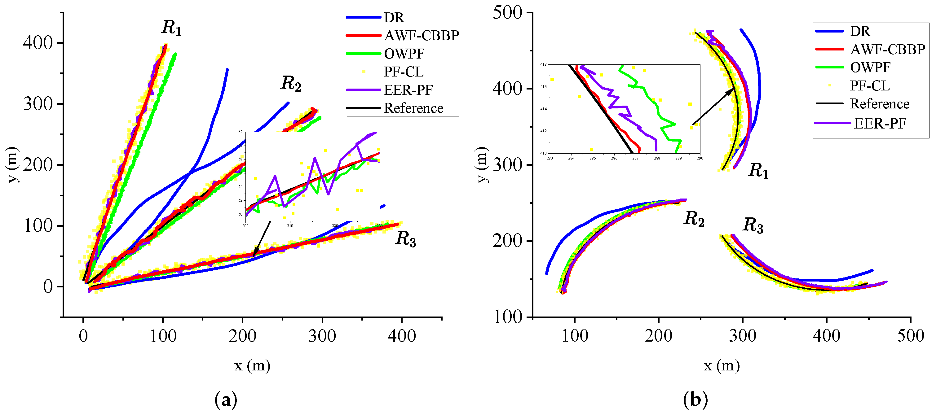
As shown in Figure 4, the UAV moves along two typical trajectories: straight line and curve. The black line is the real trajectory, and various positioning trajectories are also shown in the figure. It can be seen intuitively that with the passage of time, the blue line gradually deviates from the ground truth, which also verifies that the error of DR shows an increasing trend over time due to the influence of the cumulative error of the inertial components. However, with the help of the absolute position information of the anchors, the positioning errors of several other algorithms, except DR, will not drift with time.

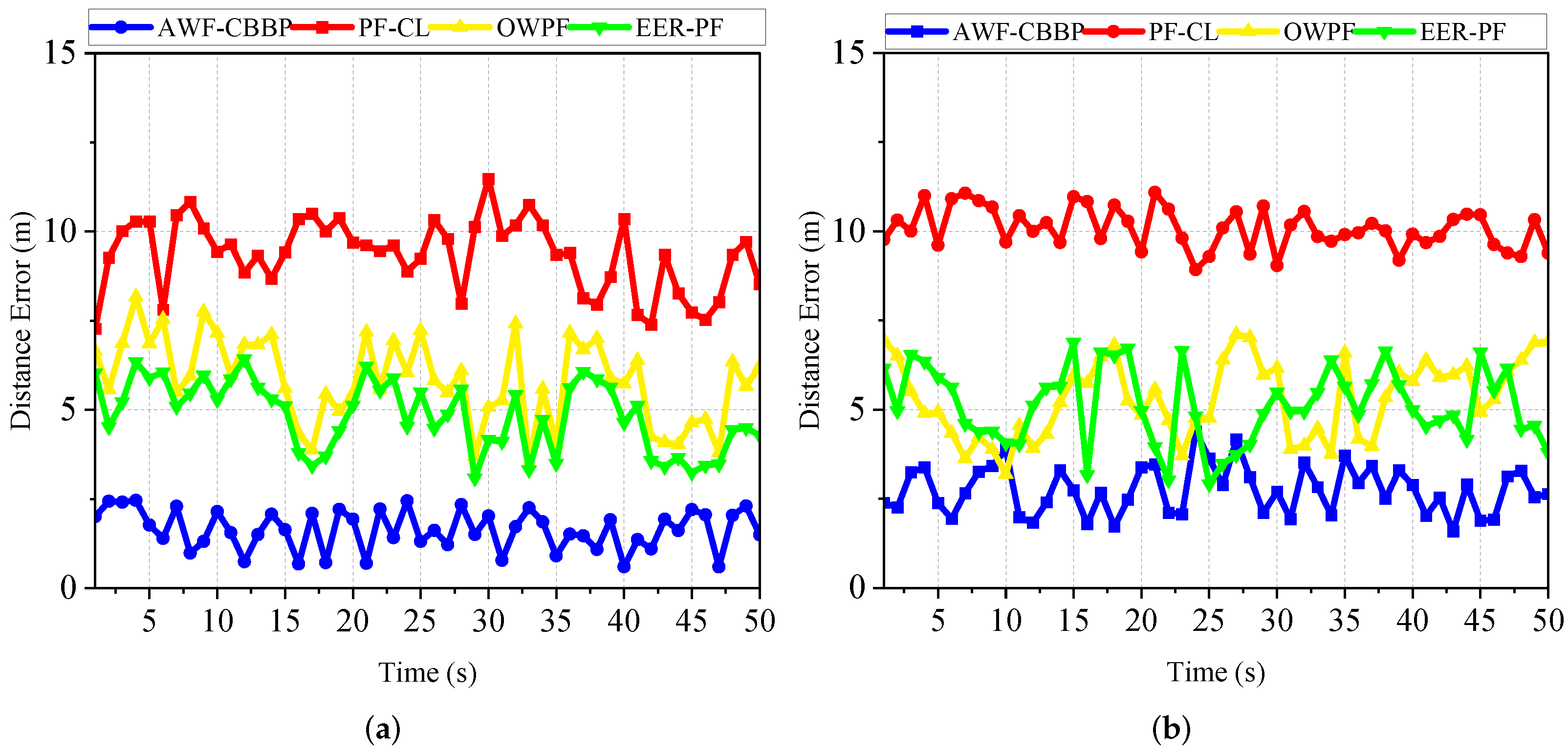
Figure 5 shows the error trends of each algorithm over time for two trajectories, line and curve. It is evident that the error in the straight scene is slightly smaller than that in the curved scene, which is due to the faster accumulation of errors due to the frequent attitude changes in the curved motion. Under the same trajectory, compared with other methods, the accuracy of the AWF-CBBP algorithm designed in this paper has been greatly improved. The traditional particle filter takes the sensor-detection data as the initial value of the position, and the quality of the prior knowledge directly affects the final estimated target position, so there is still much room for improvement. Compared with the conventional particle filter algorithm, OWPF uses the observation variance of different robots to quantify the ranging information reliability, but the lack of angle information and historical position information makes it unable to provide rich information gain, so the improvement is not enough. EER-PF uses the error ellipse to improve the resampling process and designs an INS/TOA fusion algorithm. However, the copy operation in the resampling stage may cause the particle poverty problem in the filtering algorithm with a small number of particles. The reason why the AWF-CBBP proposed in this paper can improve positioning accuracy can be explained from two aspects. On the one hand, the prior particles are obtained using the historical position-estimation data and inertial data fusion, which ensures that the particles have sufficient scalability based on covering the ground truth. On the other hand, this paper has designed a likelihood function based on the Wasserstein measure to fully quantify the difference between the real-time observation data and the prior data to obtain a convergent and accurate localization result. Experiments show that the proposed algorithm has better accuracy performance in both straight line and curve scenes.

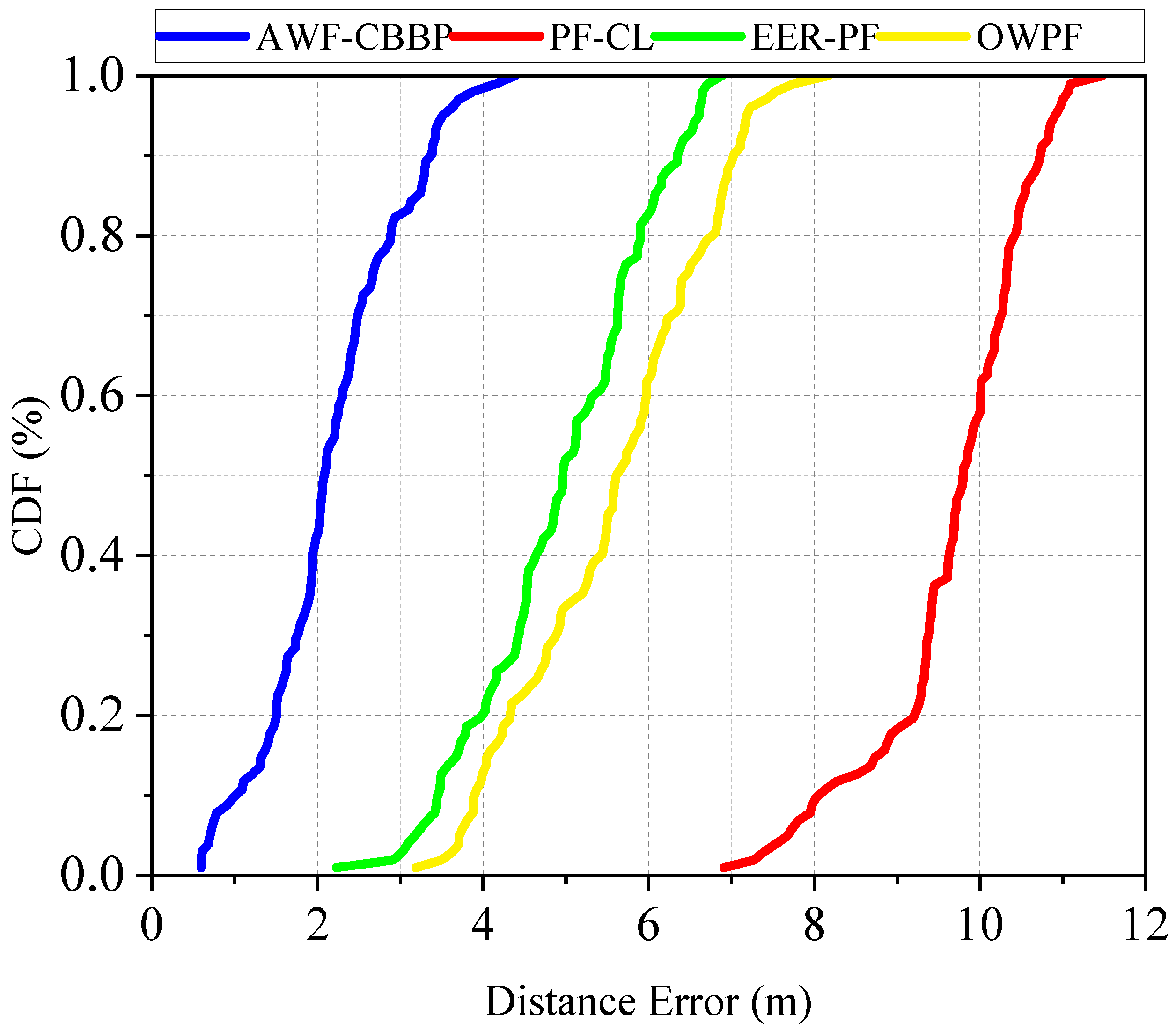
The error cumulative distribution function curves of different algorithms in the anchor-involved environment are shown in Figure 6. It can be seen that the proposed algorithm has a 50% probability error less than 2 m and a 98.5% probability error less than 4 m.

To objectively compare their computational complexity,

Table 1. Performance comparison of localization algorithms.

Algorithm	Max Error (m)	Min Error (m)	Avg Error (m)	Execution Time (s)
DR	79.56	11.57	44.98	0.0078
PF-CL	11.48	8.92	9.68	0.1162
OWPF	8.17	3.49	5.58	0.1683
EER-PF	6.88	3.08	4.95	0.1234
AWF-CBBP	4.38	0.60	2.38	0.2132

shows the corresponding computational time of several algorithms. It can be seen that DR takes the least time because it does not require measurements between UAVs and can be directly calculated from its velocity angle information. In contrast, Bayesian estimation using filtering requires more computing time. The AWF-CBBP algorithm designed in this paper achieves the most ideal positioning accuracy among several methods. However, the designed prior particle-generation strategy fusing historical information makes its execution time slightly higher, but it can still meet the requirements for real-time flight.

In conclusion, compared with other approaches, the proposed method has the smallest estimation error and significantly improves the positioning accuracy despite the increase of tolerable calculation, which validates the feasibility of the proposed method.

5.3. Effect of Distance Measurement on Localization Performance

To evaluate the effectiveness of the likelihood function based on the Wasserstein distance as proposed in this paper, we compared our algorithm with the commonly used Euclidean distance and KL divergence in the anchor-involved scenario.

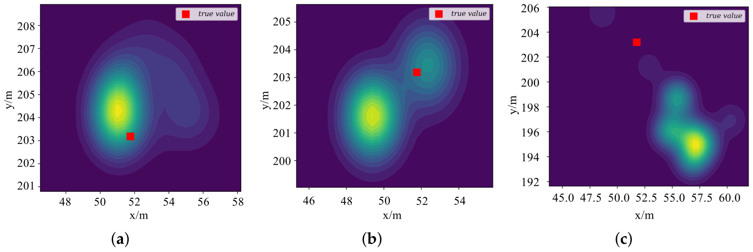
Under the same parameter setting, Figure 7 is the contour plot of the likelihood function for UAV R1 based on different measures in the curved trajectory of the anchor-involved scenario at the 20s. It can be seen that compared with the Euclidean distance and KL divergence, the Wasserstein distance measure significantly quantifies the difference between the observed and the prior data, updates the prior knowledge, and the converged particle positions maintain a high consistency with the ground truth. The KL divergence can become infinitely large when distributions do not overlap, whereas the Wasserstein distance can still measure differences even when the support sets of the distributions do not overlap. The prior and observation distributions can be significantly different in the actual situation, making the Wasserstein distance’s characteristic particularly crucial. Furthermore, the Wasserstein distance is less sensitive to outliers than the Euclidean distance. Outliers can distort the measurement of distribution differences, resulting in unreliable filtering outcomes. The Wasserstein distance mitigates this effect by considering the distribution’s overall shape and spread. In summary, the Wasserstein distance offers a more comprehensive and robust measure for quantifying distribution differences in particle filtering, particularly in scenarios with nonlinearity, non-overlapping support sets, and outliers.

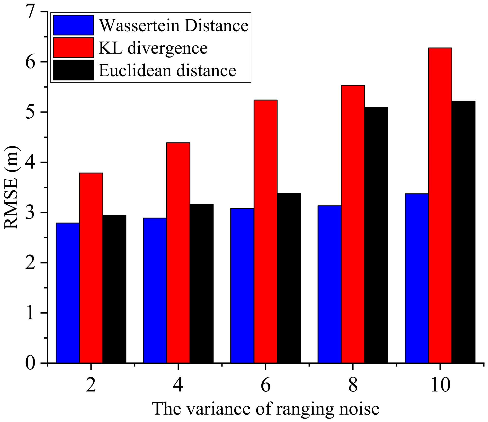
Now, we further discuss the influence of different distance measures on the localization accuracy under different noise variances. The root mean square error of the agents in the algorithms based on different distance measures is compared in Figure 8 for different ranging variances. It can be seen that as the noise variance increases, the localization error increases. However, the proposed AWF-CBBP algorithm has the highest accuracy and is less affected by the change of ranging variance, which indicates that the Wasserstein measure can better integrate measurement information to obtain sensor estimators that are closer to the ground truth and have better robustness against noise.

5.4. Evaluation of Particle Generation Strategies

In the above experiment, the information gain due to the anchor makes its localization error not diverge over time. In this section, to verify the effectiveness of the designed prior particle-generation strategy in suppressing the cumulative error, we will discuss the localization performance of the proposed algorithm in harsh environments. The motion trajectories and parameter settings of the three UAVs are consistent with the above. The difference is that they are in an anchor-limited communication environment, and cooperative information between the UAVs is needed to suppress the negative impact of the cumulative error on their positioning performance. In other words, the UAV can complete the cooperative localization with the help of the observation information between UAVs and the prior position information of nearby UAVs. High-quality prior particles play a key role in suppressing the cumulative error and ensuring the angle information gain.

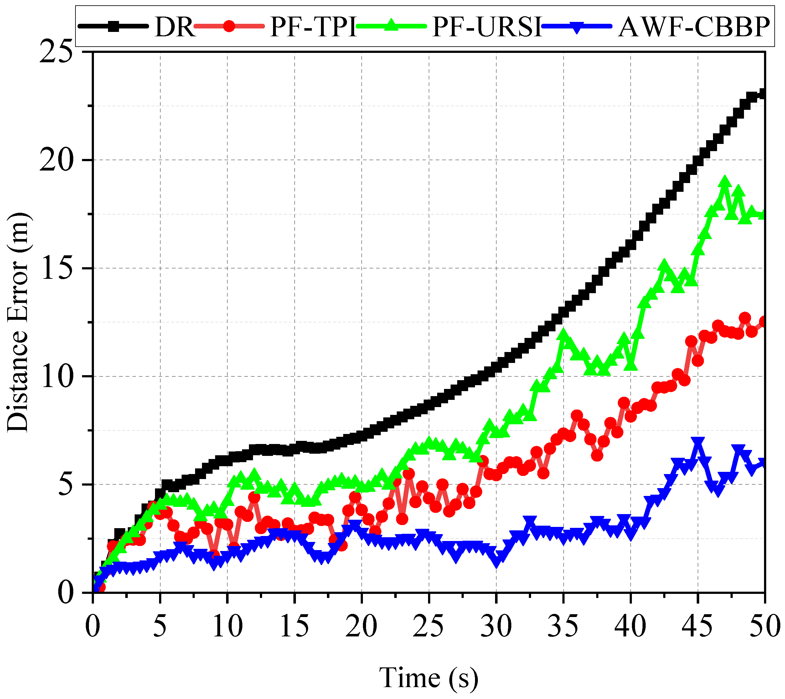
Three groups of experiments were designed to compare the performance of the particle filter algorithm using uniform random sampling initialization (URSI), the transition particle-based initialization (TPI) strategy, and the AWF-CBBP algorithm. Figure 9 illustrates the line plots of the localization errors of various localization algorithms over time in an anchor-limited environment. It can be seen that due to the lack of coordination information between the agents, the DR was affected by cumulative errors, and the errors kept increasing over time. Using the URSI strategy, the PF algorithm samples were based on the position information from the previous time. Although the cumulative error was suppressed under the constraint of the observation information, it still showed a large diffusion trend. When other parameters were unchanged, the initialization method of PF particles was replaced by the TPI strategy, and the historical information before the $t-n$ steps was fused. This indicates that the performance of the algorithm was a significant improvement compared with that of the traditional particle filter algorithm, which verifies the availability of the TPI strategy designed in this paper. Anyway, the proposed algorithm can maintain optimal accuracy performance.

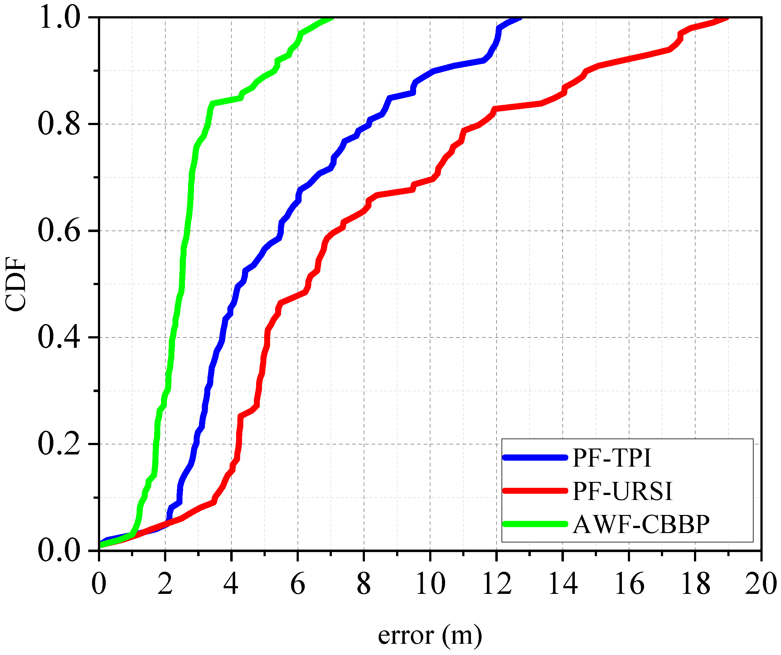
Figure 10 shows the root mean square error cumulative distribution function of the various positioning algorithms. It demonstrates that the positioning error of the AWF-CBBP algorithm proposed in this paper can still be less than 7 m in harsh environments. In contrast, the probabilities of error below 5m for PF-URSI and PF-TPI algorithms were only 40.4% and 56.6%, which confirms the advantages of the proposed algorithm in an anchor-limited environment.

5.5. Validation of Particle Self-Recovery Algorithm

To evaluate the effectiveness of the designed particle recovery algorithm, the performance of the algorithm in an anchor-involved scenario was compared with and without the self-recovery strategy. Considering the real-time flight requirements of a UAV swarm, the number of particle update iterations of the recovery algorithm should be manageable, and the judgment threshold of the particle poverty problem should be moderate. The maximum number of iterations $ma{x}_{iter}=3$ and the particle diversity threshold $\gamma =0.7$ were set. The maximum proportion $\rho$ of important particles was set to 0.6. Based on the above conditions, simulation experiments were carried out, to analyze and compare the average positioning performance of the UAVs.

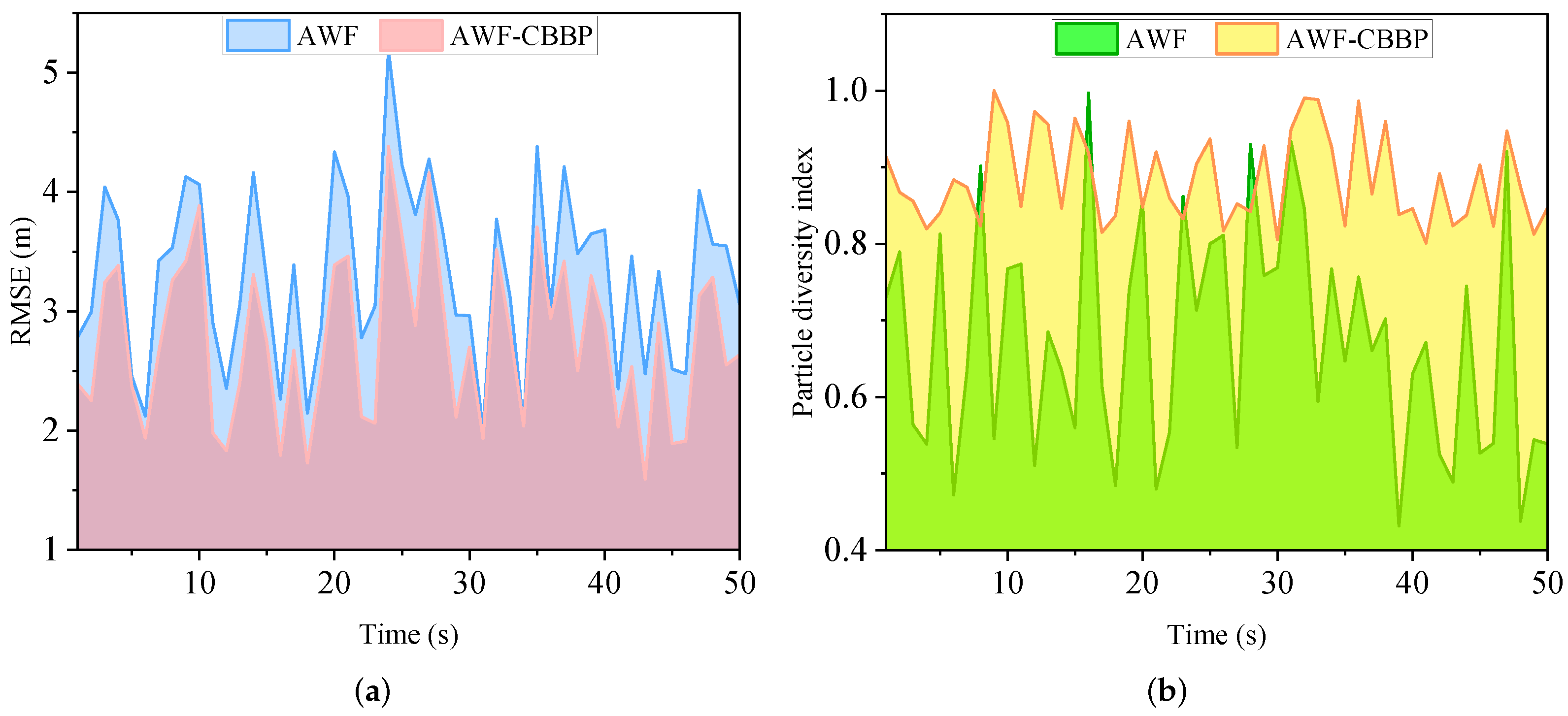
Figure 11 shows the trend of the RMSE and particle diversity index over time during the movement of the agent. It can be seen that the algorithm with a self-recovery strategy could maintain good diversity in the whole movement process. In contrast, for the algorithm without self-recovery, there were 22 times when the diversity factor was lower than 0.6, indicating that the self-recovery algorithm effectively alleviates the particle impoverishment problem. Regarding positioning accuracy, the positioning performance of the algorithm with a self-recovery strategy was $20.1\%$ higher than that of the algorithm without this strategy, which achieved a particular advantage. In summary, compared with AWF, the AWF-CBBP algorithm achieved better positioning accuracy while maintaining better particle diversity. This shows that the particle self-recovery algorithm designed in this paper can effectively guide outlier particles to move to the high-likelihood region without falling into a local minimum.

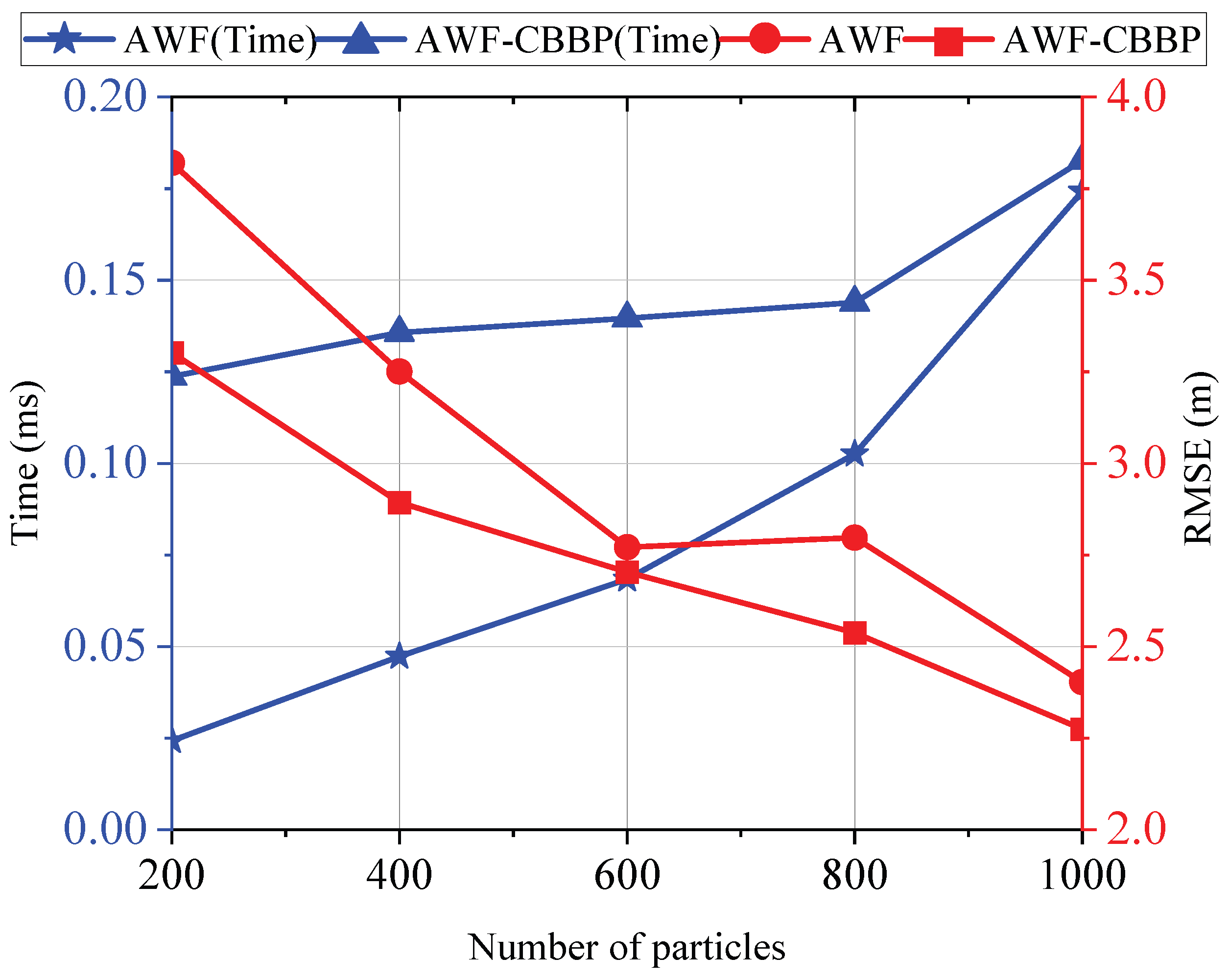
Then, to explore the influence of adding the self-recovery strategy on the execution time of the algorithm, experiments were conducted with different particle numbers to compare the resampling execution time with or without the self-recovery strategy. Figure 12 displays the trend of the algorithm resampling time and localization accuracy as the number of particles changed. It can be seen that as the number of particles increased, the resampling time continued to increase, and the positioning accuracy continued to improve. When the number of particles was small, compared with the conventional resampling algorithm, the self-recovery algorithm designed in this paper consumed more time. This is because the particle impoverishment problem is more likely to occur when the number of particles is small and the number of activations of the self-recovery algorithm is greater. As the number of particles increases, the frequency of particle impoverishment decreases, and the execution time of the self-recovery algorithm and conventional resampling algorithm draw gradually closer to each other. In terms of positioning accuracy, the self-recovery strategy designed in this paper can make the algorithm achieve the same accuracy under the condition of fewer particles, which shows good application potential in the real-time flight of a UAV swarm.

6. Conclusions

In this paper, we propose an adaptive Wasserstein filter (AWF) with distance-constrained bare bones self-recovery particles (CBBP) for a UAV swarm. Based on the particle filter algorithm, a transition particle-initialization strategy was designed, to suppress the cumulative error of the INS. The likelihood function was optimized, based on the sliced Wasserstein distance, which effectively quantifies the difference between the observed and prior data and has good robustness against distance-measurement noise under the strongly nonlinear model. In addition, to solve the problem of particle poverty, a diversity threshold based on particle purity was established, and a bare bones particle update rule with distance constraint was designed, to ensure the quality of the particles, thereby ensuring the accuracy of the algorithm. Through horizontal comparison simulation and a vertical ablation experiment, the availability and advantages of the algorithm were fully verified.