Abstract
Path planning is one of the most essential parts of autonomous navigation. Most existing works are based on the strategy of adjusting angles for planning. However, drones are susceptible to collisions in environments with densely distributed and high-speed obstacles, which poses a serious threat to flight safety. To handle this challenge, we propose a new method based on Multiple Strategies for Avoiding Obstacles with High Speed and High Density (MSAO2H). Firstly, we propose to extend the obstacle avoidance decisions of drones into angle adjustment, speed adjustment, and obstacle clearance. Hybrid action space is adopted to model each decision. Secondly, the state space of the obstacle environment is constructed to provide effective features for learning decision parameters. The instant reward and the ultimate reward are designed to balance the learning efficiency of decision parameters and the ability to explore optimal solutions. Finally, we innovatively introduced the interferometric fluid dynamics system into the parameterized deep Q-network to guide the learning of angle parameters. Compared with other algorithms, the proposed model has high success rates and generates high-quality planned paths. It can meet the requirements for autonomously planning high-quality paths in densely dynamic obstacle environments.
1. Introduction
As a critical technology reflecting the autonomous control capability of drones, the essence of path planning is to design a collision-free optimal path in the three-dimensional space environment from the starting position to the destination [1]. With the continuous development of air combat information technology, the airspace environment of drones is becoming increasingly complex. This complexity is reflected in the dense distribution of and dynamic changes in obstacles. The complex airspace environment presents significant challenges to the safety of drone flights. It is crucial to achieve autonomous obstacle-avoidance decision-making for drones to enhance the intelligent decision-making capabilities of control systems.
At present, in the field of path planning research, scholars from various countries are concentrating on improving the efficiency, completeness, and optimality of search paths. The achievements made are mainly divided into graph search algorithms [2,3,4,5,6,7], fluid/potential field algorithms [8,9,10,11,12,13,14], heuristic algorithms [15,16,17,18,19], and artificial intelligence learning algorithms. Graph search is the most effective search method for finding the shortest path in the static road network. Reference [5] used the Dijkstra algorithm to implement real-time path planning by defining the interest points of obstacles. However, path planning cannot be efficiently performed for dynamic obstacles. Fluid/potential field algorithms can generate a smooth virtual field based on the position of a target and the distribution of obstacles. The algorithms offer clear advantages in the smooth control of path planning and are widely utilized. Reference [11] introduced virtual sub-targets into an artificial potential field to achieve reasonable obstacle avoidance in complex environments. However, the algorithm lacks global information, making it only suitable for obstacle avoidance in local space. Reference [17] proposed a sand cat algorithm with learning behavior, which enables the UAV to plan a safe and feasible path at low cost. However, heuristic algorithms are typically suitable for simple or small environments. Their search efficiency decreases when the planning environment is complex, making it easy to become trapped in local optimal solutions. Observing that the path planning problem is a sequential decision-making problem, researchers turn to reinforcement learning (RL)-based methods [20,21,22]. Reference [22] built a maneuvering decision model using Q-learning and realized independent path planning in simulation environments. By integrating deep learning technology with reinforcement learning, deep reinforcement learning (DRL) [23,24,25,26,27,28,29,30,31] can acquire knowledge from the interaction between agents and the environment using neural networks. This approach is more closely aligned with the essence of biologic learning and can cope with complex and dynamic airspace environments. In addition, based on the nonlinear learning ability of neural networks, DRL can effectively extract useful features from high-dimensional data, such as continuous historical trajectory information of obstacles and the attributes of obstacles affecting the effectiveness of path planning. Reference [26] achieved autonomous navigation of drones in a multi-obstacle environment based on the twin delayed deep deterministic policy gradient (TD3) network. Reference [27] proposed the construction of sparse rewards to achieve automatic obstacle avoidance for drones based on the asynchronous advantage actor–critic (A3C) network. Reference [28] utilized the Q function of enhanced dueling double deep Q-networks (D3QN) with priority to implement UAV path planning in dynamic scenarios.
However, in the above research, the path planning environment is relatively simple. When the airspace environment of the drone is extremely complex, such as conducting reconnaissance, interpenetration, and other tasks in air combat, the obstacles may include vehicle-mounted phased array radar, anti-aircraft guns, electronic warfare aircraft, and other aircraft with striking capability. These obstacles are characterized by a highly dense distribution and high-speed dynamics. In such complex dynamic environments, it is challenging to plan safe routes effectively by relying solely on the decision of angle adjustment to avoid obstacles. Therefore, this paper aims to enhance the obstacle-avoidance decision-making of drones in complex airspace environments. This is achieved by adjusting the flight speed or direction or removing obstacles that significantly impact the quality of path planning in order to improve autonomous route planning capabilities.
Compared to discrete action spaces or continuous action spaces, hybrid action spaces can better describe complex problems by combining decision variables from multiple dimensions. This flexibility makes hybrid action spaces have more practical significance. In response to the diverse obstacle-avoidance decisions and their unique descriptive parameters, the hybrid action space can more effectively describe this situation, providing a research foundation. In addition, some scholars have developed deep reinforcement learning networks for hybrid action learning [32,33], which have been widely used in various decision-making problems such as games [34,35] and resource management [36,37].
Therefore, taking deep reinforcement learning as the core technical approach and analyzing the motion rules of drones, this paper proposes the Multiple Strategies for Avoiding Obstacles with High Speed and High Density (MSAO2H) model inspired by hybrid action space. The model aims to meet the requirements of autonomy and high quality in path planning for drones. The main contributions of this paper are:
(1) We propose three types of obstacle-avoidance decisions for drones. This is the first study on obstacle avoidance using three decisions: adjusting angles, adjusting speed, and obstacle clearance. Based on the hybrid action space, discrete obstacle-avoidance decisions and continuous action parameters are combined to improve the efficiency of path planning.
(2) In order to improve the learning efficiency of angle parameters, the interfered fluid dynamical system (IFDS) is innovatively introduced in the training process of the parametric deep Q network (PDQN). The model combines the advantages of PDQN in autonomous learning and IFDS in generating high-quality paths in complex dynamic obstacle environments, thereby enhancing the quality of path planning.
(3) Random environments with densely distributed and high-speed obstacles are designed in the GYM platform. The neural network is used to explore the interaction law between the drone and obstacle environments. The validity of the proposed method is verified in the scenarios.
The remainder of this paper is organized as follows. Section 2 briefly introduces the problem of path planning for drones. Section 3 introduces the relevant theories. Section 4 introduces the proposed method. Section 5 shows the simulation experiments and discussion. Section 6 presents the conclusions of this study.
2. Description of the Obstacle Environments
The complexity of the airspace environment is mainly reflected in the dense distribution of and dynamic changes in obstacles. Therefore, the obstacles in airspace are equivalent to moving spheres with a large radius in this paper, as shown in Equation (1) [38]:
where represents the position of the drone, represents the center point coordinates of the obstacle, and represents the radius of the obstacle.
In addition, we simulated the trajectories of obstacles through four different motion modes: static obstacles (Model 0), uniform linear motion (Model 1), horizontal uniform circular motion (Model 2), and serpentine motion (Model 3), whose motion laws are illustrated in Figure 1.

Figure 1.
Obstacle-avoidance decision space. (a) Model 1; (b) Model 2; (c) Model 3.
Based on the characteristics of obstacles, the blue dot in Figure 2 represents the starting point of the drone, which is fixed at [0, 0, 10,000]. The magenta dot represents the goal point of the drone, which is fixed at [10,000, 10,000, 20,000]. The initial positions of multiple obstacles are randomly simulated in the airspace range of km3. The number of obstacles is . We introduced noise to simulate the motion uncertainty of obstacles, making the simulated obstacles closer to those in the real world.
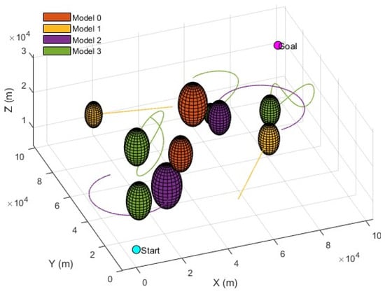
Figure 2.
Schematic diagram of dynamic obstacle environment.
In addition, the quality of path planning needs to be evaluated from the aspects of path length , tortuosity , and relative distance to the nearest obstacle . When is smaller, is smaller, and is farther, the comprehensive quality of the planned path is better, enabling it to better fulfill the high-quality planning requirements for paths in complex obstacle environments. The corresponding calculation formulas are as follows:
where is the position of the i-th obstacle, is the corresponding influence radius, and is the position of the n-th route node.
This research focuses on how one can autonomously plan high-quality paths in response to the large number of obstacles in the airspace and the dynamic changes in their positions.
3. Related Theories
3.1. PDQN
The PDQN is a kind of value-based reinforcement learning [39], which provides a general framework for effectively solving hybrid action space problems. As shown in Figure 3, the hybrid action space is represented as a tuple , where discrete actions are selected from a finite set and each action has a set of real-valued continuous parameters [40].
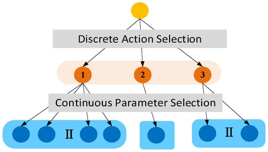
Figure 3.
Schematic diagram of hybrid action space structure.
The Bellman equation of the PDQN can be written as Equation (5):
where represent state space, rewards, and action respectively, and represents discount factor. Here, inside the conditional expectation on the right-hand side of Equation (5), they first solve Equation (6) for each :
Then, we select the largest . When the function Q is fixed, Equation (6) can be seen as the function . Then, the Bellman equation can be written as:
The value network is used to approximate , and the strategy network is used to approximate . are the parameters of the value network and the policy network, respectively. The loss functions are as shown in Equation (8), where is the loss function.
Based on the nonlinear mapping ability of PDQN, it can extract more meaningful features from the original input, helping the agent learn the hybrid action parameters better.
3.2. IFDS
The path planning method based on the IFDS simulates the macroscopic characteristics of water flow [41]. This method makes the generated path have the advantage of being smoother.
(1) Build the initial flow field model. Since the initial flow field model is not set to be affected by obstacles, the expression of the initial fluid vector velocity is as follows:
where represents the Euclidean distance between the point and the target point.
(2) Build the disturbed flow field model. The obstacles can cause disturbance to the initial flow field, and the impact expression is as follows:
is the unit attraction matrix, and the second and third terms are the repulsion matrix and the tangential matrix, respectively. is the tangential matrix. is a radial normal vector: .
(3) Calculate the confluent flow field and obtain the next point . In this way, a series of scattered points are obtained through iterative solutions and connected to form an interfered streamline, that is, the planned path.
determine the shape and direction of the planned path. The larger or is, the more drastically and earlier the agent avoids the obstacles.
4. Method
The MSAO2H model mainly consists of four components: the obstacle avoidance strategy space, the state space of obstacle environments, the reward of obstacle avoidance actions, and the training of the PDQN-IFDS.
4.1. Construction of the Multiple Obstacle-Avoidance Decision Space for Drones
According to the characteristics of obstacle environments and the needs of path planning described in Section 2, the obstacle-avoidance actions of drones include adjusting angles, adjusting speed, and obstacle clearance in this paper.
As shown in Figure 4a, the obstacle can be avoided by accelerating without changing the flight angles. In Figure 4b, the obstacle R1 has a larger influence range. After removing R1, the obstacle environment is greatly simplified. Therefore, the quality of path planning can be improved by adjusting the speed of drones or clearing obstacles to avoid dynamic obstacles. The specific analysis is as follows:
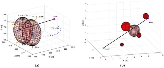
Figure 4.
Obstacle-avoidance decision space: (a) adjusting speed and (b) clearing obstacle R1.
(1) Adjusting angles: Considering the angular rate constraints of the climb angle and heading angle, the climb angle and heading angle at the next moment are adjusted as and , respectively:
where , are the change rates of the climb angle and heading angle at the next moment, and and are the maximum angular rates of the climb angle and heading angle.
(2) Adjusting speed: When the parameter of the adjusting speed is obtained, the flight speed of the drone at the next moment is . Considering the speed limit of drones, the speed is corrected according to Equation (12):
(3) Clearing obstacles: When remove = 0, this indicates that the clearing operation is not performed, and the drone interacts with the obstacle environment according to the original motion law. When remove = 1, the drone clears the obstacle, the number of obstacles decreases, and the maximum residual cost of the drone changes to . At the next moment, the drone obtains a new state space by interacting with the remaining obstacles. The initial remaining cost of obstacle clearance for the drone is 0.9.
Based on the above steps, the formula for calculating the position of the drone at the next moment is as follows:
4.2. Construction of the State Space
In order to improve the learning efficiency of the clearing parameter in specific situations, the descriptive factors , , and of obstacle attributes are constructed. The indicators are described as follows:
represents the cost of the drone to clear the obstacle, which is mainly determined by the vulnerability of obstacles. The greater the vulnerability of obstacles, the more difficult they are for the drone to clear, resulting in higher costs. In this paper, is set as [0.1,0.9].
represents the success rate of obstacle clearance, which is mainly affected by the speed of obstacles and the speed of the drone. When the obstacle is static, the success rate of clearance is the highest. When the speed of a dynamic obstacle is greater, the success rate of clearance is lower. Therefore, the calculation formula of is shown in Equation (14):
represents the benefits brought by removing obstacles for path planning, and the calculation is shown in Equation (15). The former term represents the obstruction degree of the obstacle, and the latter term represents the dispersion of the obstacle. are the corresponding weights.
The obstruction degree of the obstacle constructed is determined by the radius of the obstacle and the maximum influence radius of obstacles. As shown in Figure 5a, the larger the impact range of an obstacle, the more valuable it is for path planning. Equation (16) is constructed to describe the degree of dispersion between the obstacle and other obstacles. The denser the distribution of obstacles in the environment, the lower the benefits of removing obstacles. As shown in Figure 5b, the distribution of is relatively sparse. It is considered that clearing is more effective in improving the quality of path planning than clearing .
where is the line segment equation between the current obstacle and the flight endpoint, represents the distance from obstacle j to the line, and represents the number of obstacles that are close to the current obstacle () and closer to the flight endpoint than the current obstacle.

Figure 5.
Benefits of obstacle clearance: (a) the influence of obstacle radius and (b) the influence of obstacles distribution.
Based on the above analysis, state observations are obtained based on the interaction between the drone and obstacle environments and are defined as follows:
where are the relative positions of the drone and the nearest obstacle; are the relative positions of the nearest obstacle to the end point; are the relative velocity amplitude of the drone and the nearest obstacle; are respectively the heading angle and climb angle of the drone, represents the remaining cost of obstacle clearing for the drone, are the relative positions of the nearby obstacle j and the drone, and represents the position information of obstacle i at seven historical moments.
4.3. Construction of a Comprehensive Reward Mechanism
In order to improve the learning efficiency of action strategies and the exploration ability of global optimal solutions, a comprehensive reward mechanism was constructed, which includes dense instant reward and sparse ultimate reward.
4.3.1. The Instant Reward
The instant reward is reflected in the state of the drone, so it can provide immediate feedback to guide the agent to carry out the optimal action at each time step. The calculation formula is shown in Equation (18), including , , and . The specific analysis is as follows:
(1) Flight tendency reward : This represents the distance from the next point planned by the drone to the destination. A longer distance indicates that the drone has a trend of gradually approaching the destination, resulting in a shorter path length and a greater reward value.
(2) Flight safety reward : This is determined by the distance between the drone and the surface of the obstacle. The farther the distance from the obstacle, the longer the path length will inevitably be. Therefore, the flight safety threshold was set. When the distance from the obstacle surface is less than , the corresponding punishment will be given. is calculated as follows:
where , and is the distance between the drone and the center of the obstacle.
(3) Border security reward : In order to avoid the problem of the drone being unable to effectively learn parameters by adjusting its flight height to too high or too low, it is necessary to set boundary safety thresholds and , and impose the corresponding punishment when the flying altitude is low or high. The calculation formula is as follows:
4.3.2. The Ultimate Reward
At the end of the episode, the instant reward is disabled, and the ultimate reward is returned based on the status of the planning result to help the agent plan and make decisions for long-term goals. The final state is divided into four situations:
Situation 1: When the drone successfully reaches the end, it receives a reward for completing the planned mission. The calculation of the reward is shown in Equations (22) and (23).
where is the total length of the path. is the average flight speed. and represent the variation in flight angles within an adjacent sampling interval.
In addition, when the drone performs an obstacle-clearing action, the corresponding additional action reward is given. The reward calculation formula is as follows, where represents the number of obstacles cleared.
Situation 2: When the drone hits an obstacle, the episode ends and the drone receives a punishment. In order to improve the search ability of the action s, the punishment is set to be related to the position of the drone at the moment , as shown in Equation (25).
Situation 3: When the of the drone is less than 0, this indicates that the drone has carried out too many clearing obstacle operations. The learning of this episode is over, and the drone receives the corresponding punishment. The calculation method of punishment is similar to Equation (25).
Situation 4: When the drone flies out of the airspace, the corresponding punishment is obtained, and the calculation method of punishment is similar to Equation (25).
and are the final reward coefficients, and they are set to , where is the maximum time step. The reason for this is to avoid the drone focusing too much on instant rewards and ignoring the long-term path planning goal.
4.4. Learning of Obstacle-Avoidance Strategies Based on the PDQN-IFDS
4.4.1. The Structure of the PDQN-IFDS
The angle adjustment of the drone involves learning two continuous parameters: climbing angle and heading angle. It is necessary to find the optimal combination of continuous parameters, which causes the problem of difficult convergence of the algorithm and poor path planning quality. When the IFDS is introduced, the parameters of angles become , , and . The three parameters are closely related to the position of the drone and the position and radius of obstacles, and they determine the direction, shape, and avoidance time of path planning.
The PDQN is used to train the probability distribution of parameters to guide the learning of climb angle and heading angle, as shown in Equation (26), so as to effectively improve the learning efficiency of obstacle-avoidance strategies.
The PDQN-IFDS is divided into four neural networks, namely ParamActorNet, Q-Net, ParamActor-TargetNet, and Q-TargetNet. The structure of ParamActorNet is divided into four layers, with network nodes of 40, 128, 256, and 5, respectively. The 40 nodes of the input layer correspond to the size of the state space (Equation (17)). The number of output nodes corresponds to the 5 parameters of the hybrid action space. ,,, , and remove is 0/1. Each parameter is normalized to [−1,1], which avoids the problems of inconsistent convergence speed and gradient instability. The structure of Q-net is still divided into four layers, and the corresponding network nodes are 45, 128, 256, and 3. The number of output nodes corresponds to three different obstacle-avoidance decisions: adjusting angles, adjusting speed, and obstacle clearance. ParamActor-TargetNet and Q-TargetNet are obtained by copying parameters from ParamActorNet and Q-Net.
4.4.2. The Training Process of the PDQN-IFDS
Based on the loss function of the PDQN-IFDS in Section 3.1, the gradient of on the Q-Net network parameter can be expressed as Equation (27), and is updated via the gradient descent method: , where is the learning rate.
ParamActorNet is designed to maximize the cumulative expected return, and is updated by policy gradients: .
The soft update is adopted for ParamActor-TargetNet and Q-TargetNet, as shown in Equation (29).
4.5. MSAO2H Model
We designed the random obstacle environments in the development framework of OpenAI Gym 0.10.5. According to the introduction in Section 4.1, Section 4.2, Section 4.3, Section 4.4, the interaction process of the four parts is shown in Figure 6: By inputting the real-time status of the drone and the obstacle environment (Section 4.1) into the PDQN-IFDS (Section 4.4), the drone learns the best obstacle avoidance strategies (Section 4.2) under the guidance of the reward mechanism (Section 4.3), so as to complete a sequential decision process of path planning.
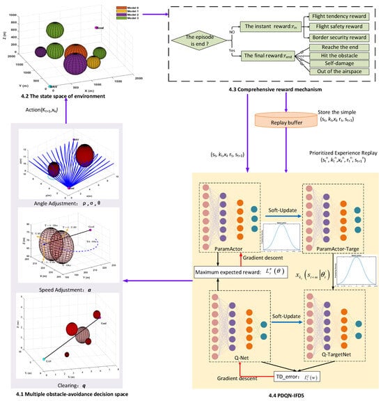
Figure 6.
Flow chart of the autonomous path planning algorithm of drones based on MSAO2H.
The MSAO2H model training process is shown in Algorithm 1:
| Algorithm 1: The training process of MSAO2H |
| Initialization: Randomly initialize ,, targrt nets ; Replay memory D; |
| for episode ⬅ 1 to Max do |
| for step t ⬅ 1 to TMax or do |
| Obtain initial state: S (by Equations (14)–(17)); |
| Execute the action (by Equations (11)–(13) and (26)); |
| Obtain reward r and new state St+1 (by Equations (18)–(25)); |
| Update step counters: t ⬅ t + 1; |
| Store the simple in D; |
| Obtain random a batch of from D; |
| Update ParamActorNet, Q-Net, ParamActor-TargetNet, Q-TargetNet (by Equations (27)–(29)). end for |
| end for |
5. Simulation Experiment and Analysis
We designed obstacle environments in the OpenAI Gym 0.10.5 development framework for autonomous path planning of the drone. Through the interaction between the drone and the obstacles, data were collected. As a random environment, at the episode end of obstacle avoidance tasks, obstacles in the airspace will be reinitialized randomly. Considering the motion constraints of the drone, the climbing angle of the drone was set to and the speed was set to . The time step was 20 s, and the maximum changes in the heading angle and climb angle of the drone at each step were 15° and 8°, respectively. This paper analyzes the impact of the proposed method on path planning from two perspectives:
(1) In the random training environments, the average success rate and average reward of the deep deterministic policy gradient (DDPG), DDPG-IFDS, PDQN, and MSAO2H are compared to verify the effectiveness of the diversified obstacle-avoidance decisions.
(2) We compared the results based on different methods in test environments to verify the versatility of MSAO2H.
5.1. Analysis of Effectiveness
The training convergence results of the DDPG, DDPG-IFDS, PDQN, and MSAO2H during training were compared. The DDPG and DDPG-IFDS only adjust the climbing angle and heading angle of the drone for route planning. PDQN and MSAO2H perform route planning by making three types of obstacle-avoidance decisions: adjusting angles, adjusting speed, and clearing obstacles. The DDPG-IFDS and MSAO2H learn the parameters of angle adjustment based on the IFDS algorithm. In the training process, the -greedy algorithm [39] was adopted, with the initial value ε of 0.9, gradually decreasing to 0.01 as the number of iterations increases. The parameters of the PDQN are shown in Table 1.

Table 1.
Parameter settings of the PDQN.
The number of training iterations was set to 4 million times, and the average reward and average success rate were calculated every 1000 iterations. The training convergence results of the four models are shown in Figure 7.
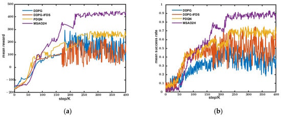
Figure 7.
The convergence iteration results based on different networks: (a) the convergence of average reward and (b) the convergence of average success rate.
Due to there being fewer parameters of obstacle avoidance action in the DDPG and DDPG-IFDS, they exhibit faster convergence speeds compared to the algorithms based on hybrid action space. However, the convergence average reward and convergence average success rate are lower. Additionally, the average reward value and average success rate fluctuate greatly, indicating that these two models are highly sensitive to obstacle environments and difficult to apply widely. The average reward during the initial stage of PDQN training (0–100 K iterations) increases more rapidly than that of MSAO2H. But the PDQN shows a slower increase in rewards during the later stages. After 260 K iterations of training, the PDQN gradually converged. The average reward and average success rate after convergence are lower than those of MSAO2H. This suggests that the avoidance decisions learned from the PDQN have certain limitations. Although the average reward and average success rate of MSAO2H are low in the initial learning stage, after 220K iterations, the average reward converges to a high value, and the average success rate converges to 0.92. The main reason for the phenomenon is that the model transforms challenging-to-learn parameters into parameters related to the relative position and radius of the nearest obstacle. This physical interpretation can help to comprehend angle adjustments and improve the learning efficiency of obstacle-avoidance actions.
The training results, based on the random obstacle environments, show that the proposed method can effectively complete the avoidance tasks, and the proposed model demonstrates a certain level of generalization.
5.2. Analysis of Versatility
5.2.1. Analysis of Planning Results in Simple Obstacle Environments
We compared the path planning results based on Astar, the IFDS, rapidly-exploring random tree (RRT), DDPG, DDPG-IFDS, PDQN, and MSAO2H in the airspace of 12 static obstacles, as shown in Figure 8.
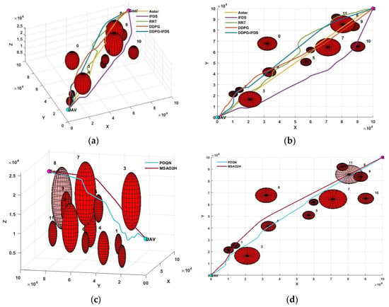
Figure 8.
Result of path planning in a simple environment: (a) The three-dimensional paths based on Astar, the IFDS, RRT, DDPG, and DDPG-IFDS; (b) the two-dimensional results based on Astar, the IFDS, RRT, DDPG, and DDPG-IFDS; (c) the three-dimensional paths based on the PDQN and MSAO2H; (d) the two-dimensional results based on the PDQN and MSAO2H.
The angles of the drone and their variation are shown in Figure 9. The trend of the distance from the nearest obstacle during flight is shown in Figure 10. Table 2 shows the , , and of the paths obtained by seven algorithms.
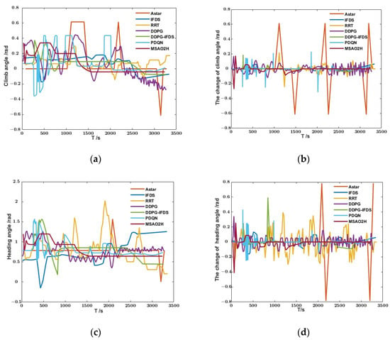
Figure 9.
The change in the flight angle of the drone: (a) the climb angle of the drone; (b) the climb change rate of the drone; (c) the heading angle of the drone; (d) the heading change rate of the drone.
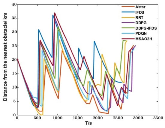
Figure 10.
The variation in the distance of the drone to the nearest obstacle.

Table 2.
Evaluation results of planning paths in a simple environment.
Compared with Figure 9 and Figure 10, it can be observed from the path planning results based on Astar that the climb angle of the drone and its variation amplitude exceed the constraint conditions, resulting in low path smoothness and falling into the local optimal solution. Due to the random sampling and exploration method of the RRT, the climbing angle and heading angle fluctuate significantly, leading to a longer planned path length. Furthermore, the closest distance to the obstacle surface is 93 m, indicating a low level of path safety and poor overall path planning quality. Compared to the RRT and Astar, the path planning results based on the IFDS show a safe distance from obstacles, as well as more gradual changes in climb angle and heading angle. The resulting path is smoother, but the quality of the path depends on the hyperparameter settings. The planning result is based on the IFDS with , , and .
By using deep reinforcement learning to learn the distribution of hyperparameters in the IFDS, it is possible to dynamically adjust parameters for various obstacles and improve adaptive capabilities. As shown in Table 2, the path planned by the DDPG-IFDS exhibits similar tortuosity compared to the IFDS model. It maintains a longer distance from the obstacle surface (the nearest distance is 1400 m) while reducing the length of the path planning result by 2.81%. The length and tortuosity of the path based on MSAO2H were reduced by 3.03% and 10.62%, respectively.
In the planning results based on hybrid action networks (PDQN and MSAO2H), obstacle 8 is cleared. According to Table 2, it can be seen that the planned path is significantly shortened compared to the DDPG and DDPG-IFDS. Therefore, the obstacle clearance decision represents a more optimal solution. Although the PDQN and DDPG reduce the path length to a certain extent, it can be seen from Figure 10 that both of them have the problem of significant fluctuations in the climb angle, resulting in poor path smoothness.
As shown in Table 2, the path generated by MSAO2H has the shortest length, the lowest degree of tortuosity, and a safe distance from the nearest obstacle, resulting in higher comprehensive path planning quality. The results indicate that the proposed model achieves excellent performance.
5.2.2. Analysis of Planning Results in a Complex Obstacle Environment
Due to the lack of sensitivity to the perception of dynamic environments for traditional algorithms, it is difficult to respond promptly to the dynamic obstacles. In this paper, we compare the path planning results based on deep reinforcement network models in a dynamic obstacle environment. There are 21 obstacles in the simulated dynamic environment. Of them, 5 obstacles are static obstacles, 6 obstacles are in linear motion, 4 obstacles are in horizontal circular motion, and 6 obstacles are in serpentine motion. In this environment, the path planning results based on the DDPG, DDPG-IFDS, PDQN, and MSAO2H models are shown in Figure 11, Figure 12, Figure 13 and Figure 14, respectively. To enhance the presentation of path planning results in the dynamic obstacle environment, only the time when each obstacle is closest to the drone, the corresponding position, and the path information of the closest obstacle in a short time are exclusively highlighted in Figure 11, Figure 12, Figure 13 and Figure 14. The change in the relative distance to the nearest obstacle during flight is shown in Figure 15. Similarly, , , and of the paths are shown in Table 3.
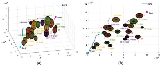
Figure 11.
Result of path planning based on the DDPG in a complex environment: (a) three-dimensional path and (b) X-Y plane projection.
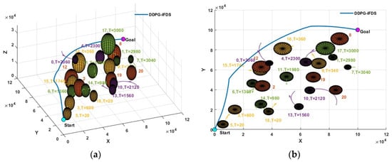
Figure 12.
Result of path planning based on the DDPG-IFDS in a complex environment: (a) three-dimensional path and (b) X-Y plane projection.
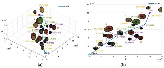
Figure 13.
Result of path planning based on the PDQN in a complex environment: (a) three-dimensional path and (b) X-Y plane projection.
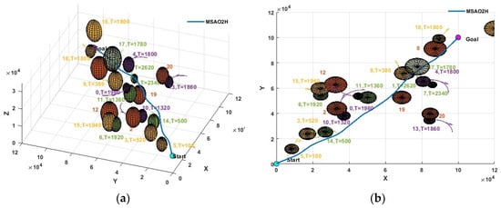
Figure 14.
Result of path planning based on MSAO2H in a complex environment: (a) three-dimensional path and (b) X-Y plane projection.
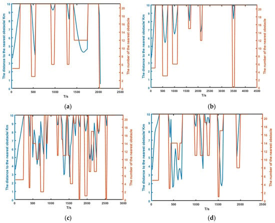
Figure 15.
Distance to the nearest obstacle during flight; (a) based on the DDPG; (b) based on the DDPG-IFDS; (c) based on the PDQN; (d) based on MSAO2H.

Table 3.
Evaluation results of planning paths in a complex dynamic environment.
As shown in Figure 11, the DDPG model failed to avoid obstacle 0. In contrast, the paths of the other three models were successfully planned. The results in Figure 13 and Figure 14 show that th ePDQN and MSAO2H can successfully plan a safe route in areas with a dense obstacle distribution based on three obstacle avoidance decisions. The difference is that PDQN clears obstacles 3 and 17, while MSAO2H only clears obstacle 17, and the clearing cost based on MSAO2H is lower.
In addition, we analyzed the changes in the relative distance between the drone and the nearest obstacle during flight, as shown in Figure 15. The horizontal axis represents the flight time of the drone. The blue line on the left vertical axis represents the relative distance between the drone and the nearest obstacle. The red line on the right vertical axis represents the number of the nearest obstacle (0–20 represents the number of the 21 obstacles; 21 means no obstruction within 10 km).
According to Figure 15a, the DDPG fails to avoid obstacle 0 at resulting in the failure of path planning. It can be seen from Figure 15b that the distance between the drone and obstacles is relatively far on the whole. According to Figure 12, the main reason for the phenomenon is that the DDPG-IFDS is planned in areas with a relatively wide distribution of obstacles, which causes the path length to be too large (the length is 165,946 m). The number of the nearest obstacle changes rapidly as shown in Figure 15c,d, indicating that the PDQN and MSAO2H can be applied to complex obstacle environments with high dynamics. Compared with Figure 15c, the change in the number of nearest obstacles is slower and the average distance from the nearest obstacle is longer in Figure 15d. This suggests that the path planned based on the MSAO2H model is more secure.
As shown in Table 3, compared with the results of path planning under the obstacle environment in Section 5.2.1, the path length increases and the smoothness decreases in the dynamic environment. However, the path planned based on MSAO2H still has the shortest length and the highest smoothness and maintains a certain safety range with obstacles, resulting in the highest quality of planned paths. The length and tortuosity of the path obtained by MSAO2H are 1.62% and 10.55% lower than those obtained by the PDQN, respectively. This result indicates that the obstacle-avoidance decisions learned by MSAO2H are more effective.
5.2.3. Analysis of Planning Results in Random Obstacle Environments
To further verify the versatility of MSAO2H, the performance of four models in 200 randomly generated obstacle environments was compared. We took 10 environments as a test set and calculated the average reward and average success rate of different models in each test set, as shown in Figure 16:
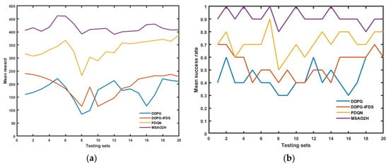
Figure 16.
Test results of path planning in random obstacle environments: (a) the average reward and (b) the average success rate.
Based on Figure 16, it is evident that the DDPG achieves its highest average reward of 221 in the fifth test set. The DDPG-IFDS surpasses this, attaining the highest average reward of 240 in the first test set. The PDQN outperforms both with a maximum average reward of 368 in the sixth test set. However, MSAO2H exhibits the most significant performance, securing the highest average reward of 461 in the fifth test set. The four models exhibit lower reward values in the eighth test set, with values of 84, 114, 232, and 392, respectively. Compared to the other models, MSAO2H demonstrates the smallest fluctuation in average reward in random testing environments. Additionally, the DDPG, DDPG-IFDS, and PDQN achieve their maximum success rates of 0.6, 0.7, and 0.9, respectively, in the test sets. Meanwhile, MSAO2H achieves the path success rate of one in five test sets, with a minimum success rate of 0.8 in the eighth set.
In 200 test environments, the average reward values of the four models are 173.19, 194.76, 335.09, and 415.456, and the average success rates are 0.45, 0.54, 0.715, and 0.915, respectively. These results indicate that MSAO2H has a higher average reward and success rate in the test environments, confirming the higher robustness of MSAO2H to the environment.
6. Conclusions
By constructing the state space of obstacle environments, various obstacle-avoidance strategies, a comprehensive reward mechanism, and the PDQN-IFDS, the MSAO2H model was constructed to achieve autonomous path planning for drones in dynamic and complex airspace environments. And compared with other methods, the effectiveness of the proposed method was verified:
(1) MSAO2H can continuously optimize the obstacle-avoidance decisions of drones based on feedback information from random dynamic obstacle environments. The average success rate of convergence and the average reward of convergence are high, which improves the autonomous capability of path planning and validates the generalization of the model.
(2) Compared to traditional path planning algorithms such as Astar, RRT, and IFDS, the proposed method has shorter and less tortuous degree planning results in the static obstacle environment while maintaining a safe distance from obstacle surfaces. The results have validated the fact that multiple obstacle avoidance decisions can effectively improve the quality of path planning.
(3) Compared with the DDPG and DDPG-IFDS, the proposed method can successfully plan routes in areas with dense obstacles. Compared with the PDQN, MSAO2H can converge more quickly and stably and plan high-quality paths. The results show that the proposed model makes path planning for drones in complex dynamic obstacle environments more reliable and efficient.
In this paper, deep reinforcement learning was used to study the global path planning method based on the motion constraints of drones. In the future, multi-agent reinforcement learning will be used to further study dynamic path planning under the constraints of autonomous navigation for formation and cluster cooperation.
Author Contributions
Conceptualization, F.Y.; methodology, T.Y. and D.L.; validation, T.Y.; formal analysis, T.Y., F.Y. and D.L.; data curation, T.Y. and D.L.; writing—original draft preparation, T.Y.; writing—Review and Editing, F.Y.; supervision, D.L.; funding acquisition, F.Y. All authors have read and agreed to the published version of the manuscript.
Funding
This research was funded by the Fundamental Research Program of Shanxi Province, grant No. 202203021221104, and the National Natural Science Foundation of China, grant No. 61972363.
Data Availability Statement
The data presented in this study are available from the corresponding author upon request.
Conflicts of Interest
The authors declare no conflicts of interest.
References
- Zhou, C.; Gu, S.; Wen, Y. The review unmanned surface vehicle path planning: Based on multi-modality constraint. Ocean. Eng. 2020, 200, 107043. [Google Scholar] [CrossRef]
- Wu, X.; Xu, L.; Zhen, R.; Wu, X. Bi-directional adaptive A*algorithm toward optimal path planning for large-scale UAV under multi-constraints. IEEE Access 2020, 8, 85431–85440. [Google Scholar] [CrossRef]
- Ren, Z.; Rathinam, S.; Choset, H. Multi-Objective Path-Based D* Lite. IEEE Robot. Autom. Lett. 2021, 7, 3318–3325. [Google Scholar] [CrossRef]
- Niu, H.; Savvaris, A.; Tsourdos, A.; Ji, Z. Voronoi-visibility roadmap-based path planning algorithm for unmanned surface vehicles. J. Navig. 2019, 72, 850–874. [Google Scholar] [CrossRef]
- Bashir, N.; Boudjit, S.; Dauphin, G.; Zeadally, S. An obstacle avoidance approach for UAV path planning. Simul. Model. Pract. Theory 2023, 129, 102815. [Google Scholar] [CrossRef]
- Xu, X.; Zhang, F.F.; Zhao, Y. Unmanned Aerial Vehicle Path-Planning Method Based on Improved P-RRT* Algorithm. Electronics 2023, 12, 4576. [Google Scholar] [CrossRef]
- Yuan, M.S.; Zhou, T.L.; Chen, M. Improved lazy theta* algorithm based on octree map for path planning of UAV. Def. Technol. 2023, 23, 8–18. [Google Scholar] [CrossRef]
- Wang, S.; Lin, F.; Wang, T.; Zhao, Y.; Zang, L.; Deng, Y. Autonomous Vehicle Path Planning Based on Driver Characteristics Identification and Improved Artificial Potential Field. Actuators 2022, 11, 52. [Google Scholar] [CrossRef]
- Celestini, D.; Primatesta, S.; Capello, E. Trajectory Planning for UAVs Based on Interfered Fluid Dynamical System and Bézier Curves. IEEE Robot. Autom. Lett. 2022, 7, 9620–9626. [Google Scholar] [CrossRef]
- Wu, J.; Wang, H.; Zhang, M. On obstacle avoidance path planning in unknown 3D environments: A fluid-based framework. ISA Trans. 2020, 111, 249–264. [Google Scholar] [CrossRef]
- Hao, G.Q.; Lv, Q.; Huang, Z.; Zhao, H.L.; Chen, W. UAV Path Planning Based on Improved Artificial Potential Field Method. Aerospace 2023, 10, 562. [Google Scholar] [CrossRef]
- Diao, Q.; Zhang, J.; Liu, M.; Yang, J. A Disaster Relief UAV Path Planning Based on APF-IRRT* Fusion Algorithm. Drones 2023, 7, 323. [Google Scholar] [CrossRef]
- Goricanec, J.; Milas, A.; Markovic, L.; Bogdan, S. Collision-Free Trajectory Following With Augmented Artificial Potential Field Using UAVs. IEEE Access 2023, 11, 83492–83506. [Google Scholar] [CrossRef]
- Hao, Z.; Xiong, H.L.; Liu, Y. Trajectory Planning Algorithm of UAV Based on System Positioning Accuracy Constraints. Electronics 2020, 9, 250. [Google Scholar] [CrossRef]
- Phung, M.D.; Hao, P. Safety-enhanced UAV path planning with spherical vector-based particle swarm optimization. Appl. Soft Comput. 2021, 2, 107376. [Google Scholar] [CrossRef]
- Miao, C.; Chen, G.; Yan, C. Path planning optimization of indoor mobile robot based on adaptive ant colony algorithm. Comput. Ind. Eng. 2021, 156, 107230. [Google Scholar] [CrossRef]
- Hu, K.; Mo, Y. A novel unmanned aerial vehicle path planning approach: Sand cat optimization algorithm incorporating learned behaviour. Meas. Sci. Technol. 2024, 35, 046203. [Google Scholar] [CrossRef]
- Zhou, X.J.; Tang, Z.H.; Wang, N.; Yang, C.H.; Huang, T.W. A novel state transition algorithm with adaptive fuzzy penalty for multi-constraint UAV path planning. Expert Syst. Appl. 2024, 248, 123481. [Google Scholar] [CrossRef]
- Wu, X.J.; Xu, L.; Zhen, R.; Wu, X.L. Global and Local Moth-flame Optimization Algorithm for UAV Formation Path Planning Under Multi-constraints. Int. J. Control. Autom. Syst. 2023, 21, 1032–1047. [Google Scholar] [CrossRef]
- Ji, M.; Zhang, L.; Wang, S. A Path Planning Approach Based on Q-learning for Robot Arm. In Proceedings of the 2019 3rd International Conference on Robotics and Automation Sciences (ICRAS), Wuhan, China, 1–3 June 2019. [Google Scholar]
- Chen, C.; Chen, X.Q.; Ma, F. A knowledge-free path planning approach for smart ships based on reinforcement learning. Ocean. Eng. 2019, 189, 106299. [Google Scholar] [CrossRef]
- Hao, B.; Du, H.; Yan, Z.P. A path planning approach for unmanned surface vehicles based on dynamic and fast Q-learning. Ocean. Eng. 2023, 270, 113632. [Google Scholar] [CrossRef]
- Qian, S.; Lam, H.K.; Xuan, C.B.; Chen, M. Adaptive neuro-fuzzy PID controller based on twin delayed deep deterministic policy gradient algorithm. Neurocomputing 2020, 402, 183–194. [Google Scholar]
- Tao, Y.; Zhang, W.A.; Simon, X.; Yang, L.Y. Soft Actor-Critic Reinforcement Learning for robotic manipulator with Hindsight Experience Replay. Int. J. Robot. Autom. 2019, 34, 536–543. [Google Scholar]
- Li, Y.; Zhang, S.; Ye, F. A UAV Path Planning Method Based on Deep Reinforcement Learning. In Proceedings of the 2020 IEEE USNC-CNC-URSI North American Radio Science Meeting (Joint with AP-S Symposium), Toronto, ON, Canada, 5–10 July 2020. [Google Scholar]
- Zhang, S.; Li, Y.; Dong, Q. Autonomous navigation of UAV in multi-obstacle environments based on a Deep Reinforcement Learning approach—ScienceDirect. Appl. Soft Comput. 2021, 115, 115. [Google Scholar]
- Wang, C.; Wang, J.; Wang, J. Deep Reinforcement Learning-based Autonomous UAV Navigation with Sparse Rewards. IEEE Internet Things J. 2020, 7, 6180–6190. [Google Scholar] [CrossRef]
- Tang, J.; Liang, Y.; Li, K. Dynamic Scene Path Planning of UAVs Based on Deep Reinforcement Learning. Drones 2024, 8, 60. [Google Scholar] [CrossRef]
- Yan, C.; Xiang, X.; Wang, C. Towards Real-Time Path Planning through Deep Reinforcement Learning for a UAV in Dynamic Environments. J. Intell. Robot Syst. 2020, 98, 297–309. [Google Scholar] [CrossRef]
- Zhou, Y.X.; Shu, J.S.; Hao, H.; Song, H.; Lai, X.C. UAV 3D online track planning based on improved SAC algorithm. J. Braz. Soc. Mech. Sci. Eng. 2023, 46, 12. [Google Scholar] [CrossRef]
- Luo, X.Q.; Wang, Q.Y.; Gong, H.F.; Tang, C. UAV Path Planning Based on the Average TD3 Algorithm With Prioritized Experience Replay. IEEE Access 2021, 12, 38017–38029. [Google Scholar] [CrossRef]
- Zhou, F.; Rui, S.; Zhang, W. Hybrid Actor-Critic Reinforcement Learning in Parameterized Action Space. arXiv 2019, arXiv:1903.01344. [Google Scholar] [CrossRef]
- Xu, Y.H.; Wei, Y.R.; Jiang, K.Y.; Chen, L.; Wang, D.; Deng, H.B. Action decoupled SAC reinforcement learning with discrete-continuous hybrid action spaces. Neurocomputing 2023, 537, 141–151. [Google Scholar] [CrossRef]
- Chen, S.Q.; Su, R. An autonomous agent for negotiation with multiple communication channels using parametrized deep Q-network. Math. Biosci. Eng. 2022, 19, 7933–7951. [Google Scholar] [CrossRef]
- Bester, C.J.; James, S.D.; Konidaris, G.D. Multi-Pass Q-Networks for Deep Reinforcement Learning with Parameterised Action Spaces. arXiv 2019, arXiv:1905.04388. [Google Scholar] [CrossRef]
- Huang, C.; Zhang, H.; Wang, L. Mixed Deep Reinforcement Learning Considering Discrete-continuous Hybrid Action Space for Smart Home Energy Management. J. Mod. Power Syst. Clean Energy 2022, 10, 743–754. [Google Scholar] [CrossRef]
- Ale, L.; King, S.A.; Zhang, N. D3PG: Dirichlet DDPG for Task Partitioning and Offloading with Constrained Hybrid Action Space in Mobile Edge Computing. IEEE Internet Things J. 2021, 9, 19260–19272. [Google Scholar] [CrossRef]
- Wu, J.; Wang, H.; Li, N. Formation Obstacle Avoidance: A Fluid-Based Solution. IEEE Syst. J. 2019, 14, 1479–1490. [Google Scholar] [CrossRef]
- Xiong, J.; Wang, Q.; Yang, Z. Parametrized Deep Q-Networks Learning: Reinforcement Learning with Discrete-Continuous Hybrid Action Space. arXiv 2018, arXiv:1810.06394. [Google Scholar] [CrossRef]
- Schulman, J.; Wolski, F.; Dhariwal, P.; Radford, A.; Klimov, O. Proximal policy optimization algorithms. arXiv 2017, arXiv:1707.06347. [Google Scholar] [CrossRef]
- Wu, J.F.; Wang, H.L.; Wang, Y.X. UAV Reactive Interfered Fluid Path Planning. Acta Autom. Sin. 2021, 47, 1–16. [Google Scholar]
Disclaimer/Publisher’s Note: The statements, opinions and data contained in all publications are solely those of the individual author(s) and contributor(s) and not of MDPI and/or the editor(s). MDPI and/or the editor(s) disclaim responsibility for any injury to people or property resulting from any ideas, methods, instructions or products referred to in the content. |
© 2024 by the authors. Licensee MDPI, Basel, Switzerland. This article is an open access article distributed under the terms and conditions of the Creative Commons Attribution (CC BY) license (https://creativecommons.org/licenses/by/4.0/).