Article

Model-Free RBF Neural Network Intelligent-PID Control Applying Adaptive Robust Term for Quadrotor System

1
The Industrial Science Technology Research Center, Pukyong National University, Busan 48513, Republic of Korea
2
Major of Mechanical System Engineering, Pukyong National University, Busan 48513, Republic of Korea
*
Author to whom correspondence should be addressed.
Drones 2024, 8(5), 179; https://doi.org/10.3390/drones8050179
Submission received: 28 March 2024 / Revised: 26 April 2024 / Accepted: 29 April 2024 / Published: 1 May 2024

Abstract

:
This paper proposes a quadrotor system control scheme using an intelligent–proportional–integral–differential control (I-PID)-based controller augmented with a radial basis neural network (RBF neural network) and the proposed adaptive robust term. The I-PID controller, similar to the widely utilized PID controller in quadrotor systems, demonstrates notable robustness. To enhance this robustness further, the time-delay estimation error was compensated with an RBF neural network. Additionally, an adaptive robust term was proposed to address the shortcomings of the neural network system, thereby constructing a more robust controller. This supplementary control input integrated an adaptation term to address significant signal changes and was amalgamated with a reverse saturation filter to remove unnecessary control input during a steady state. The adaptive law of the proposed controller was designed based on Lyapunov stability to satisfy control system stability. To verify the control system, simulations were conducted on a quadrotor system maneuvering along a spiral path in a disturbed environment. The simulation results demonstrate that the proposed controller achieves high tracking performance across all six axes. Therefore, the controller proposed in this paper can be configured similarly to the previous PID controller and shows satisfactory performance.

1. Introduction

Quadrotors have symmetric structures and high maneuverability, enabling hovering and demonstrating good flight performance. Currently, these characteristics find application across various industries, leveraging their capabilities [1,2,3]. Moreover, quadrotors are garnering significant attention not only for practical applications but also from researchers. Despite their favorable behavior, quadrotor systems present significant control challenges due to strong nonlinear coupling dynamics, model uncertainties, unmeasurable disturbances, and under-actuated problems. Consequently, these complexities pose formidable challenges for control engineers, prompting extensive research efforts [3,4,5,6,7,8,9,10,11,12,13,14,15,16,17].
In [7], dynamics were estimated using FCRNN (Fully Connected Recurrent Neural Network) and controlled using ISMC (Integral Sliding Mode Control). In [8], trajectory tracking was achieved by applying RGSMC (Rapid Global Sliding Mode Control) using a fast decay function. Attitude stabilization was attained in [13] through a nominal state-feedback controller and a robust compensator, while [14] utilized the PD2 feedback structure for the same purpose. Furthermore, Ref. [15] accomplished robust attitude control against disturbances through a switching model predictive attitude controller, showcasing promising results. Ref. [16] introduced a dynamic event-triggered control strategy that maximized the efficiency of maritime search operations through the collaboration of USVs and UAVs. The strategy enhanced system stability by efficiently managing key control inputs and robustly resisting external disturbances. Ref. [17] presented a control algorithm designed to efficiently perform path-following tasks through the cooperation of USVs and UAVs. Aiming to minimize complex design requirements and command transmissions, it utilizes a dynamic event-triggered mechanism to reduce data transmission and maximize system efficiency.
Their research shows excellent results. However, their control methods use model information. Since system identification of a control system is difficult, it can be hard to apply to a quadrotor system. Therefore, in one study, a quadrotor was controlled using a PID controller, a representative, model-free control method. It can be applied to various quadrotor systems with a simple control method and can lead to satisfactory performance. Although this control method has the advantage of being easy to apply, it also has the disadvantage of reducing control performance due to external forces and system uncertainty. Thus, this paper proposes a control method that combines an I-PID (Intelligent-PID) controller and an RBF (Radial Basis Function) neural network.
I-PID control is a model-free nonlinear control method [18,19,20], which offers advantages for application in complex systems such as robots and quadrotors. This method relies on previous control inputs and outputs rather than modeling information. Therefore, this method is one of the promising control techniques that can replace traditional PID, and there are currently results of its application to various types of plants [18,19,20]. Moreover, this controller exhibits similarities to time-delay estimation errors and a lack of robustness in the transient state [20,21,22]. In particular, time-delay estimation error is a problem that must be solved as it reduces the robustness of the controller and deteriorates control performance. To mitigate this issue, we employed an artificial neural network for compensation.
Artificial neural networks are powerful tools for solving control problems such as nonlinearity and disturbance approximation. In addition, a neural network does not require complex mathematical analysis such as disturbance observers and can be configured independently of the system [23,24,25,26]. These features can be implemented without the model information required in this paper and are easy to apply to the controller. However, neural networks have some disadvantages when online learning. Firstly, neural networks require a lot of computation. This can increase computation time and reduce the control rate. Secondly, neural networks are difficult to mathematically analyze. This issue combines with control systems to make stability analysis difficult. Thirdly, due to initial value problems, neural networks can make control systems unstable. This paper addresses this issue by employing an RBF neural network and an adaptive robust term for compensation.
The RBF neural network has a simple structure consisting of one layer each. The advantage of this neural network is that it is mathematically analyzed, and the computational amount is smaller than for other neural networks. Therefore, as in this paper, it is evaluated as a neural network suitable for mechatronics system control [27,28,29,30,31,32,33,34]. The activation function uses a Gaussian function. This function follows a probability distribution and has excellent nonlinear approximation ability when used with neural networks [27,28,29,30,31]. However, a challenge arises as Gaussian functions are not differentiable. In this paper, we design a Lyapunov-based update law to consider control system stability without using differentiation in the activation function.
To overcome some of the shortcomings of neural networks, we used adaptive robust terms. An adaptive robust term originates from a robust term. A robust term consists of constant gain and error sign functions. This ability of the robust term nicely suppresses the shortcomings that occur during the online learning of neural networks [29,30,31,32,33,34,35]. Although this may reduce the estimation performance of the network, it is a practical way to make control systems containing neural networks more robust. However, robust terms also have some disadvantages. A robust term uses constant control gain and cannot respond to large signal changes. Additionally, by generating unnecessary control inputs under a steady state, there is a risk of worsening control performance in a steady state and causing chattering. Therefore, we propose an adaptive robust term that can dynamically adapt to signal changes by adjusting the control gain and that utilizes a reverse saturation filter that can remove unnecessary control inputs in the steady state. In conclusion, this paper proposes I-PID control, which can be configured similarly to PID and is more robust to disturbances. This study used the RBF neural network to compensate for the time-delay estimation error, which is a drawback of I-PID. Afterwards, we proposed an adaptive robust term to overcome the shortcomings of neural network control and design a more robust controller.
The contributions of this paper are as follows:
  • We performed mathematical modeling to control a quadrotor system and designed a controller that combines an I-PID controller and an RBF neural network.
  • To make the control system more robust, we designed an adaptive robust term that includes a reverse saturation filter.
  • For the proposed controller, we designed update laws based on Lyapunov stability.
  • Stability was rigorously proven by investigating the control boundness of the whole control system.
  • The performance of the proposed controller was proven through simulation.
This paper is structured as follows: Section 2 introduces the quadrotor system and its dynamics. Section 3 shows the design of the I-PID control with the RBF neural network and the design of the adaptive robust term; it also proves the whole control system’s stability. Section 4 compares and verifies the performance of the proposed controller through computer simulation. Section 5 discusses the conclusions and future work.

2. Dynamic Model of the Quadrotor System

The quadrotor system moved by regulating the angular speed of four rotors that were equidistant from the center of mass. Due to these control methods, the quadrotor achieved six-degrees-of-freedom movement, including vertical take-off and landing (VTOL) and hovering. However, the quadrotor system needed to maintain its position using the four rotors that controlled axial movement. In other words, the quadrotor had an underactuated problem. Quadrotor dynamic models including these issues have been investigated in previous studies [4,5,6,7,8,9,10,11,12,13,14,15,36,37,38,39]. We used a quadrotor dynamic model with reference to previous studies.
Figure 1 is a coordinate system of the quadrotor considered in this paper. The quadrotor shows the position and orientation in an inertial coordinate system with 6 DOF ( x , y , z , ϕ , θ , ψ ).
The linear velocity in the object coordinate system relative to the inertial coordinate system was defined as Equation (2) using Equation (1).
R = cos ψ cos θ cos ψ sin θ sin ϕ sin ψ cos ϕ cos ψ sin θ cos ϕ + sin ψ sin ϕ sin ψ cos θ sin ψ sin θ sin ϕ + cos ψ cos ϕ sin ψ sin θ cos ϕ cos ψ sin ϕ sin θ cos θ sin ϕ cos θ cos ϕ
V O = R T V I
where the object coordinate system velocity V O = u ˙ v ˙ w ˙ and the inertial coordinate system velocity V I = x ˙ y ˙ z ˙ .
The angular velocity in the object coordinate system relative to the inertial coordinate system was defined as Equation (4) using Equation (3).
R ^ = 1 0 sin θ 0 cos ϕ cos θ sin ϕ 0 sin ϕ cos θ cos ϕ
ω O = R ^ T ω I
where the object coordinate system angular velocity ω O = p ˙ q ˙ r ˙ and the inertial coordinate system angular velocity ω I = ϕ ˙ θ ˙ ψ ˙ . Due to the characteristics of the quadrotor, θ , and ϕ needed to remain around zero to maintain the quadrotor attitude. Therefore, this could be expressed as c o s θ c o s ϕ 1 and s i n θ s i n ϕ 0 . Finally, using Equations (2) and (4), the dynamic model of the quadrotor could be expressed as Equation (5).
ϕ ¨ = 1 I x [ θ ˙ ψ ˙ I y I z J r Ω ¯ θ ˙ + U ϕ + D ϕ ] θ ¨ = 1 I y [ ϕ ˙ ψ ˙ I z I x + J r Ω ¯ ϕ ˙ + U θ + D θ ] ψ ¨ = 1 I z θ ˙ ϕ ˙ I x I y + U ϕ + D ψ x ¨ = 1 m ( cos ϕ sin θ sin ψ + sin ϕ sin ψ ) U z + D x y ¨ = 1 m ( cos ϕ sin θ sin ψ sin ϕ cos ψ ) U z + D y z ¨ = 1 m ( cos ϕ cos θ ) U z m g + D z
where m is the mass of the quadrotor, I i is the inertia moment of the quadrotor, J r is the inertia moment of the rotors, U i is the control input, g is the gravitational acceleration, Ω ¯ is the total rotor velocity, and D i is the lumped disturbance including aerodynamic friction, drag force, and unmeasurable disturbance.

3. Quadrotor Controller Design

The proposed controller was composed of three parts: an I-PID controller, an RBF neural network for compensated time-delay estimation error, and an adaptive robust term for increased robustness of the control system.

3.1. I-PID Control

To construct the I-PID controller, we assumed a nonlinear second-order system such as Equation (6).
M X ¨ ( t ) = F ( t ) + u ( t )
where M is an inertia matrix, F ( t ) is nonlinear plant dynamics, and u ( t ) is the control input. In Equation (6), if the sampling time h was fast, the system model could be approximated as Equation (7).
F ( t ) M X ¨ ( t ) u ( t h )
The control input of the I-PID controller to be used in this study was designed as in Equation (8) using Equation (7).
e ( t ) = X d X u ( t ) u ( t h ) M ¯ X ¨ Linearization   of   the   Plant   + M ¯ X ¨ d + K P e ( t ) + K I e ( τ ) d τ + K D e ˙ ( t ) Desired   error   dynamics
To construct the controller in this study, where X = z   ϕ   θ   ψ T system state, X d was the desired system state; K P , K I , and K D were control gains; and M ¯ was a constant inertia estimation matrix. In other I-PID-related studies [16,17,18], this is expressed as 1 / α . In this paper, it is expressed as M ¯ . This controller was similar to time-delay control. Therefore, this controller consisted of two parts: linearization of the plant and desired error dynamics.
e ¨ + K P e ( t ) + K I e ( τ ) d τ + K D e ˙ ( t ) = 0
In the linearization of the plant, information from previous time steps was used to approximate and compensate for the system model containing lumped disturbances. Control performance achieved closed-loop error dynamics, as shown in Equation (9), through desired error dynamics. This controller could determine the performance of a closed-loop system through error dynamics.
e ¨ + K P e ( t ) + K I e ( τ ) d τ + K D e ˙ ( t ) = Δ H
However, in real systems, time-delay estimation errors Δ H such as those in Equation (10) occur due to uncertainties such as disturbances and time delays. This error may reduce control performance; therefore, we compensated for this through the RBF neural network.

3.2. RBF Neural Network

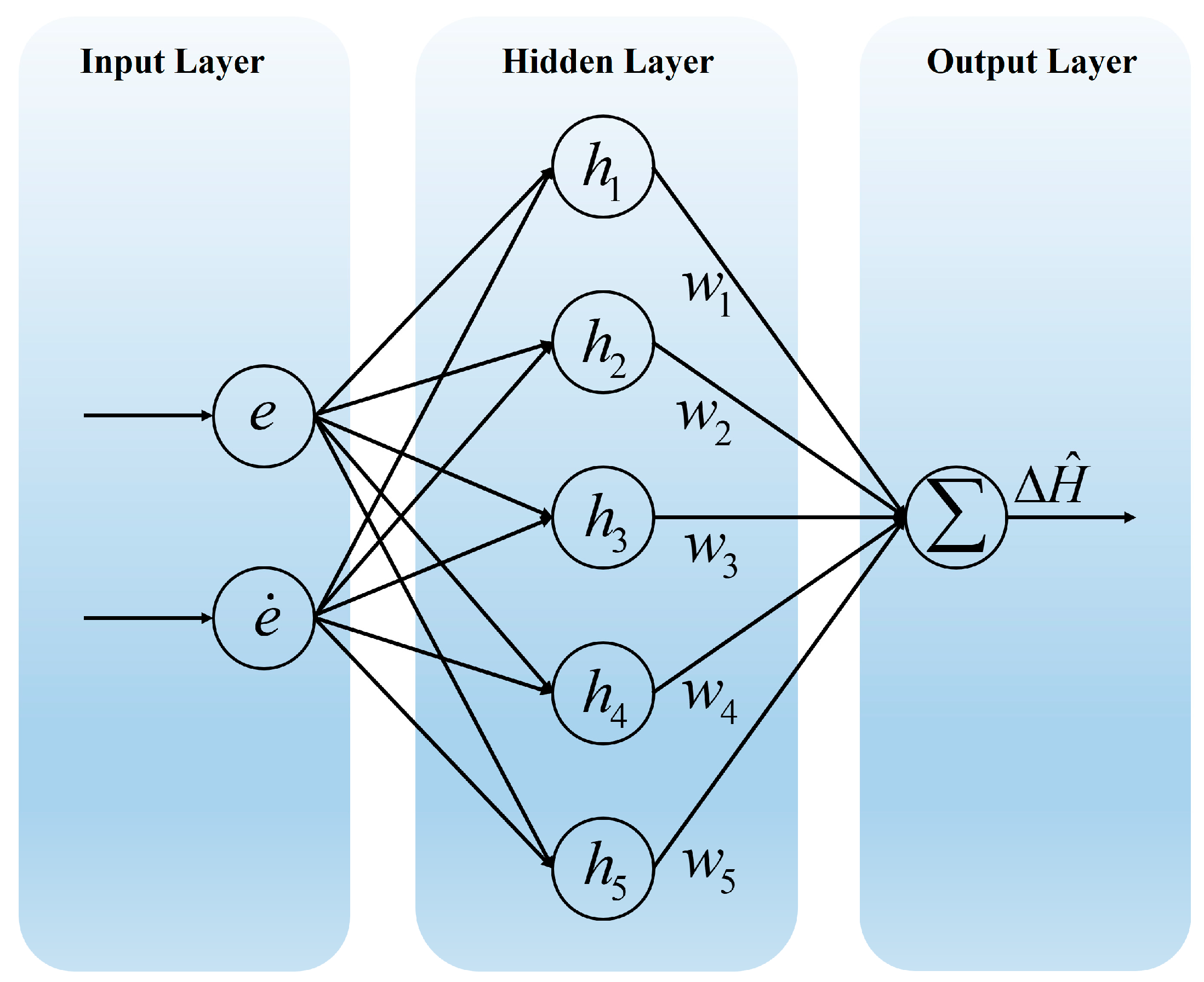
To compensate for the time-delay estimation error, this study used an RBF neural network. It is very difficult to mathematically define time-delay estimation error. However, RBF neural networks are independent of control systems and allow for the estimation of time-delay estimation errors without complex mathematical analysis. In this study, we estimated the time-delay estimation error using the same 2-5-1 network structure as in previous research cases [29,30].
Figure 2 is the network structure used in this study, where e = e z   e ϕ   e θ   e   ψ T , e ˙ = e ˙ z   e ˙ ϕ   e ˙ θ   e ˙   ψ T , h i is the activation function output, and w i is weight value. The activation function was a Gaussian function and was expressed as Equation (11).
h i j = exp ( x i c j 2 / 2 b j 2 )
where x i is a Gaussian function input, c j represents the coordinate value of the center point of the Gaussian function, and b j represents the width of the Gaussian function. The output of this neural network could be expressed as Equation (12).
Δ H ^ = W ^ T H ( E )
where W ^ = [ w 1 w 5 ] is the weight vector, H = [ h 1 h 5 ] T is the activation function output vector, and E is the input vector.
Δ H ¯ = W ¯ T H ( E ) + ε
Equation (13) is the optimal time-delay estimation error: W ¯ is the optimal weight vector and ε is the neural network estimation error. To design the weight update law, we utilized Equation (10) and considered Equation (14), which was an error state space model.
E ˙ i = A E i + B · Δ H ~ i
where A is the desired error dynamics control gain matrix and P is the positive definite constant matrix that satisfied Equation (15).
A T P + P A = Q
Matrix Q is explicitly defined as a positive definite matrix.
W ^ ˙ = γ ( E i T P B H ( E ) σ W ~ )
Equation (16) presents a weight update law formulated on the principles of Lyapunov stability without differentiation of the activation function. In this equation, W ~ = W ^ W ¯ represents the weight error vector and both γ and σ are positive control gains.

3.3. Adaptive Robust Term

Robust terms are used to increase the robustness of control systems using neural networks [29,30,31,32,33,34,35]. A robust term consists of a constant control gain and an error sign function similar to the switching term of sliding mode control. This control technique is effective in improving control performance by compensating for estimation errors in controllers using neural networks. However, it cannot respond to large signal changes and, even if it has reached a steady state, it can affect control performance by generating unnecessary control input. We propose an adaptive robust term that combines a robust term with a filter that can adaptively generate signals and remove unnecessary inputs in the steady state.
To design the adaptive robust term, we redefined the optimal time-delay estimation error as Equation (17).
Δ H ¯ = W ¯ T H ( E ) + ε ¯
ε ¯ denotes the optimal neural network estimation error. The adaptive robust term proposed in this paper compensated for neural network estimation error and increased the robustness of the control system.
s = μ 1 E + μ 2 E ˙
Equation (18) is the error surface for designing the adaptive term; μ is control gain. We approximated the nonlinearity of the neural network estimation error as the product of a nonlinear term and an error surface. Therefore, optimal neural network estimation error could be regarded as ε ¯ = ρ ¯ · s . The adaptive robust term proposed in this paper is Equation (19), which was defined as the approximate neural network estimation error ε ^ .
ε ^ = ρ ^ s
ρ ¯ is an optimal nonlinear term; ρ ^ is an approximated nonlinear term.
ρ ^ ˙ = κ ( E i T P B s β ρ ~ )
where ρ ~ = ρ ^ ρ ¯ and β is positive control gain. Equation (20) is a nonlinear term update law designed based on Lyapunov stability.

3.4. Proposed Controller Design

We designed the controller by integrating the previously proposed I-PID controller, RBF neural network, and adaptive robust term.
u ( t ) u ( t h ) M ¯ X ¨ Linearization   of   the   Plant   + M ¯ X ¨ d + K P e ( t ) + K I e ( τ ) d τ + K D e ˙ ( t ) Desired   error   dynamics + M ¯ · Δ H ^ RBF   neural   network + M ¯ · ε ^ Adaptive   robust   term
Equation (21) is the control input including RBF neural network output and the adaptive robust term. Using Equation (21), we could obtain closed-loop error dynamics such as Equation (22).
E ˙ i = A E i + B N
N = W ~ H E i + ρ ~ s . Next, we considered the Lyapunov function candidate that could represent the control system, such as Equation (23).
V = E i T P E i / 2 + W ~ T W ~ / 2 γ + ρ ~ T ρ ~ / 2 κ
Its time derivative was Equation (24).
V ˙ = E ˙ i T P E i / 2 + E i T P E ˙ / 2 + W ~ T W ^ ˙ / γ + ρ ~ T ρ ^ ˙ / κ = A E i + B N P E i / 2 + E i T P A E i + B N / 2 + W ~ T W ^ ˙ / γ + ρ ~ T ρ ^ ˙ / κ = E i T A T P + P A E i / 2 + E i T P N + W ~ T W ^ ˙ / γ + ρ ~ T ρ ^ ˙ / κ = E i T Q E i / 2 E i T P W ~ T B H E + W ~ T W ^ ˙ / γ E i T P B ρ ~ T s + ρ ~ T ρ ^ ˙ / κ = E i T Q E i / 2 W ~ T ( E i T P B H ( E ) W ^ ˙ / γ ) ρ ~ T ( E i T P B s ρ ^ ˙ / κ )
Using Equations (16) and (17), we could obtain Equation (25), which satisfied the Lyapunov stability condition.
V ˙ = E i T Q E i / 2 σ W ~ T W ~ β ρ ~ T ρ ~ 0
The proposed control method satisfied the Lyapunov stability condition. However, adaptive robust terms can cause unnecessary control input in a steady state. This situation may adversely affect control performance. Therefore, the reverse saturation filter was used in the adaptive robust term to prevent this.
s a t r e v ( u ) = u 0 + u if : if : if : u < N N u N u > N
The reverse saturation filter was defined as Equation (26), and the adaptive robust term operated for errors above the threshold value and removed unnecessary control input for errors below the threshold value. The proposed adaptive robust term applying this filter could be defined as ε ^ s a t r e v ( ε ^ ) .
The optimal weights and optimal nonlinear terms were unknown. Therefore, the weight error and nonlinear term error in the weight update rule and nonlinear term update rule could not be known. For this reason, W ~ = W ^ W ¯ and ρ ~ = ρ ^ ρ ¯ could not be included in the update law. We replaced W ^ and ρ ^ . These values were associated with W ~ and ρ ~ and would not result in large values since they were coupled with the I-PID controller. The modified update law used is shown in Equations (27) and (28).
W ^ ˙ = γ ( E i T P B H ( E ) σ W ^ )
ρ ^ ˙ = κ ( E i T P B s β ρ ^ )
Finally, the proposed control input is shown in Equation (29).
u t = u ( t h ) M ¯ X ¨ Linearization   of   the   Plant   + M ¯ X ¨ d + K P e ( t ) + K I e ( τ ) d τ + K D e ˙ ( t ) Desired   error   dynamics + M ¯ · Δ H ^ RBF   neural   network + M ¯ · ε ^ Adaptive   robust   term   with   filter

3.5. Stability Analysis

This study used a modified neural network update law to generate the proposed control inputs and applied a reverse saturation filter to the adaptive robust term to remove unnecessary control inputs in the steady state. In this chapter, we prove that the proposed controller satisfies stability. The proposed controller was composed of three parts: an I-PID controller, an RBF neural network for compensated time-delay estimation error, and an adaptive robust term for increased robustness of the control system. To remove unnecessary control inputs, we used a reverse saturation filter. For this filter, the presence or absence of an adaptive robust term was determined based on the threshold value. Therefore, the stability proof was divided into two parts: above and below the threshold value.
First, we considered when the system error was larger than the threshold value. To investigate control system stability, this study defined the Lyapunov function candidate as in Equation (30).
V ( t ) = E i T P E i / 2 + W ~ T W ~ / 2 γ + ρ ~ T ρ ~ / 2 κ
The Equation (30) time derivative was Equation (31).
V ˙ ( t ) = E ˙ i T P E i / 2 + E i T P E ˙ / 2 + W ~ T W ^ ˙ / γ + ρ ~ T ρ ^ ˙ / κ
By applying the proposed control input from Equation (29), we derived Equation (32).
V t ˙ = E i T A T P + P A E i / 2 σ W ~ T W ~ + W ~ T W ^ + W ~ T W ¯ / 2 β ρ ~ T ρ ~ + ρ ~ T ρ ^ + ρ ~ T ρ ¯ E i T P A T + A + λ m I λ m I E i / 2 σ W ~ T W ~ W ¯ T W ¯ / 2 β ρ ~ T ρ ~ ρ ¯ T ρ ¯ / 2 = λ m E i T P E i / 2 + E i T P A T + A + λ m I E i / 2 σ W ~ T W ~ W ¯ T W ¯ / 2 β ρ ~ T ρ ~ ρ ¯ T ρ ¯ / 2
If λ m satisfied λ m > 0 , I was a 3 × 3 unit matrix. The control gain was equal to σ λ m / γ and β λ m / κ , and we could obtain Equation (33).
V ˙ ( t ) λ m E i T P E i / 2 + E i T P λ m I E i / 2 σ W ~ T W ~ W ¯ T W ¯ / 2 β ρ ~ T ρ ~ ρ ¯ T ρ ¯ / 2 λ m ( E i T P E i / 2 + W ~ T W ~ / 2 γ + ρ ~ T ρ ~ / κ ) + E i T P λ m I E i / 2 + λ m W ¯ T W ¯ / 2 + λ m ρ ¯ T ρ ¯ / 2 λ m V + Φ
Defining Φ = E i T P λ m I E i / 2 + λ m W ¯ T W ¯ / 2 + λ m ρ ¯ T ρ ¯ / 2 and utilizing Equation (33), we could derive Equation (34).
V ( t ) V t 0 Φ / λ m e λ m ( t N t 0 ) + Φ / λ m
t 0 represents the initial time and t N denotes the time when the system error reaches a threshold value. Through Equations (3)–(34), we could verify that the proposed control system was bounded when it was larger than the threshold value.
Next, we considered when the system error was lower than the threshold value. To verify stability, we considered the Lyapunov function candidate as in Equation (35).
V ( t ) = E i T P E i / 2 + W ~ T W ~ / 2 γ
The Equation (35) time derivative was Equation (36).
V ˙ ( t ) = E ˙ i T P E i / 2 + E i T P E ˙ / 2 + W ~ T W ^ ˙ / γ
Using the proposed control input Equation (29) without the adaptive robust term, we obtained Equation (37).
V t ˙ = E i T A T P + P A E i / 2 σ W ~ T W ~ + W ~ T W ^ + W ~ T W ¯ / 2 + E i T P B ε   E i T P A T + A + λ m I λ m I E i / 2 σ W ~ T W ~ W ¯ T W ¯ / 2 = λ m E i T P E i / 2 + E i T P A T + A + λ m I E i / 2 σ W ~ T W ~ W ¯ T W ¯ / 2
When below the threshold value, it was assumed that ε approximated zero. If λ m satisfied λ m > 0 , I was a 3 × 3 unit matrix. The control gain was equal to σ λ m / γ , and we could obtain Equation (38).
V ˙ ( t ) λ m E i T P E i / 2 + E i T P λ m I E i / 2 σ W ~ T W ~ W ¯ T W ¯ / 2 λ m ( E i T P E i / 2 + W ~ T W ~ / 2 γ ) + E i T P λ m I E i / 2 + λ m W ¯ T W ¯ / 2 λ m V + Φ ˘
Defining Φ ˘ = E i T P λ m I E i / 2 + λ m W ¯ T W ¯ / 2 and utilizing Equation (37), we could derive Equation (39).
V ( t ) V t N Φ ˘ / λ m e λ m ( t t N ) + Φ ˘ / λ m
According to Equation (39), it was bounded even below the threshold value. Using the reverse saturation filter, this system was not smooth and had two bounds. However, as both cases were bounded, the whole control system was confirmed to be asymptotically stable [29,30,40,41,42].

4. Simulation

4.1. Simulation Setup

Computer simulations were performed to verify the performance of the proposed controller. The quadrotor parameters [43] used in the simulation are listed in Table 1.
The control parameters are shown in Table 2, and the sampling time was 0.001 s. All control parameters were determined through iterative simulations. The parameter determination process was a step-by-step tuning process starting from I-PID. The RBF neural network initial weight W = 0.1 ,   0.01 ,   0.1 ,   0.01 ,   0.1 , c = 1 ,   0.5 ,   0 ,   0.5 ,   1 , and b = 15 .
The relationship between the control input and the angular velocity of the rotor was defined as Equation (40).
u z u ϕ u θ u ψ = b b b b l b 0 l b 0 0 l b 0 l b d d d d ω 1 2 ω 2 2 ω 3 2 ω 4 2
where d is the drag factor and Ω ¯ = ω 1 ω 2 + ω 3 ω 4 . The path equation set to follow a continuous helical path in the simulation is given in Equation (41). In this simulation, effects such as disturbances, model uncertainty, and noise were considered lumped disturbances. Therefore, the lumped disturbance used a complex disturbance including disturbance proportional to the velocity term, a sinusoidal signal, and a constant bias, and was defined as Equation (42) and applied to the quadrotor.
x r = 1 e 0.5 t · sin t y r = 1 e 0.5 t · cos t z r = 0.1 t ψ r = 1
D x = k d r a g · x ˙ + 2 sin 1.5 t + 0.8 D y = k d r a g · y ˙ + 4 sin 2 t + 0.7 D z = k d r a g · z ˙ + 3 sin 3 t + 1.5 D ϕ = k d r a g · ϕ ˙ + 3 sin 2 t + 0.9 D θ = k d r a g · θ ˙ + 3 sin 3 t + 0.7 D ψ = k d r a g · ψ ˙ + 3 sin 1.5 t + 0.8
k d r a g was set at 0.9, defining the drag coefficient. The threshold value for input saturation was 10.
Quadrotor systems inherently pose an underactuated problem, which complicates position control using conventional controllers. Typically, quadrotor systems resolve this issue by employing coupling equations that enable movement along the x and y axes through control inputs ϕ d and θ d . There are research examples for this coupling equation [8,9,10,15,16,43]. One method to achieve this is through the relationship with dynamics and another method is to design a controller. This study utilized a coupling equation for ϕ r and θ r , as presented in Equation (43), to avoid additional controller design.
s i n ϕ = x ¨ s i n ψ y ¨ c o s ψ v z , t a n θ = x ¨ c o s ψ + y ¨ s i n ψ z ¨ + g
The quadrotor, θ , and ϕ needed to remain around zero to maintain the quadrotor attitude. Additionally, to track the x and y axes, we utilized the error signal and the coupling equation, such as Equation (44), similar to the existing quadrotor PD control system.
ϕ d = x e s i n ψ y e c o s ψ v e , θ d = x e c o s ψ + y e s i n ψ z e + g
The whole quadrotor control diagram for simulation is shown in Figure 3. The quadrotor dynamics part contains thruster information and input saturation.

4.2. Simulation Results

This chapter presents the simulation results using the parameters and control system covered in Section 4.1 The initial value of the quadrotor was x = 0.3 ,   y = 0.2 ,   z = 0 ,   ϕ = 0.05 ,   θ = 0.035 ,   ψ = 0 .
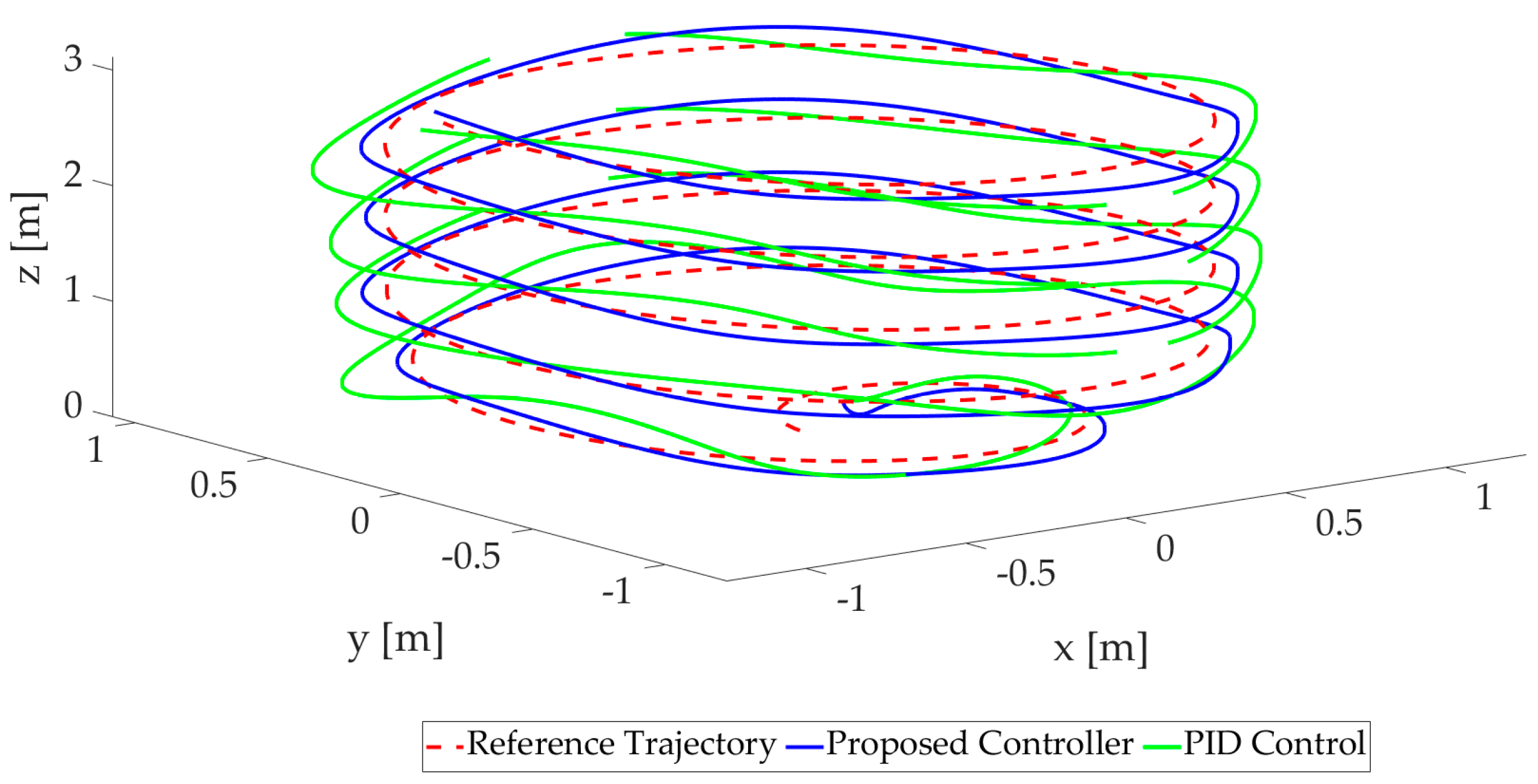
Figure 4 illustrates the tracking performance of both the proposed controller and the PID control when following the reference trajectory. As indicated by the results, both controllers were capable of maintaining effective tracking performance, even in environments with disturbances. These outcomes confirm that both the traditional PID control system and the coupling equations used effectively managed the control tasks. However, the PID control was slightly wider in the x and y axes in the reference trajectory than the proposed controller. This means that the proposed controller showed better tracking performance compared to the PID control. Therefore, the next section discusses the position and posture tracking performance of the proposed controller and PID control.

4.2.1. Position Control Simulation Results

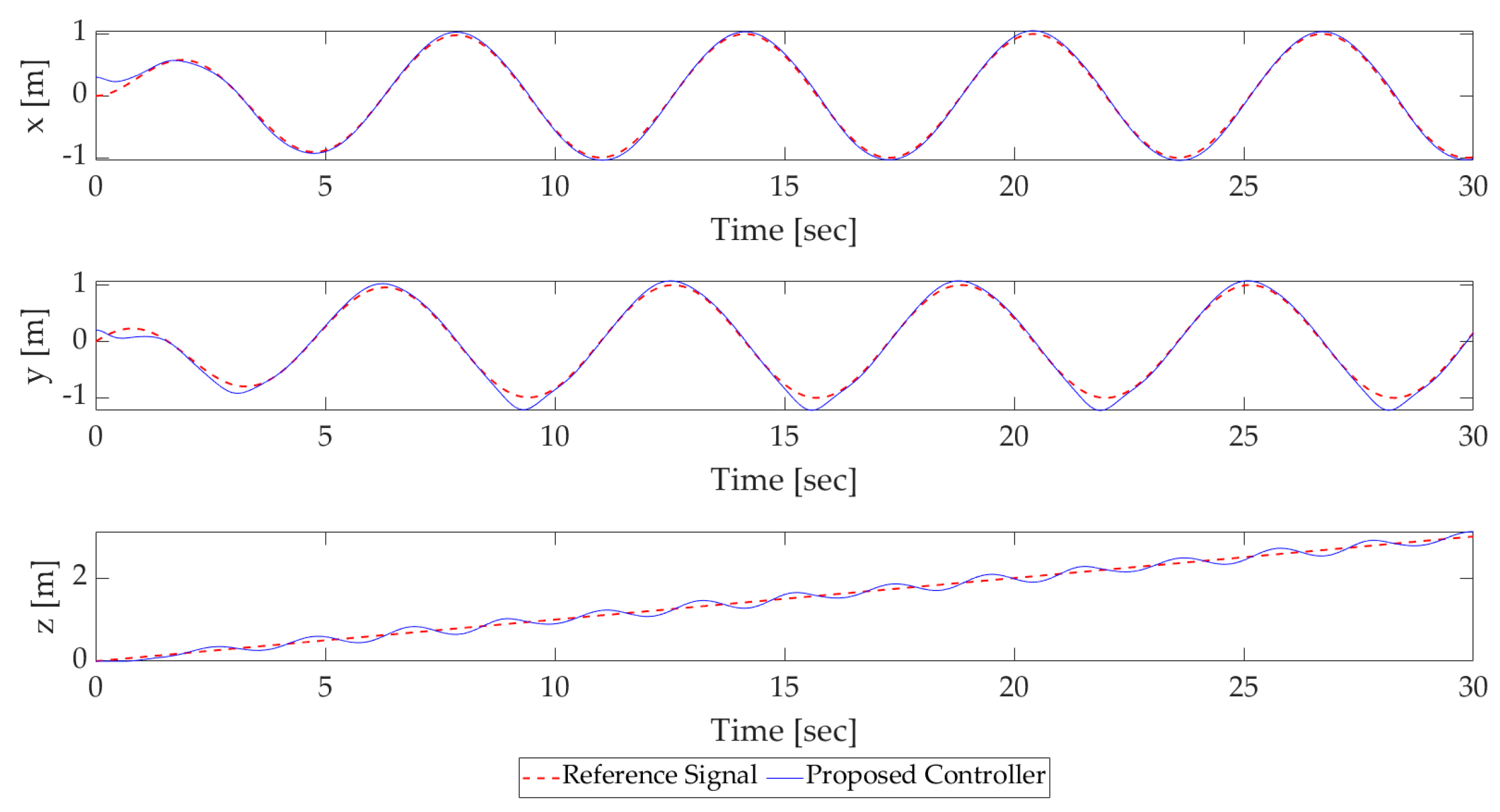
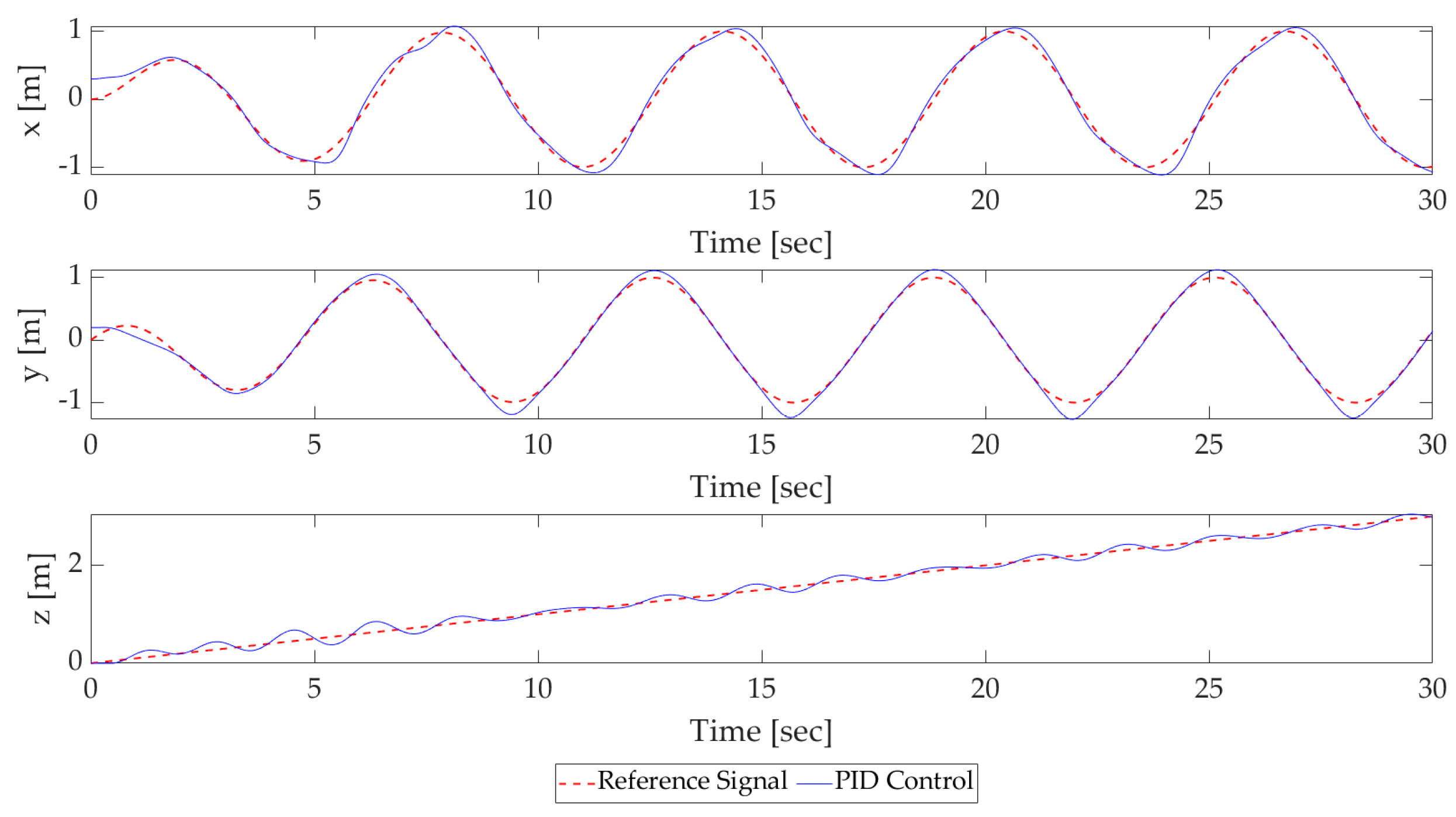
This chapter presents the position control simulation results using the proposed controller. Figure 5 illustrates the position tracking performance of the proposed controller, while Figure 6 displays the performance of the PID control. The results depicted in Figure 5 and Figure 6 demonstrate good tracking performance across all three axes. First, we see that the tracking performance for the X-axis of the proposed controller converged to the reference trajectory at 1.145 s. The maximum error that occurred was 0.05, which shows that the error was well suppressed. On the other hand, with the PID control, the X-axis converged to the reference trajectory at 1.532 s. The maximum error that occurred was 0.125. Next, the Y-axis tracking performance of the proposed controller showed that it converged to the reference trajectory in 1.449 s. The maximum error was 0.221, which was larger than for the X-axis error but smaller overall, showing satisfactory performance. The performance of the PID control was also satisfactory, converging to the reference trajectory in 1.844 s. The maximum error that occurred was 0.236. Z-axis tracking performance was different from the x-axis and y-axis. Based on the maximum error amplitude occurring below 0.2, the tracking performance of the proposed controller was found to reach near the reference trajectory in 1.5 s. The error was 0.117, and it can be seen that it operated around the reference trajectory. PID control also operated based on the reference trajectory and converged in 6.316 s, with an error of 0.161. A detailed comparison can be seen in the error comparison in Figure 7. As can be seen from the position control results, the x-axis tracking performance was noticeably improved, and the impact on the y and z axes was slightly improved, showing that all three axes could be improved.

4.2.2. Attitude Control Simulation Results

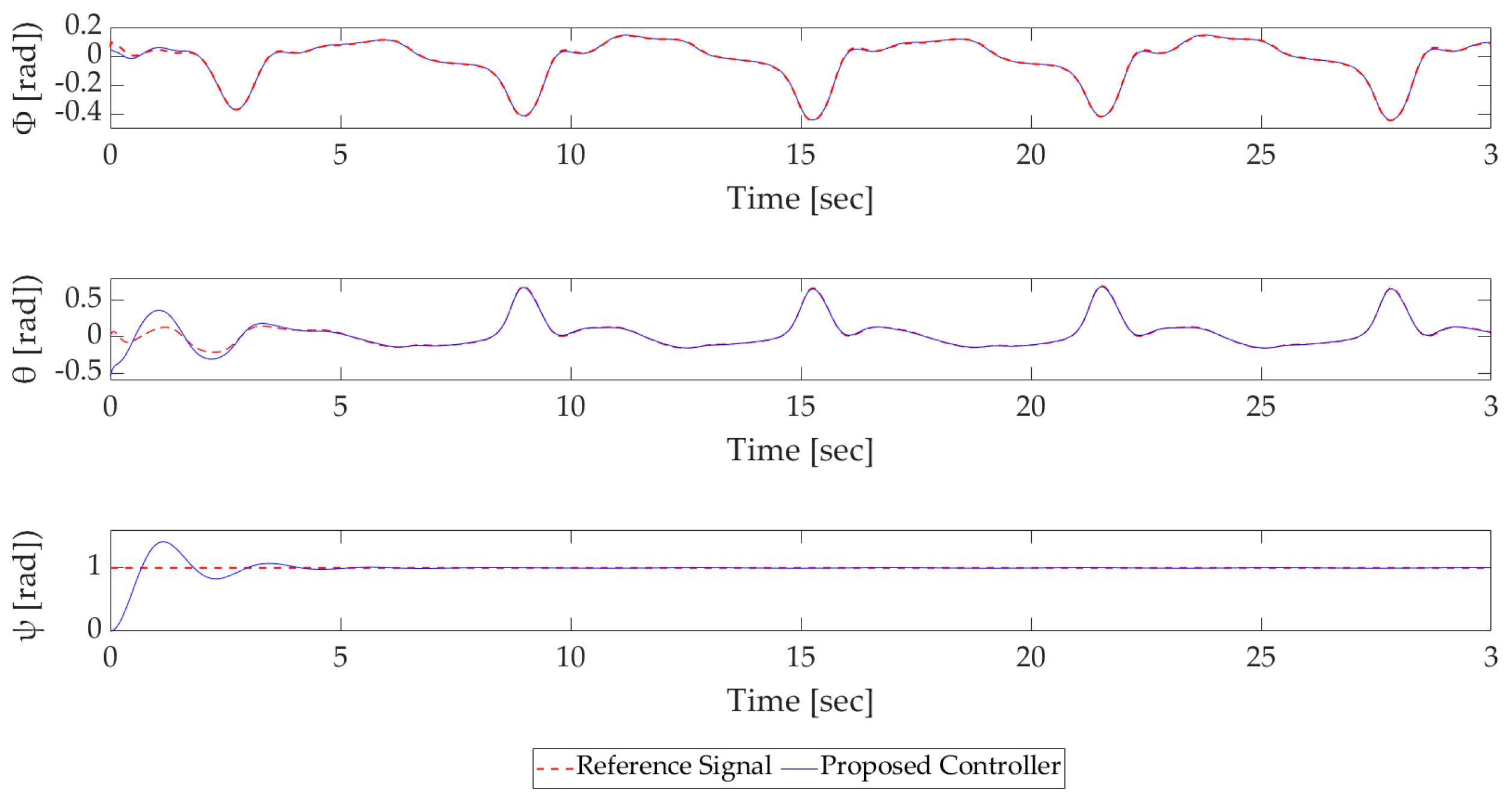
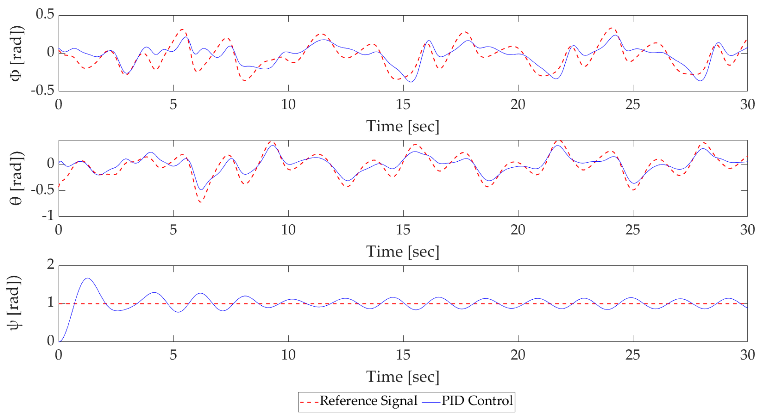
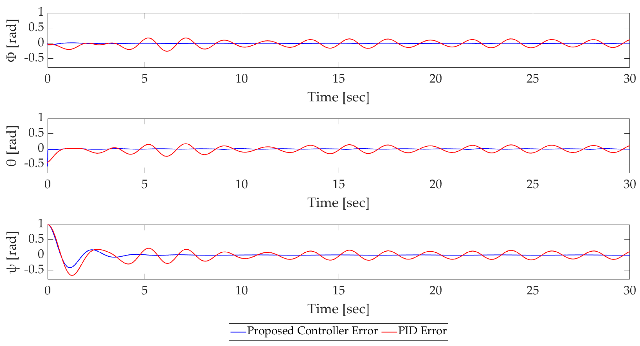
This chapter presents the attitude control simulation results for both the proposed controller and the traditional PID control. The reference signal ϕ d ,   θ d was generated by the position PD controller. Consequently, the expression of the reference signal varied based on the tracking performance of each controller. Figure 8 and Figure 9 illustrate the attitude tracking performance of the proposed controller and the PID control, respectively, while Figure 10 compares the attitude error performance between the two controllers. At ϕ , the proposed controller began to converge in 1.9 s and showed excellent tracking performance, with a maximum error of 0.008. On the other hand, although the PID control could respond to changes in signals, it did not have excellent tracking performance. The maximum error was 0.173. At θ , it converged from about 2.6 s. The maximum error occurred at 0.25. After 2.6 s, the tracking performance error rapidly decreased and converged. In the case of the PID control, the convergence speed was 2 s faster than that of the proposed controller. However, compared to the proposed controller, the tracking performance was insufficient, and a large error occurred during operation, with a maximum error of 0.142.
ψ exhibited similar behavior characteristics to a second-order system. The maximum %overshoot was 39% and converged to a steady state around 2.7 s. After convergence, it had high tracking performance. For the PID control, the maximum %overshoot was 66% and ranged between 0.088 and 0.117 from around 8.5 s.
Figure 11 shows the control input comparison results when the proposed controller and the quadrotor system using PID control tracked the reference trajectory. The control input aspect was similar for both controllers. In particular, as shown in U θ , the proposed controller could generate large inputs at the beginning of an operation that required a lot of tracking performance or when control inputs were required. Additionally, when entering a steady state, it could be confirmed that phenomena such as chattering caused by unnecessary control input did not occur due to the reverse saturation filter.
Consequently, the proposed control system enabled the design of a control system based on a model-free technique similar to the conventional PID control, and it was confirmed that it could enhance tracking performance.

5. Conclusions

In this paper, an I-PID controller was utilized that was similar to the PID controller widely used in previous quadrotor systems and showed high robustness. To enhance the robustness of the control system, the time-delay estimation error was compensated for with an RBF neural network. To address the shortcomings of neural network systems and construct a more robust controller, this paper proposed an adaptive robust term. This additional control input included an adaptative term to respond to large signal changes. It was combined with a reverse saturation filter to remove unnecessary control input in a steady state. The adaptive law of the proposed controller was designed based on Lyapunov stability to satisfy stability. The stability of the entire control system was proven by examining the boundary based on the reverse saturation filter section.
To verify the control system, simulations were performed on a quadrotor navigating a spiral path, subjected to 6-axis lumped disturbances. A conventional PID controller, commonly employed in quadrotor systems, served as the baseline for comparison. The simulation results demonstrated that the overall tracking performance of the proposed controller was superior to that of the PID control. With the proposed controller, convergence was achieved within 3 s across all six axes, with the error being reduced to as low as 0.23. Consequently, the controller introduced in this paper could be configured similarly to the conventional PID controller, yet it exhibited satisfactory performance.
In the future, we plan to make a quadrotor system to experimentally verify the controller and then conduct tracking experiments using a GPS (Global Positioning System) and hovering performance tests in situations where disturbances exist.

Author Contributions

S.-J.K. contributed to the conception of the study, designed the control system, performed the experiment, performed the data analyses, and wrote the manuscript; J.-H.S. contributed to the conception of the study, helped to write the manuscript, helped perform the analysis, and participated in constructive discussions corresponding the manuscript. All authors have read and agreed to the published version of the manuscript.

Funding

This work was supported by the Ministry of Trade, Industry & Energy (MOTIE, Korea) under the Industrial Technology Innovation Program, grant no. 20026194, “Development of Human-Life Detection and Fire-Suppression Solutions based on Quadruped Robots for Firefighting and Demonstration of Firefighting Robots and Sensors”.

Institutional Review Board Statement

Not applicable.

Informed Consent Statement

Not applicable.

Data Availability Statement

The original contributions presented in the study are included in the article, further inquiries can be directed to the corresponding author.

Conflicts of Interest

The authors declare no conflicts of interest.

References

  1. Petrlík, M.; Báča, T.; Heřt, D.; Vrba, M.; Krajník, T.; Saska, M. A Robust UAV System for Operations in a Constrained Environment. IEEE Robot. Autom. Lett. 2020, 5, 2169–2176. [Google Scholar] [CrossRef]
  2. Huang, Y.; Meng, Z. Bearing-based distributed formation control of multiple vertical take-off and landing UAVs. IEEE Trans. Control Netw. 2021, 8, 1281–1292. [Google Scholar] [CrossRef]
  3. Hu, J.; Zhang, H.; Song, L.; Schober, R.; Poor, H.V. Cooperative Internet of UAVs: Distributed trajectory design by multi-agent deep reinforcement learning. IEEE Trans. Commun. 2020, 68, 6807–6821. [Google Scholar] [CrossRef]
  4. Xu, L.; Qin, K.; Tang, F.; Shi, M.; Lin, B. UDE-Based Dynamic Surface Control for Quadrotor Drone Attitude Tracking under Non-Ideal Actuators. Drones 2023, 7, 305. [Google Scholar] [CrossRef]
  5. He, Z.; Hu, J.; Wang, Y.; Cong, J.; Bian, Y.; Han, L. Attitude-Tracking Control for Over-Actuated Tailless UAVs at Cruise Using Adaptive Dynamic Programming. Drones 2023, 7, 294. [Google Scholar] [CrossRef]
  6. Shen, Z.; Tsuchiya, T. Singular Zone in Quadrotor Yaw–Position Feedback Linearization. Drones 2022, 6, 84. [Google Scholar] [CrossRef]
  7. Yogi, S.C.; Tripathi, V.K.; Behera, L. Adaptive Integral Sliding Mode Control Using Fully Connected Recurrent Neural Network for Position and Attitude Control of Quadrotor. IEEE Trans. Netw. Learn. Syst. 2021, 32, 5595–5609. [Google Scholar] [CrossRef]
  8. Hu, M.; Ahn, H.; You, K. Finite-Time Rapid Global Sliding-Mode Control for Quadrotor Trajectory Tracking. IEEE Access 2023, 11, 22364–22375. [Google Scholar] [CrossRef]
  9. Sun, J.; Wang, Y.; Yu, Y.; Sun, C. Nonlinear Robust Compensation Method for Trajectory Tracking Control of Quadrotors. IEEE Access 2019, 7, 26766–26776. [Google Scholar] [CrossRef]
  10. Ullah, S.; Mehmood, A.; Khan, Q.; Rehman, S.; Iqbal, J. Robust Integral Sliding Mode Control Design for Stability Enhancement of Under-actuated Quadrotor. Int. J. Control Autom. Syst. 2020, 18, 1671–1678. [Google Scholar] [CrossRef]
  11. Yu, G.; Reis, J.; Silvestre, C. Quad Neural Network Adaptive Control: Design and Experimental Validation. IEEE Robot. Autom. Lett. 2023, 8, 2574–2581. [Google Scholar] [CrossRef]
  12. Ouyang, Y.; Xue, L.; Dong, L.; Sun, C. Neural Network-Based Finite-Time Distributed Formation-Containment Control of Two Layer Quadrotor UAVs. IEEE Trans. Syst. Man Cybern. Syst. 2022, 52, 4836–4848. [Google Scholar] [CrossRef]
  13. Liu, H.; Xi, J.; Zhong, Y. Robust Attitude Stabilization for Nonlinear Quadrotor Systems with Uncertainties and Delay. IEEE Trans. Ind. Electron. 2017, 64, 5585–5595. [Google Scholar] [CrossRef]
  14. Tayebi, A.; McGilvray, S. Attitude stabilization of a VTOL quadrotor aircraft. IEEE Trans. Control Syst. Technol. 2006, 14, 562–571. [Google Scholar] [CrossRef]
  15. Alexis, K.; Nikolakopoulos, G.; Tzes, A. Switching model predictive attitude control for a quadrotor helicopter subject to atmosphere disturbance. Control Eng. Pract. 2011, 10, 1195–1207. [Google Scholar] [CrossRef]
  16. Li, J.; Zhang, G.; Zhang, X.; Zhang, W. Integrating Dynamic Event-Triggered and Sensor-Tolerant Control: Application to USV-UAVs Cooperative Formation System for Maritime Parallel Search. IEEE Trans. Intell. Transp. Syst. 2023, 1–13. [Google Scholar] [CrossRef]
  17. Li, J.; Zhang, G.; Zhang, W.; Shan, Q.; Zhang, W. Cooperative Path Following Control of USV-UAVs Considering Low Design Complexity and Command Transmission Requirements. IEEE Trans. Intell. Transp. Syst. 2023, 9, 715–724. [Google Scholar] [CrossRef]
  18. Fliess, M.; Join, C. Intelligent PID controller. In Proceedings of the 2008 16th Mediterranean Conference on Control and Automation, Ajaccio, France, 25–27 June 2008; pp. 326–331. [Google Scholar]
  19. Wang, J.; Mounier, H.; Cela, A.; Niculescu, S. Event-driven intelligent PID controllers with applications to motion control. In Proceedings of the 18th IFAC World Congress, Milan, Italy, 28 August–2 September 2011; pp. 10080–10085. [Google Scholar]
  20. Choe, Y. Optimal Tuning Strategy for 2-Degree-of-Freedom I-PID Controllers. Trans. Korean Inst. Electr. Eng. 2018, 67, 1202–1209. [Google Scholar]
  21. Jung, S. A Neural Network Technique of Compensating for an Inertia Model Error in a Time-delayed Controller for Robot Manipulators. Int. J. Control Autom. Syst. 2020, 18, 1863–1871. [Google Scholar] [CrossRef]
  22. Han, S.; Tian, Y.; Christov, N.; Wang, H. Time-delay estimation based computed torque control with robust adaptive RBF neural network compensator for a rehabilitation exoskeleton. ISA Trans. 2020, 97, 171–181. [Google Scholar] [CrossRef]
  23. Slama, S.; Errachdi, A.; Benrejeb, M. Neural adaptive PID and neural indirect adaptive control switch controller for nonlinear MIMO systems. Math. Probl. Eng. 2019, 2019, 7340392. [Google Scholar] [CrossRef]
  24. Ge, S.; Wang, C. Direct adaptive NN control of a class of nonlinear systems. IEEE Trans. Neural Netw. 2002, 15, 214–221. [Google Scholar] [CrossRef] [PubMed]
  25. Ong, Q.; Yin, L. Robust adaptive fault accommodation for a robot system using a radial basis function neural network. Int. J. Syst. Sci. 2010, 32, 195–204. [Google Scholar]
  26. Liu, J. Intelligent Control Design and MATLAB Simulation; Springer: Berlin/Heidelberg, Germany, 2018; pp. 113–233. [Google Scholar]
  27. Seghouane, A.; Shokouhi, N. Adaptive Learning for Robust Radial Basis Function Networks. IEEE Trans. Cybern. 2021, 51, 2847–2856. [Google Scholar] [CrossRef] [PubMed]
  28. Liu, J. Radial Basis Function (RBF) Neural Network Control for Mechanical Systems: Design, Analysis and Matlab Simulation; Springer: Berlin/Heidelberg, Germany, 2018; pp. 1–280. [Google Scholar]
  29. Kim, S.; Jin, M.; Suh, J. A Study on the Design of Error-Based Adaptive Robust RBF Neural Network Back-Stepping Controller for 2-DOF Snake Robot’s Head. IEEE Access 2023, 11, 23146–23156. [Google Scholar] [CrossRef]
  30. Kim, S.; Suh, J. Adaptive Robust RBF-NN Nonsingular Terminal Sliding Mode Control Scheme for Application to Snake Robot’s Head for Image Stabilization. Appl. Sci. 2023, 13, 4899. [Google Scholar] [CrossRef]
  31. Wan, M.; Chen, M.; Lungu, M. Integral Backstepping Sliding Mode Control for Unmanned Autonomous Helicopters Based on Neural Networks. Drones 2023, 7, 154. [Google Scholar] [CrossRef]
  32. Cao, X.; Shi, P.; Li, Z.; Liu, M. Neural-network-based adaptive backstepping control with application to spacecraft attitude regulation. IEEE Trans. Neural Netw. Learn. Syst. 2018, 29, 4303–4313. [Google Scholar] [CrossRef] [PubMed]
  33. Zhang, Y.; Peng, P.; Jiang, Z. Stable neural controller design for unknown nonlinear systems using backstepping. IEEE Trans. Neural Netw. 2000, 11, 1347–1360. [Google Scholar]
  34. Wang, W.; Kuo, M.; Lee, T.; Hong, C.; Leu, Y. RBF neural network adaptive backstepping controllers for MIMO nonaffine nonlinear systems. In Proceedings of the 2009 IEEE International Conference on Systems, Man and Cybernetics, San Antonio, TX, USA, 11–14 October 2009; pp. 4946–4951. [Google Scholar]
  35. Zhu, J.; Cao, Z.; Zhang, T.; Yang, Y.; Yi, Y. Sufficient Condition for the Existence of the Compact Set in the RBF Neural Network Control. IEEE Trans. Neural Netw. Learn. Syst. 2018, 29, 3277–3282. [Google Scholar] [CrossRef]
  36. Bouadi, H.; Mora-Camino, F. Modeling and adaptive flight control for quadrotor trajectory tracking. J. Aircr. 2017, 55, 1–16. [Google Scholar] [CrossRef]
  37. Aboudonia, A.; El-Badawy, A.; Rashad, R. Disturbance observer-based feedback linearization control of an unmanned quadrotor helicopter. Proc. Inst. Mech. Eng. Part J. Syst. Control Eng. 2016, 230, 877–891. [Google Scholar] [CrossRef]
  38. Bouadi, H.; Bouchoucha, M.; Tadjine, M. Sliding Mode Control based on Backstepping Approach for an UAV Type-Quadrotor. Int. J. Mech. Mechatron. Eng. 2007, 1, 39–44. [Google Scholar]
  39. Jung, S. An Impedance Force Control Approach to a Quad-Rotor System Based on an Acceleration-Based Disturbance Observer. J. Intell. Robot. Syst. 2014, 73, 175–185. [Google Scholar] [CrossRef]
  40. Fang, Y.; Fei, J.; Ma, K. Model reference adaptive sliding mode control using RBF neural network for active power filter. Electr. Power Energy Syst. 2015, 73, 249–258. [Google Scholar] [CrossRef]
  41. Liu, Q.; Li, D.; Ouyang, Z.; Tee, K.; Ge, S. Adaptive bias RBF neural network control for a robotic manipulator. Neurocomputing 2021, 447, 213–223. [Google Scholar] [CrossRef]
  42. Wang, L.; Chai, T.; Zhai, L. Neural-Network-Based Terminal Sliding-Mode Control of Robotic Manipulators Including Actuator Dynamics. IEEE Trans. Ind. Electron. 2009, 56, 3296–3304. [Google Scholar] [CrossRef]
  43. Hwang, N.; Kim, B. Active Fault Tolerant Control of Quadrotor Based on Multiple Sliding Surface Control Method. J. KIECS 2022, 17, 59–70. [Google Scholar]
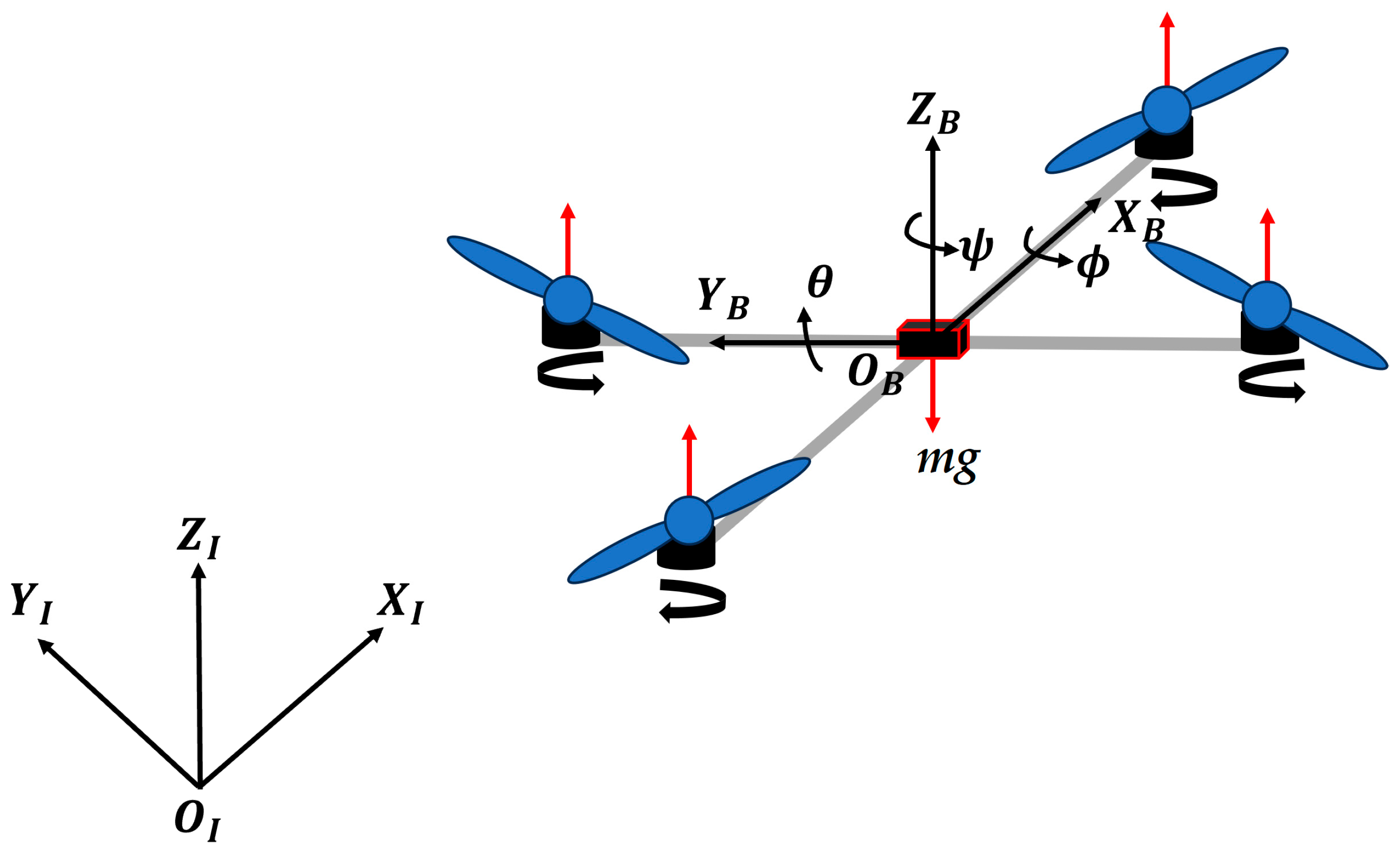
Figure 1. Coordinate system of quadrotor.
Drones 08 00179 g001
Figure 2. RBF neural network structure.
Drones 08 00179 g002
Figure 3. Quadrotor control system structure.
Drones 08 00179 g003
Figure 4. Comparison of 3D trajectory tracking performance using the proposed controller and PID control.
Drones 08 00179 g004
Figure 5. Position tracking performance of the proposed controller.
Drones 08 00179 g005
Figure 6. Position tracking performance of the PID control.
Drones 08 00179 g006
Figure 7. Comparison of the position error performance of the proposed controller and PID control.
Drones 08 00179 g007
Figure 8. Attitude tracking performance of the proposed controller.
Drones 08 00179 g008
Figure 9. Attitude tracking performance of the PID controller.
Drones 08 00179 g009
Figure 10. Comparison of the attitude error performance of the proposed controller and PID control.
Drones 08 00179 g010
Figure 11. Comparison of the control input using the proposed controller and PID control.
Drones 08 00179 g011
Table 1. The quadrotor parameters.
ParameterDescriptionValue
m Mass of quadrotor0.5 k g
I x Moment of inertia about X B 0.0023 k g · m 2
I y Moment of inertia about Y B 0.0023 k g · m 2
I z Moment of inertia about Z B 0.0051 k g · m 2
l Distance between center of the quadrotor and the propeller0.17 m
b Thrust factor0.00018 N · m 2
J r Total moment of inertia of motor0.000065 k g · m 2
gAcceleration of gravity9.81 m / s 2
Table 2. The proposed controller parameters.
ParameterValue
k P 8
k I 0.002
k D 1.6
M ¯ 0.02
P 28.5 0.5 0.5 28.5
γ 0.7
σ 0.2
μ 1 0.5
μ 2 0.2
κ 0.01
β 0.001
N0.1
Disclaimer/Publisher’s Note: The statements, opinions and data contained in all publications are solely those of the individual author(s) and contributor(s) and not of MDPI and/or the editor(s). MDPI and/or the editor(s) disclaim responsibility for any injury to people or property resulting from any ideas, methods, instructions or products referred to in the content.