Manipulating Camera Gimbal Positioning by Deep Deterministic Policy Gradient Reinforcement Learning for Drone Object Detection

Abstract

The object recognition technology of unmanned aerial vehicles (UAVs) equipped with “You Only Look Once” (YOLO) has been validated in actual flights. However, here, the challenge lies in efficiently utilizing camera gimbal control technology to swiftly capture images of YOLO-identified target objects in aerial search missions. Enhancing the UAV’s energy efficiency and search effectiveness is imperative. This study aims to establish a simulation environment by employing the Unity simulation software for target tracking by controlling the gimbal. This approach involves the development of deep deterministic policy-gradient (DDPG) reinforcement-learning techniques to train the gimbal in executing effective tracking actions. The outcomes of the simulations indicate that when actions are appropriately rewarded or penalized in the form of scores, the reward value can be consistently converged within the range of 19–35. This convergence implies that a successful strategy leads to consistently high rewards. Consequently, a refined set of training procedures is devised, enabling the gimbal to accurately track the target. Moreover, this strategy minimizes unnecessary tracking actions, thus enhancing tracking efficiency. Numerous benefits arise from training in a simulated environment. For instance, the training in this simulated environment is facilitated through a dataset composed of actual flight photographs. Furthermore, offline operations can be conducted at any given time without any constraint of time and space. Thus, this approach effectively enables the training and enhancement of the gimbal’s action strategies. The findings of this study demonstrate that a coherent set of action strategies can be proficiently cultivated by employing DDPG reinforcement learning. Furthermore, these strategies empower the UAV’s gimbal to rapidly and precisely track designated targets. Therefore, this approach provides both convenience and opportunities to gather more flight-scenario training data in the future. This gathering of data will lead to immediate training opportunities and help improve the system’s energy consumption.

1. Introduction

During the early stages of the development of artificial intelligence, its progress was limited by computer processing speeds and hardware capabilities. Consequently, it did not gain widespread attention or find extensive applications. However, as computer software and hardware improved and people’s theoretical understanding of artificial intelligence evolved, research and discussions on machine learning were reignited, leading to remarkable breakthroughs. One noteworthy accomplishment is the AlphaGo project initiated by Google DeepMind in 2014. Through continuous refinement and experimentation, AlphaGo triumphed over the world champion, Go, in 2016. This achievement rekindled the interest of numerous scholars and underscored the potency of artificial intelligence and reinforcement-learning methodologies.

For advancing reinforcement-learning algorithms, Volodymyr Mnih et al. [1] introduced the Deep Q Network (DQN) in 2013. DQN melds deep neural networks with Q-learning, constituting a pivotal reinforcement-learning algorithm. The core of this method is the use of a deep neural network referred to as the Q network, which approximates the action-value function, also known as the Q-function. This portrays the anticipated cumulative reward associated with executing a particular action in a given state. In 2014, David Silver et al. [2] proposed a deterministic policy gradient (DPG), which defines policy as a mapping from state to action and achieves optimal policy acquisition by maximizing the projected return. After 2013, DeepMind continued to improve DQN. In 2015, they introduced the Nature version of DQN, published in Nature [3], and proposed three variants: Double DQN, Prioritized Replay, and Dueling Network. In 2016, Mnih et al. introduced the Asynchronous Advantage Actor-Critic (A3C) approach [4], which employs multiple independently operating agents that simultaneously engage with the environment, facilitating parameter updates. This innovative technique enhances both training efficiency and overall performance. In 2017, Bellemare, Dabney, and Munos [5] established the Distributional DQN strategy. Contrary to estimating averages, this technique learns the distribution of discounted returns, thereby offering a unique perspective. That same year, Fortunato et al. [6] presented the Noisy DQN concept. This approach involves incorporating random network layers to facilitate exploration in the learning process. In 2018, DeepMind introduced Rainbow DQN [7], a profound advancement in deep reinforcement learning. Rainbow DQN integrates six considerable enhancements into the DQN framework, namely (1) Double Q-Learning, (2) Prioritized Replay, (3) Dueling Networks, (4) Multistep Learning, (5) Distributional Reinforcement Learning (DRL), and (6) Noisy Nets. Within the Arcade Learning Environment, which is a testing and comparison platform for reinforcement-learning (RL) algorithms, DeepMind employed 57 Atari 2600 games to evaluate Rainbow DQN, the original DQN, and six enhanced DQN agents. Notably, the results outperformed other methods in terms of both data efficiency and outcomes. The effectiveness of combining diverse algorithm strengths has been underscored by these endeavors. This study adopts the deep deterministic policy gradient (DDPG) algorithm, a fusion of DPG and DQN. This combination harnesses the benefits of both techniques, rendering it well-suited for addressing motion challenges in continuous space.

As reinforcement-learning technology experiences breakthroughs, its applications span an extensive array of fields, including control applications. Fernandez-Gauna et al. [8] exemplified this by applying reinforcement learning to enhance the feedback controller for a lead ball-screw feed drive. Their research effectively demonstrated the methodology’s efficacy using two value-iteration methods and three different policy-iteration methods and compared it with the benchmark double-loop proportional-integrated-derivative controllers. In this study, controller parameters were optimized through algorithmic exploration and learning. This iterative process leads to system refinement, improving performance indicators such as positioning accuracy and responsiveness. Huang et al. [9] introduced a novel approach that leverages the reinforcement learning of the DQN algorithm’s reward accumulation and time-difference learning characteristics. After these aspects are iteratively valued to drive optimal decisions, a deep prediction mode is created to estimate the deviation of the XXY platform’s movement and assist in issuing compensation command predictions for error trends. This technique not only offers a fresh shift compensation method but also extends to controller parameter modulation applications. Currently, recent studies are paving RL’s way into the realm of robot control [10,11]. Eric J. Tzeng et al. [12] employed DQN to solve the inverse kinematics conditional-design challenge. Through reinforcement learning, they guided a single-legged machine model to move its endpoint to a target point in a simulation environment while automatically managing intermediate positioning differences. This showcases the model’s capacity to adapt its movements under diverse postures and environmental conditions, effectively achieving accurate target point movement. As for the ground autonomous vehicle, self-driving car system applications using DQN were studied in [13,14]. Yu-Chen Lin et al. [15] introduced a reinforcement learning-driven anti-progressive control approach to enhance the design of full-vehicle active suspension systems, aimed at improving both ride comfort and stability. They also employed the DDPG reinforcement learning scheme for controlling the policy. This replaced the need to calculate the virtual control force using the conventional anti-asymptotic method. This substitution not only simplifies the complexity associated with analytically computing the derivative of the virtual control signal but also upholds system robustness in the face of unexpected disturbances arising from road irregularities. DDQN and RL were used for the control of unmanned aerial vehicles in [16,17]. Hyunsoo Lee et al. [18] used Unity to create a simulation environment for UAVs engaged in targeted attacks. They harnessed the DDPG algorithm, tailored it for continuous spaces, and attained successful task completion through dedicated experiments. Recent studies have fused mobile vehicles with imaging and “You Only Look Once” (YOLO) technology [19,20], engaging in reinforcement learning for target search and tracking.

To emulate more realistic real-world scenarios, in this paper, we integrate UAVs and YOLO technology [21] to capture flight images and observe gimbal movement during actual flights. Additionally, they utilized the Unity ML-Agents open-source plugin within the versatile two-dimensional (2D)/three-dimensional (3D) game engine from Unity Technologies to construct a training environment for simulating the gimbal’s visual input (State). By positioning as the central element within this environment, the agent executes actions and garners rewards (positive or negative). Hence, this endeavor determines optimal actions yielding maximum rewards through ongoing interactions. Finally, this approach establishes a set of action strategies enabling effective gimbal control for target tracking.

The remainder of this paper is organized as follows: Section 2 describes the fundamental principles of reinforcement-learning theory and outlines the techniques and architecture principles of DDPG. Section 3 presents the experimental method. Section 4 presents the experimental results. Finally, Section 5 concludes this paper.

2. Theoretical Discussion

2.1. Reinforcement Learning

RL constitutes a significant branch of machine learning. It is unlike “supervised learning”, which relies on predefined labels for training and is distinct from “unsupervised learning”, which extracts patterns, structure, and associations from unlabeled data. RL focuses on discovering patterns, structures, and associations through interactions within a dynamic environment. It is a goal-oriented learning approach that involves an agent interacting with its environment to learn. For example, while training a pet to perform a handshake, when the pet successfully responds to the handshake command, it receives a positive reward. Conversely, if it fails to execute the command, no reward is granted. Over time, the pet learns that actions aligned with commands yield rewards, leading to gradual behavioral adjustments upon command.

Reinforcement learning consists of these key elements: agent, environment, action, state, reward, and policy. Each function is described as follows.

Agent:

The central learner in reinforcement learning is responsible for engaging with the environment by executing actions and receiving rewards.

Environment:

The external setting is where the agent operates and interacts during the learning process. This could be a real-world scenario or a simulated environment.

Action:

These are the actions to be executed by the agent within the environment. The agent selects actions based on its current state to interact with the environment.

State:

This represents the agent’s condition at a specific point in the environment and reflects the outcome of the agent’s actions and interactions with the environment.

Reward:

The feedback received by the agent following its actions in the current state. Rewards can be positive rewards or negative penalties.

Policy:

The strategy or set of rules that guides the agent’s actions in different environmental states. It is a method of achieving goals by formulating action strategies based on interactions involving the environment, state, and action.

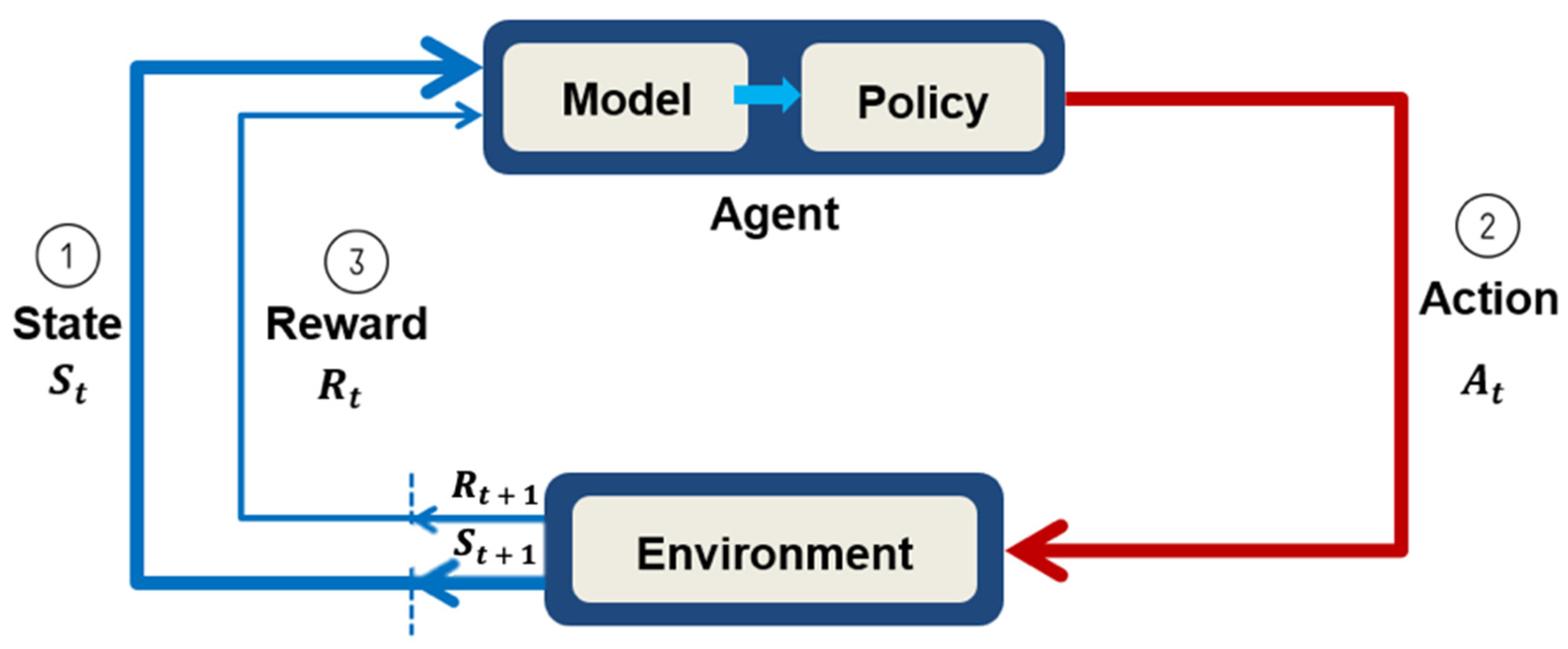
The basic architecture of reinforcement learning is shown in Figure 1. To start, the agent will observe the state of $t$ in the environment at a certain time point ($S_t$) and then choose the corresponding action according to the current state ($a_t$), and the environment will be updated to the next state ($s_{t+1}$). While updating the state, the agent will also receive a reward ($R_{t+1}$), and the agent will evaluate the strategy based on the reward and constantly adjust its strategy to maximize the long-term reward, which is the optimal strategy.

2.2. Markov Decision Process

The Markov decision process model is shown in Figure 2. It is composed of the following five elements:

$S$ is the state set; $P$ is the transition probability of the state; $R$ is the reward function; γ is the discount factor; and $A$ is the action set. Therefore, the state transition function, $P$, used to describe the state transition probability at a certain time point, $\mathrm{t}$, when a specific action is taken can be expressed as Formula (1). $R$ is the reward function, which is used to describe how much reward will be obtained after taking an action and changing the state at a certain moment, which can be expressed as Formula (2). The policy function, $\pi$, describes the probability that the action, $a$, will be executed when the agent observes the state, $s$, which can be expressed as Formula (3).

$$P\left(s^{\prime }|s,a\right)=P(S_{t+1}=s^{\prime }|S_t=s,A_t=a)$$

(1)

$$P\left(s^{\prime }|s,a\right)=R(S_{t+1}=s^{\prime }|S_t=s,A_t=a)$$

(2)

$$\pi \left(a|s\right)=P({A_t=a|S}_t=s)$$

(3)

From the above summary, it is apparent that the state-value function of the Markov decision-making process is the acquired feedback value after the action is performed based on the policy function $\pi$, as shown in Formula (4). The action-value function corresponds to the feedback value obtained through the policy function, $\pi$, after executing an action, represented by Formula (5). Deriving the optimal strategy using the Markov decision process necessitates selecting the optimal state-value function, as in Formula (6), and the optimal action-value function, as in Formula (7).

$$V^{\pi }\left(s\right)=E\left[G\right|s,\pi ]$$

(4)

$$Q^{\pi }\left(s,a\right)=E\left[G\right|s,a,\pi ]$$

(5)

$$V^{*}\left(s\right)={max}_{\pi }{V}^{\pi }\left(s\right)={max}_{\pi }E\left[G\right|s,\pi ]$$

(6)

$$Q^{\mathrm{*}}\left(s,a\right)={max}_{\pi }{Q}^{\pi }\left(s,a\right)={max}_{\pi }E\left[G\right|s,\pi ]$$

(7)

2.3. Deep Deterministic Policy Gradient (DDPG)

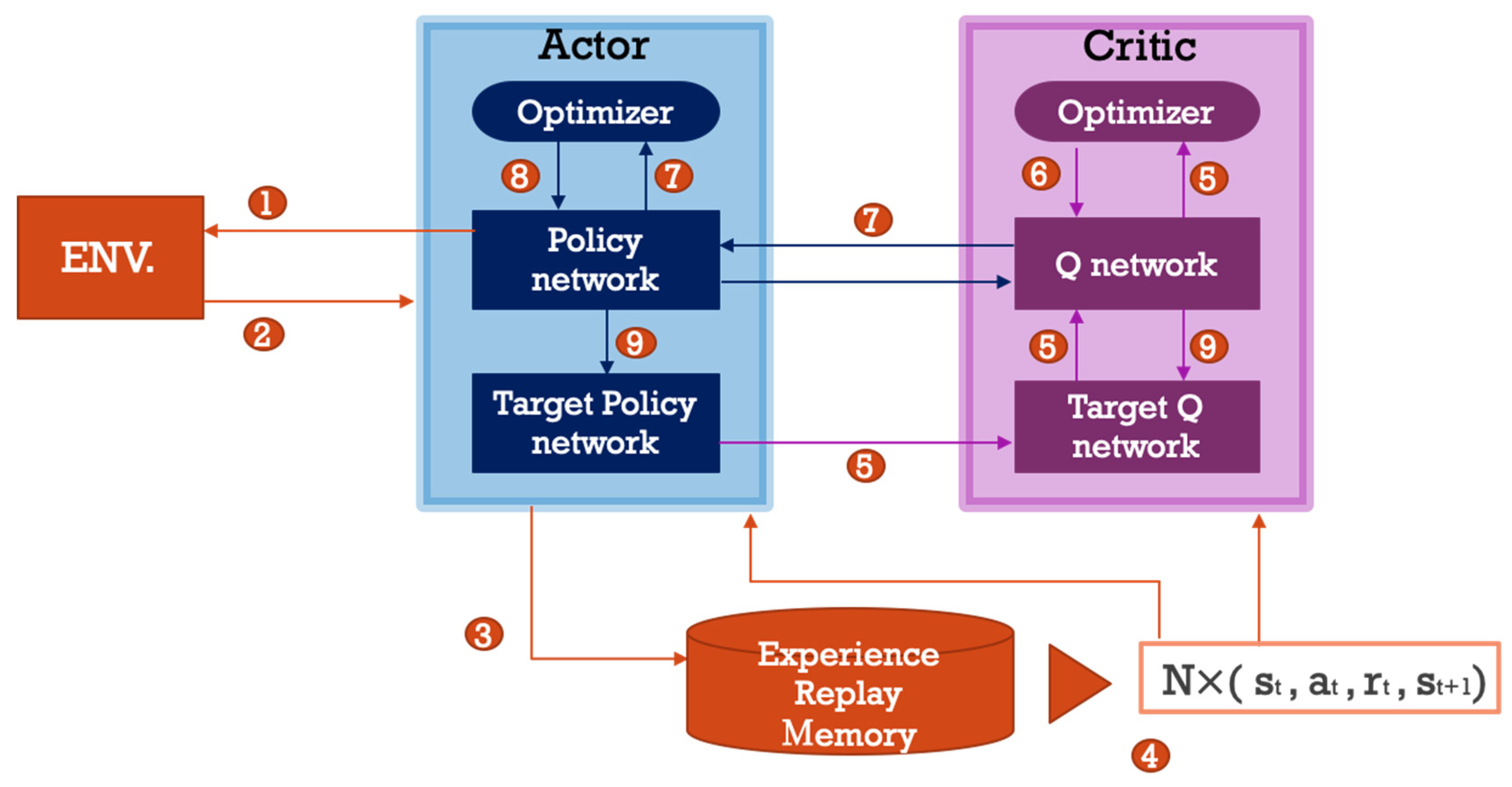
The DDPG algorithm, introduced in 2016 by Timothy P. Lillicrap et al. [22] from DeepMind, addresses reinforcement-learning challenges within continuous action spaces. This approach advances the Actor-Critic concept found in DPG while integrating the experience replay and target network aspects of DQN. Its architecture is illustrated in Figure 3.

The complete algorithm flow is shown in Figure 4. DDPG uses four neural networks, of which the Actor and Critic each have two networks, namely the Policy network, Target policy network, Q network, and Target q network. The update mechanism of the target network in DDPG differs slightly from that of DQN. In DQN, the target network is directly copied from the main network at fixed intervals. However, in DDPG, the target network is updated by employing a soft max approach; that is, the target network is updated gradually and converges slowly toward the respective main network. Its flow is as follows:

• Actor selects a A_t according to the behavior strategy as in Formula (8) and sends it to the agent to execute the A_t

  $$A_t=\mu \left(S_t|{\theta }^{\mu }\right)+N_t$$

  (8)

  In Formula (8), ${\theta }^{\mu }$ is a parameter in the Policy network, and the behavior policy is to obtain the value of $A_t$ from this random process according to the current policy $\mu$ and exploration noise $N_t$.
• Agent executes $A_t$, returns ${ R}_t$ and new state $S_{t+1}$.
• Actor stores this state transition process: ($A_t$, $S_t$, $R_t$, $S_{t+1}$) into the replay memory buffer as a data set for training the network.
• Randomly sample N conversion process data from the replay memory buffer as a mini-batch training data for the Policy network and Q network.
• Calculate the gradient of the Q network.

  $${{Loss}_{critic}=\frac{1}{N}\sum _i(y_i-Q(s_i,a_i|{\theta }^Q))}^2$$

  (9)

  $$y_i={\mathrm{r}}_i+\mathsf{\gamma }{Q}^{\prime }(S_{\mathrm{i}+1},{\mu }^{\prime }({\mathrm{S}}_{\mathrm{i}+1}\left|{\theta }^{{\mu }^{\prime }}\right)\left|{\theta }^{Q^{\prime }}\right)$$

  (10)

  In Formula (9), the loss function is used to update the critic network, where ${\theta }^Q$ is a parameter in the Q network.
  In Formula (10), $y_i$ is calculated by using ${\mu }^{\prime }$ of Target policy network and $Q^{\prime }$ of Target Q network so that the learning process of Q network parameters is more stable. Furthermore, $\mathsf{\gamma }$ is the reward discount factor; ${\theta }^{{\mu }^{\prime }}$ is the parameter of the Target policy network; and ${\theta }^{Q^{\prime }}$ is the parameter of the Target Q network.
• Update Q network.
• Calculate the policy gradient of the Policy network.

  $${{\nabla }_{\theta \mu } J\approx \frac{1}{N}\sum _i{\nabla }_{a}Q(s,a|{\theta }^Q)|}_{s=si,a=\mu \left(si\right)}{{\nabla }_{\theta \mu } \mu \left(s\right|{\theta }^{\mu }\left)\right|}_{si}$$

  (11)

  Formulas (2)–(15) employs policy gradient to update the Actor network. As a result, the parameter update of the Actors is enhanced to maximize the Q value.
• Update Policy network.
• Soft update target network.

  $${\theta }^{Q^{\prime }}\leftarrow \tau {\theta }^Q+\left(1+\tau \right){\theta }^{Q^{\prime }}$$

  (12)

  $${\theta }^{{\mu }^{\prime }} \leftarrow \tau {\theta }^{\mu }+\left(1+\tau \right){\theta }^{{\mu }^{\prime }}$$

  (13)

Furthermore, due to DDPG’s reliance on a deterministic strategy, its inherent exploration remains quite limited. Yet, exploration stands as a pivotal factor in training a proficient agent. To enhance its exploratory nature, noise $N_t$ is introduced for action exploration. When the agent selects an action, a certain level of noise is incorporated into the action produced by the Policy network (Actor). This noise could be random or derived from a specific distribution. The intention behind this addition is to elevate the potential for exploration capability, enabling the agent to traverse different action possibilities. This, in turn, facilitates a more comprehensive grasp of the environment’s dynamics and the optimal strategy.

3. Experimental Method

3.1. Experimental Purpose

To establish a comprehensive set of action strategies for guiding the gimbal’s target tracking, the initial step involves crafting a simulated environment through a game engine. This environment will subsequently undergo training via reinforcement learning. To align the simulation more closely with real-world conditions, the approach incorporates both UAV technology and YOLO technology for actual flight scenarios to capture flight images and observe the gimbal’s performance.

Initially, this setup involves deploying a UAV fitted with a camera gimbal, linked to the console via the drone’s flight control system. The camera records real-time UAV flight footage, which is transmitted to the console’s monitor. The subsequent step involves applying YOLO technology for target detection and localization. YOLO, a backbone comprising convolutional layers, pooling layers, and fully connected layers, facilitates real-time object detection [23]. In our context, YOLO scrutinizes the camera feed, discerns the target object, and acquires its location and category details. Upon detecting the target object, the UAV’s flight control system orchestrates gimbal actions in accordance with the target’s positional data. The gimbal’s role involves governing the camera’s pitch and yaw, ensuring the target object remains continuously within the camera gimbal’s field of view. Consequently, as the target shifts, the camera automatically adjusts its angle.

During live flight, the monitor provides insight into the camera gimbal’s perspective while the UAV is airborne. Meanwhile, it is possible to observe the gimbal’s movements and its alignment adjustments in response to the target’s position. This holistic approach contributes to refining the simulation’s resemblance to real-world scenarios.

3.2. Simulated Environment

Unity stands as a cross-platform 2D/3D game engine crafted by Unity Technologies, a game software development company in San Francisco, CA, USA.

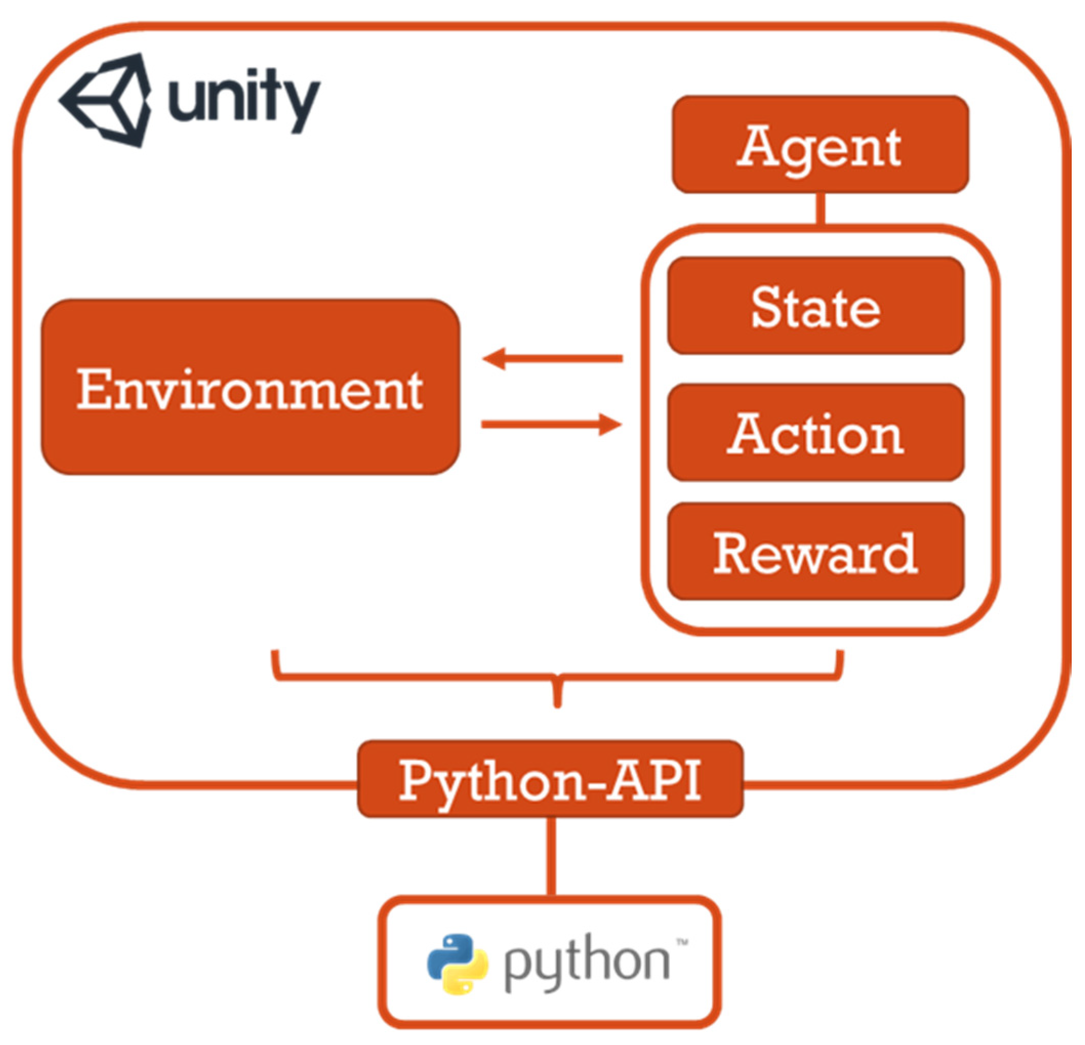
The simulation environment is developed using Unity 2022.3.19f1 version. Within Unity, an open-source toolkit named Unity Machine Learning Agent (ML-Agent) is available for embedding machine learning in Unity development. This toolkit furnishes developers with a user-friendly yet potent framework for training intelligent agents, empowering them to learn and autonomously make decisions. Moreover, the Unity Python API is supplied, serving as an interface to communicate with and control Unity via Python. This setup permits the program creations in Python to manipulate the Unity environment. Consequently, a simulation environment is created through Unity, as shown in Figure 5. Python and reinforcement learning converge via the Python API. The simulation environment’s state is adopted as input, and PyTorch-crafted neural networks facilitate the training process.

3.3. State Design

As detailed in Section 3.1, the initial step involves deploying a UAV equipped with a camera gimbal for real flight to capture the gimbal’s screens during actual flight. On the screen, there is an H-shaped icon with a diameter of 110 cm, and a black dot, generated using OpenCV, marks the center (Figure 6).

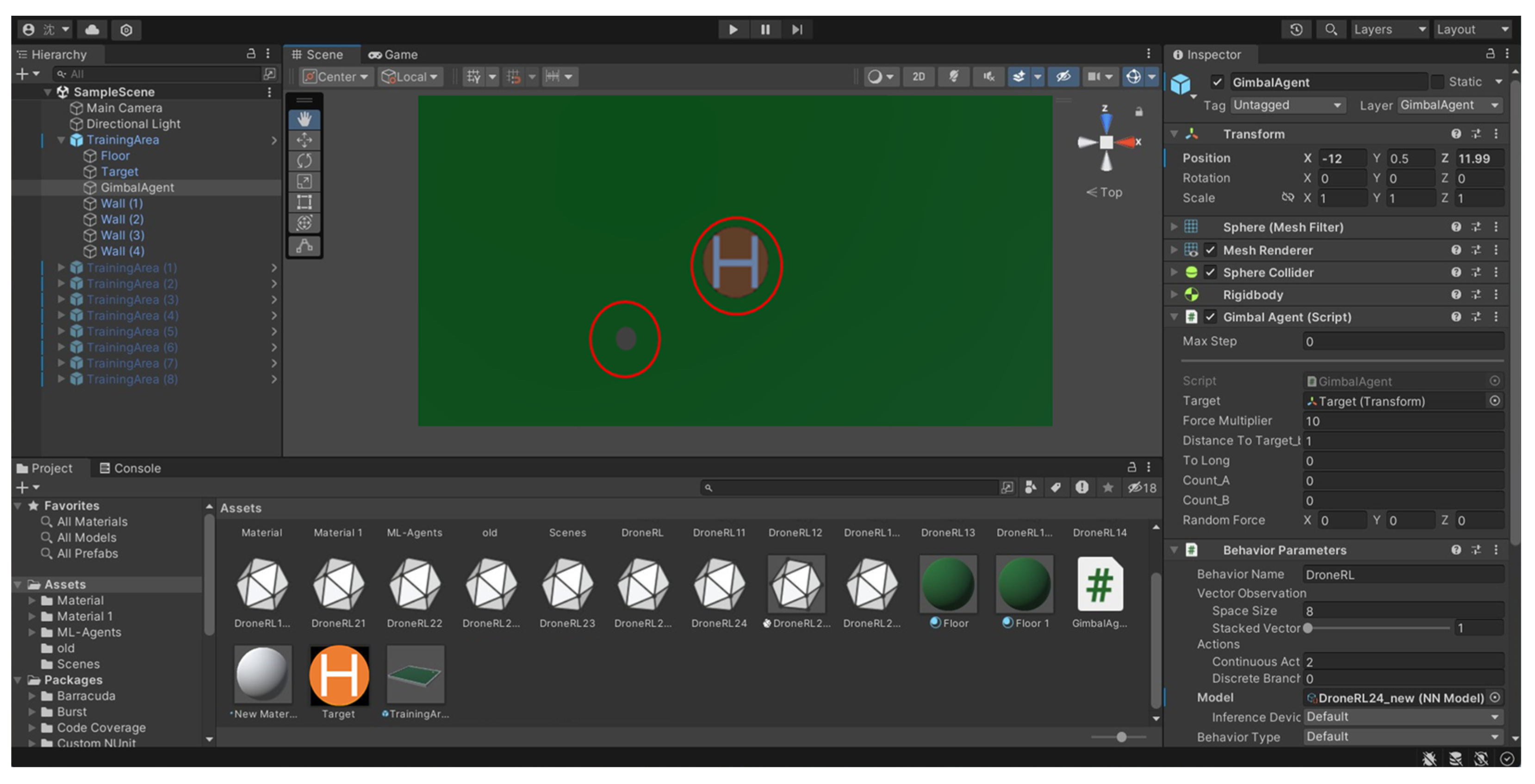
Hence, this study employs the genuine flight screen as a reference and establishes the screen size at 960 × 480, defining the agent’s feasible movement range. Both the target and the agent are positioned within this defined range. The initial state initializes the target object (referred to as H) at the screen center. Simultaneously, the agent (represented as a black point within the simulated environment) is generated at the predetermined initial position, as depicted in Figure 7. To enhance the environment’s alignment with actual conditions, the simulated UAV experiences disturbances from environmental wind during flight. Consequently, when the agent tracks the target, the target’s position introduces random deviations around its initial location. This emulation mirrors the target’s response after the UAV encounters imagery affected by crosswinds.

3.4. Action Design

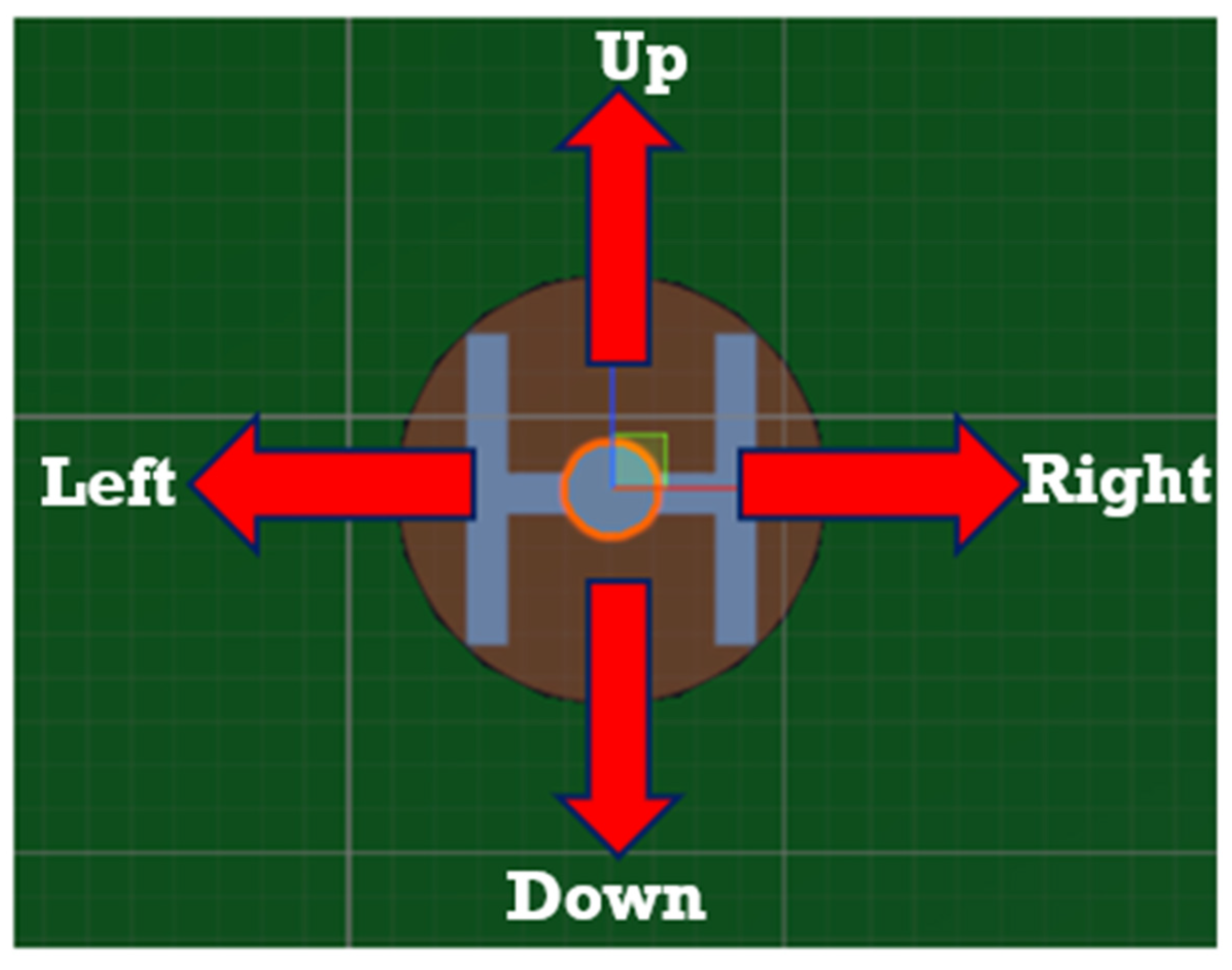
In reinforcement learning, to interact with the environment and obtain feedback, an agent must choose an action from an action space to perform. Therefore, this study expects to train an agent through reinforcement learning, which can track and locate the target. According to the movement of the gimbal observed during the actual flight and the operating instructions of the program, four actions can be conducted by the agent, namely up, down, left, and right, as shown in Figure 8. Among them, forward is defined as the action when the pitch angle of the gimbal is adjusted from −110° to +70°; backward is defined as the action when the pitch angle of the gimbal is adjusted from +70° to −110°; and left and right are defined as the gimbal yaw angle completing a $\pm$360° rotation, as shown in Figure 9.

Table 1. Agent action set.

Type	Simulation	Real World
Action 1	Up	pitch (−110° to +70°)
Action 2	Down	pitch (+70° to −110°)
Action 3	Left	yaw (−360°)
Action 4	Right	yaw (+360°)

shows the agent’s actions and the corresponding Pan–Tilt–Zoom (PTZ) actions represented by it.

3.5. Reward Design

In reinforcement learning, the design of rewards holds immense significance, as rewards constitute a pivotal element in agent learning. Thoughtfully crafted rewards can guide the agent to learn behaviors aligned with expectations, whereas improper designs may lead the agent to acquire policies that deviate from the intended objective. During agent–environment interaction, rewards can be bestowed based on the fulfillment of reward conditions. These rewards might manifest as positive or negative feedback.

The objective behind the four actions outlined in Section 3.4 is to enable the agent (depicted as a black dot) to track and locate the target (marked as point H). Thus, when the agent executes an action that successfully brings it over the target, a positive reward of $+10$ is granted, while the agent’s actions that lead it away from the goal or beyond the defined range invoke negative penalty scores. Furthermore, in real-flight tracking and control, traditional point-to-point methods necessitate recalculations at each step, preventing the selection of the most efficient path. To mitigate this, a slight penalty is introduced into the reward mechanism. This entails attaching a penalty to every agent’s action. This mechanism prompts the agent to meticulously consider each action, subsequently learning to minimize its actions and devise an action strategy that yields the highest reward. Hence, the devised reward and penalty mechanism is summarized in

Table 2. Reward and mechanism table.

Perform Actions	Reward Points
Successfully tracked target	+10
Out of range	−5
Each execution step	−1
Reduced distance to target	+5
Increased distance to target	−5

.

4. Experimental Results

This section will commence with an in-depth analysis of the experimental simulation results. Reinforcement learning unfolds through the interplay of action execution, reward acquisition, and state transition. Ultimately, the training objective is to cultivate a repertoire of action strategies that offer maximal rewards. Consequently, the training progress can be grasped most intuitively by observing the accumulation of acquired rewards. First, the cumulative rewards obtained from post-training are recorded within the dataset, as illustrated in

Table 3. Reward accumulation.

Perform Actions	Reward
Epoch 1	−10
Epoch 2	−22
Epoch 3	4
Epoch 4	−6
Epoch 5	11
⋮	⋮
Epoch 80	30
Epoch 81	28
Epoch 82	31
⋮	⋮
Epoch 199	32
Epoch 200	30

. Then, Python’s data processing and visualization tools are employed to transform the stored reward accumulation data into graphical representations, as depicted in Figure 10. Finally, this visual presentation serves to enhance the clarity in discerning the trend and alterations in reward accumulation, further highlighting the impact of the training process.

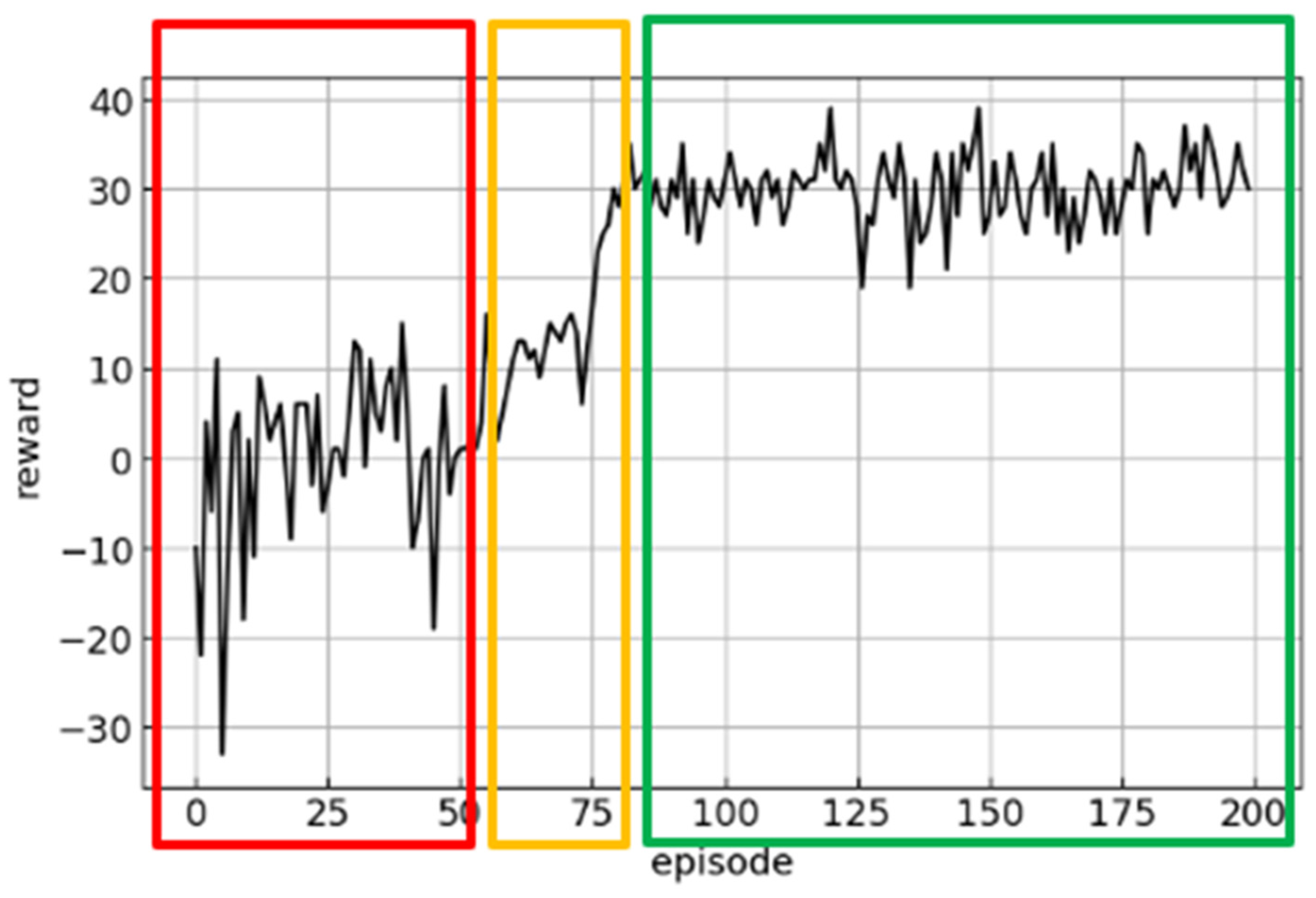
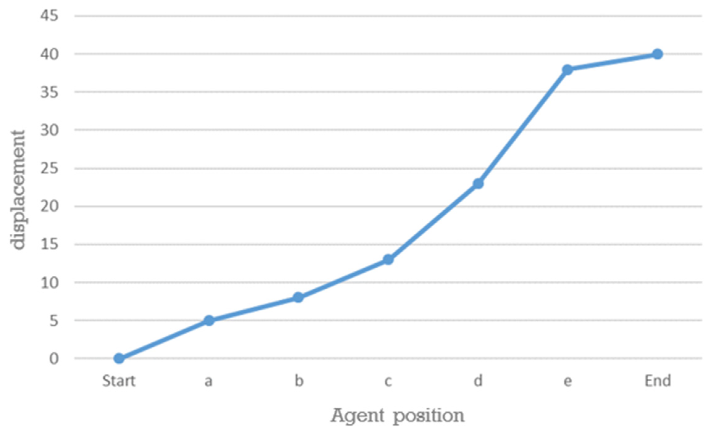
Upon examining Figure 11, insights can be obtained from the reward curve describing the agent’s learning process in three distinct phases, as illustrated in Figure 10. These stages encompass the exploration phase (framed in red), the gradual stabilization phase (framed in orange), and the eventual state of stable convergence (framed in green).

4.1. Exploration Phase

From Figure 12, it becomes evident that within the initial 50 rounds of training, the agent’s reward accumulation experiences notable instability, with the reward value fluctuating within the range of −33–15. This signifies that during this phase, the agent has yet to ascertain an effective strategy for accomplishing the task objective; instead, it engages in diverse actions within the exploration space. The training screen further underscores this exploration phase, as depicted in Figure 13. Here, the agent may explore various directions, represented by $a_1$, $b_1$, and $c_1$ arrows indicating movement, to assess their impact on attaining bettering rewards. This transiently erratic reward accumulation aligns with expectations, considering that the agent needs to understand how to optimize rewards through its interactions with the environment.

4.2. Gradual Stabilization Phase

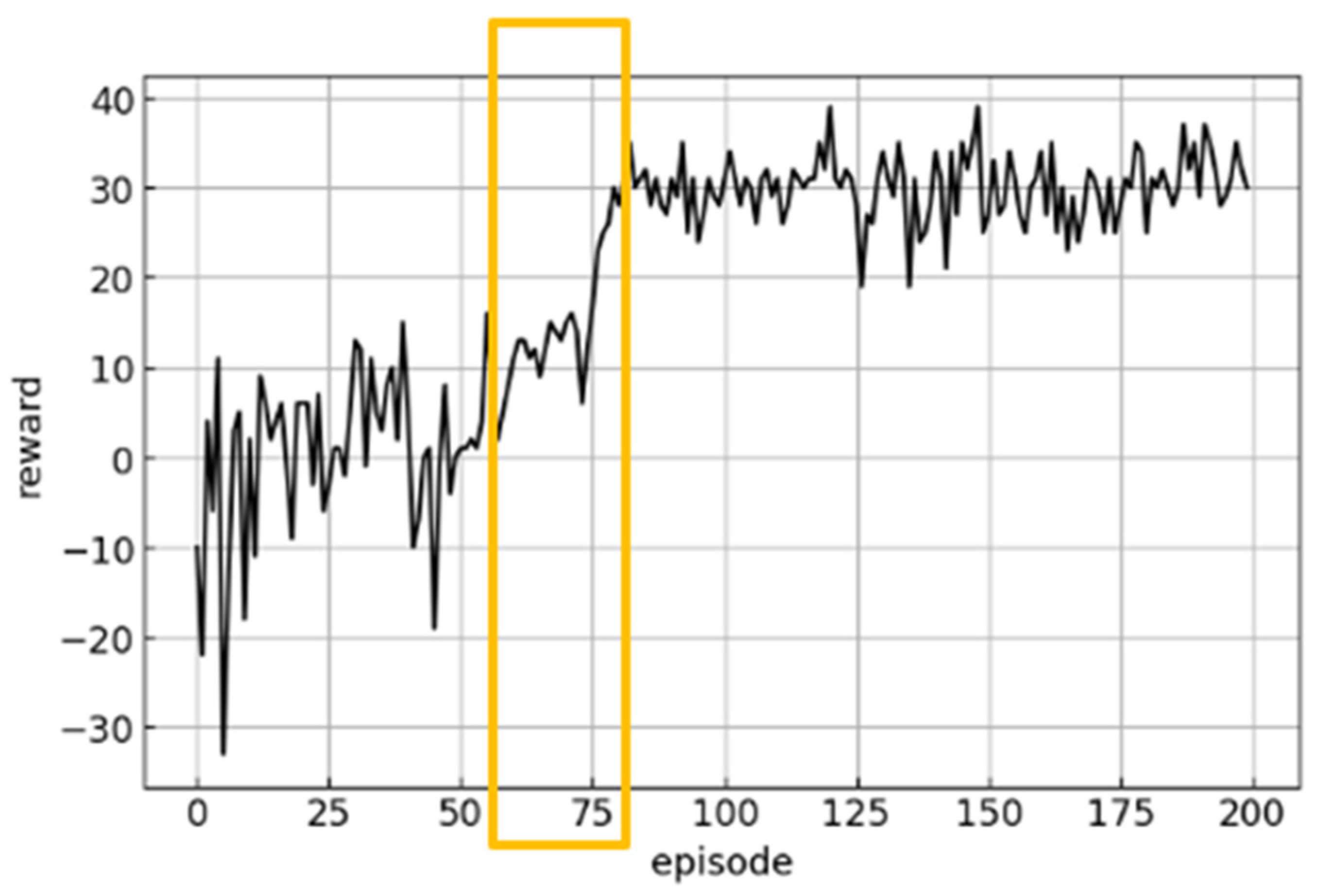
Turning to Figure 14, the interval from 50 to 80 rounds in training reveals a gradual rise in reward accumulation, with reward values spanning 1–30. This indicates that following the exploratory phase early in training, the agent begins to link actions with elevated rewards, thereby mastering the task of tracking the target. Progress in this training span underscores the enhancement in the agent’s capacity to learn and comprehend the task of object tracking. Continued training is anticipated to yield ongoing increases in reward accumulation, with the agent’s strategy and action choices becoming more refined and efficient.

Additionally, scrutiny of the training screen (Figure 15) showcases that the agent, at this juncture, has acquired a vital strategy: approaching the target to heighten reward acquisition. This underscores the agent’s ability to learn, adapt, and extract advantageous insights from the environment to facilitate appropriate actions. However, within the strategy assimilated by the agent at this phase, an essential aspect remains absent: how to track the target through the most efficient trajectory.

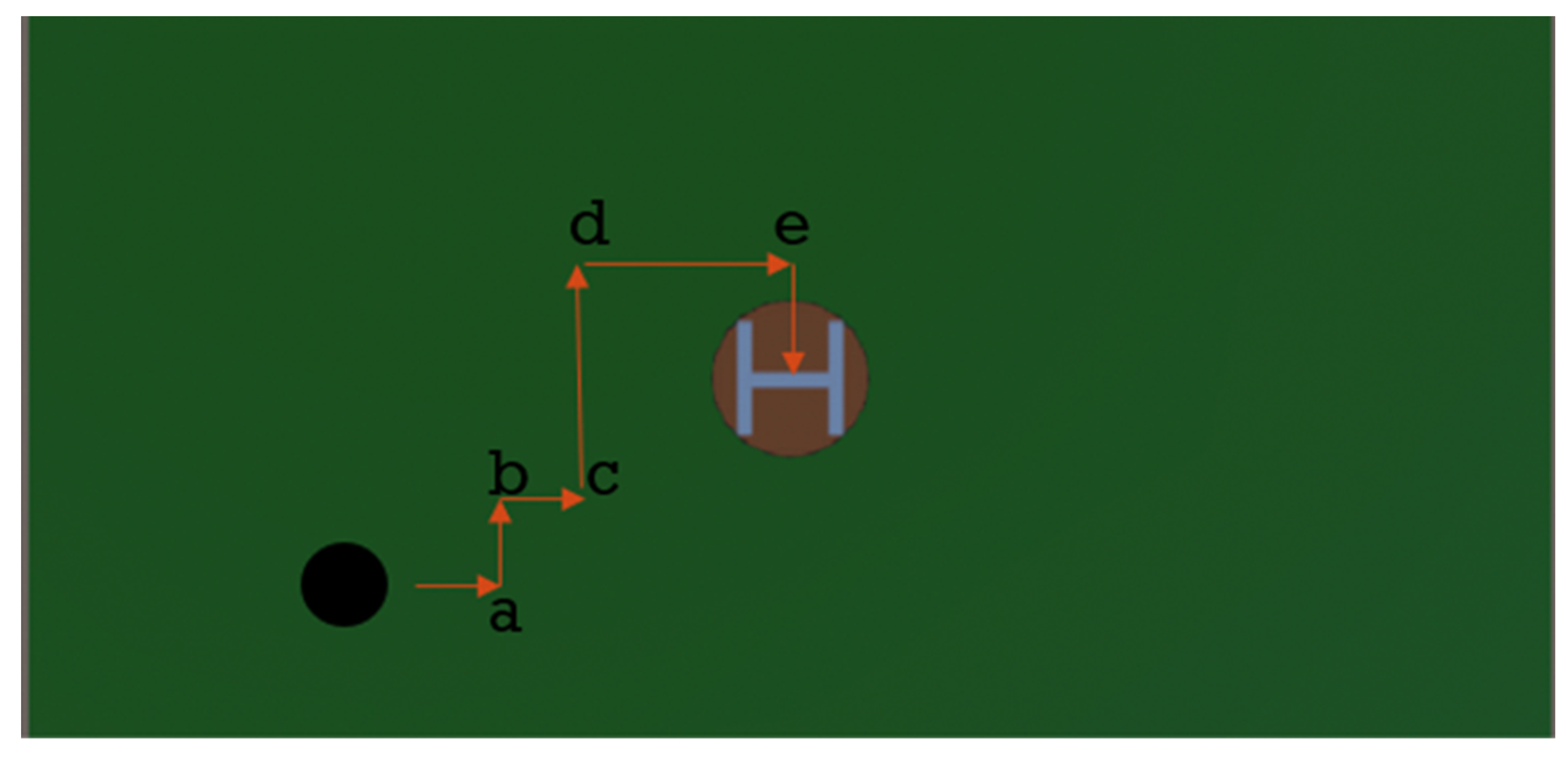
Simultaneously, by linking the positions of moving points, this process can be quantified as a displacement graph, as depicted in Figure 16. This graphical representation provides a clearer perspective of the distance the agent must traverse from the initial bottom left position (−25, −15) to the centering target position during the learning process. Moreover, it offers insight into the total number of steps required to accomplish the task of tracking the target.

4.3. Stable Convergence Phase

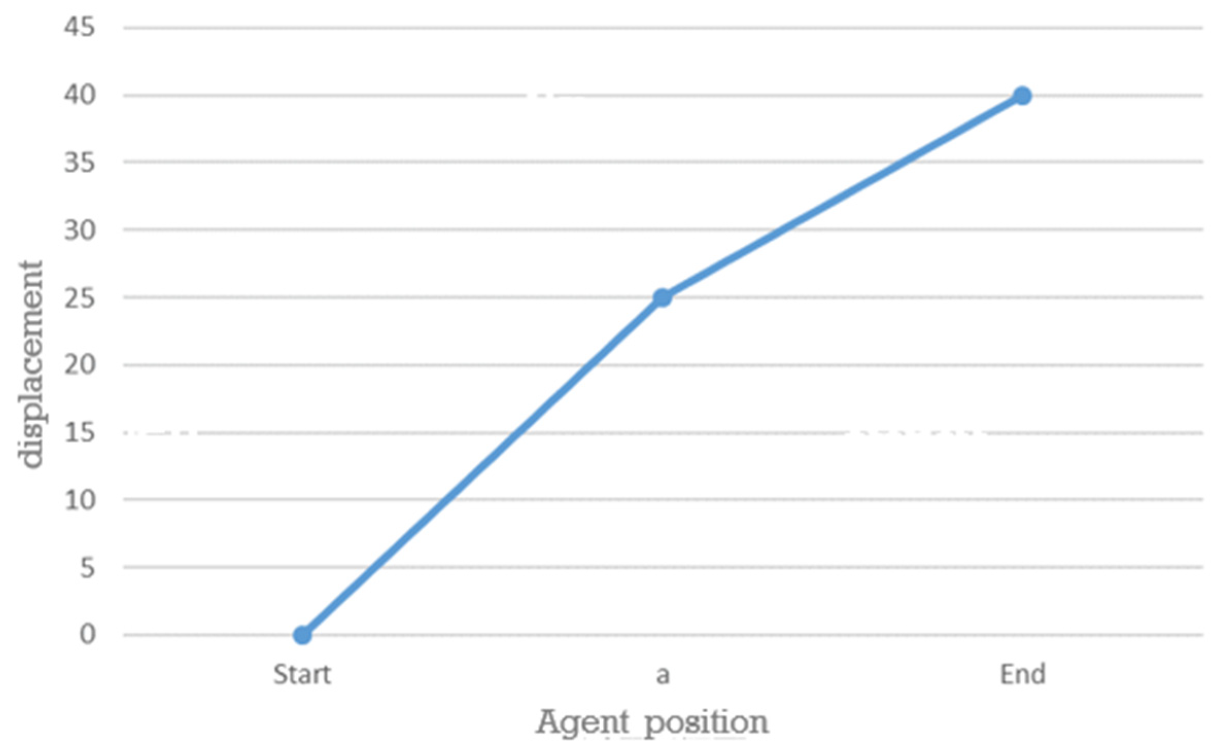
As training progresses to the 80 rounds (Figure 17), reward accumulation has gradually stabilized and converged. Within the range of 19–39, reward values exhibit consistency, and the magnitude of fluctuations has diminished from 33 to 20. This indicates that the agent has incrementally uncovered a more optimal strategy throughout the learning process, enabling it to secure consistent rewards in its interactions with the environment. The stability and convergence of these rewards signify that as the agent amasses experience and advances in learning, it progressively discerns improved action choices, relentlessly striving to attain higher rewards.

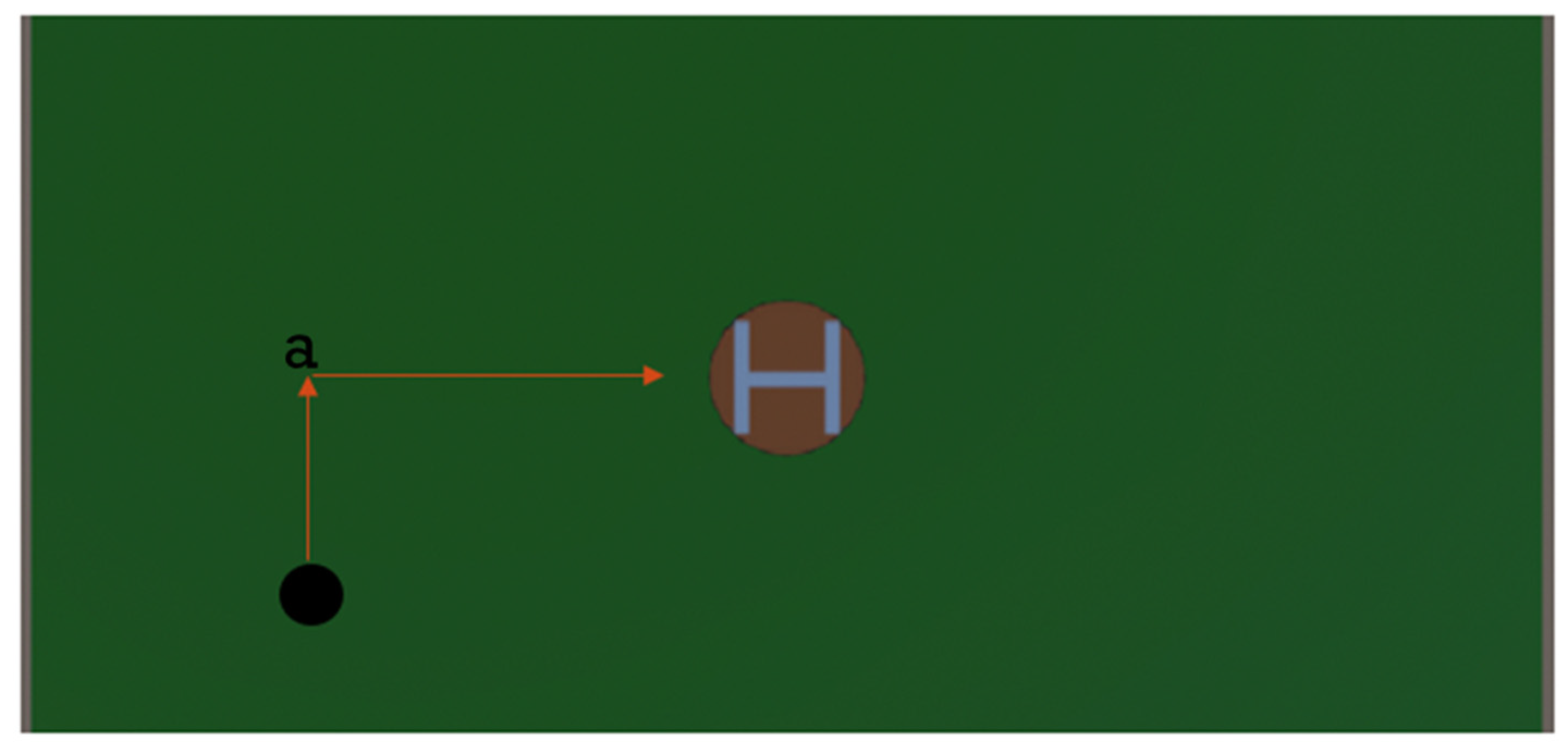
Through analysis of the displacement curve (refer to Figure 18), it is evident that the agent’s grasp extends beyond merely tracking the target as the primary objective—specifically, moving from the initial position (−25, −15) to the target position. Through accumulated experience, the agent covers a total distance of 40 units. Simultaneously, it learns to track along the most efficient path, completing the task in a mere two steps, as shown in Figure 19.

4.4. Introduction of External Interference

In the later stages of the experiment, to better emulate real-flight conditions, random external disturbances were introduced to simulate crosswinds during flight. To replicate authentic crosswind scenarios, these external disturbances were generated randomly across the X, Y, and Z axes. The magnitude of the external disturbance force ranged from $-$5 to 5 Newtons, as depicted in Figure 4, Figure 5, Figure 6, Figure 7, Figure 8, Figure 9, Figure 10, Figure 11 and Figure 12. The intended wind direction after setup is illustrated in Figure 20.

Figure 21 demonstrates a decrease in the average cumulative reward to some extent, accompanied by heightened volatility. This outcome arises because the agent conducts more actions to counterbalance errors due to crosswind influences, indirectly leading to increased penalties and affecting cumulative rewards. Nevertheless, convergence is sustained from epoch 100 rounds, indicating the agent’s sustained effectiveness in tracking.

Notably, despite heightened external disturbances posing challenges, the agent continues to adapt and optimize its action strategy to achieve improved tracking outcomes. This underscores reinforcement learning’s adaptability and resilience in response to environmental fluctuations. Through continuous learning and optimization, the agent can effectively overcome external interferences and accomplish its desired tracking objective.

4.5. Performance of Camea Visual Tracking for an Object of Square Motion by PID and RL Controllers

This experiment investigates the performance of camera gimbal tracking on a square moving object. The control performance of the camera under different environmental scenarios (models) is tested. The performance of engaging the target by PID controller and reinforcement learning controller will be compared. Therefore, in reinforcement learning, three different environment models will be constructed and trained with no wind interference and continuous wind interference.

4.5.1. Training Performance of Camea Visual Tracking an Object in Square Positioning

In the training environment, the camera gimbal remains fixed in the same position, while the initial position of the tracking target position is randomly generated within the region of 30 m². This training strategy is for the yaw and pitch control ability for camera surveillance. The training loop ends when the camera gimbal successfully tracks (engages) the target or when the target moves out of the frame of the training environment. The next training loop will continue with a new episode.

Following are the reward settings for the reinforcement training, consisting of four reward mechanism modes. The first mode, engaging the target during tracking, yields +10 points, while moving out of the environment frame incurs a penalty of −10 points. In the second mode, engaging the target during tracking yields +10 points, moving out of the environment frame incurs a penalty of −10 points, and each additional searching step results in a penalty of −0.1. In the third mode, engaging the target during tracking yields +10 points, moving out of the environment frame incurs a penalty of −10 points, each additional searching step results in a penalty of −0.1, and getting closer to the target adds a bonus of +0.2. In the fourth mode, engaging the target during tracking yields +10 points, moving out of the environment frame incurs a penalty of −10 points, each additional searching step results in a penalty of −0.1, getting closer to the target adds a bonus of +0.2, and getting farther away the target incurs a penalty of −0.2. These four reward–penalty modes were constructed as listed in

Table 4. Four modes of reward setting for tracking a target with a square motion.

Type	Action	Reward
Mode 1	Engaging	+10
	Moving out	−10
Mode 2	Engaging	+10
	Moving out	−10
	Each additional searching step	−0.1
Mode 3	Engaging	+10
	Moving out	−10
	Each additional searching step	−0.1
	Closer to the target	+0.2
Mode 4	Engaging	+10
	Moving out	−10
	Each additional searching step	−0.1
	Closer to the target	+0.2
	Farther away the target	−0.2

. This experiment constructs eight reinforcement learning controller (RLc) models for different environments and four reward mechanisms, as shown in

Table 5. Reinforcement learning control models with different environments and reward types.

RL Model Name	Environment	Reward Type
RLc 1	no wind interference	Mode 1
RLc 2		Mode 2
RLc 3		Mode 3
RLc 4		Mode 4
RLc 5	continuous wind interference	Mode 1
RLc 6		Mode 2
RLc 7		Mode 3
RLc 8		Mode 4

.

In the reward–penalty plot of training, two training environments comprised of no wind interference and continuous wind interference are compared with four reward modes, as presented in Figure 22. As shown in Figure 22, the trend of the curve in the RLc 5 curve (Red) indicates that around 500 K (0.5 × 10⁶) steps, the training period is comparatively chaotic. This is attributed to the influence of the continuous wind environment and the reward setting of the training mechanism. This plot indicates that the learning progress required a significant amount of exploration time, thereby leading to the inability of phenomena to converge during the training’s transient behavior. This is due to a poorly designed reward mechanism, causing the training process to enter an endless loop where the reward seems to fail to converge to 10 points. Compared with other curves in Figure 23, it can be observed that the RLc5 curve (Red) exhibits a significantly higher total step in the interval of 500 K episodes.

During the testing phase, the dynamic response for tracking a target with the reinforcement learning control for the camera gimbal will be evaluated. The target will execute square motion trajectories with a spacing of 30 m², as shown in Figure 24. Experiments were conducted under three interference environments: single interference like an impulse input to the camera at some specific time, continuous interference (random excitation), and mixed interference (single plus continuous excitation). The interference to the camera gimbal may be caused by the wind or structure vibration of the UAV. Each interference condition will be implemented.

4.5.2. Testing Performance of Camea Visual Tracking an Object in Square Positioning

First, in the single-interference environment, the target executes a path along the four sides. The camera gimbal experiences external interference in the middle of each path segment. In this experiment test, the PID controller and eight models of reinforcement learning controllers are compared. Experimental results show that the PID controller outperforms the eight types of RLc models in dynamic tracking, as shown in Figure 25 and Figure 26. As depicted in the plot, the tracking trajectory deviated away from the path due to the injecting interference. The total tracking error of the PID control is 2755.2 m. It is the lowest among all curves, as shown in

Table 6. Total error of the PID and RLc controllers disturbed by single-interference environment.

Type	X Total Error (m)	Y Total Error (m)	Total Error (m)
PID controller	1376.527	1378.641	2755.168
RLc 1s	1639.447	1771.039	3410.486
RLc 2s	1515.326	1659.746	3175.072
RLc 3s	1757.004	1947.581	3704.585
RLc 4s	1863.846	1641.37	3505.216
RLc 5s	2436.504	2419.995	4856.499
RLc 6s	1817.888	2150.425	3968.313
RLc 7s	1987.844	2248.281	4236.125
RLc 8s	2473.454	2182.709	4656.163

. Nevertheless, the stability of the PID and RL controllers still holds, though the disturbance was applied to the camera gimbal.

Secondly, when the continuous-interference environment is applied, the results show that RLc 7 demonstrates superior dynamic tracking, as shown in Figure 27 and Figure 28. The total error of 4005.712 is the lowest among all curves, as shown in

Table 7. The total error of the PID and RLc controllers disturbed by continuous-interference environment.

Type	X Total Error	Y Total Error	Total Error
PID controller	2571.234	2689.52	5260.754
RLc 1c	2067.507	2531.231	4598.738
RLc 2c	1920.636	2314.86	4235.496
RLc 3c	2140.647	2583.775	4724.422
RLc 4c	2211.103	2148.11	4359.213
RLc 5c	1837.215	2730.256	4567.471
RLc 6c	1728.02	2375.396	4103.416
RLc 7c	1557.849	2447.863	4005.712
RLc 8c	2040.935	2232.779	4273.714

. It is also observed that the PID controller exhibited inferior control performance compared to RLc when the continuous interference was tested. Since the conventional PID controller is good in the linear- and model-based dynamic plant, the disturbance rejecting for the continuous interference is not as good as the nonlinear-based RLc controller. This indicates that using reinforcement-learning control is better suited for dealing with the outside environment when the UAV is operated. The best tracking result made by RLc 7 may be caused by the total reward design that is positive as 0.1. Then, RLc 7 tries to execute the bettering disturbance rejection based on the incentive of the positive reward design.

Thirdly, in the mixed-interference environment test, experimental results show that RLc 6 in reinforcement learning demonstrates superior dynamic tracking, as shown in Figure 29 and Figure 30. The total error of 4335.915 is the lowest among all curves, as shown in

Table 8. Total error in the mixed-interference environment.

Type	X Total Error	Y Total Error	Total Error
PID controller	2824.23	3049.346	5873.576
RLc 1m	2182.383	2873.302	5055.685
RLc 2m	2027.009	2491.253	4518.262
RLc 3m	2248.814	2873.627	5122.441
RLc 4m	2419.873	2500.419	4920.292
RLc 5m	2098.563	3113.346	5211.909
RLc 6m	1705.526	2630.389	4335.915
RLc 7m	1636.336	2715.977	4352.313
RLc 8m	2148.323	2646.956	4795.279

. Similarly, the performance of the PID controller is still inferior to reinforcement learning. In reinforcement learning, it is observed that both RLc 2 and RLc 6 effectively overcome environments with continuous interference. In the single disturbance training dataset, both RLc 2 and RLc 6 resulted in less error, as shown in Table 6. Thus, the test result reveals that the impulse of the disturbance at some specific time dominates the performance of the RL controller. RLc 2 and RLc 6 seem to do the memory for a pre-determined disturbance rejection.

In terms of the X and Y axes error data, the Y-axis error is mostly greater than the X-axis error. The training data contain more datasets in the X-direction than in the Y-direction, thus causing an imbalance in the XY axes errors.

4.6. Training and Test of RL Controller by Transfer Learning

The training environments for the above camera tracking object experiments include no interference and continuous interference. Next, based on the above testing results, the new type of transfer learning is deployed based on the conclusion of using the reward modes 2, 3, and 4. By comparing the error from the aforementioned results (Table 6, Table 7 and Table 8), the best weights were selected individually from the no interference and continuous interference training environment. They are specifically conducted via RLc 2, RLc 4, RLc 6, and RLc 7.

This transfer-learning training reward mechanism will be adjusted here. Engaging the target during tracking yields +2 points, while touching (engaging) continuously for 500 times yields +10 points, with a condition of continuous touching (engaging) error less than 0.1 m. This design policy is to fulfill the requirement that the camera should capture the object continuously by several frames. During the surveillance, ensuring target is the key issue. We placed a restricted condition for 500 times. This new rule will be incorporated into the rewards of Mode 2, Mode 3, and Mode 4, and then updating them to Mode 5, Mode 6, and Mode 7, as shown in

Table 9. The transfer-learning reward setting for tracking a target with a square motion.

Type	Action	Reward
Mode 5	Engaging continuously 500 times	+10
	Engaging	+2
	Moving out	−10
	Each additional searching step	−0.1
Mode 6	Engaging continuously 500 times	+10
	Engaging	+2
	Moving out	−10
	Each additional searching step	−0.1
	Closer to the target	+0.2
Mode 7	Engaging continuously 500 times	+10
	Engaging	+2
	Moving out	−10
	Each additional searching step	−0.1
	Closer to the target	+0.2
	Farther away the target	−0.2

. This reward–penalty mechanism was not utilized in the Section 4.5 environment because it tends to allow the RL algorithm to give up, go back to the searching area, and then move out of the frame. Such a learning process leads to premature termination, thus rendering the reinforcement-learning training ineffective.

In this training phase, through transfer learning, we can update four new models, RLc 9, RLc 10, RLc 11, and RLc 12, as shown in

Table 10. The transfer-learning, reinforcement-learning models with a square motion.

RL Model Name	Environment	Reward Type
RLc 9	no wind interference	Mode 5
RLc 10		Mode 7
RLc 11	continuous wind interference	Mode 5
RLc 12		Mode 6

. At this phase, in order to increase the aim of applying the stabilized reinforcement-learning tracking capability, the epoch training parameters are adjusted to 7,500,000 iterations (as shown in Figure 31).

First, in the transfer-learning single-interference environment, experimental results show that the PID controller outperforms the reinforcement-learning models after transfer learning in dynamic tracking, as shown in Figure 32 and Figure 33. The PID total error of 2755.168 is the lowest among all curves, as shown in

Table 11. Total error in the transfer learning in single-interference environment.

Type	X Total Error (m)	Y Total Error (m)	Total Error (m)
PID controller	1376.527	1378.641	2755.168
RLc 9s	1843.629	1628.196	3471.825
RLc 10s	1616.028	1943.649	3559.677
RLc 11s	1540.768	1919.177	3459.945
RLc 12s	2036.984	2400.906	4437.89

. It can be inferred that transfer learning does not effectively improve in the single-interference environment. This may be the reason that the impulse disturbance injection may cause RLc to search the historical sharp but arbitrary error compensation. However, the steady-state-like transfer learning at this time frame tries to return to the initial transient-like transfer learning. Such a state, action, and reward function will reshuffle again and then degrade the tracking error performance.

Secondly, in the transfer-learning continuous-interference environment, experimental results show that RLc 11c demonstrates superior dynamic tracking, as shown in Figure 34 and Figure 35. The total error of 3335.779 is the lowest among all curves, as shown in

Table 12. Total error in the transfer-learning continuous-interference environment.

Type	X Total Error (m)	Y Total Error (m)	Total Error (m)
PID controller	2571.234	2689.52	5260.754
RLc 9c	2223.737	2221.629	4445.366
RLc 10c	1931.952	2583.501	4515.453
RLc 11c	1539.821	1795.958	3335.779
RLc 12c	1450.878	2479.654	3930.532

.

Thirdly, in the transfer-learning mixed-interference environment, experimental results show that RLc 11 in reinforcement learning demonstrates superior dynamic tracking, as shown in Figure 36 and Figure 37. The total error of 3551.858 is the lowest among all curves, as shown in

Table 13. Total error in the transfer-learning mixed-interference environment.

Type	X Total Error (m)	Y Total Error (m)	Total Error (m)
PID controller	2824.23	3049.346	5873.576
RLc 9m	2342	2494.434	4836.434
RLc 10m	2045.529	2774.131	4819.66
RLc 11m	1581.889	1969.969	3551.858
RLc 12m	1548.453	2758.587	4307.04

. Compared to other models, RLc 11 exhibits improved dynamic response after transfer learning in both continuous and mixed environments.

5. Conclusions

This study utilizes Unity to establish a simulation environment for controlling a gimbal’s target tracking. It trains a set of action strategies through reinforcement learning, facilitating accurate target tracking while minimizing unnecessary movements and enhancing tracking efficiency. Training within a simulated environment offers convenience, cost savings, and diverse environmental conditions for comprehensive training and testing scenarios. Thus, the contributions of this study and some comments can be summarized as follows:

• With reinforcement learning, a set of action strategies is trained to enable precise target tracking by the gimbal. Through exploration and feedback, the agent gains insights from its interactions with the environment. Training outcomes reveal a stable convergence of reward values within the range of 19–35, accompanied by a decrease in shock amplitude from the initial value of 33 to 16. In essence, adopting a learned strategy leads to the consistent attainment of high rewards for accomplishing the tracking task.
• Reinforcement learning effectively curtails extraneous movements during tracking, thereby enhancing tracking efficiency. Conventional tracking methods often involve continuous distance calculations between the target and the gimbal, leading to unnecessary movements and energy wastage. However, analyzing the displacement curve reveals that only essential actions are taken—specifically, a two-step tracking based on the distance between the agent and the target. This approach reduces unnecessary movements, increases tracking efficiency, and conserves energy.
• Training within a simulated environment simplifies learning and reduces training expenses. This environment offers a range of scenarios, simulating diverse potential conditions for training and testing agents. This enhances the flexibility and control of the learning process while lowering risks and real-world expenses. Additionally, training in this simulated environment enables the more efficient optimization of action strategies, leading to improved outcomes in real-world applications.
• In the experiment of camera gimbal tracking a target, applying a conventional PID controller can outperform the RLc models when the disturbance injection along the path tracking is simple. However, with continuous wind interference and mixed vibrational-interference environments, the reinforcement learning models outperformed the PID controllers. This indicates using reinforcement learning control is better suitable for dealing with the undetermined and complex outside environment when the UAV’s camera gimbal is operated.
• The methodology of transfer learning can be utilized to develop RL control. Designated reward mechanisms can enhance the adaptability of the RL models. Simulation results consolidate that the performance of the RL models is better than the original model before transfer learning and the conventional PID controller. This demonstrates the significance of the reward–penalty mechanisms on the RL.
• The YOLO’s failure may be due to several reasons and can be rescued by the following procedures. First, when the shutdown of the YOLO program occurs, the UAV can hover and restart the YOLO program. Secondly, when visual recognition causes abnormality in the environment, the YOLO confidence threshold should be remotely adjusted. An adaptive threshold adjustment technique will be implemented and enable the engaged recognition of the target. Thirdly, when the UAV cannot resolve the object detection while hovering, searching for nearby suitable landing points and controlling the UAVs to land at the landing point [24] should be the next steps.

References

1. Mnih, V.; Kavukcuoglu, K.; Silver, D.; Graves, A.; Antonoglou, I.; Wierstra, D.; Riedmiller, M. Playing Atari with Deep Reinforcement Learning. arXiv 2013, arXiv:1312.5602. [Google Scholar]
2. Silver, D.; Lever, G.; Heess, N.; Degris, T.; Wierstra, D.; Riedmiller, M. Deterministic Policy Gradient Algorithms. In Proceedings of the 31st International Conference on Machine Learning (ICML), Beijing, China, 21–26 June 2014; Volume 32, pp. 387–395. [Google Scholar]
3. Mnih, V.; Kavukcuoglu, K.; Silver, D.; Rusu, A.A.; Veness, J.; Bellemare, M.G.; Graves, A.; Riedmiller, M.; Fidjeland, A.K.; Ostrovski, G.; et al. Human-level control through deep reinforcement learning. Nature 2015, 518, 529–533. [Google Scholar] [CrossRef] [PubMed]
4. Mnih, V.; Badia, A.P.; Mirza, M.; Graves, A.; Lillicrap, T.; Harley, T.; Silver, D.; Kavukcuoglu, K. Asynchronous Methods for Deep Reinforcement Learning. arXiv 2016, arXiv:1602.01783. [Google Scholar]
5. Bellemare, M.G.; Dabney, W.; Munos, R. A Distributional Perspective on Reinforcement Learning. In Proceedings of the 34th International Conference on Machine Learning (ICML), Sydney, Australia, 6–11 August 2017; Volume 70, pp. 449–458. [Google Scholar]
6. Fortunato, M.; Azar, M.G.; Piot, B.; Menick, J.; Osband, I.; Graves, A.; Mnih, V.; Munos, R.; Hassabis, D.; Pietquin, O.; et al. Noisy Networks for Exploration. arXiv 2017, arXiv:1706.10295. [Google Scholar]
7. Hessel, M.; Modayil, J.; van Hasselt, H.; Schaul, T.; Ostrovski, G.; Dabney, W.; Horgan, D.; Piot, B.; Azar, M.; Silver, D. Rainbow: Combining Improvements in Deep Reinforcement Learning. In Proceedings of the Thirty-Second AAAI Conference on Artificial Intelligence, New Orleans, LA, USA, 2–7 February 2018; Volume 32. [Google Scholar] [CrossRef]
8. Fernandez-Gauna, B.; Ansoategui, I.; Etxeberria-Agiriano, I.; Graña, M. Reinforcement learning of ball screw feed drive controllers. Eng. Appl. Artif. Intell. 2014, 30, 107–117. [Google Scholar] [CrossRef]
9. Huang, Y.C.; Chan, Y.C. Manipulating XXY Planar Platform Positioning Accuracy by Computer Vision Based on Reinforcement Learning. Sensors 2023, 23, 3027. [Google Scholar] [CrossRef] [PubMed]
10. Kalashnikov, D.; Irpan, A.; Pastor, P.; Ibarz, J.; Herzog, A.; Jang, E.; Quillen, D.; Holly, E.; Kalakrishnan, M.; Vanhoucke, V.; et al. QT-Opt: Scalable Deep Reinforcement Learning for Vision-Based Robotic Manipulation. arXiv 2018, arXiv:1806.10293. [Google Scholar]
11. Faust, A.; Oslund, K.; Ramirez, O.; Francis, A.; Tapia, L.; Fiser, M.; Davidson, J. PRM-RL: Long-range Robotic Navigation Tasks by Combining Reinforcement Learning and Sampling-based Planning. arXiv 2017, arXiv:1710.03937. [Google Scholar]
12. Tzeng, E.J.; Chen, S.C.; Chen, J.L.; Roche, A.E.; Chen, J.L. Robotic limb gait-tracking using deep-q-network. In Proceedings of the Euspen’s 21st International Conference & Exhibition, Copenhagen, Denmark, 7–10 June 2021; Available online: https://www.euspen.eu/knowledge-base/ICE21248.pdf (accessed on 28 July 2023).
13. Yi, L. Lane Change of Vehicles Based on DQN. In Proceedings of the 2020 5th International Conference on Information Science, Computer Technology and Transportation (ISCTT), Shenyang, China, 13–15 November 2020; pp. 593–597. [Google Scholar]
14. Reddy, D.R.; Chella, C.; Teja, K.B.R.; Baby, H.R.; Kodali, P. Autonomous Vehicle Based on Deep Q-Learning and YOLOv3 with Data Augmentation. In Proceedings of the 2021 International Conference on Communication, Control and Information Sciences (ICCISc), Idukki, India, 16–18 June 2021; Volume 1, pp. 1–7. [Google Scholar]
15. Lin, Y.C.; Nguyen, H.L.T.; Yang, J.F.; Chiou, H.J. A reinforcement learning backstepping-based control design for a full vehicle active Macpherson suspension system. IET Control. Theory Appl. 2022, 16, 1417–1430. [Google Scholar] [CrossRef]
16. Huang, X.; Luo, W.; Liu, J. Attitude Control of Fixed-wing UAV Based on DDQN. In Proceedings of the 2019 Chinese Automation Congress (CAC), Hangzhou, China, 22–24 November 2019; pp. 4722–4726. [Google Scholar]
17. Pham, H.X.; La, H.M.; Feil-Seifer, D.; Van Nguyen, L. Reinforcement Learning for Autonomous UAV Navigation Using Function Approximation. In Proceedings of the 2018 IEEE International Symposium on Safety, Security, and Rescue Robotics (SSRR), Philadelphia, PA, USA, 6–8 August 2018; pp. 1–6. [Google Scholar]
18. Lee, H.; Yun, W.J.; Jung, S.; Kim, J.H.; Kim, J. DDPG-based Deep Reinforcement Learning for Loitering Munition Mobility Control: Algorithm Design and Visualization. In Proceedings of the 2022 IEEE VTS Asia Pacific Wireless Communications Symposium (APWCS), Seoul, Republic of Korea, 24–26 August 2022; pp. 112–116. [Google Scholar]
19. Taghibakhshi, A.; Ogden, N.; West, M. Local Navigation and Docking of an Autonomous Robot Mower Using Reinforcement Learning and Computer Vision. In Proceedings of the 2021 13th International Conference on Computer and Automation Engineering (ICCAE), Melbourne, Australia, 20–22 March 2021; pp. 10–14. [Google Scholar]
20. Mashhouri, S.; Rahmati, M.; Borhani, Y.; Najafi, E. Reinforcement Learning based Sequential Controller for Mobile Robots with Obstacle Avoidance. In Proceedings of the 2022 8th International Conference on Control, Instrumentation and Automation (ICCIA), Tehran, Iran, 2–3 March 2022; pp. 1–5. [Google Scholar]
21. Sutton, R.S.; Barto, A.G. Reinforcement Learning: An Introduction, 2nd ed.; MIT Press: Cambridge, MA, USA, 2018. [Google Scholar]
22. Lillicrap, T.P.; Hunt, J.J.; Pritzel, A.; Heess, N.; Erez, T.; Tassa, Y.; Silver, D.; Wierstra, D. Continuous control with deep reinforcement learning. arXiv 2016, arXiv:1509.02971. [Google Scholar]
23. Redmon, J.; Divvala, S.; Girshick, R.; Farhadi, A. You Only Look Once: Unified, Real-Time Object Detection. arXiv 2015, arXiv:1506.02640. [Google Scholar]
24. Ma, M.Y.; Shen, S.E.; Huang, Y.C. Enhancing UAV Visual Landing Recognition with YOLO’s Object Detection by Onboard Edge Computing. Sensors 2023, 23, 8999. [Google Scholar] [CrossRef] [PubMed]
Figure 1. Reinforcement learning architecture diagram.
Drones 08 00174 g001
Figure 2. Markov decision process model [21].
Drones 08 00174 g002
Figure 3. Deep Deterministic Policy Gradient architecture diagram.
Drones 08 00174 g003
Figure 4. Deep Deterministic Policy Gradient algorithm flow chart.
Drones 08 00174 g004
Figure 5. Simulation system architecture.
Drones 08 00174 g005
Figure 6. Screen obtained during the actual flight. (a) 10 m above the ground (b) 5 m above the ground. The black dot in (a,b) indicates the center of the camera screen while the green box is the Yolo’s identified visual screen.
Drones 08 00174 g006
Figure 7. Simulated PTZ screen.
Drones 08 00174 g007
Figure 8. Camera gimbal’s action diagram for object detection.
Drones 08 00174 g008
Figure 9. The diagram of actual drone’s gimble movement (a) up (b) down (c) left (d) right.
Drones 08 00174 g009
Figure 10. Cumulative reward graph.
Drones 08 00174 g010
Figure 11. Three learning stages.
Drones 08 00174 g011
Figure 12. Exploration phase (Red).
Drones 08 00174 g012
Figure 13. Pretraining (action exploration).
Drones 08 00174 g013
Figure 14. Gradual stabilization phase (yellow).
Drones 08 00174 g014
Figure 15. Mid-training (closer to target to increase reward acquisition).
Drones 08 00174 g015
Figure 16. Displacement curve 1.
Drones 08 00174 g016
Figure 17. Stable convergence phase (green).
Drones 08 00174 g017
Figure 18. Displacement Curve 2.
Drones 08 00174 g018
Figure 19. Late phase of training (acting on the most efficient path).
Drones 08 00174 g019
Figure 20. Intended wind direction (the red arrow indicates wind direction).
Drones 08 00174 g020
Figure 21. Cumulative rewards after the introduction of external interference.
Drones 08 00174 g021
Figure 22. Plot of the UAV’s camera gimbal rewards with episodes when different environments are simulated.
Drones 08 00174 g022
Figure 23. The total number of training steps in each episode.
Drones 08 00174 g023
Figure 24. The trajectory (blue) of the target moves along a square of 30 m2 and with a windy interference (red).
Drones 08 00174 g024
Figure 25. X-axis dynamic tracking response due to single-interference environment.
Drones 08 00174 g025
Figure 26. Y-axis dynamic tracking response due to single-interference environment.
Drones 08 00174 g026
Figure 27. X-axis dynamic tracking response in the continuous-interference environment.
Drones 08 00174 g027
Figure 28. Y-axis dynamic tracking response in the continuous-interference environment.
Drones 08 00174 g028
Figure 29. X-axis dynamic tracking response in the mixed-interference environment.
Drones 08 00174 g029
Figure 30. Y-axis dynamic tracking response in the mixed-interference environment.
Drones 08 00174 g030
Figure 31. Illustration for stabilized initial transfer-learning weight in Figure 22 followed by four stabilized new transfer-learning RL controllers.
Drones 08 00174 g031
Figure 32. X-axis dynamic response in the transfer-learning single-interference environment.
Drones 08 00174 g032
Figure 33. Y-axis dynamic response in the transfer-learning single-interference environment.
Drones 08 00174 g033
Figure 34. X-axis dynamic response in the transfer-learning continuous-interference environment.
Drones 08 00174 g034
Figure 35. Y-axis dynamic response in the transfer-learning continuous-interference environment.
Drones 08 00174 g035
Figure 36. X-axis dynamic response in the transfer-learning mixed-interference environment.
Drones 08 00174 g036
Figure 37. Y-axis dynamic response in the transfer-learning mixed-interference environment.
Drones 08 00174 g037