Article

A Drone’s 3D Localization and Load Mapping Based on QR Codes for Load Management

1
Department of Artificial Intelligence, Dongguk University, Seoul 04620, Republic of Korea
2
Department of Computer Science and Engineering, Dongguk University, Seoul 04620, Republic of Korea
*
Author to whom correspondence should be addressed.
Drones 2024, 8(4), 130; https://doi.org/10.3390/drones8040130
Submission received: 27 February 2024 / Revised: 20 March 2024 / Accepted: 25 March 2024 / Published: 29 March 2024

Abstract

:
The ongoing expansion of the Fourth Industrial Revolution has led to a diversification of drone applications. Among them, this paper focuses on the critical technology required for load management using drones. Generally, when using autonomous drones, global positioning system (GPS) receivers attached to the drones are used to determine the drone’s position. However, GPS integrated into commercially available drones have an error margin on the order of several meters. This paper, proposes a method that uses fixed-size quick response (QR) codes to maintain the error of drone 3D localization within a specific range and enable accurate mapping. In the drone’s 3D localization experiment, the errors were maintained within a specific range, with average errors ranging from approximately 0 to 3 cm, showing minimal differences. During the mapping experiment, the average error between the actual and estimated positions of the QR codes was consistently around 0 to 3 cm.

1. Introduction

In this study, we propose technologies for drone logistics management. The key to inventory management using drones is accurate positioning of the drones and identifying the location of the load. Currently, drone positioning technology generally relies on global positioning system (GPS), but it has an error of several meters in commercial drones [1]. To solve this problem, recently developed drones equipped with GPS technology such as RTK-GPS [2] and CDGPS [3], with an error of only a few centimeters, are used to solve this problem. However, the drawback of these GPS-equipped drones is their high cost.
In addition, recent studies have proposed using radio frequency identification(RFID) for load management to identify the location of the load [4,5], but false identification or non-identification of tags depending on the signal sensitivity of the RFID reader, and more importantly, RFID tags cannot generate a load map.
Therefore, in this study, we propose a method using a conventional commercial drone with a basic camera and quick response (QR) code attached to the floor to achieve more precise positioning and generate a load map. The proposed method estimates the drone position through the geometric relationship between the camera and QR code without the need for expensive sensor equipment and further identifies occurs the position of the load QR code based on the estimated position of the drone to generate a load map.
Although this study is similar to simultaneous localization and mapping (SLAM) research in terms of estimating location and a map creating, it cannot use the keyword “simultaneous” because, in conventional SLAM, the location estimation and map creation are not separate tasks. Instead, the trajectory is executed based on the previous map created in the location estimation process, and the previous map is updated based on the current estimated location. Then, a map is created from sensor data measured at the current actual location, and the error is corrected by comparing the two maps. However, in this paper, the estimation is based on QR codes, and only real-time QR code data in the video is used, not the previously acquired sensor information. Therefore, instead of comparing the similarity between the created map and the actual map, this paper compares the actual position coordinates of the drone with the estimated position coordinates. Additionally, the accuracy of load map creation is verified by examining how accurate the measured position of the load QR codes is.
The overall structure of this paper is as follows. Section 2 deals with related works. Section 2.1 is titled Simultaneous Localization And Mapping, Section 2.2 is titled Structure of QR Code and Section 2.3 is titled Camera Pinhole Model. Section 3 deals with the proposed method. Section 3.1 is titled Assumption for Proposed Method, Section 3.2 is titled Proposed Drone 3D Localization Algorithm, and Section 3.3 is titled Load Mapping Algorithm. Section 4 deals with experimental results in which simulator-based experiments (Section 4.1), real-world experiments using drones (Section 4.2), and experiments conducted with GPS attached to actual drones (Section 4.3) were conducted to verify the performance of the proposed method.

2. Related Works

2.1. Simultaneous Localization and Mapping

The SLAM technology is essential for all robots and refers to the process in which a robot detects its surrounding environment using sensors while identifying its position and creating a map [6,7,8,9,10,11,12]. When feature points are input through the sensors to perceive the surrounding situation, the robot identifies its position and posture using these feature points. Afterward, the estimated position and input sensor data are fused to redefine the existing feature points, and if the feature points are not in their previous location, they are adjusted to update the map.
The SLAM method exists in various types depending on the robot form and the sensor. Furthermore, SLAM can be categorized into lidar SLAM [13,14,15,16,17,18], visual SLAM [19,20,21,22,23], and others based on the type of sensor, and can also be divided into feature-based SLAM [15,16], fraph-based SLAM [17,18], etc., based on the method of data processing.
Lidar SLAM refers to the process of using lidar sensors for SLAM. There are various approaches to processing data in lidar SLAM. One of the most representative approaches is lidar odometry and mapping in real-time SLAM [15], which solves the problem of optimizing numerous variables using two separate algorithms. The first algorithm measures the speed of the lidar, and the second algorithm precisely matches and updates the set of sensor data (point cloud) obtained from the lidar sensor. This approach results in high-quality mapping, but because the lidar sensor data occur in real-time while the robot is moving, errors may occur if the sensor data and estimated robot position information do not match. A closed loop must be created to resolve this problem. In addition, LOAM SLAM is also a feature-based SLAM and requires a powerful embedded device to calculate many feature points. Moreover, LeGO-LOAM SLAM [16] was developed to reduce the high computational load of LOAM SLAM. This method reduces computation while improving safety by applying the loop back algorithm. However, it does not address the need for a closed loop, which is a feature of LOAM SLAM. The HDL Graph SLAM method [17,18] is another example of 3D lidar SLAM that uses the normal distribution transformation scan matching method to estimate the robot’s driving distance and loop detection in graph-based SLAM.
Visual SLAM refers to SLAM that uses cameras as sensors. Various types of cameras exist (e.g., monocular cameras, stereo cameras, RGB-D cameras, etc.); thus, many SLAM algorithms use them. Visual SLAM is classified as feature-based SLAM because it works based on various feature points detected in camera images. One advantage of visual SLAM is that it is cheaper than lidar SLAM because it uses cameras. However, due to the nature of the cameras, noise can occur in the image data, such as lighting conditions and object texture, which can result in errors and cumulative errors in creating a map using feature points. Filtering and optimization techniques are methods used to solve these problems by filtering and optimizing feature points. Examples include the Kalman [21,22] and particle [22,23] filters. The Kalman filter maps feature points in the image to landmarks using Gaussian distribution and estimates the position to keep the error of feature points within a specific range. However, if the error of feature points continues to accumulate, the map creation itself can eventually fail. Therefore, existing SLAM algorithms are unsuitable for use in load management. Additionally, machine learning-based localization methods have also been proposed. For instance, there are machine learning and deep learning-based 3D indoor visible light positioning methods [24]. However, this approach is also unsuitable for our problem because additional environmental modifications are required such as ceiling LEDs.

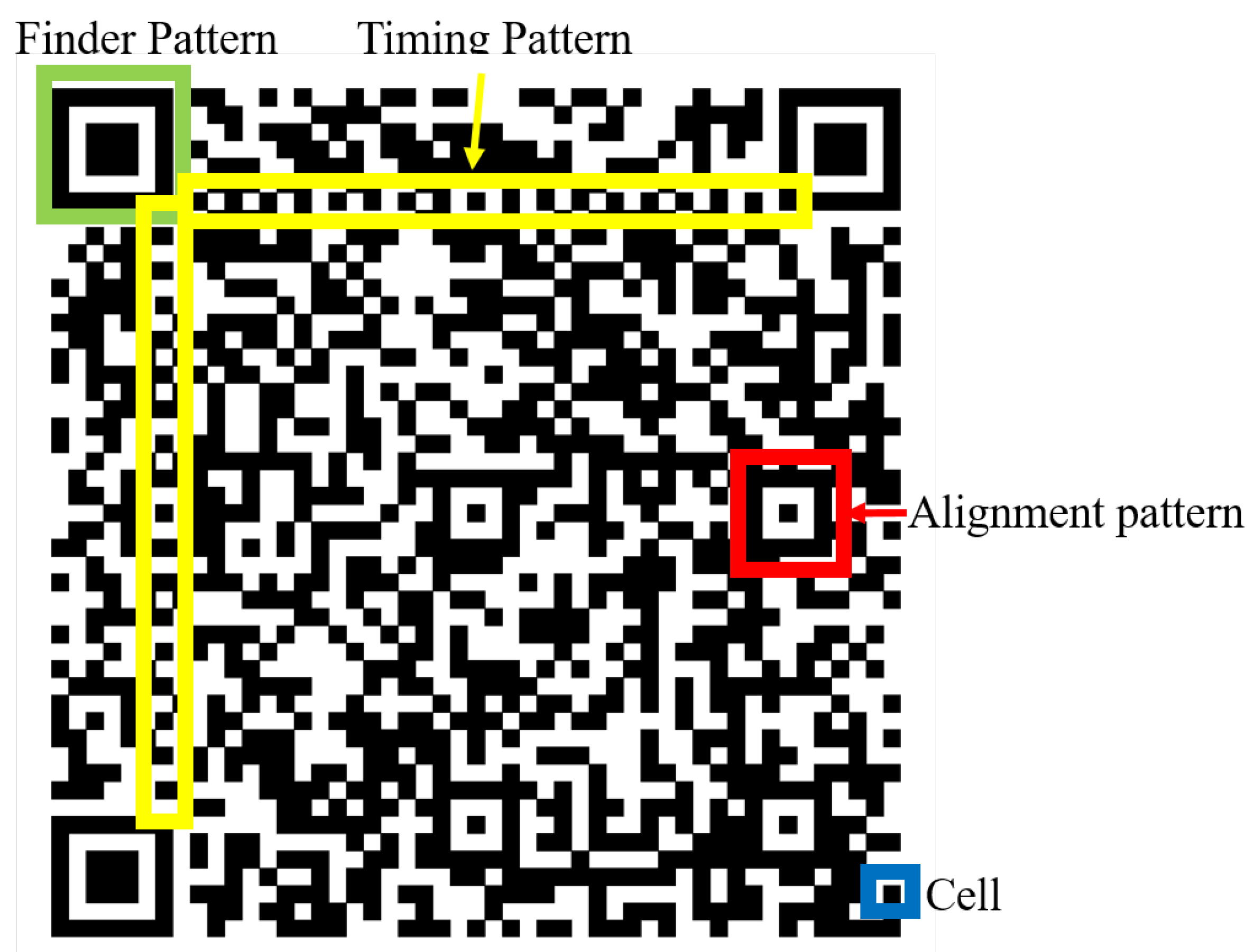
2.2. Structure of QR Code

The algorithm proposed in this paper is based on QR codes. Therefore, this section, explains the basic structure of QR codes, as illustrated in Figure 1 [25,26]. The finder pattern of the QR code is a pattern for detecting the position of the QR code on the photograph. By finding this pattern, the position of the code can be quickly identified, and high-speed reading is possible. The alignment pattern is an auxiliary pattern used to determine the cell location when it deviates due to distortion. The size of the QR code determines these patterns. The timing pattern alternates between black and red along the finder pattern. The coordinates of the cells are estimated using the timing pattern.

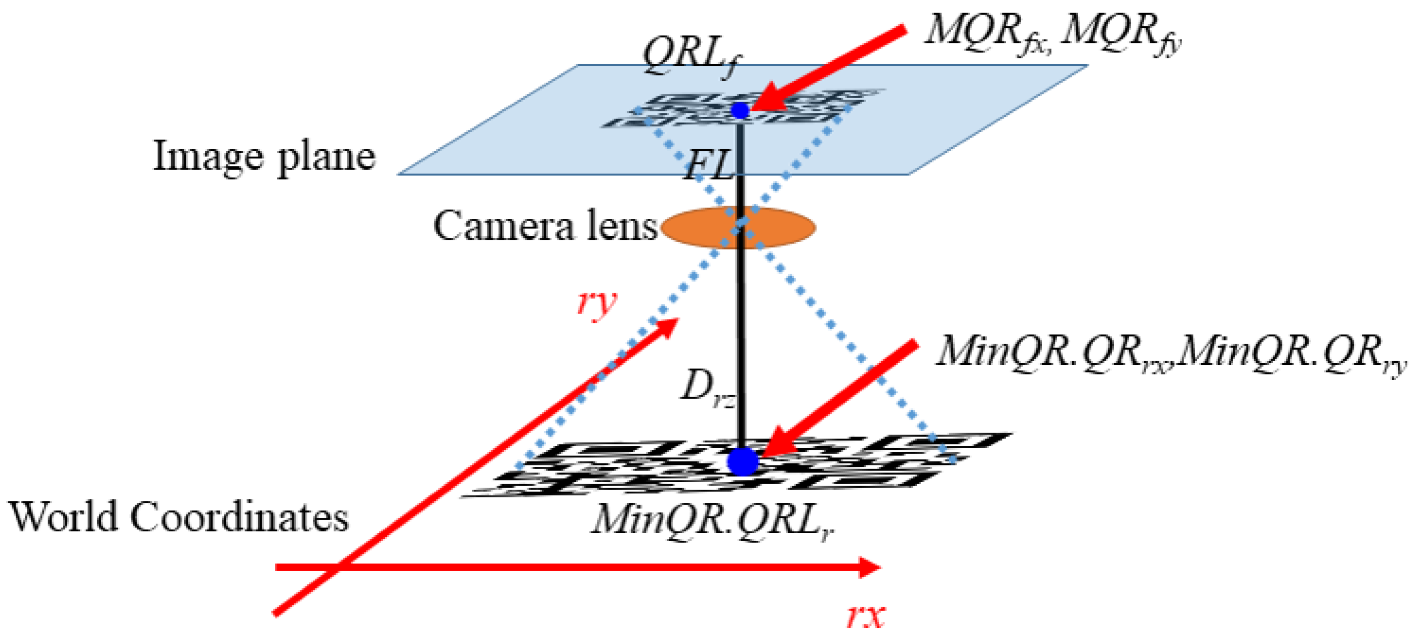
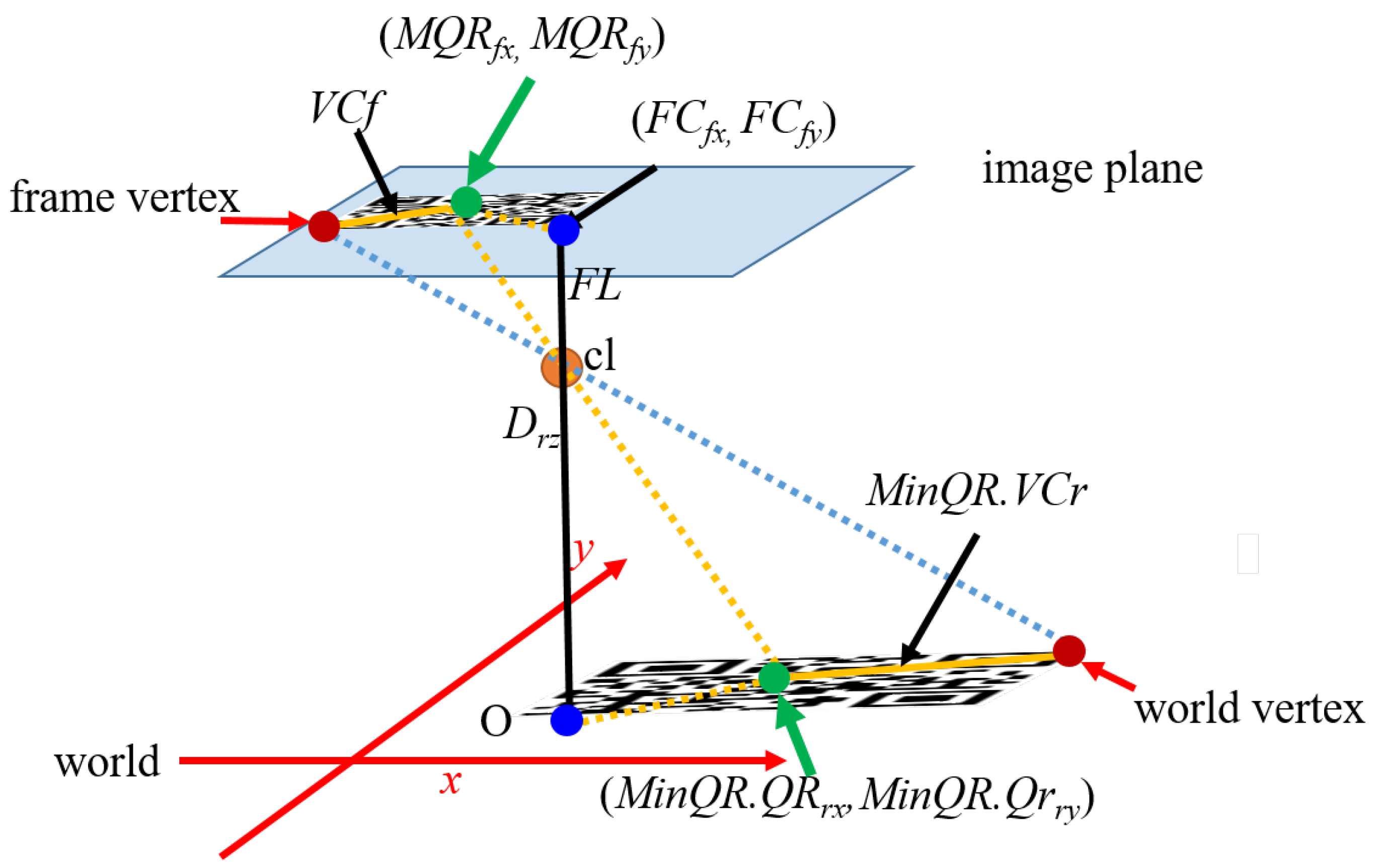
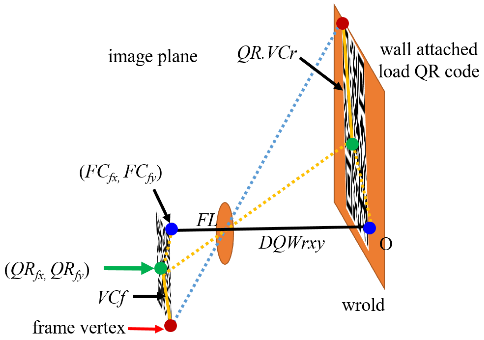
2.3. Camera Pinhole Model
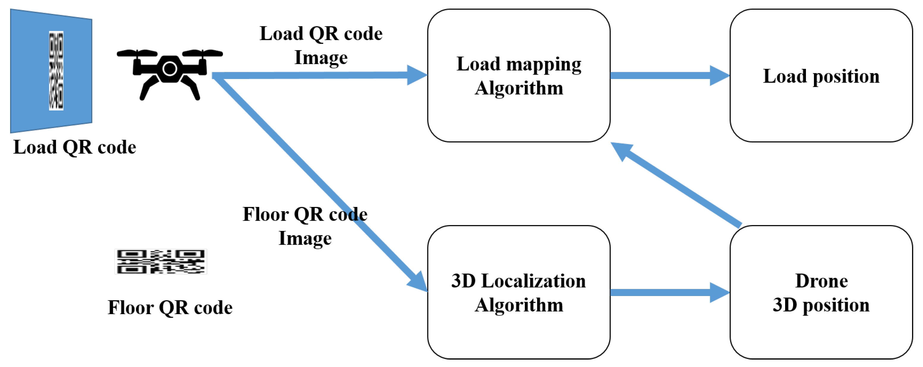
Before explaining the details of the algorithm, the camera pinhole model that forms the basis for the mathematical modeling of the algorithm is explained. The camera pinhole model [27] refers to the structure where the actual object passes through a small hole (pinhole) and forms an image on the camera image sensor, as depicted in Figure 2. Assuming that I o ( x , y ) is the actual object and I i ( x / M , y / M ) is the image formed on the image sensor, d o represents the distance from the camera to the point on the object, and d i represents the focal length from the camera to the image sensor.

3. Proposed Method

The full overview of the proposed method can be seen in Figure 3. As shown in Figure 3, initially, the drone acquires both the Floor QR code and the Load QR code simultaneously. Subsequently, the image of the Floor QR code is used as an input for the 3D Localization algorithm. Section 3.1 describes the assumptions necessary for the algorithm proposed. The Load Mapping algorithm operates using the drone’s Load QR code image and its 3D position as inputs. The drone’s 3D Localization algorithm is explained in Section 3.2, while the Load Mapping algorithm is detailed in Section 3.3.

3.1. Assumption for Proposed Method

The QR code-based 3D position estimation and load-map generation method for load management proposed in this paper is based on the following assumptions.
  • The size of the QR codes attached to the floor are the same.
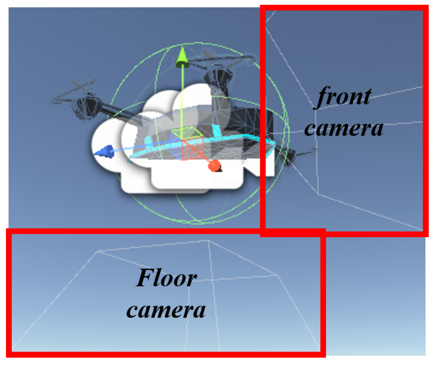
  • There is a floor camera of the drone to capture the floor QR codes.
  • The center of the floor camera is perpendicular to the floor.
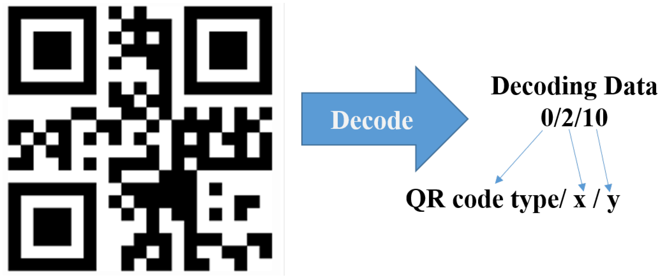
  • The absolute coordinate of the QR code is contained in the floor QR code.
  • The floor QR codes are attached in a fixed direction.
  • The size of the QR codes attached to the load are the same.
  • There is a camera on the front of the drone to capture the QR codes of the loaded objects.
  • During mapping, the central axis of the camera and the face of the loaded object where the QR code is located are perpendicular to each other.
  • The drone has basic knowledge of the size of the entire space.
Assumptions 1 and 6 can are depicted in Figure 4. The QR codes are attached to the floor where the drone flies and to the load.
Assumptions 2 and 7 are presented in Figure 5 and Figure 6, displaying the floor camera and the front camera of the drone for capturing the floor and load QR codes, respectively.
Assumptions 3 and 8 are depicted in Figure 7. They represent the perpendicularity between the optical axis of the camera and the surface of each QR code (floor and load).
Assumption 4 is illustrated in Figure 8. When decoding the QR code on the floor, the data “0/2/10” can be read, where 0 represents the QR code type. Zero represents the floor QR code, and 1 represents the load QR code. Additionally, 2 and 10 represent the x-coordinate and y-coordinate, respectively, of the QR code’s position in the absolute coordinate system.
Assumption 5 is depicted in Figure 9. The QR code must be attached in such a way that the finder pattern is fixed in a specific direction, as indicated in Figure 9. This paper assume that the finder pattern of the QR code is attached parallel to the y-axis of the absolute coordinate system.

3.2. Proposed Drone 3D Localization Algorithm

3.2.1. Overall Drone 3D Localization Algorithm

Algorithm 1 presents the overall process of the position estimation algorithm. The basic input for the position estimation algorithm is the image data (FloorFrame) captured through the floor-facing camera of Assumption 2. Once the FloorFrame is input, all QR codes in the image are detected and inserted into the QR_CODE_LIST (line 1). The variable MinDist is initialized as infinity to store the minimum distance between the image center and the QR code center (line 2). The image center point ( F C f x , F C f y ) of the FloorFrame is determined (line 3). The center point ( Q R f x , Q R f y ) of each QR code in the QR_CODE_LIST is determined, and the distance between this center point and the image center point ( F C f x , F C f y ) is calculated (lines 4–6), where Dist(P1, P2) is the formula to calculate the Euclidean distance between points P1 and P2. If the distance between the QR code center and image center is shorter than the existing MinDist, the information for the nearest QR code is updated (lines 7–9). The coordinates of the closest QR code center point ( M Q R f x , M Q R f y ) from the image center are also updated. The updated MinQR contains the position coordinates of the QR code in the world coordinate system ( Q R f x , Q R f y ), the length of one side of the QR code ( Q R L r ), and the distance information from the vertex of the QR code to the QR code center. Once the search for the closest QR code in the image to the image center is complete, the algorithm determines whether the minimum distance (MinDist) and distance between the two center points (( Q R f x , Q R f y ), ( F C f x , F C f y )) match using the threshold value Th. If MinDist is smaller than Th, the MatchedLocalization() algorithm is executed, assuming that the two center points match (lines 10–11). If MinDist is greater than Th, the NotMatchedLocalization() algorithm is executed, if the two center points do not match (lines 12–13).
Algorithm 1 Pseudocode of Drone 3D Localization  Algorithm
Input:
FloorFrame: Floor-direction camera image data
QR_CODE_LIST: All QR codes in the FloorFrame
( F C f x , F C f y ): Frame center point in image coordinates
( Q R f x , Q R f y ): QR code center point in image coordinates
MinDist: Minimum distance between the QR code center and frame center
( M Q R f x , M Q R f y ): position of the QR code closest to the frame center in the image
Th: Threshold to determine whether ( Q R f x , Q R f y ) and ( F C f x , F C f y ) match
MinQR: Information structure of the QR code closest to frame center
Structure of MinQR
[( Q R r x , Q R r y ): x and y coordinates of the QR code in world coordinates,
Q R L r : The length of one side of the QR code in world coordinates,
V C r : Distance from a vertex to the QR code center within the QR code]
Output:
( D r x , D r y , D r z ): x, y, and z positions of the drone in world coordinates
D r θ : Angle of the direction of the drone relative to the x-axis in world coordinates
Procedure Drone 3D Localization
1        QR_CODE_LISTInsert All QR Code Detection in FloorFrame
2        MinDist
3        ( F C f x , F C f y ) ← Center Point of FloorFrame
4        For QR To QR_CODE_LIST
5              ( Q R f x , Q R f y ) ← Center Point of QR
6              If MinDist > Dist( Q R f x , Q R f y ,( F C f x , F C f y )) Then
7                     MinDistDist(( Q R f x , Q R f y ),( F C f x , F C f y ))
8                     MinQR ← information from the QR
9                     ( M Q R f x , M Q R f y ) ← ( Q R f x , Q R f y )
10        If MinDist <= Th Then
11                ( D r x , D r y , D r z , D r θ )←MatchedLocalization(MinQR)
12        Else
13                ( D r x , D r y , D r z , D r θ )←NotMatchedLocalization(MinQR,( F C f x , F C f y ),( M Q R f x , M Q R f y ))
END
In Section 3.2.2 the method for detecting all QR codes in line 1 is explained. Section 3.2.3, details the method for detecting the QR code center points in line 5. Section 3.2.4 describes the meaning of the distance between the QR code center and image center in line 6. Then, Section 3.2.5 explains the MatchedLocalization() algorithm in line 11, and Section 3.2.6 clarifies the NotMatchedLocalization() algorithm in line 13.

3.2.2. QR Code Detection Using the QR Code Reader

When an image is input through the floor-facing camera, the QR codes in the image are detected using a QR code reader. The QR code reader uses Pyzbar [21] to detect QR codes, as illustrated in Figure 10. The red area indicates where the QR code is located, and the blue area indicates the segmented area of the detected QR code.

3.2.3. Detecting QR Code Center Points

After the QR code is detected on the image, the center points of all QR codes are detected. The reason for detecting the center point of a QR code is that, even with various rotational movements, the center axis of the QR code remains constant, as illustrated in Figure 11c–f. However, due to Assumption 3, situations like those shown in Figure 11d–f do not occur in this study.
As depicted in Figure 10 in Section 3.2.2, the areas containing the QR code (red rectangle) and the QR code segmentation (blue rectangle) are represented as shown in Figure 12a. The two rectangles have the same center point, so the intersection point of the diagonals of the red rectangle is set as the center point of the QR code, as indicated in Figure 12b.

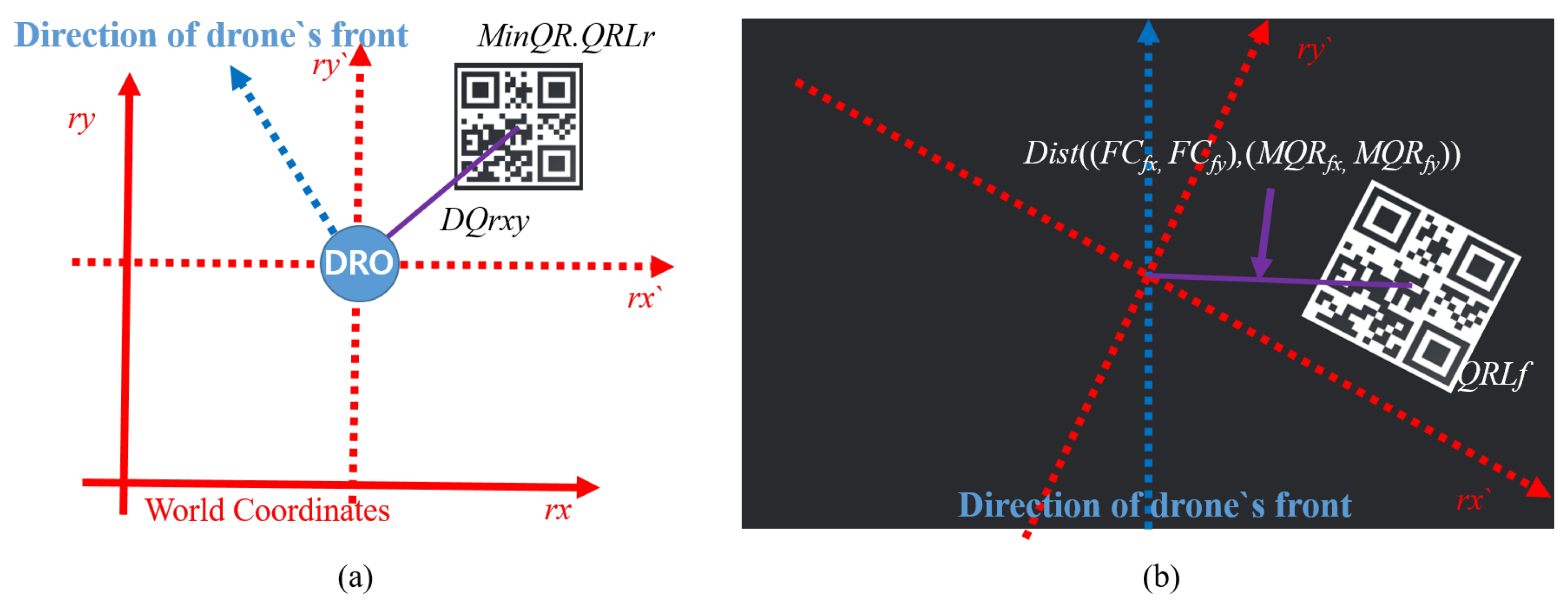
3.2.4. Distance between Image Center and QR Code Center

The distance between the image center and the QR code center is illustrated in Figure 13, where the purple point represents the image center (( F C f x , F C f y )), the green point represents the center of the closest QR code to the image center (( M Q R f x , M Q R f y )), and the blue rectangle represents the closest QR code (MinQR). In this case, if the distance between the green and purple points is the shortest MinDist, and this distance falls within the radius of the blue circle (Th) in the figure, the centers match.

3.2.5. Localization Method of a Drone When the QR Center and Image Center Match

Algorithm 2 presents the localization algorithm in the case where the QR center and image center match(MatchedLocalization). The input is MinQR, which is received from the Localization(). In addition, MinQR contains the position coordinates of the QR code in the world coordinate system ( Q R r x , Q R r y ), the length of one side of the QR code ( Q R L r ), and the distance from the vertex of the QR code to its center. In addition, information about the length of one side of the QR code in the image coordinate system ( Q R L f ) is required. The algorithm outputs the drone position coordinates ( D r x , D r y , D r z ) and angle ( D r θ ) with respect to the x-axis in the actual coordinate system. Further, FL represents the focal length of the camera.
Algorithm 2 Pseudocode of MatchedLocalization  Algorithm
Input:
MinQR: Information structure of the QR code closest to the frame center
Structure of MinQR
[( Q R r x , Q R r y ): x and y coordinates of the QR code in world coordinates,
Q R L r : The length of one side of the QR code in world coordinates,
V C r : Distance from a vertex to the QR code center within the QR code]
Q R L f : The length of one side of QR code in image coordinates
Output:
( D r x , D r y , D r z ): x, y, and z positions of drone in world coordinates
D r θ : Angle of the direction of the drone relative to the x-axis in world coordinates
Procedure MatchedLocalization
1         D r θ ← Extracting angles based on the MinQR shape
2         Q R L f ← Average of all side lengths of MinQR
3         D r z M i n Q R . Q R L r × FL/ Q R L f
4         D r y M i n Q R . Q R r x
5         D r y M i n Q R . Q R r y
END
The algorithm first determines D r θ (line 1). The meaning of D r θ can be understood through Figure 14a, where D r θ represents the angle between the x-axis of the world coordinate system and the direction in which the drone is facing.
The method of estimating the angle the drone is facing using QR codes is related to Assumption 5, where QR codes are attached in a fixed orientation, so the floor QR code rotates in the same direction as the drone. This method is explained in Figure 14b, where the red lines represent the directions of the x- and y-axes in the actual absolute coordinate system. The blue line represents the direction the drone is facing. Therefore, using the degree of rotation of the QR code allows us to determining the degree of rotation of the drone.
The rotated angle of the QR code can be determined, as illustrated in Figure 15. First, when an image containing the QR code is provided, as displaying in Figure 15a, the finder patterns are located. Then, as depicted in Figure 15b, the centroid of the finder patterns is located. Next, the centroid points of the finder patterns are used, as depicted in Figure 15c, to calculate the direction in which the drone is facing, as shown in Figure 15d. The orientation of the QR code is fixed (according to Assumption 5), and the forward direction of the drone corresponds to the 12 o’clock direction in the input image (indicated by the blue arrow). Therefore, the rotated angle D r θ can be computed.
The method for estimating the drone position ( D r x , D r y , D r z ) is described in lines 2–5 in table. The camera pinhole model is used to estimated the altitude of the drone. When applying this to the actual QR code-based approach, it can be modeled as illustrated in Figure 16. In the figure, MinQR Q R L r represents the actual length of a QR code side and Q R L f denotes the length of the QR code side in the image. In addition, FL denotes the focal length. Equation (1) can be derived according to the geometric properties of the camera pinhole model and by rearranging it, Equation (2) can be obtained. This approach allows us to determine D r z (line 3 in the table), and update D r x and D r y with the QR code’s position coordinates (lines 4–5 in the table).
D r z : F L = M i n Q R . Q R L r : Q R L f
D r z = M i n Q R . Q R L r × F L / Q R L f

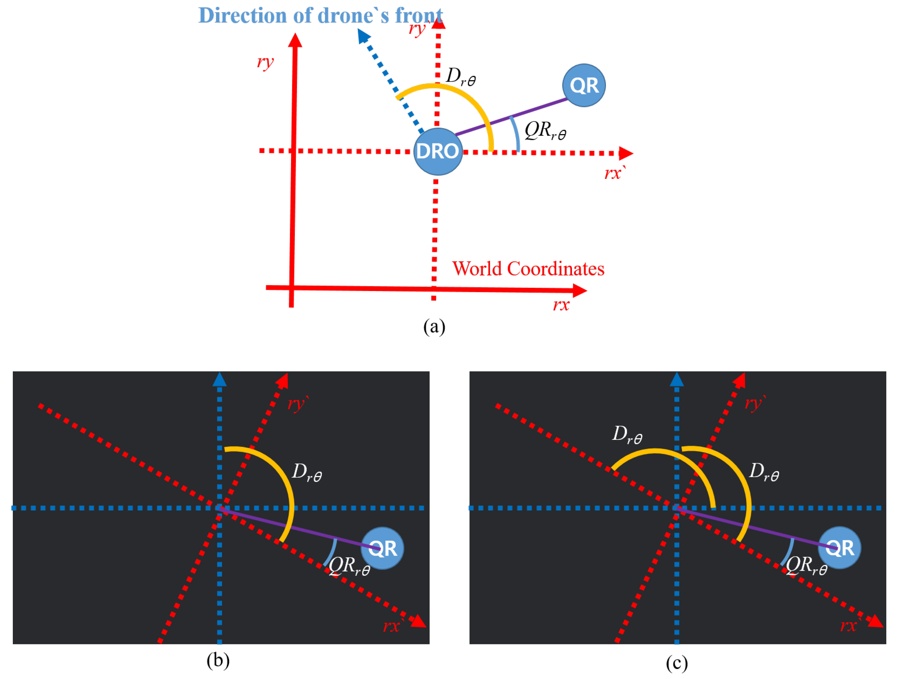
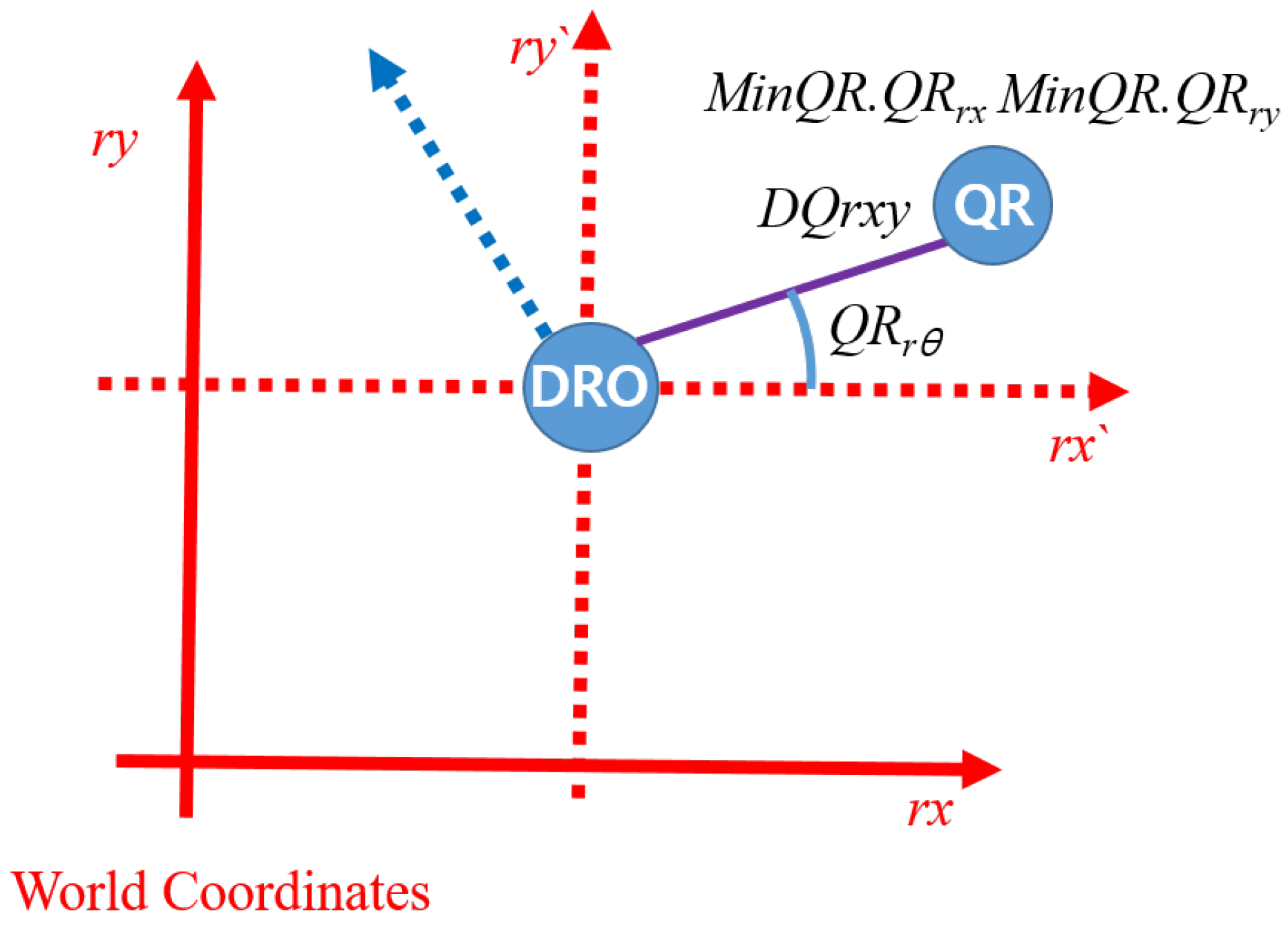
3.2.6. Drone Localization Method When the QR Center and Image Center Not-Matched

Algorithm 3 presents the algorithm for estimating the position when the QR code centers do not match. The algorithm takes several inputs: the QR code closest to the image center (MinQR), coordinates of the image center in the image coordinate system ( F C f x , F C f y ), coordinates of the QR code closest to the image center in the image coordinate system ( M Q R f x , M Q R f y ), the length of the QR code side in the image ( Q R L f ), the distance from the QR code center to its corner in the image coordinate system ( V C f ), the distance between the QR code and the drone projected onto the xy-plane in the world coordinate system ( D Q r x y ), and the angle between the line segment DQrxy and the x-axis in the world coordinate system ( Q R r θ ). The outputs of the algorithm are the drone’s position coordinates ( D r x , D r y , D r z ) in the world coordinate system and the angle ( D r θ ) with respect to the x-axis.
The algorithm begins by calculating the length of the QR code diagonal in the image ( V C f : line 1) and computes the average length from the image center to the QR code center and each corner, as illustrated in Figure 17. Then, following the method mentioned in Section 3.2.6, the algorithm determines D r θ (line 2).
Algorithm 3 Pseudocode for NotMatchedLocalization  Algorithm
Input:
MinQR: Information structure of the QR code closest to the frame center
Structure of MinQR
[( Q R r x , Q R r y ): x and y coordinates of the QR code in world coordinates,
Q R L r : The length of one side of the QR code in world coordinates,
V C r : Distance from a vertex to the QR code center within the QR code]
( F C f x , F C f y ): Frame center point in image coordinates
( M Q R f x , M Q R f y ): Position of the QR code closest to the frame center in image coordinates
Q R L f : Length of one side of the QR code in image coordinates
V C f : Distance between the vertex to QR code center in image coordinates
D Q r x y : Distance between the drone and QR code projected on the xy plane in world coordinates
Q R r θ : Angle formed by x-axis and the line D Q r x y in world coordinates
Output:
( D r x , D r y , D r z ): x, y, and z positions of the drone in world coordinates
D r θ : Angle of the direction of the drone relative to the x-axis in world coordinates
Procedure NotMatchedLocalization
1         V C f ← Average of the distance sum between ( M Q R f x , M Q R f y ) and each vertex of MinQR
2         D r θ ← Extracting angles based on the MinQR shape
3         D r z MinQR. V C r × FL/ V C f
4         D Q r x y M i n Q R . Q R L r × Dist(( F C f x , F C f y ),( M Q R f x , M Q R f y ))/ Q R L f
5         Q R r θ ← Angle between two lines,
                         y ← tan( D r θ ) × (x − F C f x ) + F C f y   a n d y = ( Q R f x F C f x )/( Q R f y F C f y ) × (x − F C f x ) + F C f y
6         D r x M i n Q R . Q R r x D Q r x y × cos( Q R r θ )
7         D r y M i n Q R . Q R r x D Q r x y × sin( Q R r θ )
END
The next step is to calculate the drone height ( D r z ) (line 3). The modeling method in Figure 18 is used to determine D r z . Symmetry is achieved by modeling a triangle with vertices (world vertex, cl, ( M i n Q R . Q R r x , M i n Q R . Q R r y )) and another triangle with vertices (frame vertex, cl, ( M Q R f x , M Q R f y )) leading to the derivation of Equation (3). Additionally, symmetry is achieved by considering the triangle(( F C f x , F C f y ), cl, ( MinQR.Q R r x , MinQR.Q R r y )) and another triangle(O, cl, ( MinQR.Q R r x , MinQR.Q R r y )) allowing the formulation of Equation (4). Therefore, Equation (5) can be derived by rearranging Equations (3) and (4):
( ( M Q R f x , M Q R f y ) , c l ) : ( ( M i n Q R . Q R r x , M i n Q R . Q R r y ) , c l ) = V C f : M i n Q R . V C r
( ( M Q R f x , M Q R f y ) , c l ) : ( ( M i n Q R . Q R r x , M i n Q R . Q R r y ) , c l ) = F L : D r z
D r z = i n Q R . V C r × F L / V C f
The next step involves calculating the x- and y-coordinates ( D r x , D r y ) of the drone in the world coordinate system (lines 4–7). To do this, we must determine D Q r x y and Q R r θ as indicated in Figure 19, where D Q r x y represents the distance between the drone and QR code center projected onto the xy plane in the world coordinate system, and Q R r θ represents the angle between D Q r x y and the x-axis in the world coordinate system.
The variable D Q r x y can be modeled as presented in Figure 20 (line 4), where D Q r x y corresponds to Dist(( F C f x , F C f y ), ( M Q R f x , M Q R f y )) and M i n Q R . Q R L r corresponds to Q R L f , resulting in the derivation of Equation (6). Simplifying Equation (6) leads to Equation (7).
D Q r x y : M i n Q R . Q R L r = D i s t ( ( F C f x , F C f y ) , ( M Q R f x , M Q R f y ) ) : Q R L f
D Q r x y = M i n Q R . Q R L r × D i s t ( ( F C f x , F C f y ) , ( M Q R f x , M Q R f y ) ) / Q R L f
The next step is to calculate Q R r θ (line 5). The method for calculating Q R r θ can be explained using Figure 21. In Figure 21a, D r θ , is already computed. Figure 21b illustrates the relationship between D r θ , the drone, the QR code, and the xy plane in the image. Moreover, D r θ represents the angle between the x-axis and the direction the drone faces in reality and is equivalent to the angle formed between the line crossing the image center point and rx’ as depicted in Figure 21c. Therefore, we can obtain the equations for the straight lines: the line of the segment D Q r x y (purple line) with the image center point ( F C f x , F C f y ) as the origin and the line of rx’ (Equations (8) and (9)). Q R r θ is calculated using these equations:
y = t a n ( D r θ ) × ( x F C f x ) + F C f y
y = ( Q R f x F C f x ) / ( Q R f y F C f y ) × ( x F C f x ) + F C f y
Finally, we compute D r x and D r y (line 6–7). This step, we can establishes a relationship between the actual QR code and drone, as depicted in Figure 22. Based on this relationship, we can derive Equations (10) and (11):
D r x = M i n Q R . Q R r x D Q r x y × c o s ( Q R r θ )
D r y = M i n Q R . Q R r y D Q r x y × s i n ( Q R r θ )

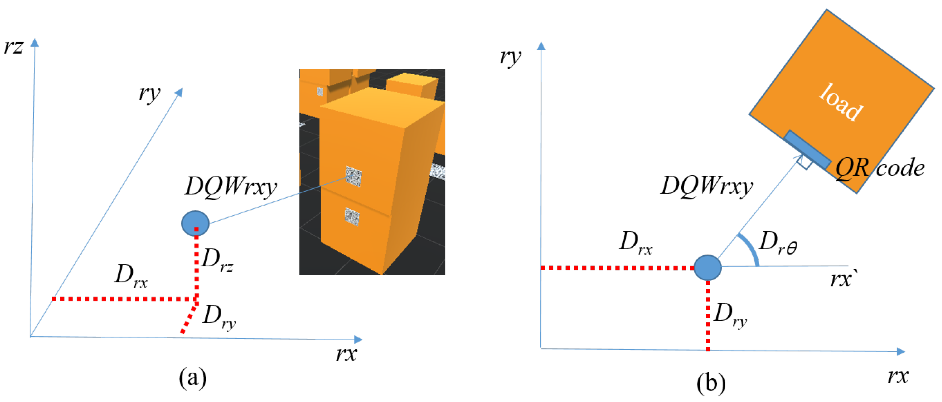
3.3. Proposed Load Mapping Algorithm

3.3.1. Load Mapping Algorithm Overview

Algorithm 4 presents the entire process of the mapping algorithm, which takes the following inputs: the image from the front-facing camera (LoadFrame), coordinates of the image center ( F C f x , F C f y ), the coordinates of the QR code center in the image ( Q R f x , Q R f y ), the threshold value (Th) to determine if the image center and QR code center match, the drone’s position coordinates ( D r x , D r y , D r z ) obtained through the localization algorithm, and viewing direction angle of the drone with respect to the x-axis in the world coordinate system. The algorithm outputs the position coordinates of all detected QR codes in the LoadFrame.
Algorithm 4 Pseudocode of LoadMapping  Algorithm
Input:
LoadFrame: Face-direction camera image data
( F C f x , F C f y ): Frame center point in image coordinates
( Q R f x , Q R f y ): QR code center point in image coordinates
Th: Threshold to determine whether ( Q R f x , Q R f y ) and ( F C f x , F C f y ) match
( D r x , D r y , D r z ): x, y, and z positions of drone in world coordinates
D r θ : Angle of the direction the drone relative the x-axis in world coordinates
Output:
( Q R r x , Q R r y , Q R r z ): x, y, and z position of the QR code in world coordinates
LOAD_QR_POSITION: Location of all QR codes in image coordinates
Procedure LoadMapping
1        QR_CODE_LISTInsert All QR Code Detection in LoadFrame
2        ( F C f x , F C f y ) ← Center Point of LoadFrame
3        For QR To QR_CODE_LIST
4                ( Q R f x , Q R f y ) ← Center point of QR
5                If Dist(( Q R f x , Q R f y ),( F C f x , F C f y )) <= Th Then
6                        ( Q R r x , Q R r y , Q R r z ) ← MatchedMapping(QR, D r x , D r y , D r z , D r θ )
7                Else
8                        ( Q R r x , Q R r y , Q R r z ) ←NotMatchedMapping(QR, D r x , D r y , D r z , D r θ ,
                                                                        ( F C f x , F C f y ),( Q R f x , Q R f y ))
9                LOAD_QR_POSITIONInsert ( Q R r x , Q R r y , Q R r z )
END
The LoadMapping algorithm detects all QR codes using a QR code reader (line 1) and determines the image center (line 2). For each QR code, it calculates the center point (line 4) and compares the Euclidean distance between the QR code’s center point and the image center with a threshold value (Th) to determine if they match (line 5). If the distance is less than or equal to the threshold, it generates a load map for the matched case (line 6). Otherwise, the algorithm generates a load map for the unmatched case (lines 7–8). The algorithm identifies and stores the positions of the QR codes by performing these steps for all QR codes in the image (line 9). Section 3.3.2 describes the load map generation algorithm (MatchedMapping()) for matched QR codes where the center point matches the image center, while Section 3.3.3 explains the load map generation algorithm (NotMatchedMapping()) for situations where the center point does not match the image center.

3.3.2. Load QR Code Mapping Algorithm When Center Points Matched

Algorithm 5 describes the MatchedMapping() algorithm operation. It requires the following input values: basic information about the load QR code (QR), estimated drone position information ( D r x , D r y , D r z ), drone viewing angle ( D r θ ), QR code side length in the image coordinate system ( Q R L f ), and distance between the QR code and drone in the world coordinate system ( D Q W r x y ). However, this algorithm focuses on determining the position of the load QR code and generating a map; thus, the QR code information does not include its coordinates in the world coordinate system.
Algorithm 5 Pseudocode of MatchedMapping  Algorithm
Input:
QR: Information structure of the load QR code
Structure
[ Q R L r : The length of one side of the QR code in world coordinates,
V C r : Distance from a vertex to the QR code center within the QR code]
( D r x , D r y , D r z ): x, y, and z positions of the drone in world coordinates
D r θ : Angle of the direction of the drone relative to the x-axis in world coordinates
Q R L f : The length of one side of the QR code in image coordinates
D Q W r x y : Distance between the drone and wall attaching the load QR code in world coordinates
Output:
( Q R r x , Q R r y , Q R r z ): x, y, and z positions of QR code in world coordinates
Procedure MatchedMapping
1         D Q r x y FL × Q R . Q R L r / Q R L f
2         Q R r x D r x + D Q r x y × cos( D r θ )
3         Q R r y D r y + D Q r x y × sin( D r θ )
4         Q R r z D r z
END
The situation assumed in MatchedMapping starts from Assumption 8, referring to a scenario where the frontal camera center aligns with the load QR code center of the drone, as depicted in Figure 23a. In this case, the height ( Q R r z ) of the load QR code in the world coordinates matches the current height of the drone ( D r z ). Additionally, Q R r x and Q R r y are modeled as illustrated in Figure 23b, representing the situation viewed in the xy-plane where the centers align. The blue dot represents the drone’s position, “load” represents the load, and the blue rectangle inside the load represents the load QR code. Given the current drone position ( D r x , D r y , D r z ) and the drone’s frontal angle of view ( D r θ ) obtained from the localization algorithm, we can derive the equations as shown in lines 2–4.
The variable D Q W r x y represents the distance from the actual QR code to the drone. To calculate this distance, we can model it similarly to the situation where the center points are aligned in the localization algorithm, as depicted in Figure 24 (line 1).

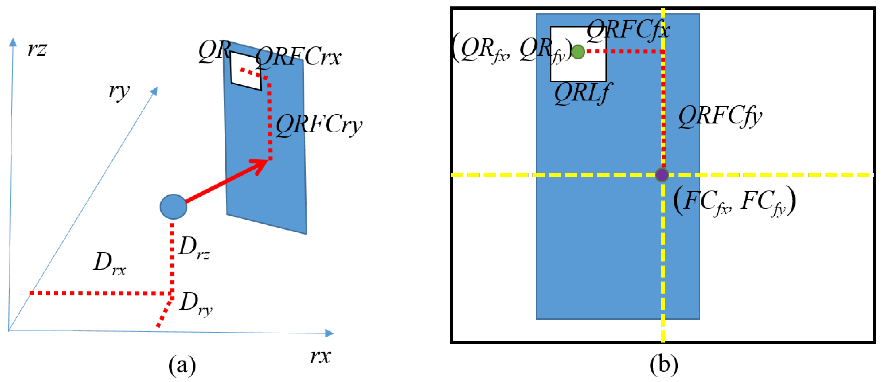
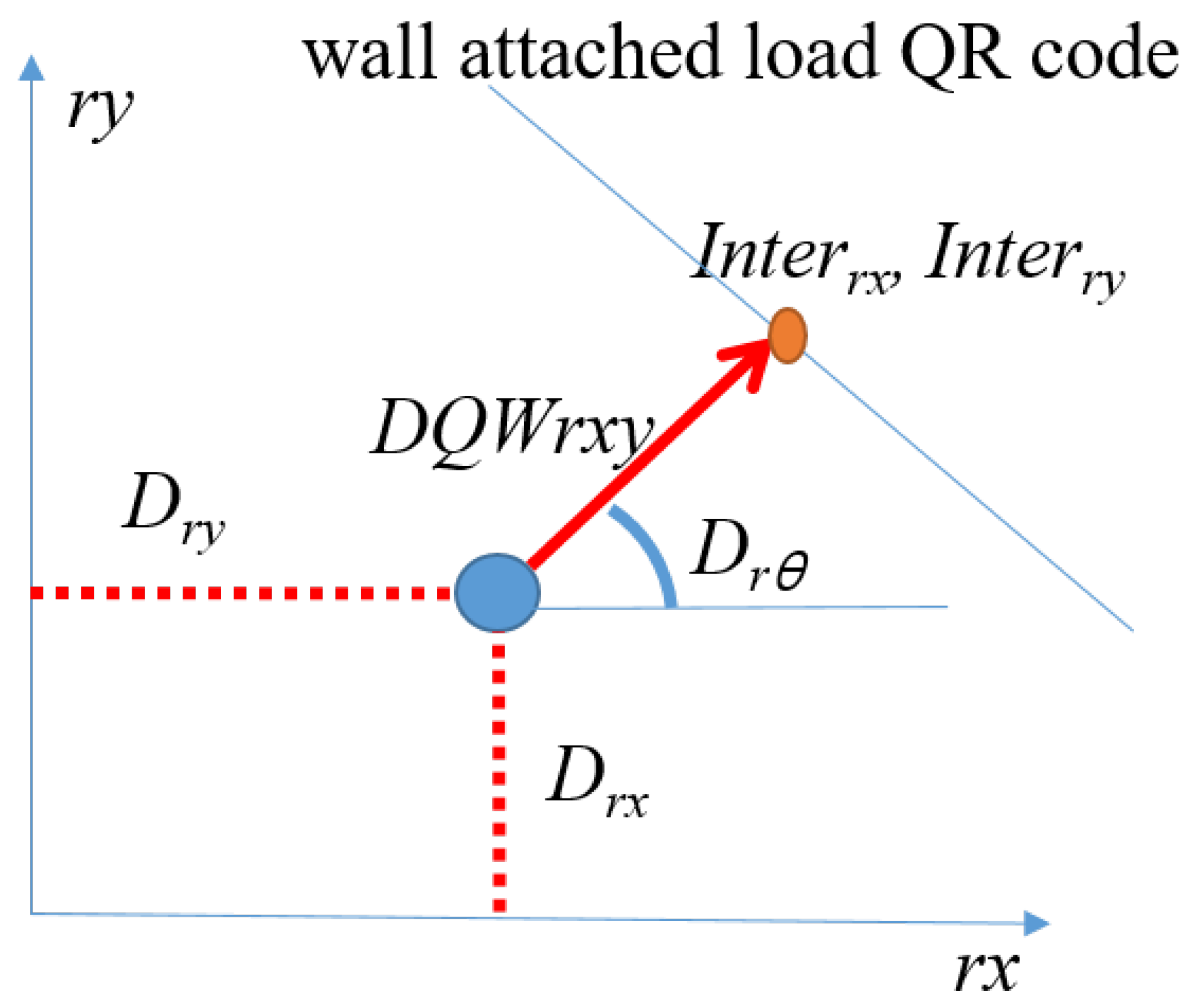
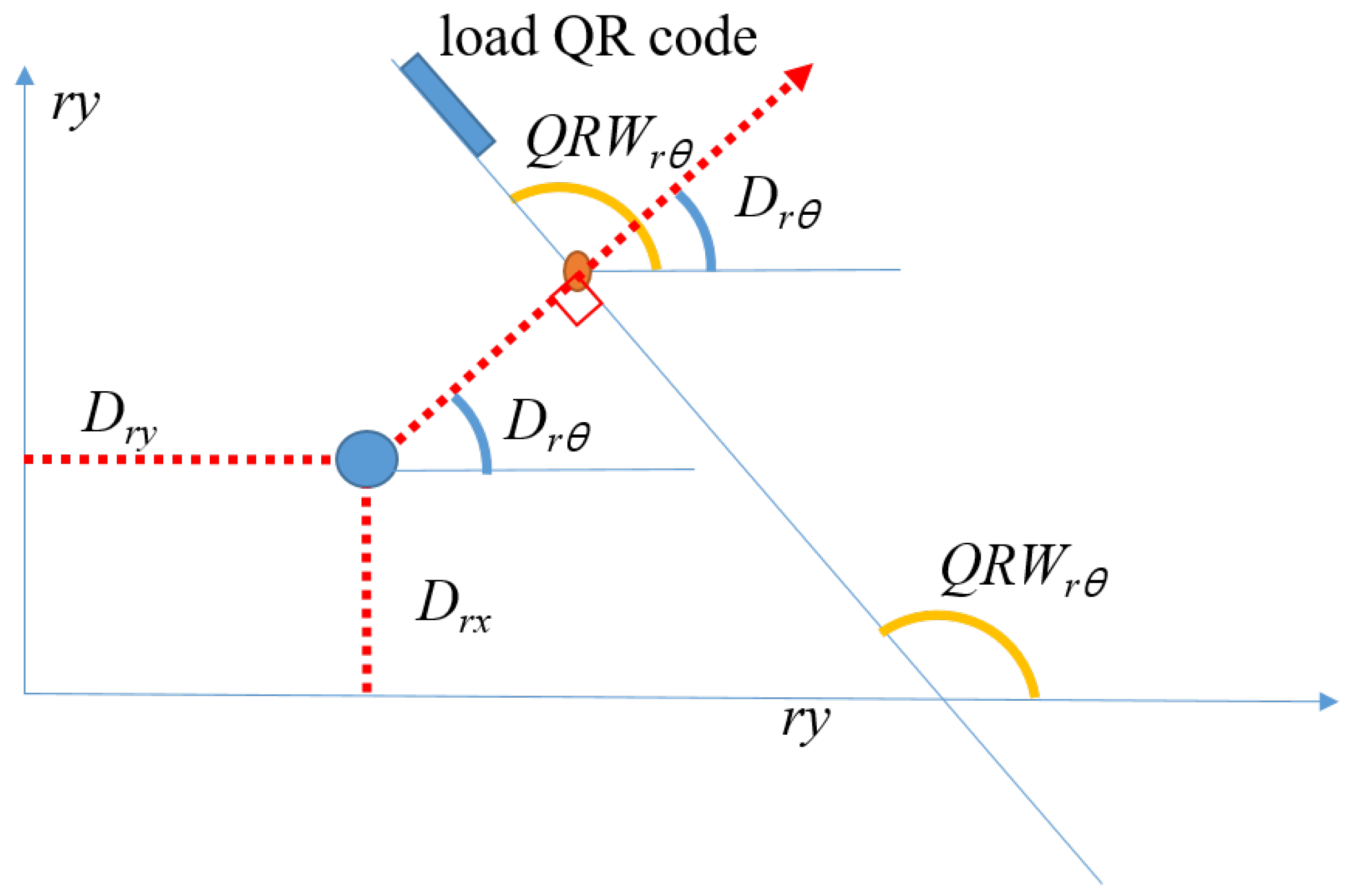
3.3.3. Load QR Code Mapping Algorithm with Center Point Not-Matched

Algorithm 6 describes the NotMatchedMapping algorithm operation. The algorithm requires the following input values: basic information on the load QR code (QR), image coordinates of the image center ( F C f x , F C f y ) and QR code center ( Q R f x , Q R f y ), estimated drone-position information ( D r x , D r y , D r z ), angle the drone is facing ( D r θ ), length of the QR code side in the image coordinate system ( Q R L f ), distances from the image center to the QR code center along the x-axis and y-axis ( Q R F C f x , QR F C f y ), corresponding distances in the world coordinate system ( Q R F C r x , Q R F C r y ), distance from the drone to the wall where the QR code is attached in the world coordinate system ( D Q W r x y ), coordinates of the intersection point between segment D Q W r x y and the wall where the QR code is attached ( I n t e r r x , I n t e r r y ), and the angle between the x-axis and the wall where the QR code is attached in the world coordinate system ( Q R W r θ ).
Algorithm 6 Pseudocode of NotMatchedMapping  Algorithm
Input:
QR: Information structure of load QR code
Structure
[ Q R L r : The length of one side of the QR code in world coordinates,
V C r : Distance from a vertex to the QR code center within the QR code]
( F C f x , F C f y ): Frame center point in image coordinates
( Q R f x , Q R f y ): QR code center point in image coordinates
( D r x , D r y , D r z ): x, y, and z positions of the drone in world coordinates
D r θ : Angle of the direction of the drone relative to the x-axis in world coordinates
Q R L f : The length of one side of the QR code in image coordinates
( Q R F C f x , QR F C f y ): The x and y-axes distance from the QR code
center to the frame center in image coordinates
( Q R F C r x , Q R F C r y ): Distance corresponding to ( Q R F C f x , QR F C f y )
in world coordinates
D Q W r x y : Distance between the drone and the wall attaching the load QR code in world coordinates
( I n t e r r x , I n t e r r y ): Position where the wall attaching the load QR code and the line
D Q W r x y intersect in world coordinates
Q R W r θ : Angle between the wall attaching the QR code and the x-axis in world coordinates
Output:
( Q R r x , Q R r y , Q R r z ): x, y, and z positions of the QR code in world coordinates
Procedure NotMatchedMapping
1        ( Q R F C f x , QR F C f y ) ←(| F C f x Q R f x |, | F C f y Q R f y |)
2        ( Q R F C r x , Q R F C r y ) ← ( Q R F C f x , QR F C f y ) × Q R . Q R L r / Q R L f
3         V C f ← Average of the distance sum between ( M Q R f x , M Q R f y ) and each vertex of QR
4         D Q W r x y QR. V C r × FL/ V C f
5        ( I n t e r r x , I n t e r r y ) ←( D r x + D Q W r x y × cos( D r θ ), D r y + D Q W r x y × sin( D r θ ))
6         Q R W r θ ←( D r θ + 90)% 360
7        If  F C f y > Q R f y
8                  Q R r z D r z + Q R F C r y
9        Else
10                 Q R r z D r z Q R F C r y
11         If  D r θ = 0
12                 Q R r x D r x + D Q W r x y
13                If  Q R f x > F C f x
14                         Q R r y D r y + Q R F C r x
15                Else
16                         Q R r y D r y Q R F C r x
17         Else If  D r θ = 90
18                 Q R r y = D r y + D Q W r x y
19                If  Q R f x > F C f x
20                         Q R r x D r x Q R F C r x
21                Else
22                         Q R r x D r x + Q R F C r x
23         Else If  D r θ = 180
24                 Q R r x D r x D Q W r x y
25                If  Q R f x > F C f x
26                         Q R r y D r y Q R F C r x
27                Else
28                         Q R r y D r y + Q R F C r x
29         Else If  D r θ = 270
30                 Q R r y D r y D Q W r x y
31                If  Q R f x > F C f x
32                         Q R r x D r x Q R F C r x
33                Else
34                         Q R r x D r x + Q R F C r x
35         Else
36                If  Q R f x > F C f x
37                         Q R r x I n t e r r x + Q R F C r x × cos( Q R W r θ )
38                         Q R r y I n t e r r y + Q R F C r x × sin( Q R W r θ )
39                Else If  Q R f x = F C f x
40                         Q R r x I n t e r r x
41                         Q R r y I n t e r r y
42                Else
43                         Q R r x I n t e r r x  + Q R F C r x × cos(( Q R W r θ + 180)%360)
44                         Q R r y I n t e r r y  + Q R F C r x × sin(( Q R W r θ + 180)%360)
END
The NotMatchedMapping algorithm operates in a situation where the image center of the front (load) camera does not align with the center of the load QR code, as illustrated in Figure 25a. When observing this situation through the front (load) camera, the resulting image is depicted in Figure 25b. With this information, Q R F C f x and QR F C f y can be obtained in line 1 and Q R F C r x and Q R F C r y can be derived in line 2. To calculate D Q W r x y , we can use the modeling in Figure 26, which is the same as that the localization algorithm for the mismatch situation. With this, D Q W r x y can be calculated in line 4. Next, we determine the height of the QR code ( Q R r z ), which can be derived from Figure 25b (lines 7–10). If the QR code center is above the image center in the image coordinate system (line 7), then Q R r z in the world coordinate system is equal to D r z + Q R F C r y (line 8). If the opposite situation occurs (line 9), Q R r z becomes D r z Q R F C r y (line 10).
To obtain Q R r x and Q R r y , we need to determine ( I n t e r r x , I n t e r r y ) as indicated in Figure 27. In addition, ( I n t e r r x , I n t e r r y ) refers to the x and y coordinates where the line passing through the center of the front camera and the wall where the QR code is attached intersects. We can derive this in line 5 of the algorithm.
To determine the angle Q R W r θ formed by the wall where the QR code is attached and the x-axis in the absolute coordinate system, we refer to Figure 28. In NotMatchedMapping algorithm, line 6 can be derived based on this information. The reason the direction the drone is facing and the wall where the QR code is attached are perpendicular is Assumption 8.
The next step involves the modeling process to determine Q R r x and Q R r y , which varies slightly depending on the magnitude of D r θ , as illustrated in Figure 29. When D r θ is 90 (Figure 29b), we can determine Q R r x and Q R r y based on the position of the QR code in the image captured by the drone’s front camera. This can be performed using lines 17–22 of the algorithm. In the case where D r θ is 180 (Figure 29c), we can determine Q R r x and Q R r y based on the position of the QR code in the image captured by the front camera of the drone using lines 23–28 of the algorithm. When D r θ is 270 (Figure 29d), we can determine Q R r x and Q R r y based on the position of the QR code in the image captured by the front camera of the drone. This can be done using lines 29–34 of the algorithm. For any other value of D r θ , (Figure 29e), we can determine QR r x and Q R r y based on the position of the QR code in the image captured by the front camera using lines 35–44 of the algorithm.

4. Experimental Results

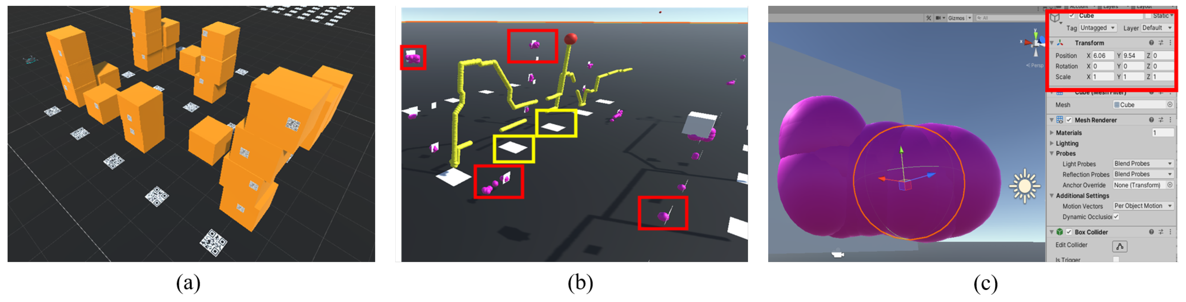
4.1. Experiment on Simulator

4.1.1. Experimental Environment on Simulator

Simulator experiments and actual drone experiments were conducted to evaluate the performance of the proposed algorithm based on the given assumptions. The simulator, depicted in Figure 30a, allows for a flexible setup of the experimental environment. Cameras were attached underneath and in the front of the drone, Figure 30b, enabling the simultaneous recording of two videos to easily synchronize between them. Additionally, the simulator incorporated the positional information of the drone automatically, as illustrated in Figure 30c, enabling real-time logging of data for comparison.

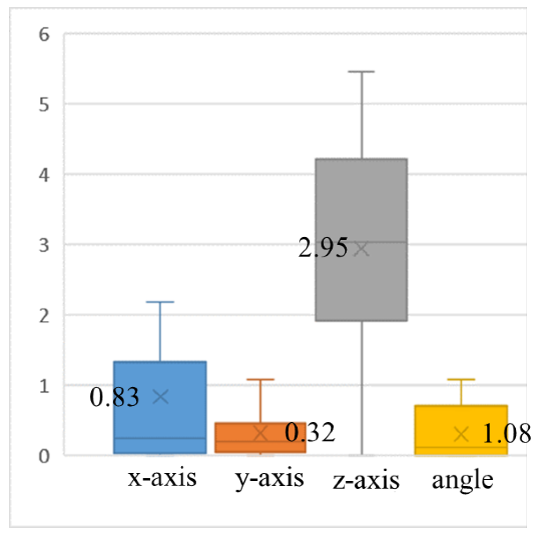
4.1.2. Experimental Results for Drone’s 3D Localization

Table 1 presents example data for the experimental results. The performance measure of the experiment compares the actual drone position (a) obtained from the simulator with the estimated drone position (b) derived from the images, specifically in terms of the differences in the x-, y-, and z-coordinates (|(a) − (b)|). In addition, D r θ represents the forward direction of the current drone. Full experimental results can be found in Table A1Table A4.
We collected 50 data points similar to those in Table 1. Figure 31 is a box plot graph summarizing the results of the entire dataset. According to the experimental results, the average errors along the x, y, and z axes were approximately 0.83, 0.32, and 2.95 cm, respectively. The angular error was approximately 1.08 degrees.
Figure 32 visually represents the logged data of the actual path taken by the drone in the simulator and the estimated path obtained by the proposed positioning estimation algorithm. The red line in the figure represents the actual path taken by the drone in the simulator, whereas the yellow line represents the estimated path generated by the proposed positioning estimation algorithm. In Figure 32a, viewed from a vertical perspective, the x- and y-axes closely align, appearing overlapped. However, in Figure 32b, viewed from a side angle a consistent error occurs along the z-axis.

4.1.3. Experimental Results for LoadMapping Algorithm

Simulator experiments were conducted to measure the accuracy of the mapping algorithm. The simulator in Figure 33 was created where an environment was set up with floor QR codes and attached payload QR codes (Figure 33a). The drone was then maneuvered in the simulator while simultaneously capturing images of the floor and payload. The mapping results for the payload QR code positions were visualized, as shown in Figure 33b. In the figure, the purple spheres represent the visualized positions of the QR codes estimated by the mapping algorithm. The white rectangles (dark-colored rectangles) attached to the floor in Figure 33b represent the floor QR codes that are not estimated. The positions of the payload QR codes (red rectangles) are represented by the center coordinates of the purple spheres. The center coordinates of the purple spheres are observed in Figure 33c. Subsequently, the averages were compared by randomly selecting five purple spheres (estimated results) from QR codes with five or more purple spheres.
Table 2 presents the some results of the mapping algorithm measured using the simulator. For the QR codes in the simulator, the average errors were approximately 0.87 cm along the x-axis, 1.64 cm along the y-axis, and 2.11 cm along the z-axis. This result can also be confirmed through Figure 34. These results are consistent with the observations in Figure 33c, where the estimated positions (purple spheres) are densely clustered around the actual QR code positions (white rectangles). Full experimental results can be found in Table A5.

4.2. Experiment Using Actual Drone

4.2.1. Experimental Environment Using Actual Drone

The experimental setup using an actual drone was configured as depicted in Figure 35. As shown in Figure 35a, an origin point and coordinate plane were established on the floor, with markings (black lines) made every 1 m on the floor. Floor QR codes were then attached at the intersections of these markings. In Figure 35b, the drone was flown to capture images of the floor QR codes. The proposed algorithm was applied to the captured footage to extract predicted results, which were compared to the actual position of the drone. For the actual position of the drone, as shown in Figure 35b, a sinker was attached to the drone. The actual x and y coordinates of the drone were measured relative to the position of the sinker on the floor, while the z-axis was measured based on the length of the line connected to the sinker. The drone used in the experiment was the DJI Mavic Mini 3 Pro(manufacturer: DJI, country: China).

4.2.2. The Experimental Results of Localization Algorithm Using an Actual Drone

Table 3 presents the experimental results of localization accuracy based on actual drone experiments. In this experiment, due to the inability to accurately measure angles, only information along the x, y, and z axes was utilized to assess accuracy.
The experimental results show an average error of 1.55 cm, 0.51 cm, and 2.04 cm along the x, y, and z axes, respectively. Comparing these results with simulator experiments, the average errors along the x and y axes increased by approximately 0.57 cm and 0.41 cm, respectively. However, the overall error remained relatively consistent.

4.2.3. The Experimental Results of Load Mapping Algorithm Using an Actual Drone

In the load mapping experiment using an actual drone, an environment was set up by adding cargo QR codes, as shown in Figure 36. Building upon the setup described in Figure 35a, load QR codes were added to the wall to create the experimental environment.
The experimental results of the load mapping algorithm using an actual drone are presented in Table 4. The average errors observed were approximately 2.19 cm along the x-axis, 2.70 cm along the y-axis, and 6.36 cm along the z-axis. It is evident that these errors are larger than those presented in the simulator. Several reasons can account for these results. Firstly, errors may arise due to lens distortion. Secondly, changes in the drone’s position during hovering may contribute to inaccuracies. Lastly, difficulties in achieving perfect vertical alignment between the front camera and the wall surface could also contribute to the observed discrepancies.

4.3. Commercial Drone GPS-Based Average Error Experiment

In this section, we aim to measure the errors generated by the GPS-based positioning system mounted on the actual drone used in the experiment. To conduct the experiment, we set up the experimental environment as depicted in Figure 37a. QR codes were placed on the floor at 1 m intervals, with a red circle serving as the reference point. The drone was then positioned on top of these QR codes, and latitude and longitude were measured using the drone’s GPS. Additionally, as shown in Figure 37b, we assigned numbers to the QR codes and used QR1 as the reference point to establish the distances to each QR code (QR2 9) for comparison, serving as the ground truth for evaluation.
Before explaining the experimental results, it is necessary to determine the distance equivalent to one degree of latitude and longitude around the experimental location. Within the latitude range of 35 to 40 degrees, the distance per degree of latitude is approximately 110.941 to 111.034 km, while the distance per degree of longitude ranges from about 91.290 to 85.397 km. Since South Korea spans approximately latitude 37 degrees, we can calculate that one degree of latitude corresponds to approximately 110.988 km (11,098,800 cm) and one degree of longitude corresponds to approximately 88.343 km (8,834,300 cm). These values will be used to convert latitude and longitude differences into centimeters in Table 5.
The experimental results can be observed through Table 5. In summarizing the experimental results, latitude and longitude values were recorded up to the sixth decimal point to ensure maximum precision. Using the drone, latitude and longitude values were measured for QR2 through QR9, and the differences from QR1 were calculated. These differences were then converted into centimeters and used in distance measurement formulas to calculate the distances from QR1.
The results indicated that QR7 exhibited the least error at 9.130598 cm, while QR6 showed the largest error at 113.058256 cm. On average, an error of 67.361937 cm was observed. Comparing these results to the method presented in this paper, which showed errors ranging from 0 to 3 cm, it is evident that the proposed method outperforms the GPS mounted on the actual drone. Additionally, while GPS-based errors have a wide range, the proposed method offers a much narrower error range, highlighting its advantages.

5. Conclusions

The utilization of drones has diversified as the Fourth Industrial Revolution has continued to expand. Among various applications, this paper focuses on load management using drones. In general, when using autonomous drones, GPS receivers attached to the drones are used to determine the drone position. However, GPSs integrated into commercially available drones have an error margin on the order of several meters. To compensate for this, high-precision GPSs or drones equipped with such systems could be used, but they are expensive.
Additionally, in the context of load management applying drones, recent research has explored methods utilizing RFID and OCR. OCR techniques face the challenge that drones need to be in close proximity to the load, whereas RFID only determines the presence or absence of the load without providing accurate positioning information. Therefore, this study proposes a study on the drone position estimation and load-map generation method for load management, using the commonly available RGB camera and QR codes already integrated into commercially available drones. In terms of the related technology for position estimation and map generation, SLAM is one such method, while SLAM can generate the current drone position and a surrounding map, errors in drone trajectory caused by sensor noise can incorrectly generate maps and make this method impractical for generating maps specifically for load management. In this regard, this paper demonstrates that by utilizing fixed QR codes, the geometric relationship between the drone’s camera and the QR codes enables us to maintain the error of drone position estimation within a certain range, thereby enabling accurate mapping. This is evident from the experiments conducted.
In the Drone’s 3D localization experiment, the errors were maintained within a certain range, with average errors ranging from approximately 0 to 3 cm, showing minimal differences. During the mapping experiment, the average error between the actual and estimated positions of the QR codes was consistently around 0 to 3 cm. These metrics are expected to be useful in various drone industries, such as drone delivery and drone logistics, where more sophisticated positioning technologies are required.
This study focuses on utilizing QR codes to determine the position of robots and, based on their position, identify the location of cargo. However, when QR codes become unreadable due to factors such as strong light, shadows, distortion, tearing, or crumpling in complex environments, there may be situations where QR codes are obscured, making position determination challenging. Nonetheless, since the floor QR code is not always obstructed and the drone is continuously moving, it is conceivable to estimate the current position of the drone by calculating the timing of the last visible floor QR code and incorporating the drone’s direction and speed.

Author Contributions

Conceptualization, T.-W.K. and J.-W.J.; methodology, T.-W.K. and J.-W.J.; software, T.-W.K.; validation, T.-W.K. and J.-W.J.; formal analysis, T.-W.K.; investigation, T.-W.K.; resources, T.-W.K. and J.-W.J.; data curation, T.-W.K. and J.-W.J.; writing—original draft preparation, T.-W.K.; writing—review and editing, T.-W.K.; visualization, T.-W.K.; supervision, T.-W.K. and J.-W.J.; project administration, T.-W.K. and J.-W.J. All authors have read and agreed to the published version of the manuscript.

Funding

This research was financially supported by the Ministry of Trade, Industry and Energy (MOTIE) and Korea Institute for Advancement of Technology (KIAT) through the International Cooperative R&D program. (Project No. P0026318), by the National Research Foundation of Korea (NRF) grant funded by the Korea government (MSIT) (No. 2018R1A5A7023490), by the MSIT (Ministry of Science and ICT), Korea, under the ITRC (Information Technology Research Center) support program (IITP-2023-2020-0-01789) supervised by the IITP (Institute for Information & Communications Technology Planning & Evaluation), by the Artificial Intelligence Convergence Innovation Human Resources Development (IITP-2023-RS-2023-00254592) supervised by the IITP (Institute for Information & Communications Technology Planning & Evaluation) and by the Ministry of Trade, Industry and Energy (MOTIE) and Korea Institute for Advancement of Technology (KIAT) through the International Cooperative R&D program (Project No. P0016096).

Data Availability Statement

The authors permit the data in the paper to be used elsewhere.

Conflicts of Interest

The authors declare no conflicts of interest.

Appendix A. All Data in Simulator Experiment

All Data in Table 1 and Table 2

Table A1Table A4 represent the entire data of Table Table A5 represents the entire data in Table 2.
Table A1. Experimental results of localization on simulator (unit: x , y , z : cm, D r θ : angle).
Image NumberAxisReal Position (a)Estimation Results (b)|(a) − (b)|
x0.000.160.16
image1y190.00191.090.25
z234.00231.592.41
D r θ 90.0090.000.00
x0.000.160.16
image2y205.99191.091.09
z190.00231.592.41
D r θ 90.0090.000.00
x167.99168.680.69
image3y200.00199.940.06
z90.0085.594.11
D r θ 90.0089.890.11
x250.23252.422.19
image4y597.81598.270.46
z155.51159.003.14
D r θ 97.1997.220.03
x1.311.310
image5y600.52600.520
z97.7197.710
r θ 64.8065.740.94
x610.20609.970.23
image6y606.52606.440.08
z132.00128.343.66
r θ 270.00270.000.00
x0.00.160.16
image7y205.99205.740.25
z239.99231.792.20
r θ 90.0090.000.00
x424.20420.783.42
image8y603.52603.460.06
z210.0206.893.11
r θ 270.00270.270.27
x2.993.160.17
image9y211.99211.650.34
z287.99287.250.74
r θ 90.0090.0090.00
x13.2012.940.26
image10y603.52603.500.02
z81.0076.494.51
r θ 270.00270.100.10
x13.2012.940.26
image11y603.52603.500.02
z81.0076.494.51
r θ 270.00270.100.10
x2.993.090.10
image12y211.99211.680.31
z254.99249.975.02
r θ 90.0090.000.00
x2.993.090.10
image13y211.99211.680.31
z254.99249.975.02
r θ 90.0090.000.00
Table A2. Experimental results of localization on simulator (unit: x , y , z : cm, D r θ : angle).
Image NumberAxisReal Position (a)Estimation Results (b)|(a) − (b)|
x1.201.160.04
image14y603.52603.520.00
z81.070.494.51
r θ 270.00270.000.00
x2.992.970.02
image15y211.99211.720.27
z186.00183.122.88
r θ 90.0089.770.23
x1.201.160.04
image16y597.52597.630.11
z81.0076.494.51
r θ 270.00270.000.00
x−6.005.770.23
image17y205.99205.890.10
z168.00164.753.25
r θ 90.0090.000.00
x1.201.210.01
image18y600.52600.570.05
z51.0076.414.59
r θ 274.50275.400.90
x1.201.210.01
image19y600.52600.570.05
z51.0076.414.59
r θ 274.50275.400.90
x8.998.880.11
image20y200.00199.960.04
z81.0076.454.55
r θ 90.0089.900.10
x1.201.200.00
image21y600.52600.570.05
z81.0076.434.57
r θ 277.20278.070.87
x167.99168.680.69
image22y200.00199.800.20
z287.99286.641.35
r θ 90.0090.000.00
x1.201.160.04
image23y600.52600.550.03
z102.0097.934.07
r θ 328.5328.610.11
x146.99150.953.96
image24y200.00199.800.20
z287.99286.641.35
r θ 90.0090.000.00
x1.201.180.02
image25y600.52600.600.08
z102.0098.893.11
r θ 356.40357.240.84
x167.99168.670.68
image26y200.00200.000.00
z257.99253.284.71
r θ 90.090.00.00
x1.201.210.01
image27y600.52600.540.02
z102.0099.852.51
r θ 359.10360.000.90
Table A3. Experimental results of localization on simulator (unit: x , y , z : cm, D r θ : angle).
Image NumberAxisReal Position (a)Estimation Results (b)|(a) − (b)|
x1.201.210.01
image28y600.52600.540.02
z102.0097.854.51
r θ 359.10360.000.90
x167.99168.680.69
image29y200.00199.800.20
z153.00147.535.47
r θ 90.0089.810.19
x1.311.310.00
image30y600.52600.520.00
z97.7197.710.00
r θ 64.8065.740.94
x1.231.200.03
image31y600.52600.460.06
z137.47138.000.53
r θ 90.7190.870.16
x13.2013.060.14
image32y600.71600.760.05
z234.00234.800.80
r θ 80.0989.790.70
x200.99200.000.99
image33y200.00200.000.00
z266.99265.61.39
r θ 90.0089.890.01
x269.99271.851.86
image34y200.00200.000.00
z266.99265.331.66
r θ 90.0090.000.00
x88.1989.631.44
image35y601.89602.020.13
z272.99271.211.78
r θ 89.0988.940.15
x350.99354.913.92
image36y200.00200.000.0
z266.99265.591.4
r θ 90.0090.000.00
x205.18205.130.05
image37y603.72603.660.06
z159.00155.743.26
r θ 90.0089.800.20
x392.99393.140.15
image38y200.00200.000.00
z78.0073.394.61
r θ 90.0090.000.00
x250.23252.422.19
image39y600.90600.390.51
z159.00156.182.82
r θ 97.1997.220.03
x167.99168.670.68
image40y200.00200.000.00
z257.99253.284.71
r θ 90.090.00.00
x821.72822.000.28
image41y200.00199.930.07
z359.59363.263.67
r θ 90.090.00.00
Table A4. Experimental results of localization on simulator (unit: x , y , z : cm, D r θ : angle).
Image NumberAxisReal Position (a)Estimation Results (b)|(a) − (b)|
x272.55270.861.69
image42y597.81598.270.46
z155.51159.003.49
r θ 97.1997.220.03
x875.13876.761.63
image43y208.74209.130.39
z177.00174.003.00
r θ 74.7073.960.74
x357.40358.020.62
image44y591.03591.130.10
z159.00155.983.02
r θ 86.3986.390.00
x880.87882.541.67
image45y210.46211.300.84
z177.00174.342.66
r θ 72.9071.851.05
x862.07858.014.06
image46y564.84565.700.86
z177.00174.132.87
r θ 277.20276.490.71
x753.52752.241.28
image47y585.35583.671.68
z456.00457.111.11
r θ 324.00323.370.63
x581.2579.082.12
image48y460.15461.731.58
z456.00456.030.03
r θ 324.00324.060.06
x835.20834.430.77
image49y567.52568.200.68
z177.00173.963.04
r θ 270.00270.000.00
x0.000.000.00
image50y2510.012509.790.22
z233.99231.712.28
r θ 110.69111.080.39
Table A5. Experimental results of Loadmapping on simulator (unit: cm).
QR No.AxisReal Position (a)Result1Result2Result3Result4Result5Average Result (b)|(a) − (b)|
x32.5031.2931.2831.7331.6231.3331.451.05
QR 1y285.30271.42287.77284.16290.51284.61283.691.61
z236.50236.05245.41239.06242.55233.50239.312.81
x32.5032.2832.0033.4532.8732.2832.570.07
QR 2y286.40289.44290.37291.45284.35281.21287.360.96
z126.40122.73121.78123.56121.78124.21122.813.59
x823.46826.85826.94826.40819.92821.22824.270.81
QR 3y291.40293.70293.70293.78294.54292.97293.742.34
z75.6074.4471.1170.8478.2476.2174.171.43
x399.20399.21399.26399.22398.45401.26399.480.28
QR 4y291.20290.90290.78291.02295.73294.26292.541.34
z171.31173.01169.43170.31169.23170.09170.410.90
x27.0026.9025.9927.7126.8126.1526.710.29
QR 5y500.10502.69498.98504.39505.89502.82502.952.85
z82.4081.0277.7177.6677.7781.0279.043.36
x604.00603.63604.30610.26598.46610.26605.381.38
QR 6y498.20496.87496.87496.88496.77496.87496.851.35
z73.5475.7469.2969.2269.3169.2270.562.98
x26.5026.2025.9226.0225.9226.1926.050.45
QR 7y683.80682.33687.98685.06687.98682.33685.141.34
z78.1073.5379.8373.5576.8973.5275.462.64
x382.90377.42379.89380.35380.55382.72380.192.71
QR 8y675.10673.02672.06674.15676.32674.25673.961.14
z286.30284.06284.78286.05285.86286.90285.530.77
x387.40387.33390.22392.28387.31386.49388.731.33
QR 9y190.90190.26187.28187.73187.64193.67189.321.58
z681.17680.77680.99680.89680.85680.79680.860.31
x808.10811.70807.17811.74807.35807.17809.030.93
QR 10y180.30183.46183.24183.46177.47183.24182.171.87
z682.70679.35681.09679.35681.09680.99680.372.33

References

  1. Han, K.S.; Jung, H. Trends in Logistics Delivery Services Using UAV. Electron. Telecommun. Trends 2020, 35, 71–79. [Google Scholar]
  2. Moon, S.; Choi, Y.; Kim, D.; Seung, M.; Gong, H. Outdoor Swarm Flight System Based on RTK-GPS. J. KIISE 2016, 43, 1315–1324. [Google Scholar] [CrossRef]
  3. Hwang, J.; Ko, Y.-C.; Kim, S.-Y.; Kwon, K.-I.; Yoon, S.-H. A Study on Spotlight SAR Image Formation by using Motion Measurement Results of CDGPS. J. KIMST 2018, 21, 166–172. [Google Scholar]
  4. Adam, J.; Jason, V.V.; Paul, K.K.; Andrew, L. Modular Drone and Methods for Use. US20140277854A1, 18 September 2014. [Google Scholar]
  5. Craig, O.; Michael, B. Method and Apparatus for Warehouse Cycle Counting Using a Drone. US20160247116A1, 25 August 2016. [Google Scholar]
  6. Song, J.-B.; Hwang, S.-Y. Past and State-of-the-Art SLAM Technologies. J. Inst. Control Robot. Syst. 2014, 20, 372–379. [Google Scholar] [CrossRef]
  7. Xu, X.; Zhang, L.; Yang, J.; Cao, C.; Wang, W.; Ran, Y.; Tan, Z.; Luo, M. A Review of Multi-Sensor Fusion SLAM Systems Based on 3D LIDAR. Remote Sens. 2022, 14, 2835. [Google Scholar] [CrossRef]
  8. Dissanayake, M.W.M.G.; Newman, P.; Clark, S.; Durrant-Whyte, H.F.; Csorba, M. A solution to the simultaneous localization and map building (SLAM) problem. IEEE Trans. Robot. Autom. 2001, 17, 229–241. [Google Scholar] [CrossRef]
  9. Jung, J.N. SLAM for Mobile Robot. J. Inst. Control Robot. Syst. 2021, 27, 37–41. [Google Scholar]
  10. Hidalgo, F.; Braunl, T. Review of underwater SLAM techniques. In Proceedings of the 2015 6th International Conference on Automation, Robotics and Applications (ICARA), Queenstown, New Zealand, 17–19 February 2015; pp. 306–311. [Google Scholar]
  11. Siegwart, R.; Nourbakhsh, I.R. Introduction to Autonomous Mobile Robots, 2nd ed.; MIT Press: London, UK, 2004; pp. 47–82. [Google Scholar]
  12. Pritsker, A.; Alan, B. Introduction to Simulation and SLAM II; Halsted Press: Ultimo, NSW, Australia, 1984. [Google Scholar]
  13. Khan, M.U.; Zaidi, S.A.A.; Ishtiaq, A.; Bukhari, S.U.R.; Samer, S.; Farman, A. A Comparative Survey of LiDAR-SLAM and LiDAR based Sensor Technologies. In Proceedings of the 2021 Mohammad Ali Jinnah University International Conference on Computing (MAJICC), Karachi, Pakistan, 15–17 July 2021; pp. 1–8. [Google Scholar]
  14. Chan, S.-H.; Wu, P.-T.; Fu, L.-C. Robust 2D Indoor Localization Through Laser SLAM and Visual SLAM Fusion. In Proceedings of the 2018 IEEE International Conference on Systems, Man, and Cybernetics (SMC), Miyazaki, Japan, 7–10 October 2018; pp. 1263–1268. [Google Scholar]
  15. Zhang, J.; Singh, S. LOAM: Lidar odometry and mapping in real-time. Robot. Sci. Syst. 2014, 2, 1–9. [Google Scholar]
  16. Shan, T.; Englot, B. LeGO-LOAM: Lightweight and Ground-Optimized Lidar Odometry and Mapping on Variable Terrain. In Proceedings of the 2018 IEEE/RSJ International Conference on Intelligent Robots and Systems (IROS), Madrid, Spain, 1–5 October 2018; pp. 4758–4765. [Google Scholar]
  17. Koide, K.; Miura, J.; Menegatti, E. A Portable 3D LIDAR-based System for Long-term and Wide-area People Behavior Measurement. Int. J. Adv. Robot. Syst. 2019, 16, 1–15. [Google Scholar] [CrossRef]
  18. Filip, I.; Pyo, J.; Lee, M.; Joe, H. Lidar SLAM Comparison in a Featureless Tunnel Environment. In Proceedings of the 2022 22nd International Conference on Control, Automation and Systems (ICCAS), Jeju, Republic of Korea, 27 November–1 December 2022; pp. 1648–1653. [Google Scholar]
  19. Macario Barros, A.; Michel, M.; Moline, Y.; Corre, G.; Carrel, F. A Comprehensive Survey of Visual SLAM Algorithms. Robotics 2022, 11, 24. [Google Scholar] [CrossRef]
  20. Davison, A.J.; Reid, I.D.; Molton, N.D.; Stasse, O. MonoSLAM: Real-Time Single Camera SLAM. IEEE Trans. Pattern Anal. Mach. Intell. 2007, 29, 1052–1067. [Google Scholar] [CrossRef] [PubMed]
  21. Chekhlov, D.; Pupilli, M.; Mayol, W.; Calway, A. Robust Real-Time Visual SLAM Using Scale Prediction and Exemplar Based Feature Description. In Proceedings of the 2007 IEEE Conference on Computer Vision and Pattern Recognition, Minneapolis, MN, USA, 17–22 June 2007; pp. 1–7. [Google Scholar]
  22. Wardhana, A.A.; Clearesta, E.; Widyotriatmo, A.; Suprijanto. Mobile robot localization using modified particle filter. In Proceedings of the 2013 3rd International Conference on Instrumentation Control and Automation (ICA), Ungasan, Indonesia, 28–30 August 2013; pp. 161–164. [Google Scholar] [CrossRef]
  23. Kim, J.; Yoon, K.; Kweon, I. Bayesian filtering for Key frame-based visual SLAM. Int. J. Robot. Res. 2015, 34, 517–531. [Google Scholar] [CrossRef]
  24. Su, D.; Liu, X.; Liu, S. Three-dimensional indoor visible light localization: A learning-based approach. In Proceedings of the UbiComp/ISWC ’21 Adjunct: Adjunct Proceedings of the 2021 ACM International Joint Conference on Pervasive and Ubiquitous Computing and Proceedings of the 2021 ACM International Symposium on Wearable Computers, Virtual, 21–26 September 2021; pp. 672–677. [Google Scholar]
  25. Tiwari, S. An Introduction to QR Code Technology. In Proceedings of the 2016 International Conference on Information Technology (ICIT), Bhubaneswar, India, 22–24 December 2016; pp. 39–44. [Google Scholar] [CrossRef]
  26. Wani, S.A. Quick Response Code: A New Trend in Digital Library. Int. J. Libr. Inf. Stud. 2019, 9, 89–92. [Google Scholar]
  27. Kolner, B.H. The pinhole time camera. J. Opt. Soc. Am. 1997, 14, 3349–3357. [Google Scholar] [CrossRef]
Figure 1. Basic structure of a quick response (QR) code.
Drones 08 00130 g001
Figure 2. Camera pinhole model.
Drones 08 00130 g002
Figure 3. Full overview of the proposed method.
Drones 08 00130 g003
Figure 4. Example of attached quick response (QR) code.
Drones 08 00130 g004
Figure 5. Example of the camera direction.
Drones 08 00130 g005
Figure 6. Example of the camera direction: (a) example of taking a picture, (b) example of the floor camera, and (c) example of the front camera.
Drones 08 00130 g006
Figure 7. Example of the camera perpendicularity.
Drones 08 00130 g007
Figure 8. Example of the decoding of a quick response (QR) code.
Drones 08 00130 g008
Figure 9. Example of a quick response (QR) code attached in a fixed direction (y-axis parallel): (a) absolute coordinate and (b) example of floor QR code.
Drones 08 00130 g009
Figure 10. Quick response (QR) code detection using Pyzbar(Version 3.7).
Drones 08 00130 g010
Figure 11. Reason for detecting the quick response (QR) code center point: (a) Reference coordinate system, (b) Normal QR code, (c) y-axis rotation, (d) x-axis rotation, (e) z-axis rotation and (f) Multi axis rotation.
Drones 08 00130 g011
Figure 12. Detecting the QR code center point: (a) Method matching QR code center and (b) QR code center.
Drones 08 00130 g012
Figure 13. Distance of the quick response (QR) code center and image center.
Drones 08 00130 g013
Figure 14. Meaning of D r θ : (a) D r θ in world coordinates and (b) D r θ in drone‘s camera frame(floor frame).
Drones 08 00130 g014
Figure 15. Method of calculating D r θ : (a) Input QR code image, (b) Detecting finder pattern, (c) Detecting finder pattern center and (d) Detecting direction of drone‘s front.
Drones 08 00130 g015
Figure 16. Height( D r z ) estimation modeling of drones when center points coincide.
Drones 08 00130 g016
Figure 17. Finding the length of a diagonal in a quick response (QR) code image.
Drones 08 00130 g017
Figure 18. Drone height ( D r z ) estimation modeling in case of center point mismatch.
Drones 08 00130 g018
Figure 19. Relationship between the drone and quick response (QR) code in the real world.
Drones 08 00130 g019
Figure 20. D Q r x y modeling example: (a) real world and (b) floor camera image corresponding to the real world.
Drones 08 00130 g020
Figure 21. Modeling to calculate Q R r θ : (a) Q R r θ in world coordinate, (b) Q R r θ in floor camera and (c) D r θ in floor camera.
Drones 08 00130 g021
Figure 22. D r x and D r y modeling using Q R r θ and D Q r x y .
Drones 08 00130 g022
Figure 23. Modeling MatchedMapping algorithm: (a) front- and (b) Top-views.
Drones 08 00130 g023
Figure 24. D Q W r x y modeling method in MatchedMapping.
Drones 08 00130 g024
Figure 25. Modeling example for NotMatchedMapping algorithm: (a) world coordinate and (b) example of the front camera image.
Drones 08 00130 g025
Figure 26. Modeling example for D Q W r x y .
Drones 08 00130 g026
Figure 27. Modeling example for I n t e r r x , I n t e r r y .
Drones 08 00130 g027
Figure 28. Modeling example for Q R W r θ .
Drones 08 00130 g028
Figure 29. Modeling example for Q R r x , Q R r y : (a) example where D r θ = 0, (b) example where D r θ = 90, (c) example where D r θ = 180, (d) example where D r θ = 270, and (e) example for others.
Drones 08 00130 g029
Figure 30. Structure of the simulator: (a) overview of the simulator, (b) example of camera images (left: floor camera, right: front camera), and (c) object position estimation method in the simulator.
Drones 08 00130 g030
Figure 31. Experimental results oft he Drone’s 3D Localization for the entire dataset.
Drones 08 00130 g031
Figure 32. Visualization of the actual path (red line) and estimation path (yellow line): (a) top- and (b) side-views.
Drones 08 00130 g032
Figure 33. Simulator for the LoadMapping Algorithm: (a) experimental environment overview, (b) results, and (c) example data.
Drones 08 00130 g033
Figure 34. Experimental results of the Loadmapping for the entire data.
Drones 08 00130 g034
Figure 35. Actual drone experimental environment.
Drones 08 00130 g035
Figure 36. Actual drone experimental environment for load mapping algorithm.
Drones 08 00130 g036
Figure 37. Actual drone experimental environment for load mapping algorithm.
Drones 08 00130 g037
Table 1. Example experimental results of localization on simulator (unit: x,y,z: cm, D r θ : angle).
Image NumberAxisReal Position (a)Estimation Results (b)|(a) − (b)|
x0.000.160.16
image1y190.00191.090.25
z234.00231.592.41
D r θ 90.0090.000.00
x0.000.160.16
image2y205.99191.091.09
z190.00231.592.41
D r θ 90.0090.000.00
x167.99168.680.69
image3y200.00199.940.06
z90.0085.594.11
D r θ 90.0089.890.11
x250.23252.422.19
image4y597.81598.270.46
z155.51159.003.14
D r θ 97.1997.220.03
x1.311.310
image5y600.52600.520
z97.7197.710
r θ 64.8065.740.94
Table 2. Experimental result example of Loadmapping on simulator (unit: cm).
QR No.AxisReal
Position (a)
Result 1Result 2Result 3Result 4Result 5Average
Result (b)
|(a) − (b)|
x32.5031.2931.2831.7331.6231.3331.451.05
QR 1y285.30271.42287.77284.16290.51284.61283.691.61
z236.50236.05245.41239.06242.55233.50239.312.81
x32.5032.2832.0033.4532.8732.2832.570.07
QR 2y286.40289.44290.37291.45284.35281.21287.360.96
z126.40122.73121.78123.56121.78124.21122.813.59
x399.20399.21399.26399.22398.45401.26399.480.28
QR 3y291.40293.70293.70293.78294.54292.97293.742.34
z75.6074.4471.1170.8478.2476.2174.171.43
Table 3. The experimental results of localization using an actual drone (unit: cm).
Position NumberAxisReal Position (a)Estimation Results (b)|(a) − (b)|
x37.7065.10189.70
Position1y37.7365.080.02
z189.70189.220.48
x151.70146.984.72
Position2y107.30110.002.7
z189.70182.763.06
x50.7048.322.38
Position3y144.10144.640.54
z189.70187.672.03
x187.40186.121.28
Position4y128.90128.730.17
z189.70195.736.09
x80.4080.150.25
Position5y86.5086.700.20
z189.70190.450.75
x184.60184.110.49
Position6y38.1038.070.03
z189.70186.792.91
x93.8097.643.84
Position7y144.70145.130.43
z189.70188.331.37
x115.70115.930.23
Position8y183.70184.350.65
z189.70193.173.47
x56.7058.892.19
Position9y56.7058.892.19
z189.70189.380.32
x223.40223.910.51
Position10y125.40125.120.28
z189.70193.503.8
x123.30120.62.7
Position11y52.7052.120.58
z189.70189.510.19
Table 4. The experimental results of load mapping algorithm using an actual drone (unit: cm.)
Load QR Code NumberAxisReal Position (a)Estimation Results (b)|(a) − (b)|
x174.60178.223.62
Load QR Code1y0.00−1.481.48
z135.10130.144.96
x115.90119.363.46
Load QR Code2y0.00−0.370.37
z76.6070.196.41
x27.4029.942.54
Load QR Code3y0.00−1.931.93
z151.40147.963.44
x0.002.182.18
Load QR Code4y55.4054.121.28
z132.60127.734.87
x0.000.190.19
Load QR Code5y110.20109.460.74
z101.0697.264.34
x0.00−1.141.14
Load QR Code6y145.10155.5310.43
z156.30142.1414.16
Table 5. Commercial drone GPS-based average error experiment results.
QR Code
Number
The Distance to
QR1 (a) (Unit: cm)
(Latitude,
Longitude)
Difference in
Latitude and
Longitude
from QR1
Converting Latitude
and Longitude
Differences into
Centimeters (Unit: cm)
Distance to QR1
Calculated Using
Latitude and
Longitude (b) (Unit: cm)
|(a) − (b)|
QR1 (Base)0.000000(37.556171, 127.001319)(0.000000, 0.000000)(0.000000, 0.000000)0.0000000.000000
QR2100.000000(37.556181, 127.001312)(0.000010, 0.000007)(110.988000, 61.840100)127.05327327.053273
QR3200.000000(37.556186, 127.001312)(0.000015, 0.000007)(166.482000, 61.840100)177.59632422.403676
QR4100.000000(37.556187, 127.001323)(0.000016, 0.000004)(177.580800, 35.337200)181.06258181.062581
QR5141.421350(37.556188, 127.001303)(0.000017, 0.000016)(188.679600, 141.348800)235.75299594.331645
QR6223.606790(37.556183, 127.001284)(0.000012, 0.000035)(133.185600, 309.200500)336.665046113.058256
QR7200.000000(37.556189, 127.001312)(0.000018, 0.000007)(199.778400, 61.840100)209.1305989.130598
QR8223.606790(37.556197, 127.001301)(0.000026, 0.000018)(288.568800, 159.017400)329.482148105.875358
QR9282.842712(37.556197, 127.001293)(0.000026, 0.000026)(288.568800, 229.691800)368.82282485.980111
Disclaimer/Publisher’s Note: The statements, opinions and data contained in all publications are solely those of the individual author(s) and contributor(s) and not of MDPI and/or the editor(s). MDPI and/or the editor(s) disclaim responsibility for any injury to people or property resulting from any ideas, methods, instructions or products referred to in the content.

