Multi-Beam Beamforming-Based ML Algorithm to Optimize the Routing of Drone Swarms

Abstract

The advancement of wireless networking has significantly enhanced beamforming capabilities in Autonomous Unmanned Aerial Systems (AUAS). This paper presents a simple and efficient classical algorithm to route a collection of AUAS or drone swarms extending our previous work on AUAS. The algorithm is based on the sparse factorization of frequency Vandermonde matrices that correspond to each drone, and its entries are determined through spatiotemporal data of drones in the AUAS. The algorithm relies on multibeam beamforming, making it suitable for large-scale AUAS networking in wireless communications. We show a reduction in the arithmetic and time complexities of the algorithm through theoretical and numerical results. Finally, we also present an ML-based AUAS routing algorithm using the classical AUAS algorithm and feed-forward neural networks. We compare the beamformed signals of the ML-based AUAS routing algorithm with the ground truth signals to minimize the error between them. The numerical error results show that the ML-based AUAS routing algorithm enhances the accuracy of the routing. This error, along with the numerical and theoretical results for over 100 drones, provides the basis for the scalability of the proposed ML-based AUAS algorithms for large-scale deployments.

1. Introduction

The 5G wireless networking facilitates the improvement of the capacity of beamforming on the collection of unmanned autonomous systems (UAS) or drone swarms [1,2,3,4,5,6,7,8,9,10]. Beamforming allows mm-wave multi-input multi-output communication systems to increase the link capacity by exploiting the spatial multiplexing and/or diversity provided by multiple propagation paths [11,12,13,14]. Although beamforming has been implemented to enhance UAS networking, the existing UAS routing algorithms rely on the ad hoc on-demand distance vector (AODV) and optimized link state routing (OLSR) [1]. AODV is a decentralized algorithm that exhibits robustness in dynamic topologies while maintaining low management overhead [15]. However, it suffers from drawbacks such as the path discovery consumption and local optimization for the routing generation. On the other hand, the AntNet [16,17,18,19] is an OLSR algorithm that utilizes a virtual efficient message exchange among neighboring drones [20]. But, it was pointed out in [21] that the cost of the AntNet algorithm increases when searching for the shortest path in non-ad hoc environments, and degradation as the network size increases. It is vital to note that the OLSR algorithms achieve global optimization in routing generation but incur a higher overhead [22,23,24].

1.1. Contribution in Our Previous Work [1] and Building Work from [1]

In contrast to most literature on unmanned autonomous systems, which focuses on a single flying antenna system (as a hub) [25,26,27,28,29,30], we proposed a unique mathematical model to route a collection of AUAS in [1] based on decentralization, followed by spatiotemporal data and wideband multibeam beamforming to route drone swarms. The algorithm in [1] is based on the brute-force calculation of the frequency Vandermonde matrices by vectors. We showed numerical results based on time-stamped beamformed signals of the routing algorithm and compared those with ground truth signals.

Building upon our previous work [1], and to improve the accuracy and efficiency of time-stamped beamformed signals of drone swarms, we present novel and efficient AUAS routing algorithms, i.e., classical followed by ML algorithms. The algorithms are based on the sparse factorization of the frequency Vandermonde matrices corresponding to each drone, whose entries are determined via spatiotemporal data. We show analytical and numerical results of the classical AUAS algorithm to show accuracy concerning the ground truth signals, and the improvement of arithmetic and time complexities. Furthermore, we elaborate an ML-based AUAS routing algorithm by combining the classical AUAS routing algorithm with a feed-forward neural network. We show numerical results for the accuracy and performance of the ML-based AUAS routing algorithm by reducing and minimizing errors concerning ground truth signals.

1.2. Introducing Artificial Neural Networks for Drone Swarm

Various ML algorithms, including MultiAgent Reinforcement Learning (MARL) [31], Q-learning [32], and Deep Q-learning Network (DQN) [33], have been applied to address issues in a drone swarm, including throughput and routing. The feed-forward ANN (FFANN)-based ML algorithms establish differentiable connections between vector spaces [34,35], and could be utilized to analyze the routing of drone swarms. According to the Universal Approximation Theorem, properly weighted and biased feed-forward ANN architectures can approximate any continuous function with precision and accuracy, depending on the number of hidden units available [36,37]. This remarkable ability for universal approximation is a result of the hierarchical feed-forward layer structure itself, rather than the specific choice of non-linear activation functions applied to hidden units [38]. Furthermore, the regular structure of ANNs allows for easy parallelization, making them highly suitable for efficient hardware implementations, particularly in low-power environments [39]. This characteristic makes ANN structures desirable in applications where the direct implementation of a function would be computationally expensive, but an ANN approximation of that function would be suitable. An example is the MIMO-based swarm routing algorithm [1], which is intended to run on resource-constrained onboard UAS controllers. In this application, the enhanced speed and efficiency of a carefully validated ANN approximation are acceptable, even with some degree of error and undefined behavior in poorly trained edge cases, as it serves as a component of a larger control system [40,41].

Random matrices play a role in the initialization and training of ANNs, being used in random feature approaches and defining the initial loss surface. Utilizing random matrix theory allows for the quantification of complex and poorly understood phenomena exhibited by ANNs, similar to how thermodynamics and other fields describe the behavior of complex systems through statistical representations of random variables [42]. This approach offers the opportunity to understand and mitigate the theoretical limitations of ANNs, using random variables to capture the challenging-to-measure properties of these networks. Random matrix theory-based models of ANNs facilitate informed hyperparameter optimizations, helping assess how close a trained network is to its theoretical capacity by quantifying the proximity of local training loss minima to the global minimum [43]. Moreover, random matrix theory tools can enhance and accelerate the training process by preserving the eigenvalues of layer activations as they propagate through a feed-forward network [42]. Keeping the eigenvalue densities of each layer uniform mitigates the vanishing gradient problem, akin to a method of batch normalization that considers covariance [44]. Additionally, random matrix theory provides tools for augmenting the gradient descent with second-order optimization processes, which aid in identifying and escaping ’saddle points’, areas in the error landscape with relatively low values surrounded by high error plateaus that are not critical points due to the existence of lower error values along some axis [45]. Furthermore, it is possible to sensibly quantify how well a candidate network has approximated some function through the use of high-dimensional probability techniques that move beyond naive measurements of distance, such as Euclidean distance [46].

1.3. Batch Normalization for Efficient ANN

Batch normalization is a technique used to standardize inputs in ANNs, enabling the effective training of the network. It boosts accuracy by allowing all layers to be trained, but this may come at the cost of reduced efficiency. Progressive batch normalization has been developed to achieve significant improvements in accuracy, up to 18.4% compared to normal batch normalization [47]. By adjusting batch normalization parameters, maintained accuracy can be further improved by about 1% over time in some applications, ensuring both the accuracy and efficiency of the ML algorithms [48]. Batch normalization to optimize routing for drone swarm can be adopted via class incremental learning (Class-IL) [49], i.e., an algorithm must incrementally learn to distinguish between a growing number of objects. Recently, some advances have been made on Class-IL [50,51,52,53], incorporating memory orthogonality to improve IL and avoid a common dilemma called catastrophic forgetting or catastrophic interference [50].

In addition to batch normalization, there is dropout normalization, which involves dropping some neurons in ANN layers to promote generalization and robustness during training. Combining both normalization methods may increase training time [54]. Hence, we will adopt batch normalization to reduce the complexity of the proposed AUAS routing algorithm.

When examining the balance between low storage and high computing efficiency in ANNs, Low-bit Deep Neural Networks (DNNs) could be considered [55]. Yet, the network faces computational challenges and quantization errors, which in turn impact their training process. To address this hurdle, authors in [55] had studied stochastic quantization techniques yielding a loss of accuracy and contributed to enhancements of up to 3% in performance. This advancement in mitigating the accuracy degradation underscores the potential for harnessing the inherent nonlinearity of activation functions within ANNs. This shift from conventional linear activation functions is effective in achieving substantial performance improvements [42]. Thus, we have chosen the “swish” activation function with a trainable parameter $\beta$ s.t. $\mathrm{swish}\left(x\right)=x\times {\sigma }_{\beta }\left(x\right)$, where ${\sigma }_{\beta }\left(x\right)=\frac{1}{1+e^{-\beta x}}$. This function is favorable because it utilizes the non-linear properties of the sigmoid activation function while avoiding saturation due to its unbounded nature. This is especially important when modeling interference patterns, where overlapping extremes can create large values [56].

1.4. Organization and Contribution of This Paper

We list the contribution and organization of this paper as follows:

• In Section 2, we present

  -

  Sparse factorization of the frequency Vandermonde matrices based on each drone, followed by an efficient classical algorithm to route a collection of AUAS.

  -

  Analytical arithmetic complexity and numerical computational complexity of the AUAS algorithm. We show that the proposed algorithm is efficient compared to the brute-force calculations and some other routing algorithms.

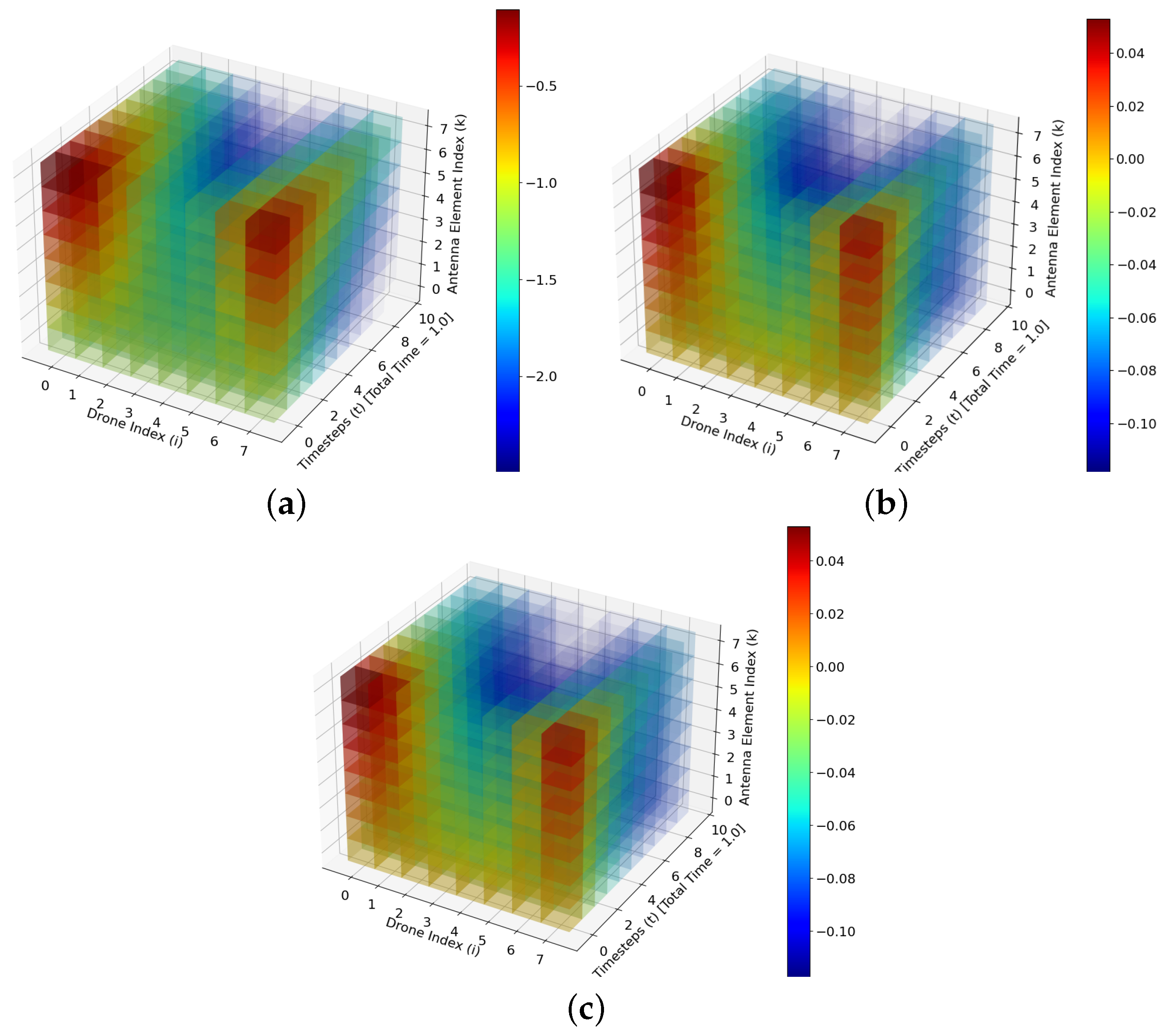
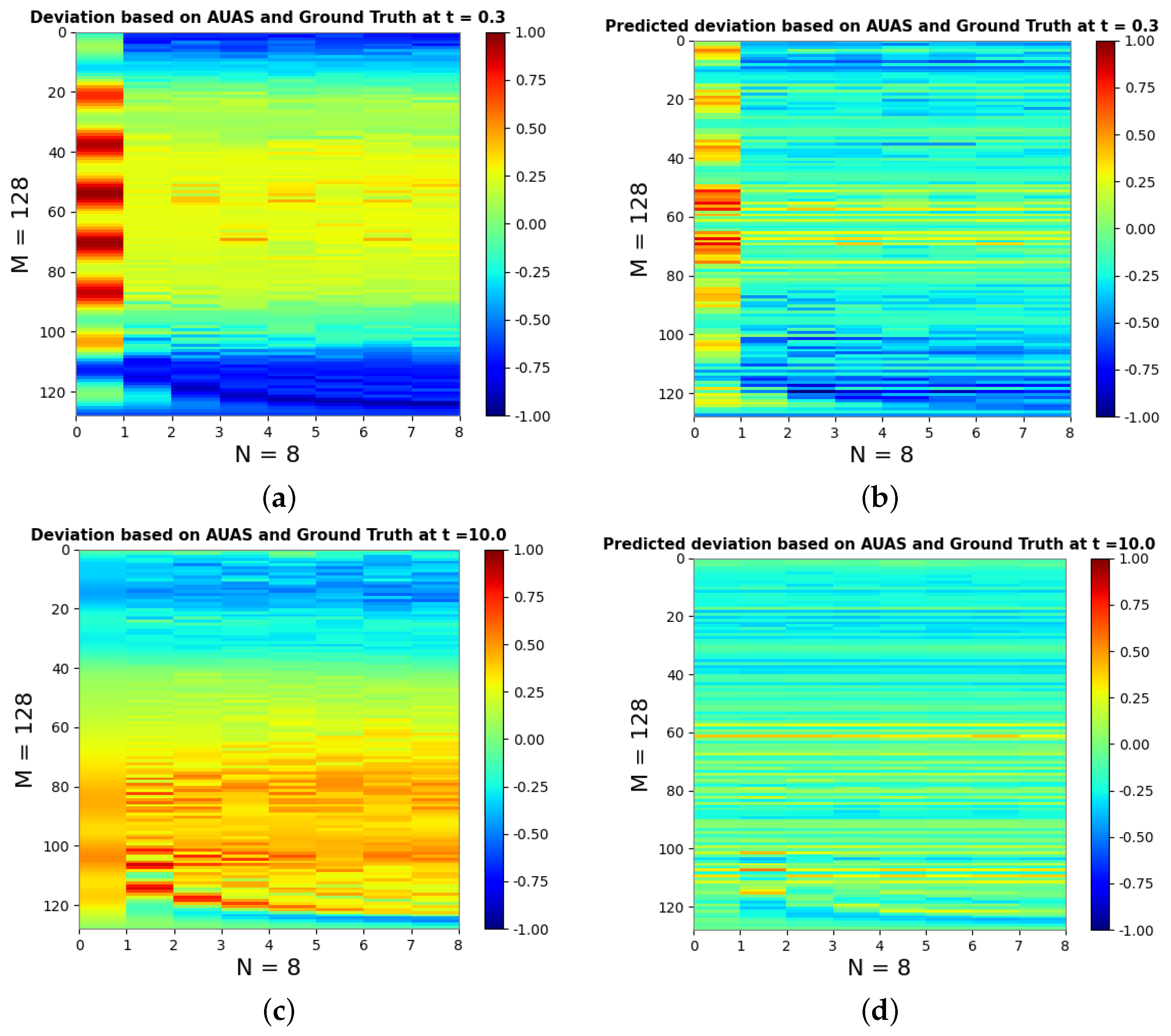
• In Section 3, we present time stamp simulations based on the proposed algorithm, i.e., the received beamformed signals of drones in the swarm at time stamps. Moreover, we compare the time-stamped beamformed signals corresponding to the proposed algorithm with the ground truth signals and the previous work to show the accuracy and compatibility of the algorithms.
• In Section 4, we present a feed-forward ANN based on the classical AUAS algorithm. The feed-forward ANN uses $3M+N$ inputs s.t. $\mathcal{O}\left(M\right)$ units and $\mathcal{O}\left(M^2\right)$ trainable parameters when $M\ge N$, to optimize the ML-based AUAS routing algorithm. We show that the optimization of the ML-based AUAS routing algorithm was achieved based on accuracy and efficiency.
• In Section 6, we conclude this paper.

We emphasize that the objective of this paper is to optimize the AUAS routing algorithm using a feed-forward neural network. The algorithm is different from AODV and OLSR, as it utilizes multi-beam beamforming to establish communication among drones. We do not address routing protocols for UAV networks based on topology, position, hierarchy, deterministic, stochastic, and social networks, as described in [57] and references therein. Also, we do not address sensors such as the electronic speed control and inertial measurement unit (an electromechanical device that consists of an accelerometer and a gyroscope) and controls such as proportional integral derivative control, adaptive control, localization and mapping methods, marker recognition algorithms, and vision-based schemes to route UAVs, as described in [58] and references therein.

2. Introducing Sparse Factors for the AUAS Model and a $\mathit{RSwarm}$ Routing Algorithm

In [1], we proposed a mathematical model to route a collection of AUAS consisting of over 100 members while answering the limitation of the existing AODV-based swarm members [59,60]. Continuing from the previous work, in this section, we present sparse factors for the mathematical model to reduce the complexity of the model in [1] and obtain a fast AUAS routing algorithm. The factorization is presented based on the frequency of Vandermonde matrices defined via spatiotemporal data. Before starting an AUAS routing algorithm, let us recall the mathematical model for routing drone swarms in [1].

2.1. Mathematical Model for AUAS Routing in [1]

We assumed a swarm consisting of M number of drones, and each drone—say u—has a uniform linear array with N elements and d element spacing. We also assumed that there are M uncorrelated signals impinging on the array from M drones (to establish communication among drones) with unique directions ${\left\{{\theta }_i\right\}}_{i=1}^M$, amplitudes ${\left\{a_i\right\}}_{i=1}^M$, and temporal variables ${\left\{{\omega }_i\right\}}_{i=1}^M$ s.t. $-2\pi f_i\le {\omega }_i<2\pi f_i$, where $f_i$ is the unique temporal frequency in each drone. These assumptions are made so that each drone could communicate using a unique RF beacon modulated at a low-rate digital waveform that carries a unique binary identification code and with no entering or leaving the drone in the drone swarm between deployment and landing. If ${\mathbf{x}}^{\left(u\right)}\left(t\right)={\left[x(0,t),x(1,t),\cdots ,x(M-1,t)\right]}^T$—say ${\mathbf{x}}^{\left(u\right)}$ denotes the source signal of drone u at time t, then the received N-beamformed signal of drone u at time t, i.e.,

$${\displaystyle {\mathbf{y}}^{\left(u\right)}({\omega }_i,a_i,{\theta }_i,t)=\sum _{k=0,i=1}^{N-1,M}{a}_i{e}^{j({\omega }_{i}t-k{\omega }_i{\psi }_i)}{\mathbf{x}}^{\left(u\right)}+{\mathbf{ȷ}}^{\left(u\right)},}$$

(1)

where ${\psi }_i=2\pi \frac{d}{\lambda }sin\left({\theta }_i\right)$, $\lambda$ denotes the wavelength of the incident signal, and ${\mathbf{ȷ}}^{\left(u\right)}\left(t\right)={\left[n_0\left(t\right),n_1\left(t\right),\cdots ,n_{N-1}\left(t\right)\right]}^T$—say ${\mathbf{ȷ}}^{\left(u\right)}$ is the Additive White Gaussian Noise (AWGN), takes the vector form ${\mathbf{y}}^{\left(u\right)}({\omega }_i,a_i,{\theta }_i,t)={\left[y(0,t),y(1,t),\cdots ,y(N-1,t)\right]}^T$—referred to as ${\mathbf{y}}^{\left(u\right)}$. Now, for all u’s, we can rewrite ${\mathbf{y}}^{\left(u\right)}$’s as a collection of matrix-vector products describing a MIMO beamforming model, and for each drone, u, described via:

$${\mathbf{y}}^{\left(u\right)}={\mathbf{V}}_{ki}^{\left(u\right)}·{\mathbf{S}}_i^{\left(u\right)}·{\mathbf{x}}^{\left(u\right)}+{\mathbf{ȷ}}^{\left(u\right)},$$

(2)

where ${\mathbf{V}}_{ki}^{\left(u\right)}={\left[e^{-jk{\omega }_i{\psi }_i}\right]}_{k=0,i=1}^{N-1,M}$ is an $N\times M$ matrix determined by spatial and temporal frequencies of each drone u, which is the frequency Vandermonde matrix (we recall here that such frequency Vandemonde matrices are a superclass of discrete Fourier transform matrices, and could be utilized to realize wideband multibeam beamforming, see [11,12,13,14]), $j^2=-1$, and ${\mathbf{S}}_i^{\left(u\right)}={\left[a_i{e}^{j{\omega }_{i}t}\right]}_{i=1}^M$ is an $M\times M$ matrix consisting of temporal frequencies and amplitudes. Thus, we will have a set of M systems of equations, and for each drone u, we have a system of N equations, i.e., a total of $MN$ equations in (2).

2.2. An Efficient AUAS Routing Algorithm, i.e., RSwarm Algorithm

This section presents a sparse factorization for frequency Vandermonde matrices determined by the spatiotemporal data of the drone swarm, and hence proposes an efficient classical algorithm to route a collection of AUAS. Before starting the factorization, let us take ${\delta }_i=e^{-j{\omega }_i{\psi }_i}$ for each drone $i=1,2,\cdots ,M$ corresponding to the nodes of the frequency Vandermonde matrices ${\mathbf{V}}_{ki}^{\left(u\right)}={\left[e^{-jk{\omega }_i{\psi }_i}\right]}_{k=0,i=1}^{N-1,M}$

Proposition 1.

Let the $M\times M$ frequency Vandermonde matrix for the drone, u, be given via ${\mathbf{V}}^{\left(u\right)}$, and its nodes be defined via $\{{\delta }_1,{\delta }_2,\dots ,{\delta }_M\}\in \mathbb{C}$ s.t. ${\delta }_i=e^{-j{\omega }_i{\psi }_i}$ for drones $i=1,2,\cdots ,M$. Then, the frequency Vandermonde matrix can be factored into the product of bidiagonal matrices s.t.

$${\mathbf{V}}^{\left(u\right)}={\mathbf{L}}_1{\mathbf{L}}_2\cdots {\mathbf{L}}_{M-1}{\mathbf{U}}_{M-1}\cdots {\mathbf{U}}_2{\mathbf{U}}_1,$$

(3)

where

$$\begin{array}{c}{\mathbf{U}}_k=\hfill \\ \hfill \begin{array}{c}\left[\begin{array}{cccccc}{\mathbf{I}}_{M-k-1}& & & & & \\ & 1& & & & \\ & & {\delta }_{M-k}({\delta }_1-1)& 1& & \\ & & & {\delta }_{M-k}({\delta }_2-1)& 1& \\ & & & & \ddots & 1\\ & & & & & {\delta }_{M-k}({\delta }_k-1)\end{array}\right],\hfill \end{array}\end{array}$$

and

$${\mathbf{L}}_k=\left[\begin{array}{cccccc}{\mathbf{I}}_{M-k-1}& & & & & \\ & 1& & & & \\ & {\delta }_1& 1& & & \\ & & {\delta }_2& 1& & \\ & & & \ddots & \ddots & \\ & & & & {\delta }_k& 1\end{array}\right].$$

where $k=1,2,\cdots ,M-1$, $\mathbf{I}$ is the identity matrix, and the empty spaces represent zero entries of the matrices.

Proof. 

This follows immediately from [11,61], when nodes are defined via ${\delta }_i$.    □

By following the above factorization, we obtain the following simple routing algorithm, i.e., the RSwarm Algorithm 1, to route a collection of AUAS. In Section 2.3 and Section 2.4, we show that the proposed algorithm attains low arithmetic and time complexities. Furthermore, in Section 3, we show that the performance of the proposed algorithm is compatible with the mathematical model (2). Thus, we present the RSwarm algorithm to route M drones, with each drone having an antenna array with M elements. We note here that the output of the algorithm provides M-beamformed received signals for each drone u at time t, i.e., ${\mathbf{y}}^{\left(u\right)}({\omega }_i,a_i,{\theta }_i,t)$, where ${\mathbf{x}}^{\left(u\right)}\left(t\right)$ is the input of the algorithm denoting the source signal of drone u at time t.

Algorithm 1 RSwarm

Input: M$f_i$, and t. Output: ${\mathbf{y}}^{\left(1\right)},{\mathbf{y}}^{\left(2\right)},\cdots ,{\mathbf{y}}^{\left(M\right)}$. for $i=1$ to M   Obtain ${\theta }_i$, $a_i$, ${\omega }_i$, ${\psi }_i$   Set ${\delta }_i\leftarrow e^{-j{\omega }_i{\psi }_i}$ end for for $u=1$ to M   Obtain ${\mathbf{x}}^{\left(u\right)}$ at t end for for $u=1$ to M    for $i=1$ to M    Construct ${\mathbf{S}}_i^{\left(u\right)}$    ${\mathbf{s}}^{\left(u\right)}\leftarrow {\mathbf{S}}_i^{\left(u\right)}·{\mathbf{x}}^{\left(u\right)}$    end for  end for   Construct $\tilde{\mathbf{V}}[{\mathbf{s}}^{\left(u\right)},0_{2M-1}]$   Calculate $\tilde{\mathbf{V}}[:,1\dots M-1]$   for $i=0$ to $M-2$    for $k=0$ to $M-1$    if $k+i<(M-2)$     ${\tilde{\mathbf{V}}}_{k(i+1)}\leftarrow {\tilde{\mathbf{V}}}_{ki}$    elseif $k+i=(M-2)$     ${\tilde{\mathbf{V}}}_{k(i+1)}\leftarrow {\tilde{\mathbf{V}}}_{ki}+{\tilde{\mathbf{V}}}_{(k+1)i}$    elseif $k=M-1$     ${\tilde{\mathbf{V}}}_{k(i+1)}\leftarrow {\tilde{\mathbf{V}}}_{ki}·({\delta }_k-{\delta }_{(M-i-2)})$    else     ${\tilde{\mathbf{V}}}_{k(i+1)}\leftarrow {\tilde{\mathbf{V}}}_{ki}·({\delta }_k-{\delta }_{(M-i-2)})+{\tilde{\mathbf{V}}}_{(k+1)i}$    end if    end for i   end for k   Calculate $\tilde{\mathbf{V}}[:,M\dots 2M-1]$   for $i=M-1$ to $2M-2$    for $k=0$ to $M-1$    if $k\le (i-M+1)$     ${\tilde{\mathbf{V}}}_{k(i+1)}\leftarrow {\tilde{\mathbf{V}}}_{ki}$    else     ${\tilde{\mathbf{V}}}_{k(i+1)}\leftarrow {\tilde{\mathbf{V}}}_{(k-1)i}·{\delta }_{(k-i+M-2)}+{\tilde{\mathbf{V}}}_{ki}$    end if    end for i   end for k     ${\mathbf{y}}^{\left(u\right)}\leftarrow \tilde{\mathbf{V}}[:,2M-1]$ end foru return${\mathbf{y}}^{\left(1\right)},{\mathbf{y}}^{\left(2\right)},\cdots ,{\mathbf{y}}^{\left(M\right)}$

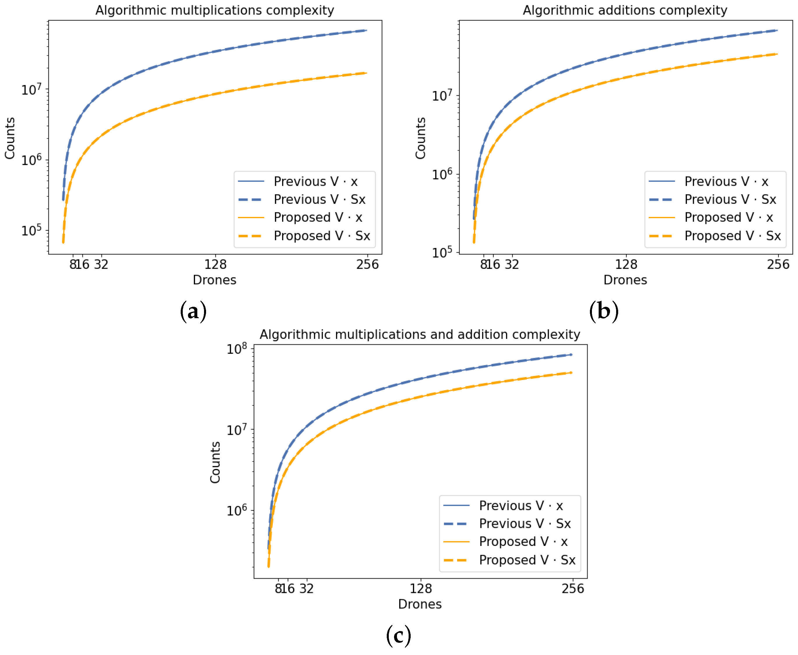
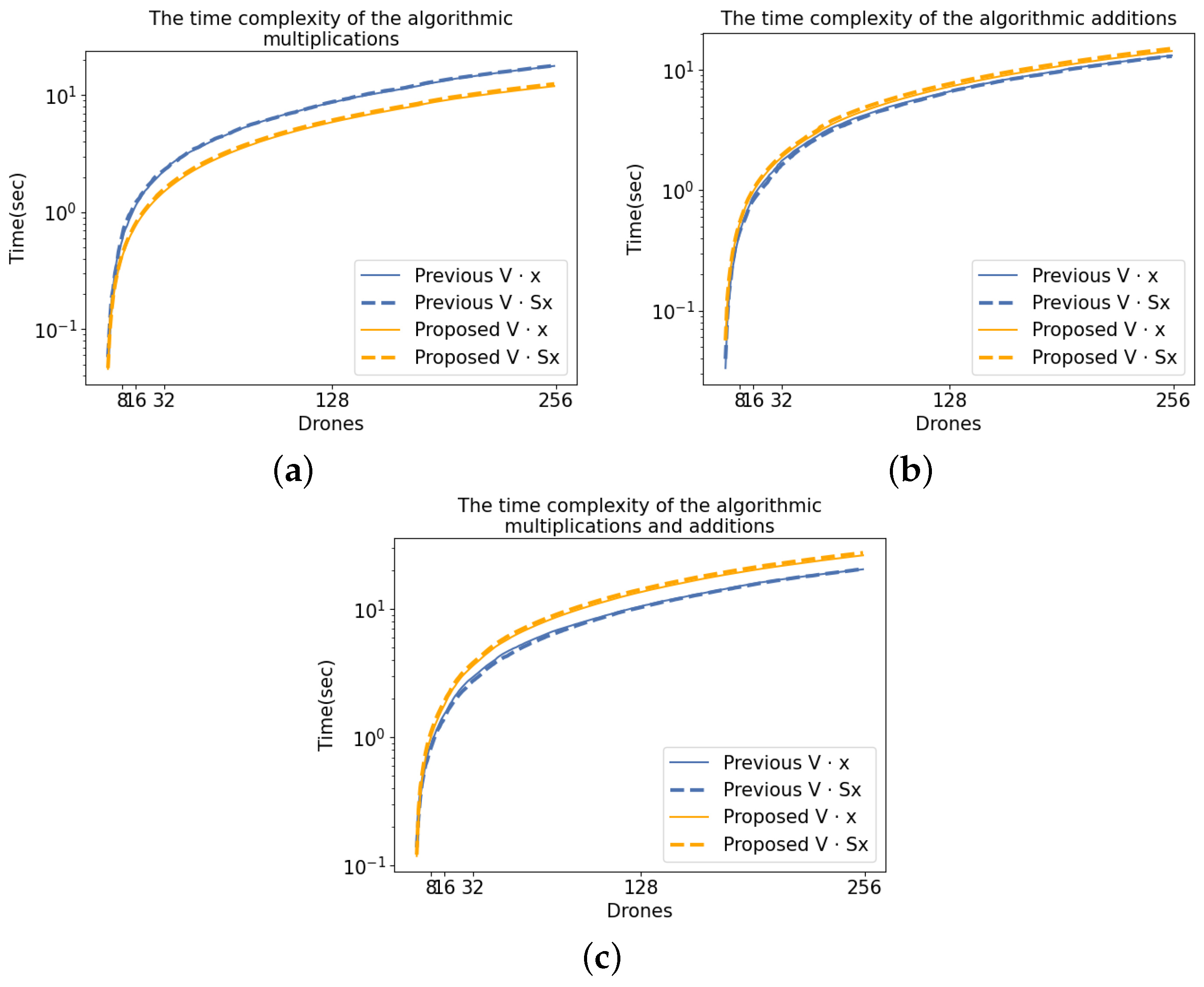
2.3. Arithmetic Complexity of the Algorithm

This section presents both the theoretical and numerical results in connection to the reduction in complexity, and hence shows the efficiency of the proposed routing algorithm. We recall here that particle swarm optimization has gained more attention as a stochastic optimization technique to route drone swarms. However, it does not consistently yield routing algorithms with low complexity [1,20,62]. On the other hand, the paper [63] shows the performance comparisons of particle swarm optimization and differential evolution techniques while identifying delivery routes, with minimal travel distances having quadratic complexity in both time and space. Nevertheless, this complexity has been computed based on a spatial distance matrix derived from the deployment to landing locations [1].

Here, we show that the RSwarm algorithm exhibits complexity that is less than quadratic. This advantage arises from the inherent property of the algorithm, wherein the value of N representing the number of elements in the antenna arrays remains constant after the deployment. Before establishing this, we obtain the arithmetic complexity of the proposed RSwarm algorithm, as follows.

Proposition 2.

The arithmetic complexity of the RSwarm routing algorithm having M number of drones and each drone consisting of a uniform linear array with N-elements, is $\mathcal{O}\left(N{M}^p\right)$, where p is less than the standard quadratic complexity.

Proof. 

We have M-sets of N-beamformed signals of M-drones, i.e., $[{\mathbf{y}}^{\left(1\right)},{\mathbf{y}}^{\left(2\right)},\cdots ,{\mathbf{y}}^{\left(M\right)}]$ as the columns of a throughput matrix to navigate the AUAS swarm. As each N-beamformed signal ${\mathbf{y}}^{\left(u\right)}$ correspondences to each drone described via (2) followed by the sparse factorization (3), the computation of the throughput matrix cost $\mathcal{O}\left(N{M}^p\right)$, where p is just about the quadratic power but less than the explicit quadratic complexity. □

Remark 1.

Since N is fixed after the deployment of the drone swarms, i.e., the number of elements in the antenna array is fixed after the deployments, and followed by the Proposition 2, the RSwarm algorithm has just less than the quadratic complexity, i.e., $\mathcal{O}\left(M^p\right)$, where $p<2$, while comparing with [1,20,62,63,64,65,66]. Furthermore, the RSwarm algorithm allows one to route a drone swarm with over 100 members, which is an improvement compared to the limitations of the existing AODV-based swarm members [15,59,60].

2.4. Numerical Results for the Arithmetic and Time Complexities of the Algorithm

In this section, we address numerical results based on the arithmetic and time complexities of the proposed routing algorithm. Moreover, the relationship between these complexities, along with the brute force calculation and the RSwarm algorithm, are illustrated in Figure 1 and Figure 2. These figures are drawn in the logarithmic scale representing the number of additions, number of multiplications, and timing required to execute the mathematical model based on the brute-force calculation vs. the RSwarm algorithms. The x-axis represents the number of drones, i.e., the number of elements in the antenna arrays (recall that M and N are the same), while the y-axis represents the arithmetic or time complexities. Referring to Figure 1, the algorithmic additions, multiplications, and their combination based on the RSwarm algorithm demonstrate the efficiency of the algorithm, as opposed to the brute-force calculation. Additionally, these results align with the theoretical complexity of the algorithm, i.e., the Proposition 2. Compared to the arithmetic complexity graphs in Figure 1, the time complexity graphs in Figure 2 do not show promising efficiency results of the RSwarm algorithm vs. the brute-force calculation. This discrepancy could be attributed to limitations in the processor speed and power. But, as expected, Figure 1 and Figure 2 show proportionality between time and arithmetic complexities. Moreover, both Figures also show that as the number of drones (also the number of elements in antenna arrays) increases, time and arithmetic complexities proportionally increase with that.

We note that the graphs in Figure 1 and Figure 2 do not demonstrate a significant improvement for a small number of drones or elements in the antenna arrays. However, they do show deviation as the number of drones or elements in the antenna arrays increases. This is because the RSwarm algorithm’s arithmetic (proportional time) complexities are not significantly affected by small values, but larger values experience a difference due to the proximity of the arithmetic and respective time complexity results.

Figure 1 and Figure 2 were generated using the Python code corresponding to the RSwarm algorithm. The timings were obtained using Python’s timeit module on a Lenovo Thinkpad X1 equipped with an Intel(R) Core(TM) i5-8265U CPU @ 1.60 GHz and 8 GB of RAM. The system was run with minimal concurrent applications.

3. Time-Stamp Simulations of the Algorithm

In this section, we present the received M-beamformed signals of each drone in the swarm at different time stamps, and assess the performance of the routing algorithm while comparing the performance with the output signals based on the previous work in [1] and ground truth signals.

We define the ground truth activation function as

$$\begin{array}{c}\hfill {\gamma }_{u,i,k}\left(t\right)=\sum _{u=1}^M\sum _{k=1}^N\left(\sum _{i=1}^{M}sin\left({\omega }_i·t+2\pi ·{\lambda }_i·{\beta }_{u,i,k}\right)\right)\end{array}$$

(4)

where ${\omega }_i$ is the temporal frequency of drone i, ${\lambda }_i$ is the spatial frequency of drone i, and ${\beta }_{u,i,k}$ is the distance from drone u’s kth antenna element to each antenna element of drone i at time t. In this simulation, ${\omega }_i=\frac{i·2\pi }{10}$ and ${\lambda }_i=\frac{1}{{\omega }_i}$, such that each drone is assigned a temporal and corresponding spatial frequency that is some multiple of the temporal frequency assigned to the drone with the slowest temporal frequency. This expresses what the sum of all waves emanating from each drone relative to drone u would look like from the view of drone u’s antenna array elements. In this way, the term “ground-truth” refers to the signal that would be experienced by any particular drone in the simulation. Comparing the output of this function for any given drone u and the output of the classical AUAS algorithm for a drone u is an important way to assess the ability of the classical AUAS model to map each drone’s M triplets of $\left[{\theta }^{\left(u\right)},a^{\left(u\right)},{\omega }^{\left(u\right)}\right]$ to an actual signal, and is also crucial for defining the training set for the post-processing FFANN designed to correct any deviation the AUAS algorithm output may have from the output it should have. Figure 3 shows M-beamformed signals corresponding to the antenna arrays in drones $1,2,...,M$ at time steps 0, 0.1, 0.2, …, 0.9., i.e., the values of the output signals ${\mathbf{y}}^{\left(u\right)}({\omega }_i,a_i,{\theta }_i,t)$, as u and i go from $1,2,...,M$. The color spectrum demonstrates the strength of the signal at time t per drone u at antenna element k. To generate Figure 3, we compare the activation function with the magnitude of the beamformed output vector multiplied by the sine value of the phase of the beamformed signals from all drones. This comparison considers spatial arrangements of drones at a specific time, experienced by each element of the antenna array. Following [1], we compare the ground truth signals with the output signals corresponding to the AUAS routing algorithm based on the following expression:

$$\sum _{i=1}^M\left|{\mathbf{y}}^{\left(u\right)}\right|·sin\left(arctan\left(\mathrm{Imag}({\mathbf{V}}_{ki}^{\left(u\right)}·{\mathbf{S}}_i^{\left(u\right)}·{\mathbf{x}}^{\left(u\right)}),\mathrm{Real}({\mathbf{V}}_{ki}^{\left(u\right)}·{\mathbf{S}}_i^{\left(u\right)}·{\mathbf{x}}^{\left(u\right)})\right)\right)$$

(5)

In Figure 3, the spatial arrangement of each drone is equally spaced along the circumference of a circle with a radius of 1 spatial unit. The angle $\alpha$ from the center of the circular formation to drone u is defined as ${\alpha }_i^{\left(u\right)}=\frac{2\pi }{M}i$, where the center of the formation is the origin, and each drone u is represented by spatial coordinates $\left(x^{\left(u\right)},y^{\left(u\right)}\right)=\left(cos{\alpha }^{\left(u\right)},sin{\alpha }^{\left(u\right)}\right)$. The amplitude of the received signal transmitted by drone i to drone u is set to $a_i^{\left(u\right)}=1$, and each drone’s linear M-element antenna array is horizontally oriented, with antenna k’s spatial coordinates of drone u represented as $\left(x^{\left(u\right)}+d\left(k-1\right),y^{\left(u\right)}\right)$, where $d=0.01$ represents the inter-element distance of the antenna arrays.

Figure 3 displays the M-beamformed signals (while color and transparency codes indicate the current amplitude of the signal, where negative amplitudes correspond to negative-valued sections of the real-valued representation of the signal) in antenna arrays of M drones (without a base station communication) at various time steps $t=0,0.1,0.2,...,0.9$. Here, ${\mathbf{y}}^{\left(u\right)}({\omega }_i,a_i,{\theta }_i,t)$ represent all combinations of u and i with $M=N=8$ and we compare the performance of the routing algorithm with the results in the paper [1] as well.

In Figure 3, each drone u in the circular spatial arrangement is depicted along the Drone Index axis, while its M-element antenna array is represented along the Antenna Element Index axis. It is important to note that this figure does not directly represent physical space; instead, it summarizes results from the perspective of multiple drones in a single figure, with each drone’s data stacked along the Drone Index axis.

The beamformed (output) signals of the RSwarm algorithm in Figure 3 demonstrate favorable results with the ground truth activation. As expected, the beamformed (output) signals obtained using the brute-force calculation of the model in [1] exhibited similar results to the RSwarm routing algorithm. This observation confirms that the adaptation of the sparse factorization to the frequency Vandermonde matrices followed by the RSwarm algorithm aligns precisely with the mathematical model in [1].

Figure 3 was generated using Python 3.10.12 using numpy 1.25 and matplotlib 3.7.1.

4. Optimize AUAS Routing Algorithm via ML

Feed-forward ANNs (FFANN) can improve the accuracy of the RSwarm algorithm by quantifying the performance of the ANN approximation, using measures like the loss and error. The FFANN plays a key role in optimizing the AUAS routing algorithm while reducing the error between the proposed algorithm and the ground truth signals, especially in having many drones with large numbers of elements in antenna arrays. The purpose of this FFANN during training is to interpret the output of the classical RSwarm algorithm and correct it to fit what would be expected given the signals being transmitted by other drones at their assigned frequencies and current orientations relative to a self drone. It does not predict drone locations directly; rather, it learns the relationship captured by the interference pattern between the RSwarm algorithm’s output and the ground truth signals at any given time. In deployment, this FFANN is inverted, transforming the raw sensory data from a linear beamforming array into the corresponding output from the classical RSwarm algorithm, which itself may be inverted to recover the distance and direction from a self-drone to all other drones in a swarm. This may then be used as a heuristic in many applications, including decentralized path-plotting and packet routing. This post-processing ANN will have the potential to significantly reduce the deviation from ground truth signals compared to our previous work on the error data in [1]. Thus, in this section, we will train parameters for the adaptive neural networks and hence obtain an optimized AUAS routing algorithm while reducing the error between the ML-based AUAS algorithm and the ground truth signals. This FFANN is implemented in Keras 2.10.0 backed by TensorFlow 2.10.1 and NVIDIA cuDNN 11.2.

To analyze the deviation of the received signals (based on the AUAS algorithm) from ground truth signals, we construct two data-sets based on the real components of the AUAS routing algorithm, ${\mathbf{y}}_{real}^{\left(u\right)}=\mathrm{Real}({\mathbf{V}}_{ki}^{\left(u\right)}·{\mathbf{S}}_i^{\left(u\right)}·{\mathbf{x}}^{\left(u\right)})$, as well as directions of incidents ${\left\{{\theta }_i\right\}}_{i=1}^M$, amplitudes ${\left\{a_i\right\}}_{i=1}^M$, and temporal variables ${\left\{{\omega }_i\right\}}_{i=1}^M$ in each drone $\forall u\in \{1,2,\dots ,M\}$.

The first-data set consists of data generation within the time interval from $t=0.0$ to $t=99.9$, with $0.1$ time steps. This data-set is generated according to the circular arrangement simulation described in Section 3, except the amplitude of the received signal of drone u from drone i is not assumed to be $a_i^{\left(u\right)}=1$, but is rather determined by an amplitude falloff function

$$\begin{array}{c}\hfill a_i^{\left(u\right)}=\frac{1}{{\left(1+d_i^{\left(u\right)}\right)}^2}\end{array}$$

(6)

where $d_i^{\left(u\right)}$ is the distance from transmitter drone i to receiver drone u.

The arrangement of the drone swarm in this first data-set guarantees that every drone receives a signal through its antenna array, with intricate interactions among each component signal. This specific case represented by the simulation scenario would be inadequate if the FFANN were predicting drone locations directly, since they are static and regularly structured. Since the FFANN is learning a relationship between wave patterns among a large number of waves over a long time period from every drone’s perspective, the scenario is sufficient as a proof-of-concept, since there is significant variety in the structure of the interference to test the feasibility of extracting a general relationship between the signal predicted by the classical RSwarm algorithm and the ground truth signals. This allows the post-processing ANN to demonstrate the generality without needing a large data set of random drone arrangements.

The second data-set (larger and more complex) consists of data generation with the time interval from $t=0.0$ to $t=99.9$ with $0.01$ time steps, also using the amplitude falloff function (6). This training set is generated according to a simulation, with drones traveling along deterministically generated and randomly assigned linear trajectories. The paths begin at $x_0^{\left(u\right)}$ and $y_0^{\left(u\right)}$ within the range $\left[-1,1\right]$ at $t=0$ and follow a path dictated by an angle ${\varphi }^{\left(u\right)}$ within the range $\left[0,2\pi \right)$. The function that computes a drone’s position $\left(x^{\left(u\right)},y^{\left(u\right)}\right)$ for any given t is stated as

$$\begin{array}{c}\hfill x^{(u,t)}=x_0^{\left(u\right)}+v·cos\left({\varphi }^{\left(u\right)}\right)·t\end{array}$$

(7)

and

$$\begin{array}{c}\hfill y^{(u,t)}=y_0^{\left(u\right)}+v·sin\left({\varphi }^{\left(u\right)}\right)·t\end{array}$$

(8)

where $x_0^{\left(u\right)}$ is the initial x-coordinate, $y_0^{\left(u\right)}$ is the initial y-coordinate, ${\varphi }^{\left(u\right)}$ is the direction angle, v is the rate of motion (set to $v=0.001$), and t is the time parameter. $x_0^{\left(u\right)}$, $y_0^{\left(u\right)}$, and ${\varphi }^{\left(u\right)}$ are all determined by a deterministic random process.

This simulation ensures that each drone receives a signal through its antenna array with intricate interactions between each signal. More general and representative real-world deployment situations would still be inadequate if the FFANN were predicting drone locations directly. This is because only a subset of all possible swarm trajectories are considered. As in the first scenario, the FFANN is learning a relationship between wave patterns among a large number of waves over a long time period from every drone’s perspective. But in the case of the second simulation, the origin points for these signals are randomized with non-static positions, which makes the scenario also sufficient as a proof-of-concept. As in the first simulation, there is significant variety in the structure of the interference to test the feasibility of extracting a general relationship between the signal predicted by the classical RSwarm algorithm and the ground truth signals. The second data-set allows the post-processing ANN to further demonstrate generality and flexibility with a larger, more complex data-set, allowing feasibility with real-world deployment scenarios.

Let us take each training input vector of the form

$${\tilde{\mathbf{x}}}^{(u,t)}:=\left[{\theta }_1^{\left(u\right)},a_1^{\left(u\right)},{\omega }_1^{\left(u\right)},\dots ,{\theta }_M^{\left(u\right)},a_M^{\left(u\right)},{\omega }_M^{\left(u\right)},y_1^{(u,t)},\dots ,y_N^{(u,t)}\right].$$

(9)

Recall from the mathematical model (2), followed by the RSwarm algorithm, that the training vectors ${\tilde{\mathbf{x}}}^{(u,t)}$ encompass various attributes including directions, amplitudes, and temporal frequencies. This comprehensive representation is important due to the multitude of potential source signal configurations, each corresponding to distinct ground-truth signals. By incorporating this information, the model is empowered to enhance its capacity to deduce instances in which ${\mathbf{y}}_{real}^{\left(u\right)}$ diverges from the ground-truth signals while avoiding reliance on the AUAS routing algorithm’s outputs. We note here that the variable t is not included explicitly in the input vectors, because the time variable is confined to being a seed value for generating signals within both the AUAS routing algorithm and ground-truth functions.

We consider each training output vector based on the deviation from ground truth and of the form,

$$\begin{array}{cc}\hfill {\tilde{\mathbf{y}}}^{(u,t)}& :=\mathrm{norm}\left(\left[{\tilde{y}}_1^{(u,t)},\dots ,{\tilde{y}}_N^{(u,t)}\right]\right)-\mathrm{norm}\left(\left[{\tilde{y}}_{1_{GT}}^{(u,t)},\dots ,{\tilde{y}}_{1_{GT}}^{(u,t)}\right]\right)\hfill \\ \hfill & =\left[{\tilde{y}}_{1_{dev}}^{(u,t)},\dots ,{\tilde{y}}_{N_{dev}}^{(u,t)}\right].\hfill \end{array}$$

(10)

where

$$\begin{array}{cc}\hfill & \mathrm{norm}\left(\left[{\tilde{y}}_1^{(u,t)},\dots ,{\tilde{y}}_N^{(u,t)}\right]\right)=\left[y^{\prime }({\tilde{y}}_1^{(u,t)},{\tilde{\mathbf{y}}}^{(u,t)}),\dots ,y^{\prime }({\tilde{y}}_N^{(u,t)},{\tilde{\mathbf{y}}}^{(u,t)})\right],\hfill \\ \hfill & \mathrm{norm}\left(\left[{\tilde{y}}_{1_{GT}}^{(u,t)},\dots ,{\tilde{y}}_{N_{GT}}^{(u,t)}\right]\right)=\left[y^{\prime }({\tilde{y}}_{1_{GT}}^{(u,t)},{\tilde{\mathbf{y}}}_{GT}^{(u,t)}),\dots ,y^{\prime }({\tilde{y}}_{N_{GT}}^{(u,t)},{\tilde{\mathbf{y}}}_{GT}^{(u,t)})\right],\hfill \end{array}$$

(11)

and

$$y^{\prime }\left(y,\tilde{\mathbf{v}}\right)=\frac{y-\min \left(\tilde{\mathbf{v}}\right)}{\max \left(\tilde{\mathbf{v}}\right)-\min \left(\tilde{\mathbf{v}}\right)}.$$

(12)

Given the dynamic movement of drones across different time stamps, and considering the diverse phase offsets, a strategic approach was adopted. Specifically, each ${\mathbf{y}}_{real}^{\left(u\right)}$ was incorporated within ${\tilde{\mathbf{x}}}^{(u,t)}$. Consequently, for each training instance ${\mathbf{y}}_{real}^{\left(u\right)}$ within ${\tilde{\mathbf{x}}}^{(u,t)}$, and each training instance ${\tilde{\mathbf{y}}}^{(u,t)}$, an individualized min-max normalization is applied using $y^{\prime }$, where y represents a scalar value within either ${\mathbf{y}}_{real}^{\left(u\right)}$ or ${\tilde{\mathbf{y}}}^{(u,t)}$, $\tilde{\mathbf{v}}$ is the vector ${\mathbf{y}}_{real}^{\left(u\right)}$ or ${\tilde{\mathbf{y}}}^{(u,t)}$, $\min \left(\tilde{\mathbf{v}}\right)$ is the minimum scalar value in $\tilde{\mathbf{v}}$, and $\max \left(\tilde{\mathbf{v}}\right)$ is the maximum scalar value in $\tilde{\mathbf{v}}$. Each instance of ${\tilde{\mathbf{x}}}^{(u,t)}$ contains an instance of ${\mathbf{y}}_{real}^{\left(u\right)}$ and each ${\tilde{\mathbf{y}}}^{(u,t)}$ is an instance of the deviation vector $\left[{\tilde{y}}_{1_{dev}}^{(u,t)},\dots ,{\tilde{y}}_{N_{dev}}^{(u,t)}\right]$. Each instance exhibits a distinct range, of which many are collectively depicted on each heatmap. The deviation from the ground signals with the visualization could be observed in terms of noise data, as illustrated in Figure 4.

The validation data-sets for both simulation scenarios are selected by allocating 10% of the generated data for validation purposes. Each validation sample ${\tilde{\mathbf{x}}}^{(u,t)}$ is chosen at random from the entire data-set, meaning each instance of ${\tilde{\mathbf{x}}}^{(u,t)}$ is chosen using random values of both t and u. This selection process ensures that the validation data effectively mirrors the network’s capacity to capture the interplay between the ground truth signals and the ML-based AUAS routing algorithm within the scope of our simulation scenarios. In larger, more comprehensive simulations, the range of potential relationships is significantly vast. However, the successful signal correction generalization within these simulations indicates that the performance may be comparable to the random case with a large, unbiased dataset. Given that our data exhibit interdependencies among incident signals that remain unaccounted for within our limited-scale data-sets, adopting an approach like selecting the final 10% of the time series as a contiguous segment would not yield a meaningful assessment of the network’s proficiency in showing the relationship between the output signals ${\mathbf{y}}_{real}^{\left(u\right)}$ and ground-truth signals in our simulations.

The FFANN model has 5 fully connected hidden layers with $\frac{3M+N}{2}$ units per layer. The number of elements in the network input vectors $|{\tilde{\mathbf{x}}}^{(u,t)}|=3M+N$, since there are M triplets of $\left[{\theta }^{\left(u\right)},a^{\left(u\right)},{\omega }^{\left(u\right)}\right]$ in every instance of ${\tilde{\mathbf{x}}}^{(u,t)}$, i.e., $\left[{\theta }_1^{\left(u\right)},a_1^{\left(u\right)},{\omega }_1^{\left(u\right)},\dots ,{\theta }_M^{\left(u\right)},a_M^{\left(u\right)}\right]$, as well as an instance of ${\mathbf{y}}_{real}^{\left(u\right)}$ with $|{\mathbf{y}}_{real}^{\left(u\right)}|=N$ elements. Empirically, halving this number yielded an acceptable performance, but further hyperparameter tuning may uncover a more precise scaling expression for the number of hidden units per layer. As mentioned in Section 4, we harness the swish activation in every layer except the linearly-activated output layer s.t.

$$\mathrm{swish}\left(x\right)=x·\frac{1}{1+exp(-\beta x)},$$

(13)

where $\beta$ is a learned parameter. Swish was chosen empirically due to exceeding the performance of networks that used ReLU, LeakyReLU, sigmoid, and tanh for their hidden layers. This may be due to the inherently smooth and non-linear nature of the problem of correcting a waveform. Thus, activation functions such as ReLU and LeakyReLU may be inappropriate due to their sharp transitions and linear behavior for positive inputs [67,68], and sigmoid and tanh may be less than ideal due to the vanishing-gradient problem [68,69]. Swish is by nature smooth, unlike ReLU and LeakyReLU, and does not suffer from the vanishing gradient problem to the same extent as sigmoid and tanh [68]. $l_2$ regularization was tested with the constant $\lambda$ setting to $0.0001$, $0.001$, and $0.01$, but all of these cases degraded the model performance significantly. Thus, $l_2$ regularization was not used. Batch normalization was used on all hidden layers except the final hidden layer to improve the model performance and reduce the training time.

Figure 4 depicts the model performance at $t=0.3$ and $t=10.0$. By predicting the deviation of the output of the classical RSwarm AUAS routing algorithm from the signal that is expected per the results of a physical simulation, the deviation may be removed. Thus, when the FFANN is inverted, the signal sensed by the drone is used as input to the model, and the signal is mapped into a form that the inverse of the classical RSwarm routing algorithm may take as input and turn into M triplets of $\left[{\theta }^{\left(u\right)},a^{\left(u\right)},{\omega }^{\left(u\right)}\right]$; this serves as a heuristic vector for many path-plotting and packet-routing algorithms that could be implemented in the swarm. While the model does manage to capture the shape of the deviation, it struggles to match the desired magnitude.

The proposed RSwarm algorithm does not exhibit substantial accuracy when compared with the ground truth function, as depicted in Figure 4a,c and Figure 5a,c. One could observe a remarkable enhancement of the accuracy when employing the FFANN with the RSwarm algorithm and comparing it with the ground truth function in both simulation scenarios, as illustrated in Figure 4b,d and Figure 5b,d. As a result, the integration of the multibeam beamforming-based mathematical model followed by the RSwarm algorithm with the ML significantly enhances the accuracy in routing the drone swarm.

In Figure 6, the graphical representation is shown for each model loss centered around the RSwarm algorithm integrated with the FFANN. Here, the loss is depicted in terms of the mean-squared error (MSE), and the performance is quantified in terms of the mean-absolute error (MAE) via

$$\mathrm{MSE}=\frac{1}{n}\sum _{i=1}^n{(y_i-{\widehat{y}}_i)}^2$$

(14)

$$\mathrm{MAE}=\frac{1}{n}\sum _{i=1}^n|y_i-{\widehat{y}}_i|$$

(15)

where $y_i$ represents an element of the training vector ${\tilde{\mathbf{y}}}^{(u,t)}$, and ${\widehat{y}}_i$ represents the model prediction for the ith element of the model output vector ${\widehat{\tilde{\mathbf{y}}}}^{(\mathbf{u},\mathbf{t})}$.

This configuration includes 128 drones; each drone is equipped with 8-element antenna arrays. The training for the model based on the smaller data-set with static drone positions is spanned over 512 epochs and utilized the Adam optimizer with a batch size of 64, while the training for the model based on the larger data-set with dynamic drone positions is spanned over 96 epochs. The training was conducted for 512 and 96 epochs, respectively, because the loss between the training and validation sets began to diverge beyond this point for this architecture. This configuration empirically results in an acceptable performance, but it may be possible to increase the batch size while maintaining a high network performance with larger, more varied data-sets, since general patterns may be captured more effectively within individual batches. As evident from the visual representation in Figure 6, the performance of the training process exhibits a great improvement as the number of epochs advances, simultaneously leading to a substantial reduction in the validation set loss. This shows the efficacy of the RSwarm algorithm with the FFANN, i.e., the ML-based AUAS routing algorithm, demonstrating the ability to rectify predictions based on the training data. Furthermore, the consistent decrease in the loss over epochs signifies the convergence of the proposed model, in conjunction with the FFANN, towards an alignment with the ground truth values.

5. Discussion

The presented AUAS algorithm followed by FFANN is specifically tailored for training with a fixed number of drones denoted as M, each associated with pre-defined weights ${\left\{{\omega }_i\right\}}_{i=1}^M$. Through our training processes, we established that these models exhibit a degree of robustness in scenarios where certain drones experience failures. In the simulation scenario with static drone positions, this robustness is demonstrated by the spatial configuration of drones, wherein drones are located diametrically opposite to a given drone u and thus have a negligible impact on its deviation from the actual value, attributed to the amplitude falloff function (6). In the simulation scenario with dynamic drone movement, this robustness is demonstrated as various drones move in and out of range from other drones, again attributed to the amplitude falloff function. To enhance this robustness to drone failure within the model, a more extensive training data-set could be constructed, incorporating drones with randomly assigned amplitudes of 0 to represent drones that are non-functional or otherwise separated from the swarm.

Thus, we have defined a heuristic that exhibits distinct advantages over those used by AODV and OLSR. By feeding raw antenna array data into the inverse of the FFANN described, and feeding that output into the inverse of the classical RSwarm AUAS algorithm, a table of neighbors, including their distances and directions from any “self” drone, may be efficiently generated. This information may be used for packet routing or physical path-plotting (among other potential applications). This heuristic is passive and does not require packet-based route establishment nor maintenance; it also does not require the broadcasting of link-state information. By harnessing the intrinsic properties of beam-forming linear antenna arrays, an overhead associated with AODV and OLSR may be reduced.

Our simulation scenarios are computationally efficient (see Section 3 and Section 4). The implementation of FFANN effectively demonstrates the enhanced performance of the classical RSwarm algorithm. One could also construct and train on a data-set using simulations that involve non-linear trajectories, demonstrating their potential. Such a data-set would likely lead to the development of more versatile and potent models, as it would capture a broader range of relationships between the AUAS routing algorithm and the ground-truth function.

Our pre-processing scheme prioritizes speed and low complexity during training and inference. However, this may come at the cost of accuracy. By normalizing the ${\mathbf{y}}_{real}^{\left(u\right)}$ component of the network (output vector), input vectors ${\tilde{\mathbf{x}}}^{(u,t)}$, vectors $\left[{\tilde{y}}_1^{(u,t)},\dots ,{\tilde{y}}_N^{(u,t)}\right]$, and $\left[{\tilde{y}}_{1_{GT}}^{(u,t)},\dots ,{\tilde{y}}_{1_{GT}}^{(u,t)}\right]$ (used to compute $\left[{\tilde{y}}_{1_{dev}}^{(u,t)},\dots ,{\tilde{y}}_{N_{dev}}^{(u,t)}\right]$), the pre-processing inference in deployment is fast. This is because the procedure only normalizes one small vector without having to store any buffer of prior instances of ${\mathbf{y}}_{real}^{\left(u\right)}$. This scheme does not need to know the statistical distribution of all possible instances of each vector. This depends on how accurately the training data represents real-world deployment scenarios. To do this, either a simulation environment or a large-scale real-world data-set is needed.

When we normalize ${\mathbf{y}}_{real}^{\left(u\right)}$ and ${\mathbf{y}}_{GT}^{\left(u\right)}$ based on their entire distribution, the magnitudes of ${\mathbf{y}}_{real}^{\left(u\right)}$ and ${\mathbf{y}}_{GT}^{\left(u\right)}$ often end up being significantly different from each other. While the ranges of the distributions for ${\mathbf{y}}_{real}^{\left(u\right)}$ and ${\mathbf{y}}_{GT}^{\left(u\right)}$ differ, there is often a similarity in the relationships between individual antenna elements at a given point in time for both. The main focus is on the interrelationships that show the difference between the output of the ML-based AUAS algorithm and the actual signal. The ability of the post-processing ANN to observe these relationships should not be affected by significant differences in the “baseline” values of individual ${\mathbf{y}}_{real}^{\left(u\right)}$ and ${\mathbf{y}}_{GT}^{\left(u\right)}$. This verifies that the ANN needs a buffer of previous values to determine which magnitude is greater. Consequently, the network eventually produces consistently biased predictions, incorporating the averages of both high positive and low negative values in an almost unpredictable manner. Consequently, the predictive capability of the network diminishes significantly, resulting in a close-to-zero output value that lacks effectiveness. By implementing the pre-processing scheme detailed in Section 4, we can retain the structural features of the data (frequency and relative amplitude information from various received signals), while eliminating the significant variations in the "baseline" mean. This, in turn, enables us to effectively correct the output of the network and maintain its shape. This greatly improves the AUAS routing algorithm, making it more useful for tasks such as path plotting and packet routing. The functioning of these applications depends on the accurate arrangement of other drones in relation to the signal strength and direction, as perceived by the self-drone. Including a previous ${\mathbf{y}}_{real}^{\left(u\right)}$ history buffer in the input to the ANN might provide the network with sufficient context to deduce these significant differences in magnitude, consequently broadening the applicability to situations where relative ordering alone is insufficient. However, implementing this approach may result in increased computational complexity because of the buffer and potentially require extra units in the post-processing ANN.

In a deployment context, the correction model’s capacity to handle drones is inherently constrained to a maximum limit. However, leveraging transfer learning allows one to employ a model across a spectrum of drone quantities, up to a designated threshold $M_{max}$. It is worth noting that adapting a model for different values of M through fine-tuning is distinct from the concept of randomly assigning some $a_i$ values to 0. In this context, the manual consideration and configuration of ${\theta }_i$ and ${\omega }_i$ values, as well as the arrangement of drones with a negligible amplitude in the training ${\tilde{\mathbf{x}}}^{(u,t)}$ vector, become essential.

In the utilization of transfer learning, determining the optimal value for $M_{max}$ necessitates a judicious assessment of the trade-off between the additional training time and model size, weighed against the advantages of reusable models across swarms of varying sizes without requiring retraining. Elevated values of $M_{max}$ heighten the training duration and model complexity while permitting the deployment within swarms of sizes $<=M$. Conversely, smaller $M_{max}$ values expedite the training and lower inference computational costs, albeit accommodating only smaller swarms. The impact of each trade-off depends on the experimental evaluation.

To optimize inference efficiency without substantial overhead, one could use convolutions over a historical series of ${\mathbf{y}}_{real}^{\left(u\right)}$ values, rather than relying solely on instantaneous values. This strategy leverages the fixed spatial spacing between antenna elements, capturing a fragment of the temporal information due to the propagation delay. However, it is crucial to note that this temporal aspect is dependent upon the individual values of ${\theta }_i$ and ${\omega }_i$ for each incident wave, thus introducing complexities for the model to infer. By considering such historical data, the model gains insights into the temporal dependencies of ${\mathbf{y}}_{real}^{\left(u\right)}$ features, as well as their interconnections with each corresponding ${\theta }_i$ and ${\omega }_i$. The evaluation of the performance improvement achieved with this architecture still needs to be tested through experiments, which will likely be influenced by the size and nature of the training data set.

6. Conclusions

We presented a novel, efficient, and classical RSwarm algorithm to route a collection of Autonomous Unmanned Aerial Systems. Our approach is based on the factorization of the frequency of Vandermonde matrices containing spatiotemporal data. We addressed time and arithmetic complexities, demonstrating their proportionality. Compared to brute-force calculations, the proposed algorithm exhibits low arithmetic and time complexities. We showed numerical simulations based on the beamformed signals of the proposed algorithm and compared that with ground truth signals. Finally, we presented an ML-based AUAS routing algorithm by combining the classical RSwarm routing algorithm with a feed-forward neural network. We compared the numerical results of the ML-based AUAS algorithm with the ground truth signals to demonstrate the accuracy of the proposed ML-based AUAS algorithm. The presented ML-based AUAS algorithm is a numerically accurate and scalable routing algorithm for a large-scale deployment.

References

1. Perera, S.M.; Myers, R.J.; Sullivan, K.; Byassee, K.; Song, H.; Madanayake, A. Integrating Communication and Sensor Arrays to Model and Navigate Autonomous Unmanned Aerial Systems. Electronics 2022, 11, 3023. [Google Scholar] [CrossRef]
2. Agiwal, M.; Roy, A.; Saxena, N. Next Generation 5G Wireless Networks: A Comprehensive Survey. IEEE Commun. Surv. Tutorials 2016, 18, 1617–1655. [Google Scholar] [CrossRef]
3. Lin, Z.; Lin, M.; de Cola, T.; Wang, J.B.; Zhu, W.P.; Cheng, J. Supporting IoT With Rate-Splitting Multiple Access in Satellite and Aerial-Integrated Networks. IEEE Internet Things J. 2021, 8, 11123–11134. [Google Scholar] [CrossRef]
4. Lin, Z.; Niu, H.; An, K.; Wang, Y.; Zheng, G.; Chatzinotas, S.; Hu, Y. Refracting RIS-Aided Hybrid Satellite-Terrestrial Relay Networks: Joint Beamforming Design and Optimization. IEEE Trans. Aerosp. Electron. Syst. 2022, 58, 3717–3724. [Google Scholar] [CrossRef]
5. Huang, Q.; Lin, M.; Wang, J.B.; Tsiftsis, T.A.; Wang, J. Energy Efficient Beamforming Schemes for Satellite-Aerial-Terrestrial Networks. IEEE Trans. Commun. 2020, 68, 3863–3875. [Google Scholar] [CrossRef]
6. Lin, Z.; Lin, M.; Zhu, W.P.; Wang, J.B.; Cheng, J. Robust Secure Beamforming for Wireless Powered Cognitive Satellite-Terrestrial Networks. IEEE Trans. Cogn. Commun. Netw. 2021, 7, 567–580. [Google Scholar] [CrossRef]
7. An, K.; Liang, T. Hybrid Satellite-Terrestrial Relay Networks with Adaptive Transmission. IEEE Trans. Veh. Technol. 2019, 68, 12448–12452. [Google Scholar] [CrossRef]
8. Jia, M.; Zhang, X.; Gu, X.; Guo, Q.; Li, Y.; Lin, P. Interbeam Interference Constrained Resource Allocation for Shared Spectrum Multibeam Satellite Communication Systems. IEEE Internet Things J. 2019, 6, 6052–6059. [Google Scholar] [CrossRef]
9. Li, B.; Fei, Z.; Chu, Z.; Zhou, F.; Wong, K.K.; Xiao, P. Robust Chance-Constrained Secure Transmission for Cognitive Satellite–Terrestrial Networks. IEEE Trans. Veh. Technol. 2018, 67, 4208–4219. [Google Scholar] [CrossRef]
10. Du, J.; Jiang, C.; Zhang, H.; Wang, X.; Ren, Y.; Debbah, M. Secure Satellite-Terrestrial Transmission Over Incumbent Terrestrial Networks via Cooperative Beamforming. IEEE J. Sel. Areas Commun. 2018, 36, 1367–1382. [Google Scholar] [CrossRef]
11. Perera, S.; Ariyarathna, V.; Udayanga, N.; Madanayake, A.; Wu, G.; Belostotski, L.; Cintra, R.; Rappaport, T. Wideband N-beam Arrays with Low-Complexity Algorithms and Mixed-Signal Integrated Circuits. IEEE J. Sel. Top. Signal Process. 2018, 12, 368–382. [Google Scholar] [CrossRef]
12. Perera, S.M.; Madanayake, A.; Cintra, R. Efficient and Self-Recursive Delay Vandermonde Algorithm for Multi-beam Antenna Arrays. IEEE Open J. Signal Process. 2020, 1, 64–76. [Google Scholar] [CrossRef]
13. Perera, S.M.; Madanayake, A.; Cintra, R. Radix-2 Self-recursive Algorithms for Vandermonde-type Matrices and True-Time-Delay Multi-Beam Antenna Arrays. IEEE Access 2020, 8, 25498–25508. [Google Scholar] [CrossRef]
14. Perera, S.M.; Lingsch, L.; Madanayake, A.; Mandal, S.; Mastronardi, N. Fast DVM Algorithm for Wideband Time-Delay Multi-Beam Beamformers. IEEE Trans. Signal Process. 2021, 70, 5913–5925. [Google Scholar] [CrossRef]
15. Huang, Y.; Wu, Q.; Wang, T.; Zhou, G.; Zhang, R. 3D Beam Tracking for Cellular-Connected UAV. IEEE Wirel. Commun. Lett. 2020, 9, 736–740. [Google Scholar] [CrossRef]
16. Di Caro, G.; Dorigo, M. AntNet: A Mobile Agents Approach to Adaptive Routing; Technical Report; IRIDIA: Carlsbad, CA, USA, 1997; pp. 97–112. [Google Scholar]
17. Di Caro, G.; Dorigo, M. AntNet: Distributed Stigmergetic Control for Communications Networks. J. Artif. Intell. Res. 1998, 9, 317–365. [Google Scholar] [CrossRef]
18. Mukhutdinov, D.; Filchenkov, A.; Shalyto, A.; Vyatkin, V. Multi-agent deep learning for simultaneous optimization for time and energy in distributed routing system. Future Gener. Comput. Syst. 2019, 94, 587–600. [Google Scholar] [CrossRef]
19. Caro, G.A.D.; Dorigo, M. Ant Colonies for Adaptive Routing in Packet-Switched Communications Networks. In Parallel Problem Solving from Nature; Springer: Berlin/Heidelberg, Germany, 1998. [Google Scholar]
20. Kassabalidis, I.; El-Sharkawi, M.; Marks, R.; Arabshahi, P.; Gray, A. Swarm Intelligence for Routing in Communication Networks. In Proceedings of the GLOBECOM’01—IEEE Global Telecommunications Conference (Cat. No. 01CH37270), San Antonio, TX, USA, 25–29 November 2001; Volume 6, pp. 3613–3617. [Google Scholar] [CrossRef]
21. Dhillon, S.S.; Van Mieghem, P. Performance Analysis of the AntNet Algorithm. Comput. Netw. 2007, 51, 2104–2125. [Google Scholar] [CrossRef]
22. Yang, X.; Li, Z.; Ge, X. Deployment Optimization of Multiple UAVs in Multi-UAV Assisted Cellular Networks. In Proceedings of the 2019 11th International Conference on Wireless Communications and Signal Processing (WCSP), Xi’an, China, 23–25 October 2019; pp. 1–7. [Google Scholar] [CrossRef]
23. Wang, J.; Liu, Y.; Amal, A.; Song, H.; Stansbury, R.S.; Yuan, J.; Yang, T. Fountain Code Enabled ADS-B for Aviation Security and Safety Enhancement. In Proceedings of the 2018 IEEE 37th International Performance Computing and Communications Conference (IPCCC), Orlando, FL, USA, 17–19 November 2018; pp. 1–7. [Google Scholar]
24. Leonov, A.V.; Litvinov, G.A. Applying AODV and OLSR routing protocols to air-to-air scenario in flying ad hoc networks formed by mini-UAVs. In Proceedings of the 2018 Systems of Signals Generating and Processing in the Field of on Board Communications, Moscow, Russia, 14–15 March 2018; pp. 1–10. [Google Scholar]
25. Messous, M.A.; Arfaoui, A.; Alioua, A.; Senouci, S.M. A Sequential Game Approach for Computation-Offloading in an UAV Network. In Proceedings of the GLOBECOM 2017—2017 IEEE Global Communications Conference, Singapore, 4–8 December 2017; pp. 1–7. [Google Scholar] [CrossRef]
26. Li, B.; Fei, Z.; Zhang, Y.; Guizani, M. Secure UAV Communication Networks over 5G. IEEE Wirel. Commun. 2019, 26, 114–120. [Google Scholar] [CrossRef]
27. Zhou, F.; Hu, R.Q.; Li, Z.; Wang, Y. Mobile Edge Computing in Unmanned Aerial Vehicle Networks. IEEE Wirel. Commun. 2020, 27, 140–146. [Google Scholar] [CrossRef]
28. Li, B.; Fei, Z.; Zhang, Y. UAV Communications for 5G and Beyond: Recent Advances and Future Trends. IEEE Internet Things J. 2019, 6, 2241–2263. [Google Scholar] [CrossRef]
29. Secinti, G.; Darian, P.B.; Canberk, B.; Chowdhury, K.R. SDNs in the Sky: Robust End-to-End Connectivity for Aerial Vehicular Networks. IEEE Commun. Mag. 2018, 56, 16–21. [Google Scholar] [CrossRef]
30. Sun, X.; Yang, W.; Cai, Y. Secure Communication in NOMA-Assisted Millimeter-Wave SWIPT UAV Networks. IEEE Internet Things J. 2020, 7, 1884–1897. [Google Scholar] [CrossRef]
31. Cui, J.; Liu, Y.; Nallanathan, A. The Application of Multi-Agent Reinforcement Learning in UAV Networks. In Proceedings of the 2019 IEEE International Conference on Communications Workshops (ICC Workshops), Shanghai, China, 20–24 May 2019; pp. 1–6. [Google Scholar] [CrossRef]
32. Zheng, K.; Sun, Y.; Lin, Z.; Tang, Y. UAV-assisted Online Video Downloading in Vehicular Networks: A Reinforcement Learning Approach. In Proceedings of the 2020 IEEE 91st Vehicular Technology Conference (VTC2020-Spring), Antwerp, Belgium, 25–28 May 2020; pp. 1–5. [Google Scholar] [CrossRef]
33. Chen, M.; Saad, W.; Yin, C. Liquid State Machine Learning for Resource and Cache Management in LTE-U Unmanned Aerial Vehicle (UAV) Networks. IEEE Trans. Wirel. Commun. 2019, 18, 1504–1517. [Google Scholar] [CrossRef]
34. Asif, N.A.; Sarker, Y.; Chakrabortty, R.K.; Ryan, M.J.; Ahamed, M.H.; Saha, D.K.; Badal, F.R.; Das, S.K.; Ali, M.F.; Moyeen, S.I.; et al. Graph Neural Network: A Comprehensive Review on Non-Euclidean Space. IEEE Access 2021, 9, 60588–60606. [Google Scholar] [CrossRef]
35. Sazli, M.H. A Brief Review of Feed-Forward Neural Networks. In Communications Faculty of Sciences University of Ankara Series A2-A3; Ankara University, Faculty of Engineering, Department of Electronics Engineering: Ankara, Turkey, 6 February 2006; Volume 50, pp. 11–17. [Google Scholar]
36. Hornik, K.; Stinchcombe, M.; White, H. Multilayer feedforward networks are universal approximators. Neural Netw. 1989, 2, 359–366. [Google Scholar] [CrossRef]
37. Wang, S.C. Artificial Neural Network. In Interdisciplinary Computing in Java Programming; Springer: Boston, MA, USA, 2003; pp. 81–100. [Google Scholar] [CrossRef]
38. Hornik, K. Approximation capabilities of multilayer feedforward networks. Neural Netw. 1991, 4, 251–257. [Google Scholar] [CrossRef]
39. Esmali Nojehdeh, M.; Aksoy, L.; Altun, M. Efficient Hardware Implementation of Artificial Neural Networks Using Approximate Multiply-Accumulate Blocks. In Proceedings of the 2020 IEEE Computer Society Annual Symposium on VLSI (ISVLSI), Limassol, Cyprus, 6–8 July 2020; pp. 96–101. [Google Scholar] [CrossRef]
40. Szegedy, C.; Zaremba, W.; Sutskever, I.; Bruna, J.; Erhan, D.; Goodfellow, I.J.; Fergus, R. Intriguing properties of neural networks. arXiv 2013, arXiv:1312.6199. [Google Scholar]
41. Tan, C.; Zhu, Y.; Guo, C. Building Verified Neural Networks with Specifications for Systems. In Proceedings of the 12th ACM SIGOPS Asia-Pacific Workshop on Systems; Association for Computing Machinery: New York, NY, USA, 2021; pp. 42–47. [Google Scholar]
42. Pennington, J.; Worah, P. Nonlinear random matrix theory for deep learning. In Proceedings of the 31st Conference on Neural Information Processing Systems (NIPS2017), Long Beach, CA, USA, 4–9 December 2017. [Google Scholar]
43. Baskerville, N.P.; Granziol, D.; Keating, J.P. Applicability of Random Matrix Theory in Deep Learning. arXiv 2021, arXiv:2102.06740. [Google Scholar]
44. Ghorbani, B.; Krishnan, S.; Xiao, Y. An Investigation into Neural Net Optimization via Hessian Eigenvalue Density. In Proceedings of the 36th International Conference on Machine Learning, Long Beach, CA, USA, 9–15 June 2019; Volume 97, pp. 2232–2241. [Google Scholar]
45. Dauphin, Y.N.; Pascanu, R.; Gulcehre, C.; Cho, K.; Ganguli, S.; Bengio, Y. Identifying and attacking the saddle point problem in high-dimensional non-convex optimization. In Proceedings of the Advances in Neural Information Processing Systems; Ghahramani, Z., Welling, M., Cortes, C., Lawrence, N., Weinberger, K., Eds.; Curran Associates, Inc.: Montreal, QC, Canada, 2014; Volume 27. [Google Scholar]
46. Verleysen, M.; Francois, D.; Simon, G.; Wertz, V. On the effects of dimensionality on data analysis with neural networks. In Proceedings of the Artificial Neural Nets Problem Solving Methods; Mira, J., Álvarez, J.R., Eds.; Springer: Berlin/Heidelberg, Germany, 2003; pp. 105–112. [Google Scholar]
47. Qin, L.; Gong, Y.; Tang, T.; Wang, Y.; Jin, J. Training Deep Nets with Progressive Batch Normalization on Multi-GPUs. Int. J. Parallel Program. 2018, 47, 373–387. [Google Scholar] [CrossRef]
48. Joshi, V.; Le Gallo, M.; Haefeli, S.; Boybat, I.; Nandakumar, S.R.; Piveteau, C.; Dazzi, M.; Rajendran, B.; Sebastian, A.; Eleftheriou, E. Accurate deep neural network inference using computational phase-change memory. Nat. Commun. 2020, 11, 2473. [Google Scholar] [CrossRef]
49. van de Ven, G.M.; Tuytelaars, T.; Tolias, A.S. Three types of incremental learning. Nat. Mach. Intell. 2022, 4, 1185–1197. [Google Scholar] [CrossRef]
50. Liu, Y.; Wang, J.; Li, J.; Niu, S.; Song, H. Class-Incremental Learning for Wireless Device Identification in IoT. IEEE Internet Things J. 2021, 8, 17227–17235. [Google Scholar] [CrossRef]
51. Liu, Y.; Wang, J.; Li, J.; Niu, S.; Wu, L.; Song, H. Zero-bias Deep Learning Enabled Quickest Abnormal Event Detection in IoT. IEEE Internet Things J. 2021, 9, 11385–11395. [Google Scholar] [CrossRef]
52. Zhou, M.; Wang, Q.; Shu, J.; Zhao, Q.; Meng, D. Diagnosing Batch Normalization in Class Incremental Learning. arXiv 2022, arXiv:2202.08025. [Google Scholar]
53. Liu, Y.; Wang, J.; Li, J.; Song, H.; Yang, T.; Niu, S.; Ming, Z. Zero-Bias Deep Learning for Accurate Identification of Internet-of-Things (IoT) Devices. IEEE Internet Things J. 2021, 8, 2627–2634. [Google Scholar] [CrossRef]
54. Garbin, C.; Zhu, X.; Marques, O. Dropout vs. batch normalization: An empirical study of their impact to deep learning. Multimed. Tools Appl. 2020, 79, 12777–12815. [Google Scholar] [CrossRef]
55. Dong, Y.; Ni, R.; Li, J.; Chen, Y.; Su, H.; Zhu, J. Stochastic Quantization for Learning Accurate Low-Bit Deep Neural Networks. Int. J. Comput. Vis. 2019, 127, 1629–1642. [Google Scholar] [CrossRef]
56. Ramachandran, P.; Zoph, B.; Le, Q.V. Searching for Activation Functions. arXiv 2017, arXiv:1710.05941. [Google Scholar]
57. Arafat, M.Y.; Moh, S. Routing Protocols for Unmanned Aerial Vehicle Networks: A Survey. IEEE Access 2019, 7, 99694–99720. [Google Scholar] [CrossRef]
58. Tahir, A.; Böling, J.M.; Haghbayan, M.H.; Toivonen, H.T.; Plosila, J. Swarms of Unmanned Aerial Vehicles—A Survey. J. Ind. Inf. Integr. 2019, 16, 100106. [Google Scholar] [CrossRef]
59. Wang, J.; Liu, Y.; Niu, S.; Song, H. 5G-enabled Optimal Bi-Throughput for UAS Swarm Networking. In Proceedings of the 2020 International Conference on Space-Air-Ground Computing (SAGC), Beijing, China, 4–6 December 2020; pp. 43–48. [Google Scholar] [CrossRef]
60. Wang, J.; Liu, Y.; Niu, S.; Song, H. Extensive Throughput Enhancement For 5G Enabled UAV Swarm Networking. IEEE J. Miniaturization Air Space Syst. 2021, 2, 199–208. [Google Scholar] [CrossRef]
61. Yang, S.L. On the LU factorization of the Vandermonde matrix. Discret. Appl. Math. 2005, 146, 102–105. [Google Scholar] [CrossRef]
62. Sohail, M.S.; Saeed, M.O.B.; Rizvi, S.Z.; Shoaib, M.; Sheikh, A.U.H. Low-Complexity Particle Swarm Optimization for Time-Critical Applications. arXiv 2014, arXiv:1401.0546. [Google Scholar]
63. Wisittipanich, W.; Phoungthong, K.; Srisuwannapa, C.; Baisukhan, A.; Wisittipanit, N. Performance Comparison between Particle Swarm Optimization and Differential Evolution Algorithms for Postman Delivery Routing Problem. Appl. Sci. 2021, 11, 2703. [Google Scholar] [CrossRef]
64. Chen, W.; Zhu, J.; Liu, J.; Guo, H. A fast coordination approach for large-scale drone swarm. J. Netw. Comput. Appl. 2024, 221, 103769. [Google Scholar] [CrossRef]
65. Javed, F.; Khan, H.Z.; Anjum, R. Communication capacity maximization in drone swarms. Drone Syst. Appl. 2023, 11, 1–12. [Google Scholar] [CrossRef]
66. Chen, Y.; Yang, D.; Yu, J. Multi-UAV Task Assignment With Parameter and Time-Sensitive Uncertainties Using Modified Two-Part Wolf Pack Search Algorithm. IEEE Trans. Aerosp. Electron. Syst. 2018, 54, 2853–2872. [Google Scholar] [CrossRef]
67. Huang, C. ReLU Networks Are Universal Approximators via Piecewise Linear or Constant Functions. Neural Comput. 2020, 32, 2249–2278. [Google Scholar] [CrossRef]
68. Szandała, T. Review and Comparison of Commonly Used Activation Functions for Deep Neural Networks. In Bio-Inspired Neurocomputing; Bhoi, A.K., Mallick, P.K., Liu, C.M., Balas, V.E., Eds.; Springer: Singapore, 2021; pp. 203–224. [Google Scholar] [CrossRef]
69. Rumelhart, D.E.; Hinton, G.E.; Williams, R.J. Learning representations by back-propagating errors. Nature 1986, 323, 533–536. [Google Scholar] [CrossRef]
Figure 1. Based on the execution of the proposed algorithm and brute-force mathematical model, followed by the codes written in Python and the timeit module: (a) shows the log-scaled number of multiplications, (b) shows the log-scaled number of additions, and (c) shows the log-scaled number of additions and multiplications.
Drones 08 00057 g001
Figure 2. Based on the execution of the proposed algorithm and brute-force mathematical model, followed by the codes written in Python and the timeit module: (a) shows the log-scaled execution time corresponding to multiplications, (b) shows the log-scaled execution time corresponding to additions, and (c) shows the log-scaled execution time corresponding to additions and multiplications.
Drones 08 00057 g002
Figure 3. (a) illustrates the output of the ground truth activation function γ u , i , k t , (b) depicts the beamformed (output) signals of the mathematical model in [1], and (c) depicts the beamformed (output) signals of the RSwarm routing algorithm y ( u ) ( ω i , a i , θ i , t ) over 10 time steps with 0.1 per time step.
Drones 08 00057 g003
Figure 4. Depictions of the deviation of the RSwarm algorithm from ground truth signals, and predicted deviation from ground truth from the RSwarm algorithm by the static position simulation-derived FFANN model having 128 drones—each drone having eight element antenna arrays. (a) shows the deviation of the RSwarm algorithm with the ground truth at t = 0.3 in the static position scenario, (b) shows the predicted deviation based on the RSwarm algorithm with FFANN to ground truth at t = 0.3 in the static position scenario, (c) shows the deviation of RSwarm algorithm with the ground truth at t = 10.0 in the static position scenario, and (d) shows the predicted deviation based on the RSwarm algorithm with FFANN to the ground truth at t = 10.0 in the static position scenario.
Drones 08 00057 g004
Figure 5. Depictions of the deviation of the RSwarm algorithm from ground truth signals, and the predicted deviation of the RSwarm algorithm by the dynamic movement simulation-derived FFANN model from the ground truth with 128 drones; each drone had eight elements of antenna arrays. (a) shows the deviation of the RSwarm algorithm with the ground truth at t = 0.3 in the dynamic position scenario, (b) shows the predicted deviation based on the RSwarm algorithm with FFANN in the ground truth at t = 0.3 in the dynamic position scenario, (c) shows the deviation of RSwarm algorithm with the ground truth at t = 10.0 in the dynamic position scenario, and (d) shows the predicted deviation based on the RSwarm algorithm with FFANN in the ground truth at t = 10.0 in the dynamic position scenario. For clarity in the visual interpretation, the rows in the predicted deviation images are sorted such that each subsequent row is the closest in Euclidean distance to the preceding one by computing the pairwise Euclidean distances d i j = k ( x i k x j k ) 2 , where d i j represents the Euclidean distance between rows i and j, and x i k and x j k are the k−th components of rows i and j, respectively. The rows in (a,c) are ordered following the same row index sequence, ensuring that for any given row in the prediction depiction, the corresponding row in the target depiction matches it.
Drones 08 00057 g005
Figure 6. Model performance metrics’ mean-squared-error loss and mean-absolute error for each training epoch is shown here for each model, i.e., AUAS algorithm with FFANN for both simulations, having 128 drones, each with 8-element antenna arrays. (a) shows mean-squared-error loss for the static position simulation-derived model, (b) shows mean-absolute-error for the static position simulation-derived model, (c) shows mean-squared-error loss for the dynamic motion simulation-derived model, and (d) shows mean-absolute-error for the dynamic motion simulation-derived model.
Drones 08 00057 g006
Disclaimer/Publisher’s Note: The statements, opinions and data contained in all publications are solely those of the individual author(s) and contributor(s) and not of MDPI and/or the editor(s). MDPI and/or the editor(s) disclaim responsibility for any injury to people or property resulting from any ideas, methods, instructions or products referred to in the content.