Coverage Path Planning for UAVs: An Energy-Efficient Method in Convex and Non-Convex Mixed Regions

Abstract

As an important branch of path planning, coverage path planning (CPP) is widely used for unmanned aerial vehicles (UAVs) to cover target regions with lower energy consumption. Most current works focus on convex regions, whereas others need pre-decomposition to deal with non-convex or mixed regions. Therefore, it is necessary to pursue a concise and efficient method for the latter. This paper proposes a two-stage method named Shrink-Segment by Dynamic Programming (SSDP), which aims to cover mixed regions with limited energy. First, instead of decomposing and then planning, SSDP formulates an optimal path by shrinking the rings for mixed regions. Second, a dynamic programming (DP)-based approach is used to segment the overall path for UAVs in order to meet energy limits. Experimental results show that the proposed method achieves less path overlap and lower energy consumption compared to state-of-the-art methods.

1. Introduction

Unmanned aerial vehicles (UAVs) have become widely used in applications such as aerial photography [1] and rescue [2,3,4]. Due to restrictions on permitted flight regions and battery capacity, there has been extensive research on UAV path planning [5,6,7]. Coverage path planning (CPP) is a critical subset of UAV path planning. The primary challenge lies in designing feasible routes for UAVs within target regions to ensure thorough coverage of the entire space while optimizing energy consumption. Key objectives include minimizing redundant coverage, avoiding collisions between UAVs, and achieving specific tasks such as monitoring crop conditions or detecting targets.

Most existing approaches to CPP focus on obstacle avoidance [8,9,10], region decomposition [11,12], energy consumption [13,14], and UAV collaboration [15,16]. The methods for covering a region in these studies can be broadly categorized into two patterns, namely, back-and-forth (B&F) and spiral. Mu et al. [8] introduced the continuity constraint function within B&F to reduce coverage overlap. Nielsen et al. [11] showed that the travel direction in B&F should be aligned vertically relative to the shortest edge of the polygon. Cabreira et al. [13] proposed a spiral coverage method and optimized the speed along straight segments to minimize energy consumption. However, these methods are only suited for convex polygons; when applied to non-convex polygons, region decomposition is required. For example, Choset et al. [9] used a sweep line to partition regions, and Nielsen et al. [11] extended the edges of concave angles to decompose non-convex regions.

The studies mentioned above focused solely on single-region scenarios; however, in tasks such as disaster relief, the presence of rivers and mountains often leads to the division of the target area into several smaller regions. Using UAVs to cover multiple regions is generally divided into two steps: determining the regional access order, and determining the path within each region. The first step is similar to the traveling salesman problem (TSP). Based on this, Vasquez-Gomez et al. [17] proposed a two-step method called TSPP. First, TSPP estimates the cost using the distance between the centroids of polygons and applies a genetic algorithm (GA) to determine the visiting order. Second, it computes the B&F paths for each region based on this order. Xiao et al. [18] proposed a clustering algorithm called CSCA to assign regions to UAVs. In CSCA, UAV starting points are initialized as cluster centers. By adding regions to the clusters and updating them, each UAV is assigned at least one region. Then, the nearest-to-end policy and B&F pattern are used to determine the regional access order and intra-region paths. Du et al. [19] proposed a method that mixes B&F and spiral paths to ensure complete coverage of regions. In this method, the B&F path is generated by dividing the polygon into multiple strips based on the sensor’s width, while the spiral path is created using the perpendicular bisectors of the polygon’s edges. However, these algorithms only address energy consumption in the results, and do not take into account the constraints imposed by the drone’s battery capacity.

In fact, the energy constraint should be included in the problem’s assumptions. Xie et al. [20] defined the problem as an energy-constrained multiple TSP-CPP (EMTSP-CPP). This EMTSP-CPP requires the UAVs to collaboratively complete the coverage task under limited energy, with each UAV departing from the warehouse and returning after completing its task. Xie et al. used a GA combined with grouping to assign regions to each UAV. To achieve a similar objective, Ahmed et al. [21] employed a greedy algorithm integrated with a heuristic approach. Jiang et al. [22] used an improved fuzzy c-means clustering algorithm to assign regions, but did not account for intra-region paths. Unfortunately, the coverage paths resulting from these methods are not optimal. For one, if a UAV finishes covering a region and is closer to the next region than to its starting point, it should continue to the next region if it has enough energy. In addition, a single UAV may not be able to cover a large region of interest on its own. To address these issues, Luna et al. [23] proposed the BINPAT algorithm, which first designs a globally optimal coverage path and then divides it among the UAVs. Compared to regional division, route division considers UAV incorporation rather than merely ensuring that they do not interfere with each other. While BINPAT is implemented using the Jonker–Volgenant algorithm [24], its time complexity of $O\left(n^3\right)$ results in significant computational time when the number of waypoints is large. Furthermore, BINPAT simplifies the energy constraint to a distance constraint without accounting for the energy consumption caused by UAVs needing to make turns.

This paper aims to determine the optimal coverage paths for energy-constrained UAVs in convex and non-convex mixed regions. To achieve this goal, a two-stage method called Shrink-Segment by Dynamic Programming (SSDP) is proposed. In its first stage, SSDP uses a polygon offset-based shrink method to generate shrinking rings. With the objective of minimizing energy consumption, shrinking rings from each region are then connected sequentially from the outermost to the innermost, resulting in an optimal coverage path. In the second stage, a dynamic programming (DP)-based approach is used to segment the overall path for UAVs. The principal contributions of this research are as follows:

• A shrink method is proposed which is suitable for both convex and non-convex regions. This method reduces operational complexity is directly applicable to non-convex regions, thereby avoiding the need for pre-decomposition.
• A DP-based approach is proposed to optimally segment the overall path among UAVs, allowing some UAVs to remain on standby rather than adhering to the principle of equal or maximum load distribution.
• The proposed SSDP ensures that UAVs meet their respective energy constraints while minimizing overall energy consumption.

The remainder of this paper is organized as follows: the problem formulation and method overview are introduced in Section 2; Section 3 provides details on the shrink method, followed by the DP-based approach in Section 4; experimental results and discussion are presented in Section 5; finally, Section 6 presents our conclusion.

2. Problem Definition and Method Overview

This section employs mathematical symbols to describe the coverage path planning problem for UAVs. First, the inputs and outputs of the problem are defined. Second, the constraints are established to ensure the feasibility of path planning and comprehensive region coverage. Finally, the overall framework of the proposed SSDP method is outlined.

2.1. Problem Formulation

In this study, we deploy N homogeneous UAVs $\{u_n,n\in [1,N]\}$, which all start from a warehouse $w_0$, to scan M regions $\{{\mathit{R}}_m,m\in [1,M]\}$. Region ${\mathit{R}}_m=({\mathit{v}}_m^1,{\mathit{v}}_m^2,...,{\mathit{v}}_m^{r_m})$ can be of any type, either convex or non-convex, with ${\mathit{v}}_m^{r_m}=(x_m^{r_m},y_m^{r_m})$ indicating the coordinates of the $r_m$-th vertex. Here, $x_m^{r_m}$ and $y_m^{r_m}$ denote the horizontal and vertical coordinate, respectively. The number of vertices in each region is not fixed, with $r_m$ being determined case-by-case.

We assume that UAV $u_n$ flies at a constant speed V and has an energy constraint $E_n$. Because all UAVs are of the same type, their energy consumption is identical. Let $E=E_1=E_2=\cdots =E_n$ represent this common energy consumption. The sensor model of UAV is shown as Figure 1, where $L_1$ represents the longitudinal scanning length of the sensor camera; correspondingly, $L_2$ represents the lateral scanning length. To ensure thorough scanning of these target regions, it is required that the images captured by the UAVs have a certain overlap length, denoted as $L_1^{\prime }$ and $L_2^{\prime }$ for the longitudinal and lateral directions, respectively.

Each UAV is authorized to access all regions. Additionally, considering that the core objective of the coverage task is to obtain comprehensive ground data, the UAVs fly at a sufficient altitude, eliminating the need to avoid any obstacles.

The task result is to distribute a series of waypoints $\{{\mathit{W}}_n,n\in [1,N]\}$ to the UAV swarm that provides coordinated coverage of all target regions. In this context, ${\mathit{W}}_n=({\mathit{w}}_n^1,{\mathit{w}}_n^2,...,{\mathit{w}}_n^{k_n})$ represents the flight path for UAV $u_n$, with ${\mathit{w}}_n^{k_n}=(x_n^{k_n},y_n^{k_n})$ being the $k_n$-th waypoint.

2.2. Problem Constraints

This section analyzes the constraints that must be followed when UAVs cover mixed regions. Moreover, an optimization model is developed to enable the UAVs to complete the coverage task with minimal energy consumption.

Constraint 1 (C1): All UAVs are required to depart from the warehouse ${\mathit{w}}_0$ before executing their tasks and return to the warehouse upon completion. Therefore, ${\mathit{W}}_n=({\mathit{w}}_n^1,{\mathit{w}}_n^2,...,{\mathit{w}}_n^{k_n})$ must satisfy the following condition:

$$\forall n\in [1,N],{\mathit{w}}_n^1={\mathit{w}}_n^{k_n}={\mathit{w}}_0$$

(1)

where ${\mathit{w}}_n^1$ represents the first waypoint of UAV $u_n$ and ${\mathit{w}}_n^{k_n}$ represents its last waypoint.

Constraint 2 (C2): To ensure complete coverage, each region must be covered by at least one UAV. We define a variable $c_{n,m}$ to indicate whether $u_n$ is involved in the coverage of ${\mathit{R}}_m$. The value of $c_{n,m}$ is defined as shown below.

$$\exists {\mathit{w}}_n^i\in {\mathit{W}}_n,i\in [2,k_n-1],c_{n,m}=\left\{\begin{array}{cc}1,\hfill & {\mathit{w}}_n^i\mathrm{located}\mathrm{within}{\mathit{R}}_m\hfill \\ 0,\hfill & \mathrm{otherwise}\hfill \end{array}\right.$$

(2)

Furthermore, $c_{n,m}$ must satisfy the following condition:

$$\forall m\in [1,M],\sum _{n=1}^N{c}_{n,m}\ge 1.$$

(3)

Constraint 3 (C3): To avoid multiple coverage, a UAV can cover a maximum of M regions; thus, the variable $c_{n,m}$ must satisfy the following constraint:

$$\forall n\in [1,N],0\le \sum _{m=1}^M{c}_{n,m}\le M.$$

(4)

Constraint 4 (C4): Due to the maximum energy consumption E of the UAV, the waypoint set ${\mathit{W}}_n$ of $u_n$ must satisfy the following constraint:

$$\forall n\in [1,N],{\lambda }_1\times \sum _{i=1}^{k_n-1}\mathrm{d}({\mathit{w}}_n^i,{\mathit{w}}_n^{i+1})+{\lambda }_2\times \sum _{i=2}^{k_n-1}\mathrm{a}({\mathit{w}}_n^{i-1},{\mathit{w}}_n^i,{\mathit{w}}_n^{i+1})\le E$$

(5)

where ${\lambda }_1$ represents the weight of distance in energy consumption and ${\lambda }_2$ denotes the weight of turning in energy consumption; according to [25], the values of the coefficients ${\lambda }_1$ and ${\lambda }_2$ have been determined as 0.1072 and 0.0104, respectively. Additionally, $\mathrm{d}({\mathit{w}}_n^i,{\mathit{w}}_n^{i+1})$ represents the path distance for $u_n$ from ${\mathit{w}}_n^i$ to ${\mathit{w}}_n^{i+1}$, while $\mathrm{a}({\mathit{w}}_n^{i-1},{\mathit{w}}_n^i,{\mathit{w}}_n^{i+1})$ represents the turning angle for $u_n$ travels from ${\mathit{w}}_n^{i-1}$ through ${\mathit{w}}_n^i$ to ${\mathit{w}}_n^{i+1}$.

In this paper, we aim to plan a series of paths that allows the UAVs to cover these target regions while minimizing energy consumption as much as possible. The total energy consumption of the UAV swarm is determined by the sum of the path distances and the turning angles of each UAV, expressed as follows:

$$p={\lambda }_1\times \sum _{n=1}^N\sum _{i=1}^{k_n-1}\mathrm{d}({\mathit{w}}_n^i,{\mathit{w}}_n^{i+1})+{\lambda }_2\times \sum _{n=1}^N\sum _{i=2}^{k_n-1}\mathrm{a}({\mathit{w}}_n^{i-1},{\mathit{w}}_n^i,{\mathit{w}}_n^{i+1}).$$

(6)

Finally, the mission optimization process can be formulated as

$$\begin{array}{cc}\hfill \min & p\hfill \\ \hfill \mathrm{s}.\mathrm{t}.& \mathrm{C}1,\mathrm{C}2,\mathrm{C}3,\mathrm{C}4\hfill \end{array}$$

(7)

Calculating the Euclidean distance between waypoints is required in Equation (6). This introduces a nonlinear objective function, making it a nonlinear programming (NLP) problem. Furthermore, the selection of coverage paths involves combinatorial complexity. As the number of regions increases, the number of possible path combinations grows exponentially. Therefore, this problem is also classified as NP-hard, indicating high computational complexity.

2.3. Method Overview

We propose a two-stage method to address this problem, which we name SSDP. In the first stage, the shrink method generates an optimal coverage path through three steps: first, shrinking rings for each region are generated using the polygon offset method; second, the shrinking rings are broken into waypoints; and finally, these waypoints are connected to form the optimal coverage path. In the second stage, we employ a DP-based approach combining a two-dimensional matrix with memoization to segment the path into individual flight paths for the UAVs. The flowchart of SSDP is shown in Figure 2.

3. Optimal Coverage Path Generation

This section provides a detailed explanation of the first stage of SSDP. The core idea is to use iterative polygon offsetting operations to generate an optimal coverage path for all target regions, whether convex or non-convex. The following subsections discuss the principles of generating shrinking rings through polygon offset, strategies for evenly distributing waypoints, and methods for orderly connection of waypoints between rings. These steps lay a solid foundation for the subsequent path segmentation and allocation processes.

3.1. Shrinking Ring Generation

First, we take the boundary of the region as the initial shrinking ring. Using the polygon offset method, the first ring is shifted inward by a distance of $L_1$–$L_1^{\prime }$ to generate the second shrinking ring. The same method is then applied to generate the third shrinking ring. In certain cases, offsetting the previous shrinking ring may result in multiple new shrinking rings. We use a depth-first search strategy to continue generating these rings. The search process continues until a UAV flying along a specific shrinking ring can fully observe all of the information within the ring, at which point that shrinking ring is considered the final one.

The polygon offset method we employ here is our improvement of the work by Lee et al. [26]. The polygon offset method generates offset vertices by using the vertices of the previous shrinking ring and organizes them into an offset vertex list $\mathit{OVL}$. Next, adjacent offset vertices in $\mathit{OVL}$ are connected to form offset edges, which are then organized into an offset edge list $\mathit{OEL}$. By comparing the directional and positional information, each offset edge is assigned an $off\_dir$ and $off\_pos$ attribute; $off\_dir$ = 0 indicates that the direction is invalid, meaning that the offset edge formed by the two offset vertices is oriented oppositely to the original edge created by the corresponding two original vertices, while $off\_pos$ = 0 indicates that the entire offset edge lies within the scanning area of a UAV flying along the previous shrinking ring, and as such contributes nothing to the current shrinking ring. On the other hand, $off\_dir$ = 1 and $off\_pos$ = 1 respectively signify that the direction and position attributes are valid.

We then begin traversing the $\mathit{OEL}$ from the start. We set the first offset edge with both $off\_dir$ and $off\_pos$ equal to 1 as the backward edge and set the second offset edge with both $off\_dir$ and $off\_pos$ equal to 1 as the forward edge. The $inv\_dir$ and $inv\_pos$ attributes are used to record the invalid direction and position information of the offset edges between the backward and forward edges. The core of the polygon offset method consists of applying corresponding procedures based on $inv\_dir$ and $inv\_pos$ to extract the required vertices from the offset vertices. In the subsequent process, the current forward edge is set as the backward edge and the next offset edge with both $off\_dir$ and $off\_pos$ equal to 1 is set as the forward edge. This loop continues until all offset edges have been considered as potential backward edges. All extracted vertices are then organized into an extracted vertex list $\mathit{EVL}$.

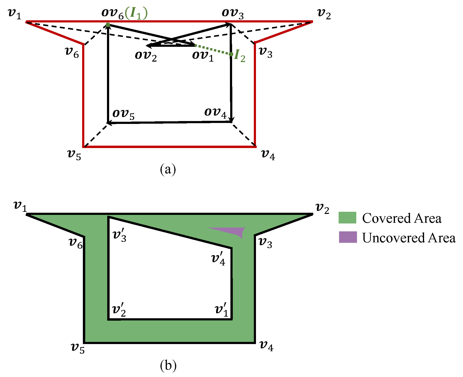
Lee et al. [26] classified the possible distributions of $inv\_dir$ and $inv\_pos$ into five categories: CASE 1.1, CASE 1.2, CASE 2, CASE 3.1, and CASE 3.2; however, through extensive exploration, we found that the existing cases do not encompass all possible situations. For instance, CASE 3.2 was designed to address scenarios where more than two directionally invalid offset edges occur during the offset process, but it only handles cases where the backward edge and forward edge are parallel. In practice, the backward and forward edges are often not parallel. Even when the backward and forward edges are parallel, the method used in CASE 3.2 can still result in incomplete coverage. As shown in Figure 3a, the vertices of the previous shrinking ring are labeled as ${\mathit{v}}_1$ to ${\mathit{v}}_6$. Among these, the edges $\left({\mathit{v}}_5{\mathit{v}}_6\right)$ and $\left({\mathit{v}}_3{\mathit{v}}_4\right)$ are parallel. The offset vertices corresponding to these are labeled as ${\mathit{ov}}_1$ to ${\mathit{ov}}_6$. When $\left({\mathit{ov}}_5{\mathit{ov}}_6\right)$ is the backward edge and $\left({\mathit{ov}}_3{\mathit{ov}}_4\right)$ is the forward edge, ${\mathit{I}}_1$ and ${\mathit{I}}_2$ are the intersection points chosen by the CASE 3.2 strategy. In Figure 3b, the current shrinking ring consists of vertices ${\mathit{v}}_1^{\prime }$ to ${\mathit{v}}_4^{\prime }$. By flying along these two shrinking rings, the UAV is unable to fully cover the intermediate area.

Based on these observations, we have reorganized the cases into CASE 1, CASE 2, CASE 3.1, CASE 3.2, and CASE 3.3, improving the algorithm to address all scenarios during the offset process.

CASE 1: $inv\_dir=0$ and $inv\_pos=0$. There are no invalid offset edges in terms of direction or position between the backward edge and the forward edge. For this case, it is sufficient to include the terminal offset vertex of the backward edge in $\mathit{EVL}$. As illustrated in Figure 4a, $\left({\mathit{ov}}_1{\mathit{ov}}_2\right)$ represents the backward edge and $\left({\mathit{ov}}_2{\mathit{ov}}_3\right)$ represents the forward edge; therefore, only ${\mathit{ov}}_2$ should be added to $\mathit{EVL}$.

CASE 2: $inv\_dir=0$ and $inv\_pos\ge 1$. All offset edges between the backward edge and the forward edge are valid in terms of direction, but there is at least one positionally invalid offset edge. In this case, these offset edges result in globally invalid loops. We begin by sequentially adding the terminal offset vertex of the backward edge, all intermediate offset vertices, and the initial offset vertex of the forward edge to the $\mathit{EVL}$. Trimming is performed subsequently. As depicted in Figure 4b, $\left({\mathit{ov}}_2{\mathit{ov}}_3\right)$ represents the backward edge and $\left({\mathit{ov}}_4{\mathit{ov}}_5\right)$ represents the forward edge; thus, ${\mathit{ov}}_3$ and ${\mathit{ov}}_4$ are added to $\mathit{EVL}$ in sequence. Figure 4c shows the globally invalid loop generated by $\left({\mathit{ov}}_2{\mathit{ov}}_3\right)$, $\left({\mathit{ov}}_3{\mathit{ov}}_4\right)$, $\left({\mathit{ov}}_4{\mathit{ov}}_5\right)$, and $\left({\mathit{ov}}_7{\mathit{ov}}_8\right)$.

CASE 3.1: $inv\_dir=1$. There is only one directionally invalid offset edge between the backward edge and the forward edge. The strategy for handling this case is to determine the intersection point between the backward edge and the forward edge and add it to $\mathit{EVL}$. As shown in the Figure 4d, $\left({\mathit{ov}}_1{\mathit{ov}}_2\right)$ represents the backward edge and $\left({\mathit{ov}}_3{\mathit{ov}}_4\right)$ represents the forward edge. Because $\left({\mathit{ov}}_2{\mathit{ov}}_3\right)$ is a directionally invalid edge, the intersection point $\mathit{I}$ between $\left({\mathit{ov}}_1{\mathit{ov}}_2\right)$ and $\left({\mathit{ov}}_3{\mathit{ov}}_4\right)$ is added to $\mathit{EVL}$.

CASE 3.2: $inv\_dir\ge 2$ and the backward edge intersects the forward edge. The approach for this scenario is the same as in CASE 3.1. Figure 4e illustrates that $\left({\mathit{ov}}_4{\mathit{ov}}_5\right)$ is the backward edge and $\left({\mathit{ov}}_7{\mathit{ov}}_1\right)$ is the forward edge. The edges $\left({\mathit{ov}}_5{\mathit{ov}}_6\right)$ and $\left({\mathit{ov}}_6{\mathit{ov}}_7\right)$ situated between them are directionally invalid. We calculate the intersection point $\mathit{I}$ of $\left({\mathit{ov}}_4{\mathit{ov}}_5\right)$ and $\left({\mathit{ov}}_7{\mathit{ov}}_1\right)$ and add it to $\mathit{EVL}$.

CASE 3.3: $inv\_dir\ge 2$ and the backward edge does not intersect the forward edge. The method here involves first sequentially traversing the directionally invalid offset edges between the backward and forward edges, then calculating their intersection point $\{{\mathit{I}}_1^1,{\mathit{I}}_1^2,...,{\mathit{I}}_1^i,...{\mathit{I}}_1^{inv\_dir}\}$ with the backward edge. Subsequently, the minimum distance $d_{{\mathit{I}}_1^i}$ between ${\mathit{I}}_1^i$ and all original edges is calculated. Then, ${\mathit{I}}_1^i$ is added to the preselected list only if it lies inside the shrinking ring and $d_{{\mathit{I}}_1^i}\ge L_1-L_1^{\prime }$. The shortest distance from the points in the preselected list to the original edges is expressed as $d^{*}=\min \left\{d_{{\mathit{I}}_1^i}\right|d_{{\mathit{I}}_1^i}\ge L_1-L_1^{\prime }\}$. Finally, the ${\mathit{I}}_1^i$ corresponding to $d^{*}$ from the preselected list is selected and added to $\mathit{EVL}$. The intersection point ${\mathit{I}}_2$ with the forward edge is then added to $\mathit{EVL}$ using the same procedure. As shown in Figure 4f, $\left({\mathit{ov}}_5{\mathit{ov}}_6\right)$ represents the backward edge and $\left({\mathit{ov}}_3{\mathit{ov}}_4\right)$ represents the forward edge. The intersection points of $\left({\mathit{ov}}_6{\mathit{ov}}_1\right)$, $\left({\mathit{ov}}_1{\mathit{ov}}_2\right)$, and $\left({\mathit{ov}}_2{\mathit{ov}}_3\right)$ with $\left({\mathit{ov}}_5{\mathit{ov}}_6\right)$ are ${\mathit{I}}_1^1$,${\mathit{I}}_1^2$,${\mathit{I}}_1^3$, respectively. Given that $d_{{\mathit{I}}_1^1}<L_1-L_1^{\prime }$ and $d_{{\mathit{I}}_1^2}<d_{{\mathit{I}}_1^3}$, ${\mathit{I}}_1^2$ is set as ${\mathit{I}}_1$ and added to $\mathit{EVL}$. Similarly, ${\mathit{I}}_2$ from the intersection points with $\left({\mathit{ov}}_3{\mathit{ov}}_4\right)$ is added to $\mathit{EVL}$.

According to CASE 2, $\mathit{EVL}$ may form globally invalid loops. These loops fall entirely within the UAV’s photography range as it follows the previous shrinking ring. This results in no improvement in coverage and increases the path length. To eliminate these globally invalid loops, we identify the self-intersection points within the overall loop formed by $\mathit{EVL}$. Based on these points, we trim the line segments and ultimately extract the shrinking rings.

To facilitate a clearer understanding of the process of generating shrinking rings, the full pseudocode of the algorithm is provided in Algorithm 1.

Algorithm 1 Generate the Shrinking Ring List for the Region

Input: Region ${\mathit{R}}_m=({\mathit{v}}_m^1,{\mathit{v}}_m^2,...,{\mathit{v}}_m^{r_m})$, the longitudinal scanning length $L_1$, the overlap length in the longitudinal direction $L_1^{\prime }$ Output: The shrinking ring list ${\mathit{SRL}}_m$ = $({\mathit{S}}_m^1,{\mathit{S}}_m^2,...,{\mathit{S}}_m^{idx},...,{\mathit{S}}_m^{n_m})$, where $n_m$ denotes the number of shrinking rings, varying by region.  1: ${\mathit{SRL}}_m\leftarrow \left(\right)$  2: Initialize the list ${\mathit{T}}_1$ to store the shrinking rings to be offset: ${\mathit{T}}_1\leftarrow \left({\mathit{R}}_m\right)$  3: while${\mathit{T}}_1\ne \left(\right)$do  4:     Set the previous shrinking ring: $\mathit{S}\leftarrow$ the head of ${\mathit{T}}_1$  5:     Append $\mathit{S}$ to the tail of ${\mathit{SRL}}_m$  6:     Generate $\mathit{OVL}$ from $\mathit{S}$  7:     Generate $\mathit{OEL}$ from $\mathit{OVL}$  8:     Set the $off\_pos$ and $off\_div$ attributes for each offset edge in $\mathit{OEL}$  9:     Iterate through $\mathit{OEL}$ and extract $\mathit{EVL}$ based on different cases. 10:     Connect adjacent vertices in $\mathit{EVL}$ to form extracted edge list $\mathit{EEL}$. 11:     Insert intersection points into the $\mathit{EVL}$ based on the intersections of the edges in the $\mathit{EEL}$. 12:     Reconstruct $\mathit{EEL}$ based on the new $\mathit{EVL}$. 13:     Remove edges from the $\mathit{EEL}$ that are within a minimum distance of less than $L_1-L_1^{\prime }$ from each edge of $\mathit{S}$ 14:     Initialize the list ${\mathit{T}}_2$ to store the offset edges: ${\mathit{T}}_2\leftarrow \left(\right)$ 15:     for $i\leftarrow 1$ to size of $\mathit{EEL}$ do 16:         Append $\mathit{EEL}\left[i\right]$ to the tail of ${\mathit{T}}_2$ 17:         $end\leftarrow$ size of ${\mathit{T}}_2$ 18:         $begin\leftarrow end-1$ 19:         while $begin\ge 1$ do 20:             if the start vertex of ${\mathit{T}}_2\left[begin\right]$ = the end vertex of ${\mathit{T}}_2\left[end\right]$ then 21:                  Form ${\mathit{S}}_m^{idx}$ by extracting the start vertices of edges indexed from $begin$ to $end$ 22:                  Append ${\mathit{S}}_m^{idx}$ to the head of ${\mathit{T}}_1$ 23:                  Remove edges in ${\mathit{T}}_2$ with indices from $begin$ to $end$ 24:                  $\mathbf{break}$ 25:             else 26:                  $begin\leftarrow begin-1$ 27:             end if 28:         end while 29:     end for 30: end while

3.2. Waypoint Generation

After the shrinking ring has been generated, waypoints must be created along each segment to ensure subsequent coverage by multiple UAVs. For a segment of length l in a shrinking ring, the number of waypoints $l_n$ is calculated as follows:

$$l_n=⌈{\displaystyle \frac{l-\frac{L_2}{2}}{l_g}}⌉$$

(8)

where $l_g=L_2-L_2^{\prime }$ denotes the distance between waypoints. To ensure that waypoints are evenly spaced, $L_2^{\prime }$ should be adjusted according to the value of $l_n$. This adjustment is expressed as follows:

$$\overline{L_2^{\prime }}={\displaystyle \frac{\left(l_n-\frac{1}{2}\right)L_2-l}{l_n-1}}.$$

(9)

Accordingly, the interval distance $l_g$ between waypoints should be revised to $\overline{l_g}$. This revised interval is expressed as

$$\overline{l_g}=L_2-\overline{L_2^{\prime }}.$$

(10)

3.3. Connecting Waypoints

To obtain the optimal coverage path, the first step is to determine the regional access order. A widely-used strategy involves treating the center of each region as a representative point and optimizing the visit sequence of these centers using a TSP solver [17,18,19,20,27]. Therefore, we utilize the Self-Organizing Map (SOM) [28] algorithm to establish the visiting order of regions, which is a well-documented method used in previous studies [29,30]. After the visit order of the regions is determined, the corresponding ${\mathit{SRL}}_m$ is arranged accordingly. Then, the optimal coverage path can be formed by sequentially connecting the waypoints in each shrinking ring ${\mathit{S}}_m^{idx}$ of ${\mathit{SRL}}_m$.

For ${\mathit{S}}_m^{idx}=({\mathit{w}}_{m,idx}^1,{\mathit{w}}_{m,idx}^2,...,{\mathit{w}}_{m,idx}^{n_{idx}})$, $n_{idx}$ represents the number of waypoints in the shrinking ring, while ${\mathit{w}}_{m,idx}^{n_{idx}}$ denotes the $n_{idx}$-th waypoint of the $idx$-th shrinking ring generated by region $R_m$. Thus, there are $n_{idx}$ possible ways to integrate ${\mathit{S}}_m^{idx}$ into the optimal coverage path: ${\mathit{P}}_{m,idx}=\{({\mathit{w}}_{m,idx}^1,{\mathit{w}}_{m,idx}^2,...,{\mathit{w}}_{m,idx}^{n_{idx}}),({\mathit{w}}_{m,idx}^2,{\mathit{w}}_{m,idx}^3,...,{\mathit{w}}_{m,idx}^1),...,({\mathit{w}}_{m,idx}^{n_{idx}},{\mathit{w}}_{m,idx}^1,...,{\mathit{w}}_{m,idx}^{n_{idx}-1})\}$. Suppose that in the $n_{idx}$-th sub-path of ${\mathit{P}}_{m,idx}$, the first waypoint is denoted as ${\mathit{P}}_{m,idx}^{n_{idx},1}$ and the last waypoint is denoted as ${\mathit{P}}_{m,idx}^{n_{idx},n_{idx}}$. Then, the cost of ${\mathit{P}}_{m,idx}^{n_{idx}}$ is computed based on the waypoint ${\mathit{P}}_{m,idx}^{n_{idx},1}$ and ${\mathit{P}}_{m,idx}^{n_{idx},n_{idx}}$ using the following formula:

$$\begin{array}{cc}\hfill {\mathit{P}}_{m,idx}^{n_{idx}}=& {\lambda }_1\times (\mathrm{d}({\mathit{P}}_{m,idx}^{n_{idx},1},{\mathit{w}}_b)-\mathrm{d}({\mathit{P}}_{m,idx}^{n_{idx},1},{\mathit{P}}_{m,idx}^{n_{idx},n_{idx}}))\hfill \\ & +{\lambda }_2\times (\mathrm{a}({\mathit{w}}_b,{\mathit{P}}_{m,idx}^{n_{idx},1},{\mathit{P}}_{m,idx}^{n_{idx},2})-\mathrm{a}({\mathit{P}}_{m,idx}^{n_{idx},n_{idx}},{\mathit{P}}_{m,idx}^{n_{idx},1},{\mathit{P}}_{m,idx}^{n_{idx},2}))\hfill \end{array}$$

(11)

where ${\mathit{w}}_b$ refers to the backward reference point, typically the last waypoint of the previous-level shrinking ring. However, for the first-level shrinking ring, ${\mathit{w}}_b$ corresponds to the warehouse. This indicates that when forming the optimal coverage path, the connection between ${\mathit{P}}_{m,idx}^{n_{idx},1}$ and ${\mathit{P}}_{m,idx}^{n_{idx},n_{idx}}$ in the current shrinking ring ${\mathit{S}}_m^{idx}$ is broken and ${\mathit{P}}_{m,idx}^{n_{idx},1}$ is connected to ${\mathit{w}}_b$, resulting in new distance and turning costs. Thus, the connection way is determined as follows:

$${\mathit{P}}_{m,idx}^{*}=\underset{m\in [1,M]}{\mathrm{argmin}}{\mathit{P}}_{m,idx}^{n_{idx}}.$$

(12)

Based on this, the pseudocode for the first stage of SSDP is presented in Algorithm 2.

Algorithm 2 Generate the Optimal Coverage Path

Input: Region set $\left\{{\mathit{R}}_m\right\}$, the longitudinal and lateral scanning length $L_1,L_2$, the overlap length in the longitudinal and lateral direction $L_1^{\prime },L_2^{\prime }$, warehouse ${\mathit{w}}_0$, the weights for distance and turning in energy consumption ${\lambda }_1$ and ${\lambda }_2$ Output: A optimal coverage path $\mathit{G}=({\mathit{w}}_1,{\mathit{w}}_2,\dots ,{\mathit{w}}_g,\dots ,{\mathit{w}}_G)$  1: for $m\leftarrow 1$ to M do  2:    Generate ${\mathit{SRL}}_m=({\mathit{S}}_m^1,{\mathit{S}}_m^2,...,{\mathit{S}}_m^{n_m})$ by ${\mathit{R}}_m$ using Algorithm 1  3:    for ${\mathit{S}}_m^{idx}\in {\mathit{SRL}}_m$ do  4:       Traverse each edge of ${\mathit{S}}_m^{idx}$ and insert waypoints  5:    end for  6: end for  7: Determine the region visitation order using a TSP solver (SOM)  8: $\mathit{G}\leftarrow \left(\right)$  9: for $m\leftarrow 1$ to M do 10:    Retrieve the ${\mathit{SRL}}_m$ corresponding to the m-th region in the visitation order 11:    for ${\mathit{S}}_m^{idx}\in {\mathit{SRL}}_m$ do 12:       Merge ${\mathit{S}}_m^{idx}$ into the tail of $\mathit{G}$ according to ${\mathit{P}}_{m,idx}^{*}$, calculated by Equation (12) 13:    end for 14: end for

4. Path Segmentation

Given that the optimal coverage path $\mathit{G}=({\mathit{w}}_1,{\mathit{w}}_2,\dots ,{\mathit{w}}_g,\dots ,{\mathit{w}}_G)$ is formed by sequenced waypoints, multiple UAVs can achieve collaborative coverage by having each take on non-overlapping segments of the path. When using waypoints as the units of segmentation, the minimum energy consumption problem for the UAV swarm transforms into a combinatorial optimization problem. Specifically, we regard each waypoint as a decision stage; during the solution process, each stage must be considered sequentially, with each stage having its own optimal solution. Additionally, to determine the optimal solution for a stage, we must consider the optimal solutions of all preceding stages. Put another way, this problem is characterized by optimal substructure and overlapping subproblems, making the DP-based method the appropriate solution.

4.1. State Transition Matrix Design

The state transition matrix crucial for correctly solving problems and finding the optimal solution with the DP algorithm. Here, we design a two-dimensional matrix $\mathit{D}$ as the state transition matrix. The length of $\mathit{D}$ corresponds to the number of waypoints in $\mathit{G}$ and its width is determined by the maximum number of available drones N. The value $\mathit{D}\left[n\right]\left[g\right]$ in the matrix represents the subproblem, that is, the minimum energy consumption for visiting the first g waypoints with n drones.

4.2. Initialization and State Transition

Before initialization, the distances and angles between waypoints are precomputed and stored in the arrays $\mathit{l}$ and $\mathit{a}$. These precomputations are defined as follows:

$$\mathit{l}\left[g\right]=\left\{\begin{array}{cc}0,\hfill & g=1\hfill \\ \mathit{l}[g-1]+\mathrm{d}({\mathit{w}}_{g-1},{\mathit{w}}_g),\hfill & 1<g\le G\hfill \end{array}\right.$$

(13)

$$\mathit{a}\left[g\right]=\left\{\begin{array}{cc}0,\hfill & g=1\hfill \\ \mathit{a}[g-1]+\mathrm{a}({\mathit{w}}_{g-1},{\mathit{w}}_g,{\mathit{w}}_{g+1}),\hfill & 1<g<G\hfill \end{array}\right.$$

(14)

where $\mathit{l}\left[g\right]$ represents the total path distance from waypoint ${\mathit{w}}_1$ to waypoint ${\mathit{w}}_g$ in the optimal coverage path and $\mathit{a}\left[g\right]$ represents the total path angle from waypoint ${\mathit{w}}_1$ to waypoint ${\mathit{w}}_{g+1}$. Here, $\mathrm{d}(·,·)$ denotes the Euclidean distance between two waypoints and $\mathrm{a}(·,·,·)$ represents the turning angle of the path formed by three sequential waypoints.

We initialize each element in the first row of $\mathit{D}$ using the following formula.

$$\mathit{D}\left[1\right]\left[g\right]=\left\{\begin{array}{ll}{\lambda }_1\times 2\times \mathrm{d}({\mathit{w}}_0,{\mathit{w}}_1)+{\lambda }_2\times \mathrm{a}({\mathit{w}}_0,{\mathit{w}}_1,{\mathit{w}}_0),& g=1\hfill \\ \begin{array}{c}{\lambda }_1\times \left(\mathrm{d}({\mathit{w}}_0,{\mathit{w}}_1)+\mathit{l}\left[g\right]+\mathrm{d}({\mathit{w}}_g,{\mathit{w}}_0)\right)\hfill \\ +{\lambda }_2\times \left(\mathrm{a}({\mathit{w}}_0,{\mathit{w}}_1,{\mathit{w}}_2)+\mathit{a}[g-1]+\mathrm{a}({\mathit{w}}_{g-1},{\mathit{w}}_g,{\mathit{w}}_0)\right),\hfill \end{array}\hfill & 1<g\le G\hfill \end{array}\right.$$

(15)

This indicates that the first drone starts from depot ${\mathit{w}}_0$, visits ${\mathit{w}}_1,{\mathit{w}}_2,...,{\mathit{w}}_G$ in sequence, and then returns to the depot. After this calculation, the values must be checked to eliminate infeasible scenarios, as expressed below:

$$\mathit{D}\left[1\right]\left[g\right]=\left\{\begin{array}{cc}\mathit{D}\left[1\right]\left[g\right],\hfill & \mathit{D}\left[1\right]\left[g\right]\le E\hfill \\ +\infty ,\hfill & \mathit{D}\left[1\right]\left[g\right]>E\hfill \end{array}\right.$$

(16)

where $\mathit{D}\left[1\right]\left[g\right]$ represents the energy cost for UAV $u_1$ to travel sequentially from the warehouse ${\mathit{w}}_0$ through intermediate waypoints ${\mathit{w}}_1,{\mathit{w}}_2,...$, finally reaching ${\mathit{w}}_g$ before returning to the warehouse. If this energy cost exceeds its energy constraint, the process is deemed infeasible and the cost is set to infinity. At this point, the reachable waypoints are temporarily assigned to $u_1$, while the unreachable waypoints are assigned to other UAVs for completion.

Then, the first column of $\mathit{D}$ is initialized as follows:

$$\mathit{D}\left[n\right]\left[1\right]={\lambda }_1\times 2\times \mathrm{d}({\mathit{w}}_0,{\mathit{w}}_1)+{\lambda }_2\times \mathrm{a}({\mathit{w}}_0,{\mathit{w}}_1,{\mathit{w}}_0),1\le n\le N.$$

(17)

This shows that when there is only one waypoint ${\mathit{w}}_1$ in the path; the drone departs from the warehouse ${\mathit{w}}_0$, visits ${\mathit{w}}_1$, and immediately returns to ${\mathit{w}}_0$. Furthermore, because $\mathit{D}\left[1\right]\left[1\right]=\mathit{D}\left[2\right]\left[1\right]=...=\mathit{D}\left[N\right]\left[1\right]$, only the first drone is required for this task, while the other drones can remain on standby.

Continuing with the matrix solution, we focus on the remaining components; $\mathit{D}\left[n\right]\left[g\right]$ can be derived from the subproblem $\mathit{D}[n-1]\left[k\right]$, with its value calculated as follows:

$$t_k=\mathit{D}[n-1]\left[k\right]+{\lambda }_1\times t_k^1+{\lambda }_2\times t_k^2,$$

(18)

$$1\le k<g,2\le g\le G,2\le n\le N$$

where $t_k$ is a candidate for $\mathit{D}\left[n\right]\left[g\right]$ composed of $\mathit{D}[n-1]\left[k\right]$, $t_k^1$, $t_k^2$. Specifically, $t_k^1$ represents the distance cost for the n-th UAV, expressed as

$$t_k^1=\mathrm{d}({\mathit{w}}_0,{\mathit{w}}_{k+1})+\mathit{l}\left[g\right]-\mathit{l}[k+1]+\mathrm{d}({\mathit{w}}_g,{\mathit{w}}_0),1\le k<g.$$

(19)

Meanwhile, $t_k^2$ denotes the turning cost for the n-th UAV, described as follows.

$$t_k^2=\left\{\begin{array}{cc}\begin{array}{c}\mathrm{a}({\mathit{w}}_0,{\mathit{w}}_{k+1},{\mathit{w}}_{k+2})+\mathit{a}[g-1]\hfill \\ -\mathit{a}[k+1]+\mathrm{a}({\mathit{w}}_{g-1},{\mathit{w}}_g,{\mathit{w}}_0),\hfill \end{array}\hfill & 1\le k<g-1\hfill \\ \mathrm{a}({\mathit{w}}_0,{\mathit{w}}_g,{\mathit{w}}_0),\hfill & k=g-1\hfill \end{array}\right.$$

(20)

This formulation assumes that the first k waypoints are handled by the first $n-1$ UAVs. The n-th UAV begins its route at the warehouse, sequentially visits waypoints ${\mathit{w}}_{k+1},{\mathit{w}}_{k+2},...,{\mathit{w}}_g$, and returns to the warehouse. The value of $\mathit{D}\left[n\right]\left[g\right]$ is then determined as the smallest $t_k$ among all candidates.

Therefore, the optimal solution for $\mathit{DP}\left[n\right]\left[g\right]$ can be obtained from these values as follows:

$$\mathit{D}\left[n\right]\left[g\right]=\underset{1\le k<g}{min}\{t_k\mid t_k-\mathit{D}[n-1]\left[k\right]\le E\}.$$

(21)

Alternatively, if the value of $\mathit{D}\left[n\right]\left[g\right]$ calculated from the above formula is greater than $\mathit{D}[n-1]\left[g\right]$, then $\mathit{D}\left[n\right]\left[g\right]$ should be set to $\mathit{D}[n-1]\left[g\right]$. This indicates that all g waypoints are to be handled by the first $n-1$ UAVs, meaning that the n-th UAV is not needed, that is, the optimal solution can be achieved with only the first $n-1$ UAVs. The final expression for $\mathit{D}\left[n\right]\left[g\right]$ is as follows:

$$\mathit{D}\left[n\right]\left[g\right]=min\left(\mathit{D}[n-1]\left[g\right],\underset{1\le k<g}{min}\{t_k\mid t_k-\mathit{D}[n-1]\left[k\right]\le E\}\right).$$

(22)

Finally, the values in the last row and last column of the matrix signify the minimum energy consumption for the UAV swarm. The time complexity of the path segment algorithm is primarily determined by this part. The time complexity is $O\left(N{G}^2\right)$, where N represents the number of drones and G denotes the number of waypoints in the optimal coverage path. In practice, the computation can stop when $\mathit{D}\left[n\right]\left[G\right]$ equals $\mathit{D}[n-1]\left[G\right]$, which indicates that the n-th drone and all subsequent drones are not required for coverage.

4.3. Tracing the Optimal Solution

After the optimal solution is determined, we can trace back through the state transition matrix to allocate waypoints to each UAV. We start from the last element in the final row, $\mathit{D}\left[N\right]\left[G\right]$; if $\mathit{D}\left[N\right]\left[G\right]=\mathit{D}[N-1]\left[G\right]$, it implies that the N-th UAV was not employed and no waypoints were assigned to it. Otherwise, we should trace back using Equation (21) to determine that it was derived from $\mathit{D}[N-1]\left[k\right]$ and assign the waypoints $({\mathit{w}}_{k+1},...,{\mathit{w}}_G)$ to the N-th drone. Next, we determine the waypoints assigned to the $(N-1)$-th drone in the same manner from $\mathit{D}[N-1]\left[k\right]$. Finally, when $n=1$, all remaining waypoints are allocated to the first UAV. The steps of the algorithm are presented in Algorithm 3.

Algorithm 3 Path Segmentation

Input: the optimal coverage path $\mathit{G}=({\mathit{w}}_1,{\mathit{w}}_2,\dots ,{\mathit{w}}_g,\dots ,{\mathit{w}}_G)$, warehouse ${\mathit{w}}_0$, the weights for distance and turning in energy consumption ${\lambda }_1$ and ${\lambda }_2$, energy constraint E Output: the flight paths for UAVs $\{{\mathit{W}}_1,{\mathit{W}}_2,...,{\mathit{W}}_n\}$  1: for $g\leftarrow 1$ to G do  2:     Calculate the elements of array $\mathit{l}$ and $\mathit{a}$ by Equations (13) and (14), respectively.  3: end for  4: Initialize the first row of $\mathit{D}$ by Equation (15).  5: Check whether the first row of $\mathit{D}$ satisfies the energy constraints using Equation (16).  6: Initialize the first column of $\mathit{D}$ by Equation (17).  7: for $n\leftarrow 2$ to N do  8:     for $g\leftarrow 2$ to G do  9:          Calculate the value of $\mathit{D}\left[n\right]\left[g\right]$ by Equation (22). 10:    end for 11: end for 12: $g\leftarrow G$ 13: for $n\leftarrow N$ to 1 do 14:     if $n=1$ then 15:         Assign the waypoint sequence ${\mathit{W}}_1=({\mathit{w}}_0,{\mathit{w}}_1,\cdots ,{\mathit{w}}_g,{\mathit{w}}_0)$ to UAV $u_1$. 16:         break 17:     end if 18:     if $\mathit{D}\left[n\right]\left[g\right]=\mathit{D}[n-1]\left[g\right]$ then 19:         Assign the waypoint sequence ${\mathit{W}}_n=\left(\right)$ to UAV $u_n$. 20:     else 21:         for $k\leftarrow 1$ to $g-1$ do 22:             if $\mathit{D}\left[n\right]\left[g\right]$ is derived from $\mathit{D}[n-1]\left[k\right]$ by Equation (21) then 23:                Assign the waypoint sequence ${\mathit{W}}_n=({\mathit{w}}_0,{\mathit{w}}_{k+1},\cdots ,{\mathit{w}}_g,{\mathit{w}}_0)$ to UAV $u_n$. 24:                $g\leftarrow k$ 25:             end if 26:         end for 27:     end if 28: end for

5. Experiments and Discussion

In this section, we describe some simulation scenarios created for our computational experiments. Visual Studio Code 1.87.0 was the simulation experiment platform software, and the hardware setup of the experimental system included a 2.4 GHz 4-Core Intel Core i5 processor, with the programming language being C++. The analysis of tables and line charts was conducted using OriginPro 2021. The path simulation diagrams were created using the matplotlib library in Python.

5.1. Parameter Setting

For the experiments, the field of view for the UAV cameras was configured to 4 m × 4 m. The images captured by the drones were required to have an overlap of 1 m in both length and width. The maximum energy consumption for each UAV was capped at 1000 kJ. Each drone was required to depart from the warehouse, complete the coverage task, and return to the warehouse.

The specific parameter settings of the map along with the target regions are shown in

Table 1. Parameter settings of the map and target regions.

Parameter	Value
Map coordinate (m, m)	((0, 0), (0, 400), (400, 400), (400, 0))
Warehouse coordinate (m, m)	(200, 200)
Region shape
Number of regions	Refer to specific experiments
Locations of regions	Randomly distributed in the map
Angles of regions	${\displaystyle \frac{\pi }{\mathrm{Number}\mathrm{of}\mathrm{regions}}}\times$ index

. These regions are either convex or non-convex. In order to exclude the influence of the shape of the region, all convex regions had the same shape and all non-convex regions had the same shape. Each region was equal in size; in addition, the warehouse coordinate was not located within any region, and all regions did not intersect with each other.

In order to verify the effectiveness and superiority of SSDP, we set up the following three experimental scenarios and used the total energy consumption of the UAV swarm as the experimental evaluation metric:

• Increasing the proportion of non-convex regions in the total regions; the experimental details are provided in Section 5.2.
• Increasing the total area while maintaining the ratio of convex to non-convex regions; the experimental details are provided in Section 5.3.
• Increasing the number of UAVs; the experimental details are provided in Section 5.4.
• Adjusting the decomposition strategy; the experimental details are provided in Section 5.5.

The following models were selected as comparison models:

• Benchmark model: B&F-Avg. In this model, the SOM method is used to determine the visitation order of regions, after which the B&F pattern coverage paths are generated for each region according to the visitation order. These paths are then connected end-to-end to form a optimal coverage path. Finally, the optimal coverage path is segment equally among the UAVs based on length.
• Ablation model: B&F-DP. The only difference between this method and B&F-Avg is the use of the DP-based method to segment the optimal coverage path among the UAVs.
• State-of-the-art methods: GASC [20] and BINPAT [23].

Because the B&F pattern cannot be applied directly to non-convex regions, these methods require pre-decomposing the regions into convex parts.

5.2. Increasing the Proportion of Non-Convex Regions

In this experiment, a total of 20 convex regions were randomly generated. These regions were gradually replaced by non-convex regions in increments of 2. The number of UAVs was set at 3.

Table 2. The UAV swarm’s total path distance (m) for each model with different proportions of non-convex regions.

Proportion	B&F-Avg	B&F-DP	SSDP	BINPAT	GASC
0	9453.91	8852.40	8877.79	9875.32	8662.26
10	9635.92	9113.07	8915.15	9768.66	8765.68
20	9926.45	9329.50	8977.68	9976.71	8882.51
30	10,139.30	9695.32	9010.03	10,097.40	9005.72
40	10,458.70	9799.72	9035.02	10,322.20	9253.09
50	10,728.44	10,104.42	9059.61	10,432.50	9388.63
60	10,807.22	10,427.86	9076.22	10,445.20	9572.77
70	11,145.19	10,583.82	9102.90	9979.21	9751.16
80	11,362.74	10,850.81	9149.90	10,100.30	9802.40
90	11,569.86	11,096.35	9172.03	10,261.30	9912.20
100	11,921.05	11,343.37	9208.48	10,339.50	10,150.06

,

Table 3. The UAV swarm’s total path angle (°) for each model with different proportions of non-convex regions.

Proportion	B&F-Avg	B&F-DP	SSDP	BINPAT	GASC
0	27,511.61	27,202.47	41,881.81	31,130.10	26,961.34
10	28,603.41	28,242.96	42,004.70	32,988.10	29,468.20
20	29,497.60	29,150.81	41,615.97	35,089.50	32,155.66
30	30,130.43	30,313.16	41,798.76	35,965.50	34,801.66
40	31,200.70	31,031.21	41,616.96	38,758.70	37,027.66
50	32,888.65	32,068.54	41,535.77	42,083.30	39,871.62
60	33,684.15	33,343.08	41,398.59	42,127.00	42,634.80
70	34,446.90	34,050.46	41,173.71	42,015.30	45,167.94
80	35,363.35	35,101.21	40,996.62	44,351.90	48,558.80
90	36,326.30	36,109.54	41,051.14	45,502.80	50,310.08
100	37,637.10	36,977.18	40,844.73	47,887.80	53,941.52

and

Table 4. The UAV swarm’s total energy consumption (kJ) for each model with different proportions of non-convex regions.

Proportion	B&F-Avg	B&F-DP	SSDP	BINPAT	GASC
0	1299.58	1231.88	1387.26	1382.38	1208.99
10	1330.44	1270.64	1392.55	1390.27	1246.15
20	1370.89	1303.29	1395.21	1434.43	1286.62
30	1400.28	1354.59	1400.58	1456.48	1327.35
40	1445.65	1373.25	1401.37	1509.63	1377.01
50	1492.13	1416.70	1403.16	1556.03	1421.12
60	1508.84	1464.63	1403.51	1557.84	1469.60
70	1553.01	1488.71	1404.03	1506.73	1515.07
80	1585.86	1528.25	1407.23	1544.01	1555.82
90	1618.08	1565.06	1410.17	1573.24	1585.81
100	1669.36	1600.57	1411.93	1606.42	1649.07

list the statistical results for the UAV swarm’s total path distance, total path angle, and energy consumption, respectively. Figure 5 illustrates the changes in energy consumption as the proportion of non-convex regions increases. Figure 6 shows the UAV swarm paths generated by each model when all regions are non-convex.

From Table 2 and Table 3 and Figure 5, it can be observed that the path generated by GASC is consistently the shortest among those produced by methods based on the B&F pattern, which include B&F-Avg, B&F-DP, and BINPAT. This holds true across different proportions of non-convex regions. However, when the proportion exceeds 10%, the total turning angle of GASC becomes greater than that of B&F-Avg and B&F-DP. When the proportion exceeds 60%, it also surpasses BINPAT. Consequently, when the proportion exceeds 70%, the energy consumption of GASC surpasses that of B&F-DP and BINPAT. This indicates that the shortest path does not necessarily result in the lowest energy consumption. Additionally, because the B&F pattern requires decomposing concave regions for coverage, the path length of GASC exceeds that of SSDP when the proportion of non-convex regions surpasses 40%.

Unlike other methods, BINPAT uses the nearest-neighbor approach to determine the order of region visits. This approach is highly influenced by the shape and location of the regions, meaning that its energy consumption does not always increase with the proportion of non-convex regions. However, it still shows an overall upward trend. As the proportion of non-convex regions increases, the number of subregions generated by decomposition also rises, narrowing the gap between the nearest-neighbor method and the TSP solver. Consequently, when the proportion exceeds 70%, BINPAT’s energy consumption is lower than that of B&F-Avg and GASC, although it still falls short compared to B&F-DP and SSDP. This suggests that in order to achieve the lowest energy consumption, a TSP solver should be used to determine the order of region visits.

The energy consumption of SSDP falls below that of BINPAT when the proportion of non-convex regions reaches 20%, below B&F-Avg at 40%, and subsequently falls below B&F-DP and GASC at 50%. This demonstrates the superiority of optimal coverage path generation in handling non-convex regions. B&F-DP consistently consumes less energy than B&F-Avg and BINPAT, and its energy consumption drops below that of GASC when the proportion of non-convex regions exceeds 40%, proving the effectiveness of the DP-based approach. Additionally, as shown in Figure 6, SSDP and B&F-DP require only two UAVs to complete the coverage task in all scenarios. This indicates that the DP-based approach not only reduces the total energy consumption of the UAV swarm but also conserves UAV resources.

5.3. Increasing the Total Area

In this section, the ratio of convex to non-convex regions was set to 1:1, then the number of regions was increased from 4 to 28 in increments of 4. The number of UAVs was 3.

Table 5. The UAV swarm’s total path distance (m) for each model as the number of regions increases.

Region Number	B&F-Avg	B&F-DP	SSDP	BINPAT	GASC
4	3148.27	2556.98	2347.72	2968.14	2515.72
8	5207.67	4530.11	4132.77	4918.77	4307.10
12	7276.99	6542.73	6005.10	6969.96	6208.62
16	8881.28	8345.74	7511.54	7977.63	7754.37
20	10,619.30	10,131.65	9037.13	9788.74	9562.48
24	12,397.00	11,905.30	10,583.57	11,641.30	11,091.75
28	14,413.50	13,825.00	12,268.36	13,245.60	12,971.58

,

Table 6. The UAV swarm’s total path angle (°) for each model as the number of regions increases.

Region Number	B&F-Avg	B&F-DP	SSDP	BINPAT	GASC
4	6556.39	6330.11	8350.53	7952.71	8273.67
8	12,932.64	12,420.60	16,233.07	15,184.80	16,940.40
12	19,662.40	19,182.14	24,236.37	24,824.80	24,649.30
16	26,106.15	25,728.09	32,823.99	30,887.40	34,105.06
20	32,725.56	32,303.09	41,502.89	38,714.90	40,179.80
24	39,467.30	38,654.70	49,728.27	46,694.80	49,080.14
28	45,639.40	44,847.40	58,060.76	57,175.40	57,104.98

and

Table 7. The UAV swarm’s total energy consumption (kJ) for each model as the number of regions increases.

Region Number	B&F-Avg	B&F-DP	SSDP	BINPAT	GASC
4	405.68	339.94	338.52	400.89	355.73
8	692.76	614.80	611.86	685.21	637.90
12	984.58	900.87	895.81	1005.36	921.92
16	1223.58	1162.24	1146.61	1176.43	1185.96
20	1478.73	1422.07	1400.41	1451.99	1442.97
24	1739.42	1678.26	1651.73	1733.57	1699.47
28	2019.78	1948.45	1919.00	2014.55	1984.45

list the statistical results for the UAV swarm’s total path distance, total path angle, and energy consumption, respectively. Figure 7 illustrates the changes in the energy consumption as the number of regions increases.

As shown in Table 5, SSDP reduces total path distance by approximately 14.63–25.43% compared to B&F-Avg, by about 8.18–11.26% compared to B&F-DP, by around 5.84–20.90% compared to BINPAT, and by approximately 3.13–6.68% compared to GASC. This is because SSDP can directly address non-convex regions, significantly shortening the coverage path. Combined with the data from Table 6, it can be observed that B&F-DP reduces the total path distance by approximately 3.97–18.78% and decreases the total turning angles by about 1.29–3.96% compared to B&F-Avg. This indicates that the DP-based approach can effectively reduce both path distance and turning angle, thereby reducing energy consumption.

As shown in Figure 7, when the number of regions is less than 16, the energy consumption gap between B&F-Avg, BINPAT, and SSDP gradually increases. However, at 16 regions this gap narrows, only to resume its widening trend afterward. This is because SSDP deploys more UAVs when the number of regions reaches 16, leading to higher energy consumption, primarily due to the additional path distance and turns required for the new UAV to reach its waypoints and return to the depot. Similarly, when the number of regions is less than 16, the energy consumption gap between B&F-DP and SSDP also gradually increases. However, after reaching 16 regions, B&F-DP also deploys more UAVs, resulting in an even greater energy consumption gap compared to SSDP as the number of regions exceeds 16. Likewise, the energy consumption gap between GASC and SSDP consistently increases with the number of regions. The energy consumption of SSDP remains the lowest, demonstrating its significant energy efficiency in scenarios that include both convex and non-convex regions during coverage tasks.

5.4. Increasing the Number of UAVs

In this section, the total number of regions was set to 20, with 10 convex regions and 10 non-convex regions. The number of UAVs was increased from 2 to 8 in increments of 1.

Table 8. The UAV swarm’s total path distance (m) for each model as the number of UAVs increases.

UAV Number	B&F-Avg	B&F-DP	SSDP	BINPAT	GASC
2	10,258.51	10,169.73	9042.86	9628.14	9355.40
3	10,619.30	10,131.65	9037.13	9788.74	9562.48
4	10,834.91	10,120.82	9044.29	10,227.90	9592.84
5	11,210.03	10,139.32	9042.22	10,443.00	9748.43
6	11,475.07	10,141.74	9077.67	10,756.10	9893.69
7	11,696.74	10,155.17	9081.18	11,009.70	10,080.61
8	12,069.84	10,145.89	9062.40	11,313.80	10,208.25

,

Table 9. The UAV swarm’s total path angle (°) for each model as the number of UAVs increases.

UAV Number	B&F-Avg	B&F-DP	SSDP	BINPAT	GASC
2	32,407.56	32,327.15	41,492.66	38,526.20	40,750.50
3	32,725.56	32,303.09	41,502.89	38,714.90	40,179.80
4	32,782.24	32,300.21	41,707.80	38,884.50	40,745.82
5	32,787.89	32,150.89	41,533.94	38,842.30	39,823.04
6	33,031.91	32,393.80	41,473.40	39,152.30	39,681.48
7	33,111.04	32,345.40	41,172.50	39,220.20	40,352.08
8	33,220.21	32,370.22	41,293.46	39,601.50	40,382.98

and

Table 10. The UAV swarm’s total energy consumption (kJ) for each model as the number of UAVs increases.

UAV Number	B&F-Avg	B&F-DP	SSDP	BINPAT	GASC
2	1436.75	1426.40	1400.92	1432.81	1426.70
3	1478.73	1422.07	1400.41	1451.99	1442.97
4	1502.44	1420.87	1403.31	1500.83	1452.11
5	1542.71	1421.30	1401.28	1523.45	1459.19
6	1573.66	1424.09	1404.45	1560.24	1473.29
7	1598.25	1425.03	1401.70	1588.13	1500.30
8	1639.38	1424.29	1400.94	1624.69	1514.31

list the statistical results for the UAV swarm’s total path distance, total path angle, and energy consumption, respectively. Figure 8 illustrates the changes in the energy consumption as the number of UAVs increases.

From Table 8 and Table 9, it is evident that both the total path distance and total turning angle of B&F-Avg and BINPAT increase with the number of UAVs; consequently, their energy consumption also rises, as shown in Figure 8. This suggests that in most cases the distance and turning cost for the previous UAV to return to the warehouse and for the next UAV to fly to the subsequent waypoint are higher than the cost for the previous UAV to fly directly to the next target waypoint. On the other hand, due to GASC’s strategy of allocating target regions to UAVs before planning their paths, the total path angle is maintained at a certain level. However, the path length still increases with the number of UAVs, leading to a gradual increase in energy consumption. In contrast, B&F-DP and SSDP do not necessarily deploy more UAVs as the number of available UAVs increases. Instead, they prioritize minimizing energy consumption; as a result, their total path length, total turning angle and energy consumption remain stable. This highlights that in coverage tasks, increasing the number of UAVs involved does not necessarily result in lower energy consumption.

5.5. Adjusting the Decomposition Strategy

In this experiment, we used the same region settings as in Section 5.2 except that the region decomposition method was changed from symmetric to asymmetric. By making this adjustment, we aimed to analyze how region decomposition increases energy consumption during CPP.

Table 11. The UAV swarm’s total path distance (m) for each model with different proportions of non-convex regions.

Proportion	B&F-Avg	B&F-DP	SSDP	BINPAT	GASC
0	9453.91	8852.40	8877.79	9875.32	8662.26
10	9554.93	9049.76	8915.15	9468.79	8717.08
20	9671.34	9162.90	8977.68	9590.18	8928.98
30	9805.27	9378.74	9010.03	9598.00	9053.81
40	9936.69	9427.77	9035.02	9758.37	9195.45
50	10,090.56	9527.23	9059.61	9778.28	9272.76
60	10,404.48	9900.69	9076.22	9818.35	9407.13
70	10,529.18	10,054.75	9102.90	10,403.00	9623.58
80	10,579.82	10,205.74	9149.90	10,422.30	9814.67
90	10,765.14	10,338.96	9172.03	10,524.20	9900.18
100	11,172.68	10,496.22	9208.48	10,489.50	10,044.86

,

Table 12. The UAV swarm’s total path angle (°) for each model with different proportions of non-convex regions.

Proportion	B&F-Avg	B&F-DP	SSDP	BINPAT	GASC
0	27,511.61	27,202.47	41,881.81	31,130.10	26,961.34
10	29,172.86	28,936.58	42,004.70	35,152.10	32,317.70
20	30,622.54	30,286.64	41,615.97	35,876.80	32,806.12
30	32,049.60	31,849.18	41,798.76	36,991.20	33,753.66
40	33,593.80	33,143.72	41,616.96	37,143.30	37,605.42
50	35,003.90	34,537.62	41,535.77	37,982.90	39,524.84
60	36,988.22	36,433.38	41,398.59	37,930.00	41,917.56
70	38,528.92	38,209.40	41,173.71	45,940.20	42,943.28
80	39,601.14	39,233.78	40,996.62	44,206.30	43,451.20
90	40,947.40	40,610.08	41,051.14	46,280.20	45,800.46
100	42,841.46	41,667.24	40,844.73	47,706.80	47,061.18

and

Table 13. The UAV swarm’s total energy consumption (kJ) for each model with different proportions of non-convex regions.

Proportion	B&F-Avg	B&F-DP	SSDP	BINPAT	GASC
0	1299.58	1231.88	1387.27	1382.39	1208.99
10	1327.69	1271.07	1392.55	1380.64	1270.57
20	1355.24	1297.24	1395.21	1401.19	1298.37
30	1384.44	1336.63	1400.58	1413.61	1321.61
40	1414.59	1355.35	1401.37	1432.39	1376.85
50	1445.75	1380.51	1403.16	1443.25	1405.10
60	1500.04	1440.26	1403.52	1447.00	1444.39
70	1529.43	1475.25	1404.04	1592.98	1478.26
80	1546.01	1502.09	1407.23	1577.02	1504.02
90	1579.88	1530.68	1410.17	1609.51	1537.62
100	1643.26	1558.53	1411.93	1620.63	1566.25

present the UAV swarm’s total path distance, path angles, and energy consumption, respectively. Figure 9 shows energy consumption trends as the proportion of non-convex regions increases, while Figure 10 illustrates new UAV paths generated by B&F-Avg, B&F-DP, BINPAT, and GASC for fully non-convex regions.

Comparing the results from Table 2 and Table 11, it is evident that the path lengths for B&F-Avg and B&F-DP decreased across all proportions after modifying the decomposition method. For BINPAT, path lengths decrease when the proportion of non-convex regions is less than or equal to 60%, but increase when the proportion exceeds 60%. For GASC, path lengths increase at proportions of 20%, 30%, and 80%, and decrease under other proportions. Comparing the results from Table 3 and Table 12, the path angles indicate that after modifying the decomposition method, B&F-Avg and B&F-DP exhibit increases across all proportions. BINPAT shows increases at proportions of 10%, 20%, 30%, 70%, and 90%, while it decreases at other proportions. For GASC, path angles increase at proportions of 10%, 20%, and 40%, but decrease under other proportions.

As demonstrated in Table 4 and Table 13 and Figure 5 and Figure 9, the results regarding energy consumption indicate that B&F-Avg and B&F-DP achieve consistent reductions in energy consumption, with the maximum decrease not exceeding 50 kJ. For BINPAT, energy consumption decreases when the proportion of non-convex regions is less than 60%, with a noticeable increase observed after this threshold is exceeded. In the case of GASC, energy consumption initially increases for proportions below 20% followed by a subsequent decrease, with the maximum reduction reaching 82.83 kJ. Similar to Section 5.2, B&F-DP consistently remains lower than B&F-Avg, BINPAT, and GASC after reaching 40%. The relative performance of B&F-Avg, BINPAT, and GASC compared to SSDP remains unchanged; for B&F-DP, its energy consumption surpasses that of SSDP starting at a proportion of 50%, with this threshold shifting to 60% after the modifications.

These results indicate that as the proportion of non-convex areas increases, the number of subregions also increases, regardless of the decomposition approach; while non-convex regions slightly increase the energy consumption of SSDP, this increase is significantly smaller than the additional energy required by other methods due to the growing number of subregions. These findings support the conclusion that direct coverage without decomposition effectively reduces energy consumption.

6. Conclusions

This paper introduces an approach named Shrink-Segment by Dynamic Programming (SSDP) for coverage path planning (CPP) with unmanned aerial vehicles (UAVs) in both convex and non-convex mixed regions. SSDP addresses the challenge of covering non-convex regions without requiring pre-decomposition. Specifically, SSDP is a two-stage method. In the first stage, an optimal coverage path is generated using a shrinking ring-based approach, which can be directly applied to both convex and non-convex regions. In the second stage, a dynamic programming-based method is employed to segment the path for UAVs. This process utilizes a two-dimensional matrix and memoization techniques to ensure that energy constraints are met while minimizing total energy consumption.

Experimental results in scenarios with a high proportion of non-convex regions (a common occurrence) or densely distributed regions demonstrate that SSDP achieves lower energy consumption by reducing path length and turning angles compared to state-of-the-art models such as BINPAT and GASC as well as benchmark (B&F-Avg) and ablation (B&F-DP) models. Moreover, our experimental results show that simply increasing the number of UAVs does not necessarily guarantee reduced energy consumption.

While SSDP proves effective in static environments with clearly defined regions, its performance may face challenges in dynamic or obstacle-rich environments. During actual flight, UAVs must account for real-time dynamic avoidance of obstacles such as birds or other flying objects. These obstacles may necessitate fine-tuning of preplanned paths during flight. Real-time dynamic obstacle avoidance will be a key focus of our future research.