Research on Cooperative Arrival and Energy Consumption Optimization Strategies of UAV Formations

Abstract

The formation operation of unmanned aerial vehicles (UAVs) is a current research hotspot, particularly in specific mission scenarios where UAV formations are required to cooperatively arrive at designated task areas to meet the needs of coordinated operations. This paper investigates the issues of cooperative arrival and energy consumption optimization for UAV formations in such scenarios. First, focusing on rotorcraft UAVs, the flight energy consumption optimization model and cooperative arrival model are derived and constructed. Next, to address the challenges in solving these models, the multi-objective non-convex functions are transformed into single-objective continuous functions, thereby reducing computational complexity. Furthermore, an interior-point-method-based solving strategy is designed by estimating the initial values of the solving parameters. Finally, simulation experiments validate the feasibility and effectiveness of the proposed method. The experimental results show that when optimizing the energy consumption of a formation of five UAVs, the algorithm converges in just 16 iterations, demonstrating its suitability for practical applications.

1. Introduction

With the rapid advancement of unmanned aerial vehicle (UAV) technology, UAV formations have shown unique potential for applications in military reconnaissance, environmental monitoring, agricultural management, and logistics delivery [1,2]. The successful operation of UAV formations relies on various factors, among which the capability for coordinated arrival is paramount. In complex mission scenarios, multiple UAVs not only need to maintain strict formation alignment during flight but must also achieve synchronized arrival at designated locations, adhering to predefined time and path constraints while respecting physical limitations. This characteristic makes UAV formations especially valuable in fields such as post-disaster rescue, military operations, and logistics transport [3].

However, as mission complexity increases and environmental conditions diversify, ensuring coordinated arrival for UAV formations faces significant challenges. Specifically, managing UAVs’ flight paths and speeds to enable efficient collaboration in dynamic and uncertain environments has become a focal point of current research. For instance, in post-disaster rescue operations, formation UAVs must quickly and accurately reach target areas to execute rescue missions, while in military operations, UAVs must avoid detection by maintaining formation while evading hostile surveillance. Therefore, enhancing coordinated arrival capability within UAV formations is critical for improving mission success rates [4].

In parallel, energy consumption optimization represents a key issue in UAV formation applications [5]. As mission durations increase and operational environments grow more complex, energy management affects not only operational costs but directly constrains UAV performance capabilities. Under energy-limited conditions, such as during extended monitoring tasks or remote operations, optimizing the energy consumption strategy of UAV formations becomes essential. Effective energy management strategies not only reduce operational costs but also extend mission endurance, thereby enhancing the overall system performance [6].

1.1. Literature Review

Through an analysis of existing literature on UAV formations, we have summarized the primary research from two perspectives: research content and research objectives, as illustrated in Figure 1.

First, regarding research content, current studies mainly focus on three areas: formation control, path planning, and energy management:

Formation Control: Formation control focuses on maintaining the relative positions and stability of UAVs within a formation during tasks, ensuring a cohesive structure throughout mission execution [7]. This is typically achieved through intelligent algorithms (e.g., swarm intelligence, reinforcement learning) and optimal control methods that help sustain relative UAV positioning, enabling consistent formation and coordinated task performance.

Path Planning: Path planning primarily addresses how UAVs can safely and efficiently reach target areas, incorporating obstacle avoidance and dynamic environmental adjustments [8]. Commonly used approaches include metaheuristic algorithms (e.g., ant colony optimization, particle swarm optimization) and machine learning techniques, which provide UAV formations with adaptable path selection and real-time adjustment capabilities.

Energy Management: Energy optimization is crucial for extended-duration missions or operations under energy-constrained conditions. Research in this area includes dynamic adjustments of flight speed and altitude, as well as machine learning-based energy optimization strategies, which aim to minimize energy consumption and extend the overall endurance of UAV systems [9].

From the perspective of research objectives, current UAV formation research primarily targets formation consistency, cooperative arrival, and energy optimization:

Formation Consistency: The goal of formation consistency is to maintain stability within the UAV formation, allowing UAVs to retain their predefined formation structure during tasks and prevent deviations. This objective emphasizes coordination among UAVs within the formation to ensure overall mission reliability and safety. For instance, reinforcement learning-based control algorithms in [10] and metaheuristic algorithms in [11] are employed to maintain formation consistency. However, these methods often fall short in energy optimization, as they focus mainly on time or path efficiency, overlooking energy minimization.

Cooperative Arrival: The objective of cooperative arrival is to ensure that all UAVs in the formation reach the target area simultaneously. This is generally achieved through optimized path planning. For example, a distributed online collaborative path planning method proposed in [12] and an improved ant colony-based dynamic planning method in [13] are designed to handle dynamic target coverage tasks. However, these strategies lack adequate consideration for energy efficiency, as they primarily focus on path optimization rather than energy optimization.

Energy Optimization: Energy optimization aims to reduce the total energy consumption of UAV formations while meeting mission requirements. Researchers have explored both static and dynamic energy management strategies, including adjustments in flight path, speed, and altitude to achieve minimal energy usage, especially for extended missions or in energy-limited scenarios. Specifically, machine learning-based dynamic adjustment strategies [14] and improved particle swarm optimization approaches [15] have been proposed to reduce UAV energy consumption, although further improvements in coordinating cooperative arrival with energy efficiency are needed.

In summary, current research predominantly employs various methodologies and technical approaches across formation control, path planning, and energy management to achieve one or more goals, including formation consistency optimization, cooperative arrival optimization, and energy optimization. However, there remain limitations in achieving comprehensive energy efficiency, especially when integrating energy optimization with cooperative arrival strategies [16].

1.2. Motivations and Contributions

This paper focuses on the problem of cooperative arrival and energy optimization in UAV formations, encompassing aspects from theoretical model construction to algorithm implementation. Cooperative arrival requires UAVs to reach the target area simultaneously within a specified timeframe to meet the demands of coordinated operations. Energy optimization, on the other hand, aims to accomplish this mission with minimal energy consumption by efficiently planning the UAVs’ paths, speeds, and altitudes. Solving this issue is crucial for extending mission duration, reducing operational costs, and enhancing overall system performance.

However, many current approaches primarily emphasize time or path optimization and often fall short in minimizing energy consumption. While some studies have proposed energy optimization strategies, such as machine learning-based dynamic adjustments and improved particle swarm algorithms, these approaches have limited effectiveness when subject to cooperative arrival constraints [17]. Additionally, in specific mission scenarios, UAV formations need to adjust their speeds in real time based on their positions and environmental changes to achieve the cooperative arrival goal, which places high demands on the algorithm’s real-time performance [18,19].

In response, this paper proposes a novel energy optimization strategy to address the energy challenges in UAV formation cooperative arrival. The primary contributions of this study are as follows:

Comprehensive Model Development: A cooperative arrival and energy consumption optimization model is specifically designed for rotorcraft UAV formations, addressing both operational efficiency and synchronized task execution.

Model Simplification for Real-Time Application: The multi-objective optimization problem is effectively transformed into a single-objective formulation, significantly reducing computational complexity while ensuring solution accuracy.

Efficient Solution Strategy: An innovative solving strategy based on the interior-point method is developed, incorporating parameter estimation techniques to improve convergence speed and computational efficiency.

Performance Validation: Extensive simulation experiments validate the proposed method’s performance, highlighting its fast convergence and strong scalability, demonstrating its suitability for practical applications in UAV formation tasks.

2. Method and Material

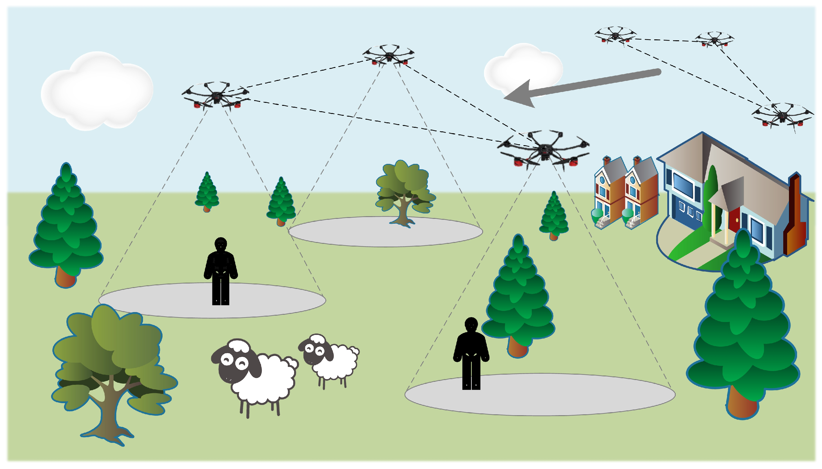
2.1. System Overview

As illustrated in Figure 2, this study focuses on UAV formation operations in collaborative scenarios, which include, but are not limited to, coordinated target tracking, synchronized supply drops, joint inspections, and collaborative strikes [20,21]. In such scenarios, UAV formations are required to arrive at specified task points in coordination (synchronously) to meet mission demands, ensure real-time task execution, and enhance overall efficiency.

Building on the assumption that flight path planning and task allocation for the UAV formation have already been completed, this study investigates flight energy consumption and synchronized arrival within UAV formations to support these collaborative operations. For clarity, we have compiled the symbols used in this paper along with their meanings, as shown in

Table 1. Explanation of symbols and their meanings.

Symbol	Meaning
$v_{opt}$	Optimal flight speed of UAV
${\tilde{v}}_i$	Initial velocity of UAV-i
$a_i$	Acceleration of UAV-i
$t_i$	Time for the UAV to accelerate from ${\tilde{v}}_i$ to $v_{opt}$
${\dot{t}}_i$	Time for UAV to fly at speed $v_{opt}$
${\ddot{t}}_i$	UAV hovering time
$T_i$	Flight time of UAV-i in each round of tasks
${\tilde{E}}_{i1}$	Energy consumption during flight at $v_{opt}$
${\tilde{E}}_{i2}$	Energy consumption during acceleration
${\ddot{E}}_i$	UAV hovering energy consumption
$T_i^s$	Total time spent by UAV in each task cycle
$E_i$	Total energy consumption of the UAV-i
$n_M$	Total task rounds
k	Task round index

.

2.2. UAV Energy Consumption Model

We take rotorcraft UAVs as the research background and derive their energy consumption during motion. When the UAV flies at a speed of v, its propulsion power is given by Equation (1) [22].

$$P\left(v\right)=p_0\left({\displaystyle \frac{3v^2}{U_{tip}^2}}\right)+p_i{\left(\sqrt{1+{\displaystyle \frac{v^4}{4v_0^4}}}-{\displaystyle \frac{v^2}{2v_0^2}}\right)}^{{\displaystyle \frac{1}{2}}}+{\displaystyle \frac{d_0\rho sA{v}^3}{2}}$$

(1)

where $d_0$ denotes the body drag ratio, s represents rotor stiffness, and $\rho$ and A refer to air density and rotor disk area, respectively. The terms $p_0$ and $p_i$ indicate the profile power and induced power of the blades in a hovering state, while $U_{tip}$ signifies the rotor tip speed and $v_0$ represents the average rotor induced speed in a hovering condition. The values of $p_0$ and $p_i$ are constants, and their specific meanings can be referenced in Equation (3).

Let the optimal flight speed of the UAV during level flight be denoted as $v_{opt}$. The initial speed and acceleration of UAV-i are represented as ${\tilde{v}}_i$ and $a_i$, respectively. The time it takes for the UAV to accelerate from ${\tilde{v}}_i$ to $v_{opt}$ is given by $t_i$, and the time spent flying at speed $v_{opt}$ is denoted as ${\dot{t}}_i$. Thus, $v_{opt}\left(t_i\right)={\tilde{v}}_i+a_i{t}_i$, and the total flight time can be expressed as $T_i=t_i+{\dot{t}}_i$.

Consequently, the energy consumption during the level flight phase is represented as ${\tilde{E}}_{i1}={\dot{t}}_{i}P\left(v_{opt}\right)$. Correspondingly, let the total flight energy consumption be defined as ${\tilde{E}}_i={\tilde{E}}_{i1}+{\tilde{E}}_{i2}$. The energy consumption during the acceleration phase ${\tilde{E}}_{i2}$ can be expressed as the integral of the instantaneous power $P\left(v\right)$ over the flight time $t_i$ and computed using Equation (2).

$${\tilde{E}}_{i2}={\int }_0^{t_i}P\left(v_i\left(t\right)\right)dt$$

(2)

Due to the inconsistency in the task execution times of different UAVs within their respective task areas, it is necessary for some UAVs to maintain a hover in order to ensure the consistency of the UAV formation’s arrival. When a UAV is in a hovering state, its velocity is $v=0$, and its power consumption depends on the rotor disk area and the aircraft’s weight. The hovering power consumption can be modeled as Equation (3).

$$P_h=p_0+p_i=\underset{P_0}{\underbrace{{\displaystyle \frac{\zeta }{8}}\rho sA{\mathsf{\Omega }}^3{R}_r^3}}+\underset{P_i}{\underbrace{\left(1+k_1\right){\displaystyle \frac{W_U^{3/2}}{\sqrt{2\rho A}}}}}$$

(3)

where $\zeta$ denotes the blade profile drag coefficient, $\mathsf{\Omega }$ represents the rotational speed of the rotor, $R_r$ indicates the radius of the rotor, $k_1$ is the induced power correction coefficient, and $W_U$ signifies the mass of the UAV.

Assuming that the hovering time of UAV-i is ${\ddot{t}}_i$ and the hovering energy consumption is ${\ddot{E}}_i={\ddot{t}}_i{P}_h$, the total time taken by UAV-i to fly a distance of $d_i$ and hover for ${\ddot{t}}_i$ is $T_i^s=T_i+{\ddot{t}}_i$, and the corresponding total energy consumption is $E_i={\tilde{E}}_i+{\ddot{E}}_i$.

2.3. Energy Consumption Optimization and Coordinated Arrival Model for UAV Formation

In this context, we introduce the concept of task rounds, with a total of $n_M$ task rounds. In the k-th task round, where $k\in \{1,2,\cdots ,n_M\}$, the UAV formation is required to arrive at the task point simultaneously, optimizing either flight energy consumption or flight speed to undertake the corresponding tasks. Furthermore, we establish a cooperative arrival evaluation model for UAVs, as follows:

When the number of UAVs in the formation is $n_u$, for coordinated arrival, all UAVs must arrive at the target as simultaneously as possible. The time difference of arrival between any two UAVs, denoted as $T^c$, is described by a mathematical model as Equation (4).

$$T_{ij}^c=\left|T_i^s-T_j^s\right|,\forall i,j\in \left\{1,2,\cdots ,n_u\right\},i\ne j$$

(4)

Correspondingly, the time difference for the UAV formation to arrive at the designated target is given by Equation (5).

$$f_1=\sum _{i=1}^{n_u}\sum _{j=1}^{n_u}{T}_{ij,k}^c$$

(5)

To evaluate the energy efficiency of the UAV formation during flight, the energy cost is calculated using Equation (6).

$$f_2=\sum _{i=1}^{n_u}{E}_{ik}$$

(6)

Letting $F=\left(f_1,f_2\right)$, the optimization model for UAV formation energy consumption and collaborative arrival is established as in Equation (7).

$$\begin{array}{cc}\hfill & \mathrm{P}1:\underset{v_{ik},t_{ik},{\dot{t}}_{ik},{\ddot{t}}_{ik},v_{opt}}{min}:F\left(d_{ik}\right)\hfill \\ \hfill & \mathrm{s}.\mathrm{t}.\hfill \\ \hfill & \forall i\in \left\{1,2,\cdots ,n_u\right\},\forall k\in \left\{1,2,\cdots ,n_m\right\},a_{ik}\in [a_m,a_M],v_{ik}\in [0,v_M],\{t_{ik},{\dot{t}}_{ik},{\ddot{t}}_{ik}\}\ge 0\hfill \\ \hfill & d_{ik}={\tilde{v}}_{ik}{t}_{ik}+a_{ik}{t}_{ik}^2/2+{\dot{t}}_{ik}{v}_{opt}\hfill \end{array}$$

(7)

The above equation indicates that in each round of the task, given the flight distance, the goal is to determine the acceleration time $t_{ik}$, optimal cruising speed $v_{opt}$, cruising flight time ${\dot{t}}_{ik}$, hovering time ${\ddot{t}}_{ik}$, and real-time flight speed $v_{ik}$ for each UAV, such that the UAV formation minimizes flight energy consumption and the time difference of arrival during the flight process. The constraints limit the ranges of UAV acceleration, speed, and hovering time, where $d_{ik}$ represents the distance of UAV-i from the task point in the k-th round of the task.

2.4. Model Processing

It is evident that $\mathrm{P}1$ represents a non-convex multi-objective optimization problem with equality constraints. Furthermore, P1 includes multiple decision variables, leading to a significant increase in problem dimensionality as the length of the UAV trajectory or the size of the UAV formation increases, which in turn substantially escalates the demand for computational resources. To address this issue, this study reconstructs the aforementioned model, simplifying the problem’s dimensionality while transforming the multi-objective optimization problem into a single-objective one for solving, thereby reducing computational complexity and enhancing algorithmic efficiency.

First, regarding Equation (1) and Equation (2), due to the presence of double square root operations in Equation (1), it is challenging to obtain an analytical solution for the integral operation in Equation (1). Therefore, utilizing a first-order Taylor expansion, we have $\sqrt{1+x}\approx 1+x/2$. When $\left|x\right|\ll 1$, Equation (1) can be approximated as a convex function, as shown in Equation (8).

$$P\left(v\right)\approx p_0\left({\displaystyle \frac{3v^2}{U_{tip}^2}}\right)+p_i{\displaystyle \frac{v_0}{v}}+{\displaystyle \frac{d_0\rho sA{v}^3}{2}}$$

(8)

By substituting Equation (8) into Equation (2), the analytical solution for ${\tilde{E}}_{i2}$ is obtained, as shown in Equation (9).

$$\begin{array}{cc}\hfill & {\tilde{E}}_{i2}\approx {\int }_0^{t_i}P\left(v_i\left(t\right)\right)dt={\int }_0^{t_i}\left({\displaystyle \frac{3p_0{\left({\tilde{v}}_i+a_{i}t\right)}^2}{U_{tip}^2}}\right)+{\displaystyle \frac{p_i{v}_0}{{\tilde{v}}_i+a_i{t}_i}}+{\displaystyle \frac{d_0\rho sA{\left({\tilde{v}}_i+a_{i}t\right)}^3}{2}}dt\hfill \\ \hfill & ={\displaystyle \frac{3p_0}{U_{tip}^2}}\left({\tilde{v}}_i^2{t}_i+a_i{\tilde{v}}_i{t}_i^2+{\displaystyle \frac{a_i^2{t}_i^3}{3}}\right)+{\displaystyle \frac{p_i{v}_0}{a_i}}\xi +{\displaystyle \frac{d_0\rho sA}{2}}\left({\tilde{v}}_i^3{t}_i+{\displaystyle \frac{3{\tilde{v}}_i^2{a}_i{t}_i^2}{2}}+{\tilde{v}}_i{a}_i^2{T}_i^3+{\displaystyle \frac{a_i^3{t}_i^4}{4}}\right)\hfill \end{array}$$

(9)

where $\xi =ln\left({\displaystyle \frac{{\tilde{v}}_i+a_i{t}_i}{{\tilde{v}}_i}}\right)$. It is evident that this expression is valid only when $a_i\ne 0$ and ${\tilde{v}}_i\ne 0$. However, based on the properties of acceleration, when the acceleration time $t_i=0$, it implies that the acceleration $a_i=0$. Furthermore, when $a_i\to 0$, we have: ${lim}_{a_i\to 0}{\tilde{E}}_{i2}\left(a_i\right)\approx t_{i}P\left({\tilde{v}}_i\right)$. The aforementioned conclusions and numerical simulation results indicate a high degree of similarity between Equations (1) and (9).

Secondly, for the optimization of the overall arrival time of the UAV formation at the corresponding target, we can introduce the variable ${\tilde{T}}_k$, defined as ${\tilde{T}}_k=t_{ik}+{\dot{t}}_{ik}+{\ddot{t}}_{ik}$. In the k-th round of the task, it is assumed that all UAVs arrive at the corresponding task point simultaneously within ${\tilde{T}}_k$ time. By adjusting the values of $t_{ik},{\dot{t}}_{ik},{\ddot{t}}_{ik}$, the objective function can be set to $f_1=0$.

Clearly, the relationship between the hovering time and ${\tilde{T}}_k$ is given by ${\ddot{t}}_{ik}={\tilde{T}}_k-t_{ik}-{\dot{t}}_{ik}$.

Next, based on the relationship between acceleration and velocity, at time t, the flight speed of UAV-i can be calculated by Equation (10).

$$v_{ik}\left(t\right)=\left\{\begin{array}{c}{\tilde{v}}_i+a_{i}t,t\le t_i\hfill \\ v_{opt}\left(t_i\right),t>t_i\hfill \end{array}\right.$$

(10)

We obtain the expression for acceleration as $a_i={\displaystyle \frac{v_{opt}-{\tilde{v}}_i}{t_i}}$. Furthermore, when the path length is denoted by $d_i$, it can be expressed as $d_i={\tilde{v}}_i{t}_i+{\displaystyle \frac{1}{2}}{a}_i{t}_i^2+{\dot{t}}_i{v}_{opt}$.

The flight time ${\dot{t}}_i$ for UAV-i to fly at the energy-optimal speed $v_{opt}$ can be further calculated based on Equation (11).

$${\dot{t}}_i={\displaystyle \frac{d_i-\left({\tilde{v}}_i{t}_i+a_i{t}_i^2/2\right)}{v_{opt}}}$$

(11)

Therefore, the solution for the real-time flight speed $v_{ik}$ can be transformed into the problem of solving for the acceleration time $t_{ik}$ and the duration to reach the task point ${\tilde{T}}_k$. In summary, the cost function $f_2$ corresponding to the energy optimization problem of the UAV formation can be rewritten as Equation (12).

$$\begin{array}{cc}\hfill & \mathrm{P}2:\underset{{\tilde{T}}_k,t_{ik},v_{opt}}{min}:{\tilde{f}}_2\left({\tilde{v}}_{ik},d_{ik}\right)=\sum _{i=1}^{n_u}{E}_{ik}\left({\tilde{v}}_{ik},d_{ik}\right)\hfill \\ \hfill & \mathrm{s}.\mathrm{t}.\hfill \\ \hfill & \forall i\in \left\{1,2,\cdots ,n_u\right\},\forall k\in \left\{1,2,\cdots ,n_m\right\},a_{ik}\in [a_m,a_M],v_{ik}\in [0,v_M],\{t_{ik},{\dot{t}}_{ik},{\ddot{t}}_{ik}\}\ge 0\hfill \\ \hfill & d_{ik}={\tilde{v}}_{ik}{t}_{ik}+a_{ik}{t}_{ik}^2/2+{\dot{t}}_{ik}{v}_{opt}\hfill \end{array}$$

(12)

Equation (12) indicates that after obtaining the value of the flight distance $d_{ik}$, in the k-th step, the acceleration time $t_{ik}$ for each UAV, the optimal flight speed $v_{opt}$, and the duration ${\tilde{T}}_k$ for the formation to reach the corresponding task point are calculated. This is performed to minimize the energy consumption of the UAV formation while ensuring that all UAVs arrive simultaneously at the task area.

3. Algorithm Design for Solution

At this point, the multi-objective optimization problem P1 has been transformed into a single-objective optimization problem with equality and inequality constraints, denoted as problem P2, which can be solved to optimality using the interior-point method (IPM) [23].

Compared to traditional swarm intelligence algorithms, the interior-point method employs optimization techniques based on gradient and second-order information, typically exhibiting quadratic convergence. This means that as the solution approaches the optimal value, the convergence speed becomes very rapid.

Additionally, the interior-point method guarantees the attainment of a global optimal solution with high precision when handling convex optimization problems. However, during the solution process, it is necessary to estimate the initial values of the variables; the closer the initial values are to the final optimal solution, the greater the efficiency of the solution.

To this end, it can be assumed that each UAV is initially at the optimal flight speed ${\stackrel{⌢}{v}}_{opt}$ before departure, and the path length to the task point is $d_i$, resulting in a flight time of $d_i/v_{opt}$. Substituting this into Equation (8), the instantaneous flight energy consumption of the UAV is obtained, as shown in Equation (13).

$${\tilde{E}}_{i1}\left({\stackrel{⌢}{v}}_{opt}\right)=d_i\left(p_0\left({\displaystyle \frac{3{\stackrel{⌢}{v}}_{opt}}{U_{tip}^2}}\right)+p_i{\displaystyle \frac{v_0}{{\left({\stackrel{⌢}{v}}_{opt}\right)}^2}}+{\displaystyle \frac{d_0\rho sA{\left({\stackrel{⌢}{v}}_{opt}\right)}^2}{2}}\right)$$

(13)

Taking the derivative of $v_{opt}$, we have

$${\displaystyle \frac{d{\tilde{E}}_{i1}\left({\stackrel{⌢}{v}}_{opt}\right)}{d{v}_{opt}}}=d_i\left({\displaystyle \frac{3p_0}{U_{tip}^2}}-{\displaystyle \frac{2p_i{v}_0}{{\left({\stackrel{⌢}{v}}_{opt}\right)}^3}}+d_0\rho sA{\stackrel{⌢}{v}}_{opt}\right)$$

(14)

Setting Equation (14) to zero, then,

$$d_0\rho sA{\left({\stackrel{⌢}{v}}_{opt}\right)}^4+{\displaystyle \frac{3p_0{\left({\stackrel{⌢}{v}}_{opt}\right)}^3}{U_{tip}^2}}-2p_i{v}_0=0$$

(15)

At this point, the initial value of the optimal flight speed ${\stackrel{⌢}{v}}_{opt}$ can be obtained directly using algebraic solving tools.

Based on the model reconstruction and interior-point method optimization, the pseudocode for the UAV formation flight time synchronization and energy consumption optimization strategy is shown in Algorithm 1.

Algorithm 1 Optimization Algorithm Based on Model Reconstruction and IPM

$\mathbf{Input}$: $n_u,n_M,a_m,a_M,v_M$ represent the number of UAVs, total task rounds, minimum and maximum acceleration, and maximum speed. The UAV task point matrix is ${\mathbf{P}}_i^{3\times N_M}$, with convergence parameter $\epsilon$, maximum iterations $I_T$, and UAV parameters. Initialize task rounds $k=0$ and UAV initial velocity ${\tilde{v}}_i=0$.   Use Equation (15) to calculate the initial value of the optimal flight speed ${\stackrel{⌢}{v}}_{opt}$.    repeat-1        Calculate the distance between adjacent task points $d_{ik},i\in \{1,2,\dots ,n_u\}$.        $k=k+1$        repeat-2           Construct Lagrangian function based on Equation (13), compute KKT conditions.           Compute the gradient, feasibility, and complementary slackness conditions.           Start the iteration and use the Newton method to solve the KKT conditions.        until-2 The algorithm converges or reaches the maximum number of iterations.        Obtain the solution for $P2$ which includes $t_{ik}$, $v_{opt}$, ${\tilde{T}}_k$.        Subsequently, compute ${\dot{t}}_{ik}$, ${\ddot{t}}_{ik}$, and $a_{ik}$.        The initial speed of the UAV is ${\tilde{v}}_i=v_{opt}$.    until-1 $k=n_M$. $\mathbf{Output}$: $t_{ik}$, $v_{opt}$, ${\tilde{T}}_k$, ${\dot{t}}_{ik}$, ${\ddot{t}}_{ik}$, and $a_{ik}$, along with the flight energy consumption.

4. Simulation Experiment

Without loss of generality, we set the number of UAVs in formation, $n_u$, to 5. The UAV acceleration range is set to $[-10,10]{\mathrm{m}/\mathrm{s}}^2$, and the maximum UAV speed is set to $30\mathrm{m}/\mathrm{s}$. The remaining parameters are listed in

Table 2. Parameter setting.

Symbol	Meaning	Value
W	UAV weight/N	18
$R_r$	Rotor radius/m	0.4
$\rho$	Air density/kg/m2	1.225
A	Rotor disk area/m2	0.503
$v_0$	Average rotor-induced velocity in hovering/m/s	4.03
$U_{tip}$	Rotor tip speed m/s	120
$\zeta$	Profile resistance coefficient	0.012
$\mathsf{\Omega }$	Rotor speed rad/s	300
$k_1$	Inductive power correction coefficient	0.1
b	Number of blades	4
c	Blade chord length/m	0.0157
$S_F$	Equivalent plane area of fuselage/m2	0.151
$d_0$	Airframe drag ratio $d_0=S_F/\left(sA\right)$	0.6

The algorithm’s convergence parameter is $\epsilon =0.0001$ with a maximum of $I_T=1000$ iterations.

.

4.1. Experiment Scenario 1

With the above parameter settings, a UAV formation’s task area and flight trajectory in an environment with obstacles are randomly generated, as shown in Figure 3.

The dots in Figure 3 represent the UAVs’ respective task points, and the initial value of the optimal flight speed is determined according to Equation (15).

Additionally, the flight distance for each round of the UAV formation task is shown in Figure 4.

As shown in Figure 4, each UAV’s required flight distance varies per task round due to environmental interference and differing task point locations. In this scenario, each UAV in the formation needs to adjust its flight speed to ensure optimal energy consumption while achieving synchronous arrival at its designated task point.

By executing Algorithm 1, the time taken and total energy consumption for each task round of the UAV formation are obtained, as illustrated in Figure 5.

Based on Figure 4 and Figure 5, it can be concluded that as the distance of each task round increases, the time taken by the UAV formation for the task increases linearly, and the corresponding energy consumption also increases linearly. These results validate the effectiveness of the time and energy consumption model established in this study.

The changes in speed and acceleration for each UAV during every task round are determined, as shown in Figure 6.

From Figure 6, it can be observed that during each task round, each UAV calculates the distance to the task point and adjusts its acceleration to influence its flight speed, achieving coordinated arrival. When the UAV’s acceleration is positive, its speed increases linearly. Conversely, when the acceleration is negative, the corresponding speed decreases linearly, with the specific increase or decrease depending on the duration of the acceleration effect. Additionally, it is evident that the flight speed of each UAV during every task round is around 13 m/s, which is close to the initial value of the optimal speed calculated in Equation (15). This result demonstrates the effectiveness of the aforementioned model.

Furthermore, the changes in acceleration time and constant speed flight time for the UAV formation during each task round are presented in Figure 7.

From Figure 7a, it can be observed that the acceleration time for each UAV is very short (all within 0.5 s). However, Figure 6 shows that the instantaneous acceleration of the UAVs has essentially reached their maximum acceleration. This result can be explained by Equation (9), which indicates that the power of acceleration time is greater than that of acceleration.

In other words, the impact of an increase in acceleration time on energy consumption is greater than that of an increase in acceleration. Additionally, Figure 7b illustrates a linear relationship between the duration of constant-speed flight time and the flight distance in each task round.

It is noteworthy that, in the experimental environment described, the hovering time for each UAV is zero. There are two main reasons for this. Firstly, when the UAV flies at a nearby speed, the energy consumption per unit time during hovering is higher than that during propulsion. Secondly, compared to propulsion energy consumption, hovering energy consumption adds extra energy costs to task execution. Therefore, in order to ensure coordinated arrival, it is essential to avoid increasing hovering energy consumption as much as possible.

4.2. Experiment Scenario 2

To further validate the effectiveness of the model, this study additionally simulates the variation in hovering time when the UAV formation cannot achieve coordinated arrival by adjusting acceleration, flight speed, and corresponding time.

The details are as follows.

We consider the flight trajectory of the UAV formation shown in Figure 8. It is assumed that the UAV formation encounters disturbances during flight, prompting evasive measures that disrupt the formation.

In this study, the focus is not on modeling the environmental interference itself but rather on addressing the consequences of such interference on the UAV formation. Specifically, we investigate how to achieve coordinated arrival when the UAV formation experiences disruptions caused by external disturbances.

For simplicity, the interference is assumed to result in deviations from the planned trajectory and formation. The subsequent analysis focuses on how the UAV formation can adjust acceleration, flight speed, and timing to mitigate the effects of these deviations and reestablish coordination. This approach allows us to emphasize the proposed methodology for coordinated arrival under disrupted conditions rather than delve into the detailed modeling of the interference source. Future work may include a more comprehensive exploration of interference models and their integration with the current framework.

As shown in Figure 8, at the end of the trajectory, the UAV formation appears relatively dispersed, which requires some UAVs to hover in order to ensure coordinated arrival of the formation.

Then, by running Algorithm 1, the hovering time corresponding to each round of tasks along the above trajectory is obtained, as shown in Figure 9.

From Figure 9, it can be observed that as the degree of trajectory dispersion increases, some UAVs in the formation begin to utilize hovering to ensure coordinated arrival. This further demonstrates the effectiveness of the related model and solution algorithm.

4.3. Algorithm Performance Test

To verify the performance of the solution algorithm, the convergence of the objective function and the constraints during the solving process was statistically analyzed, with results shown in Figure 10.

The above results were obtained under the parameters of experimental Scenario 2.

From Figure 10, it can be seen that the algorithm described in this paper achieved convergence by the 18th iteration, demonstrating high solving efficiency. Additionally, when the initial value of the optimal flight speed, ${\stackrel{⌢}{v}}_{opt}$, is set to 0, the number of iterations required for the algorithm to achieve convergence of the objective function and constraints under the same parameters increases to 67. This further illustrates the effectiveness and importance of the initial value estimation method discussed in Section 3.

To further validate the proposed method’s computational performance in handling different UAV formation trajectories, we designed experiments involving five UAVs with distinct flight paths, corresponding to scenarios with varying total task rounds (TTRs). The experiments were conducted on a desktop computer equipped with an Intel i5-12400F CPU, 16 GB of memory, and the Windows 10 operating system. The computation time for solving each task round was recorded, and the average task computation time (ATC) for different trajectories is shown in Figure 11.

The results demonstrate that the proposed method can effectively optimize the energy consumption and collaborative arrival of the five UAVs. Notably, the ATC remains stable at approximately 70 ms per task round, regardless of changes in the total task rounds, indicating its applicability for real-world scenarios.

To further demonstrate the superiority of the proposed method, we conducted a comparative study against two widely recognized algorithms: the Moth Flame Optimization (MFO) [24] algorithm and the Improved Grey Wolf Optimization (IGWO) [25] algorithm. These benchmark algorithms have been extensively applied and validated in various engineering fields [26,27]. In the experiments, the population size for MFO and IGWO was set to 30.

Under identical environmental conditions and system configurations, we conducted performance tests focusing on the solution accuracy and efficiency of the algorithms.

Firstly, we evaluated the solution accuracy of three algorithms when applied to the same UAV formation trajectory. Specifically, accuracy is reflected in the fitness values of the objective function calculated in each iteration. A smaller fitness value indicates higher solution accuracy. The UAV formation trajectories and the fitness values of the objective function for each algorithm across all iterations are shown in Figure 12.

As illustrated in Figure 12, while the fitness values achieved by the three algorithms appear similar for each task, a statistical analysis over 38 tasks reveals that the proposed algorithm reduced the average fitness value by 4.9% compared to the IGWO algorithm and by 6.6% compared to the MFO algorithm. Furthermore, the maximum difference in fitness values achieved by the proposed algorithm compared to IGWO and MFO reached 20.27% and 18.32%, respectively. These results highlight the improved accuracy of the proposed algorithm.

Secondly, to verify the computational efficiency of the algorithms as the size of the UAV formation increases, we evaluated the average computation time per task for different UAV formation sizes. The results are presented in Figure 13.

As shown in Figure 13, for formations with up to 10 UAVs, all three algorithms completed their calculations within 200 ms. However, as the formation size increased, the computation time exhibited a nearly exponential growth. When the formation size reached 50 UAVs, the proposed algorithm achieved an average computation time of 555 ms per task, compared to 691 ms for IGWO and 786 ms for MFO. This represents a reduction of up to 19.68% and 29.37%, respectively, further validating the efficiency and superiority of the proposed method.

5. Conclusions

This study focuses on addressing the critical challenges of collaborative arrival and energy consumption optimization in UAV formations by developing a comprehensive model and proposing effective solution strategies. Extensive simulation experiments were conducted to validate the feasibility and performance of the proposed model and algorithms. The validation process included analyses of linear relationships, speed and acceleration dynamics, acceleration and constant-speed flight time distributions, hovering scenarios, and algorithmic performance.

The experimental results demonstrate the high accuracy of the proposed model and the superior computational efficiency of the algorithm across various test scenarios. Notably, the proposed method outperforms benchmark algorithms in terms of computation time, particularly under larger UAV formation scales. These findings confirm the ability of the proposed approach to effectively address the challenges of UAV formation collaborative arrival and energy consumption optimization.

Future research will focus on implementing the proposed methods on UAV platforms and conducting field tests to evaluate their practical applicability in real-world scenarios.

References

1. Ouyang, Q.; Wu, Z.; Cong, Y.; Wang, Z. Formation control of unmanned aerial vehicle swarms: A comprehensive review. Asian J. Control 2023, 25, 570–593. [Google Scholar] [CrossRef]
2. Liu, Z.; Li, J. Application of unmanned aerial vehicles in precision agriculture. Agriculture 2023, 13, 1375. [Google Scholar] [CrossRef]
3. Cheng, N.; Wu, S.; Wang, X.; Yin, Z.; Li, C.; Chen, W.; Chen, F. AI for UAV-assisted IoT applications: A comprehensive review. IEEE Internet Things J. 2023, 10, 14438–14461. [Google Scholar] [CrossRef]
4. Luo, Q.; Luan, T.H.; Shi, W.; Fan, P. Edge computing enabled energy-efficient multi-UAV cooperative target search. IEEE Trans. Veh. Technol. 2023, 72, 7757–7771. [Google Scholar] [CrossRef]
5. Yasin, J.N.; Mohamed, S.A.S.; Haghbayan, M.H.; Heikkonen, J.; Tenhunen, H.; Yasin, M.M.; Plosila, J. Energy-efficient formation morphing for collision avoidance in a swarm of drones. IEEE Access 2020, 8, 170681–170695. [Google Scholar] [CrossRef]
6. Falkowski, K.; Duda, M. Dynamic models identification for kinematics and energy consumption of rotary-wing UAVs during different flight states. Sensors 2023, 23, 9378. [Google Scholar] [CrossRef]
7. Chen, L.; Xiao, J.; Lin, R.C.H.; Feroskhan, M. Angle-constrained formation maneuvering of unmanned aerial vehicles. IEEE Trans. Control Syst. Technol. 2023, 31, 1733–1746. [Google Scholar] [CrossRef]
8. Shao, X.; Liu, H.; Zhang, W.; Zhao, J.; Zhang, Q. Path driven formation-containment control of multiple UAVs: A path-following framework. Aerosp. Sci. Technol. 2023, 135, 108168. [Google Scholar] [CrossRef]
9. Gao, Y.; Qiao, Z.; Pei, X.; Wu, G.; Bai, Y. Design of energy-management strategy for solar-powered UAV. Sustainability 2023, 15, 14972. [Google Scholar] [CrossRef]
10. Ma, B.; Liu, Z.; Jiang, F.; Zhao, W.; Dang, Q.; Wang, X.; Zhang, J.; Wang, L. Reinforcement learning based UAV formation control in GPS-denied environment. Chin. J. Aeronaut. 2023, 36, 281–296. [Google Scholar] [CrossRef]
11. Wu, Y.; Liang, T.; Gou, J.; Tao, C.; Wang, H. Heterogeneous mission planning for multiple UAV formations via metaheuristic algorithms. IEEE Trans. Aerosp. Electron. Syst. 2023, 59, 3924–3940. [Google Scholar] [CrossRef]
12. Hu, W.; Yu, Y.; Liu, S.; She, C.; Guo, L.; Vucetic, B.; Li, Y. Multi-UAV coverage path planning: A distributed online cooperation method. IEEE Trans. Veh. Technol. 2023, 72, 11727–11740. [Google Scholar] [CrossRef]
13. Li, J.; Xiong, Y.; She, J. UAV path planning for target coverage task in dynamic environment. IEEE Internet Things J. 2023, 10, 17734–17745. [Google Scholar] [CrossRef]
14. Gong, S.; Wang, M.; Gu, B.; Zhang, W.; Hoang, D.T.; Niyato, D. Bayesian optimization enhanced deep reinforcement learning for trajectory planning and network formation in multi-UAV networks. IEEE Trans. Veh. Technol. 2023, 72, 10933–10948. [Google Scholar] [CrossRef]
15. Na, Y.; Li, Y.; Chen, D.; Yao, Y.; Li, T.; Liu, H.; Wang, K. Optimal energy consumption path planning for unmanned aerial vehicles based on improved particle swarm optimization. Sustainability 2023, 15, 12101. [Google Scholar] [CrossRef]
16. Souto, A.; Alfaia, R.; Cardoso, E.; Araújo, J.; Francês, C. UAV path planning optimization strategy: Considerations of urban morphology, microclimate, and energy efficiency using Q-learning algorithm. Drones 2023, 7, 123. [Google Scholar] [CrossRef]
17. Abubakar, A.I.; Ahmad, I.; Omeke, K.G.; Ozturk, M.; Ozturk, C.; Abdel-Salam, A.M.; Imran, M.A. A survey on energy optimization techniques in UAV-based cellular networks: From conventional to machine learning approaches. Drones 2023, 7, 214. [Google Scholar] [CrossRef]
18. Liang, Z.; Li, Q.; Fu, G. Multi-UAV Collaborative Search and Attack Mission Decision-Making in Unknown Environments. Sensors 2023, 23, 7398. [Google Scholar] [CrossRef]
19. Bu, Y.; Yan, Y.; Yang, Y. Advancement Challenges in UAV Swarm Formation Control: A Comprehensive Review. Drones 2024, 8, 320. [Google Scholar] [CrossRef]
20. Alhafnawi, M.; Salameh, H.A.B.; Masadeh, A.E.; Al-Obiedollah, H.; Ayyash, M.; El-Khazali, R.; Elgala, H. A survey of indoor and outdoor UAV-based target tracking systems: Current status, challenges, technologies, and future directions. IEEE Access 2023, 11, 68324–68339. [Google Scholar] [CrossRef]
21. Pan, Y.; Li, L.; Qin, J.; Chen, J.J.; Gardoni, P. Unmanned aerial vehicle–human collaboration route planning for intelligent infrastructure inspection. Comput. Civ. Infrastruct. Eng. 2024, 39, 2074–2104. [Google Scholar] [CrossRef]
22. Zeng, Y.; Xu, J.; Zhang, R. Energy minimization for wireless communication with rotary-wing UAV. IEEE Trans. Wirel. Commun. 2019, 18, 2329–2345. [Google Scholar] [CrossRef]
23. Rao, Y.; Su, J.; Kheirfam, B. A Full-Newton Step Interior-Point Method for Weighted Quadratic Programming Based on the Algebraic Equivalent Transformation. Mathematics 2024, 12, 1104. [Google Scholar] [CrossRef]
24. Sahoo, S.K.; Kumar, S.; Mohapatra, S.S.; Mistry, K. Moth Flame Optimization: Theory, Modifications, Hybridizations, and Applications. Arch. Comput. Methods Eng. 2023, 30, 391–426. [Google Scholar] [CrossRef] [PubMed]
25. Nadimi-Shahraki, M.H.; Taghian, S.; Mirjalili, S. An Improved Grey Wolf Optimizer for Solving Engineering Problems. Expert Syst. Appl. 2021, 166, 113917. [Google Scholar] [CrossRef]
26. Reddy, M.R.; Kumar, K.; Narayana, K. Energy-Efficient Cluster Head Selection in Wireless Sensor Networks Using an Improved Grey Wolf Optimization Algorithm. Computers 2023, 12, 35. [Google Scholar] [CrossRef]
27. Vashishtha, G.; Kumar, R. An Amended Grey Wolf Optimization with Mutation Strategy to Diagnose Bucket Defects in Pelton Wheel. Measurement 2022, 187, 110272. [Google Scholar] [CrossRef]
Figure 1. Classification of UAV formation research.
Drones 08 00722 g001
Figure 2. Schematic diagram of UAV formation task scene.
Drones 08 00722 g002
Figure 3. Schematic diagram of UAV formation flight path and task point (3D)—Scenario 1.
Drones 08 00722 g003
Figure 4. Flight distance of UAVs.
Drones 08 00722 g004
Figure 5. Flight time and total energy consumption of UAV formation. (a) Time of flight. (b)Total energy consumption of UAV formation.
Drones 08 00722 g005
Figure 6. UAV formation flight acceleration and velocity changes. (a) UAV−1. (b) UAV−2. (c) UAV−3. (d) UAV−4. (e) UAV−5.
Drones 08 00722 g006
Figure 7. Statistical results of UAV formation flight time. (a) Acceleration time. (b) Constant speed flight time.
Drones 08 00722 g007
Figure 8. Schematic diagram of UAV formation flight path and task point (2D)—Scenario 2.
Drones 08 00722 g008
Figure 9. UAV hovering time.
Drones 08 00722 g009
Figure 10. Convergence of the objective function and constraint conditions.
Drones 08 00722 g010
Figure 11. Average computation time under different uav formation trajectories. TTR: total task rounds; ATC: average computation time.
Drones 08 00722 g011
Figure 12. The trajectory of the UAV formation and the change in the corresponding objective function fitness value.
Drones 08 00722 g012
Figure 13. Comparison of algorithm running time for different numbers of UAVs. (Left): UAV flight trajectories corresponding to different numbers of UAVs; (Right): Comparison of running time for different algorithms.
Drones 08 00722 g013