Multi-Phase Trajectory Planning for Wind Energy Harvesting in Air-Launched UAV Swarm Rendezvous and Formation Flight

Abstract

Small air-launched unmanned aerial vehicles (UAVs) face challenges in range and endurance due to their compact size and lightweight design. To address these issues, this paper introduces a multi-phase wind energy harvesting trajectory planning method designed to optimize the onboard electrical energy consumption during rendezvous and formation flight of air-launched fixed-wing swarms. This method strategically manages gravitational potential energy from air-launch deployments and harvests wind energy that aligns with the UAV’s flight speed. We integrate wind energy harvesting strategies for single vehicles with the spatial–temporal coordination of the swarm system. Considering the wind effects into the trajectory planning allows UAVs to enhance their operational capabilities and extend mission duration without changes on the vehicle design. The trajectory planning method is formalized as an optimal control problem (OCP) that ensures spatial–temporal coordination, inter-vehicle collision avoidance, and incorporates a 3-degree of freedom kinematic model of UAVs, extending wind energy harvesting trajectory optimization from an individual UAV to swarm-level applications. The cost function is formulized to comprehensively evaluate electrical energy consumption, endurance, and range. Simulation results demonstrate significant energy savings in both low- and high-altitude mission scenarios. Efficient wind energy utilization can double the maximum formation rendezvous distance and even allow for rendezvous without electrical power consumption when the phase durations are extended reasonably. The subsequent formation flight phase exhibits a maximum endurance increase of 58%. This reduction in electrical energy consumption directly extends the range and endurance of air-launched swarm, thereby enhancing the mission capabilities of the swarm in subsequent flight.

1. Introduction

The deployment of unmanned aerial vehicle (UAV) swarms is emerging as a future trend in UAV utilization as a single UAV cannot handle the demands of complex missions [1,2]. Deploying UAV swarms from multiple mother planes at varying altitudes makes it difficult to maintain appropriate vertical and horizontal spacing for the swarm formation. Additionally, the flight speed and safe distance of these mother planes are relatively large compared to the deployed UAVs’ speed, causing the UAVs to spread in a broad area. The air-launched UAVs can load limited fuel or battery capacity due to their compact size, lightweight design, and slow speed. This disadvantage impacts their endurance and capability to complete long-distance swarm missions. For instance, the endurance of reported UAV models, such as the U.S. Coyote and the Switchblade, is limited to approximately 30 min and 15 min, respectively [3,4]. Consequently, achieving rendezvous and formation flight in a broad area would consume a significant portion of their onboard electrical energy without trajectory optimization. In the wind field similar to their speed, the restricted range and endurance of these small, air-launched UAVs imply that relying exclusively on electrical power for achieving rendezvous can severely affect the performance of subsequent mission tasks [5]. Therefore, developing a method to enable these UAVs to rendezvous and maintain a formation with optimal energy consumption is crucial for the success of such missions [6]. This optimization is essential for maximizing the operational effectiveness of these swarms in complex mission scenarios.

Air-launched UAVs have a large reserve of gravitational potential energy when deployed from a mother plane. For small UAVs, this electrical energy cannot be replenished without in-flight refueling or charging, making the ability to harvest energy enroute crucial for extending their operational range and endurance. There are three approaches for in-flight energy harvesting, solar energy, thermal soaring, and dynamic soaring [7]. Applying solar energy harvesting to small air-launched UAVs presents several challenges, including the high costs associated with solar systems, limited wing area that restricts the installation of panels, insufficient power generation, and the short mission endurance that cannot guarantee adequate sunlight exposure. Thermal soaring involves converting the kinetic energy of rising air flow into gravitational potential energy for the UAV. This approach is generally limited to daytime operations and is challenging to model quantitatively at high altitudes, as indicated by meteorological studies [8]. Dynamic soaring exploits horizontal wind gradients in the vertical direction to counteract aerodynamic drag, enabling sustained, non-powered flight [9]. For small UAVs, harnessing the energy from wind gradients offers the potential for biomimetic, long-endurance flights, making it a particularly promising approach [10,11,12].

Recent research in the field of wind energy harvesting trajectories has focused on optimizing the flight strategies of a single UAV engaged in dynamic soaring, rather than addressing the swarm systems. Dynamic soaring trajectories can be “open-loop”, where the UAV soars forward in a specific direction, or “closed-loop”, where it loiters near a fixed point [7,13]. Recent advancements include mini-UAVs, typically around 10 kg, utilizing dynamic soaring to significantly extend their flight distance and endurance [14]. Radio-controlled gliders leveraging dynamic soaring have achieved impressive speeds, with records now reaching up to 545 mph [9]. This method allows UAVs to traverse large distances and achieve high speeds without consuming mechanical or electrical energy [15]. The efficiency of energy harvesting is highly dependent on the UAVs’ parameters and prevailing wind conditions [16]. Achieving the necessary conditions for energy-neutral dynamic soaring remains a significant challenge [17,18]. Sachs, Zhao, and Qi have explored the use of low wind gradients to minimize electrical energy use and the implementation of powered-augmented dynamic soaring to enhance efficiency [19,20]. The associated costs of these trajectory planning methods include factors such as minimum thrust, average power, and energy loss.

The field of UAV swarm trajectory planning currently lacks research focused on wind energy harvesting. This research can be divided into two sub-problems, the spatial–temporal coordination of the swarm and power-augmented wind energy harvesting flight. In the realm of optimal path or trajectory planning, existing methods are generally classified into three categories as follows: geometry-based method, intelligent optimization algorithms, and optimal control methods [21,22]. The geometry-based method is questionable, as whether the polynomial trajectories generated can be successfully tracked by fixed-wing UAVs remains a problem [23]. The intelligent optimization algorithm, characterized by inherent randomness, overwhelmingly generates numerous infeasible trajectories during convergence which consume high computation that hinder their applications in efficiency-critical scenarios. The optimal control method is a suitable approach for swarm trajectory planning, involving a complex kinematic model, and it is prevalent in planning for optimal energy research. Solutions derived from the optimal control method tend to be more accurate and feasible as they conform to the UAV kinematic model and include the cooperative and coordinative constraints of the swarm system [24]. In the research including thrust or power as a control variable, a critical oversight in the formulation of these Optimal Control Problems (OCPs) is the consideration of only the saturation constraints of control variables, neglecting the limitations on their rate of increment. This oversight can lead to untraceable trajectories due to discontinuities in control input, which do not align with the actual characteristics of the control system [11,25]. A possible solution is to introduce control increment as virtual control variables, which allows for the implementation of increment rate constraints without the need to introduce new variables. This approach requires only the addition of state variables and equations, incorporating the first-order system response to control input, thus maintaining the existing trajectory planning methodology.

The OCP method emerges as a powerful tool for formulating wind energy harvesting trajectory planning for air-launched UAV swarms. This approach enables the straightforward implementation of constraints on the rate of change in control variables and incorporates a comprehensive cost function [26]. Several software packages have been developed to numerically solve OCP [27,28,29,30], broadly categorized into indirect and direct methods. Indirect methods, while theoretically sound, often encounter difficulties when dealing with complex inequality or equality constraints, limiting their practicality for optimal trajectory problems involving multiple constraints, as is common in UAV swarm scenarios [31]. Conversely, direct methods convert the OCP into a static Nonlinear Programming Problem (NLP). This transformation involves applying dynamic constraints at discrete points, using various quadrature rules to facilitate the easier management of constraints [32,33]. Direct methods are also characterized by their low sensitivity to initial conditions and a wide radius of convergence, making them particularly suitable for optimal control planning [34]. Among the direct methods, the pseudo-spectral method has gained significant attention [35]. The hp-adaptive pseudo-spectral method, in particular, has been extensively applied to the optimal trajectory planning of multiple vehicles, demonstrating its capability to match the optimality and efficiency of indirect methods. Ongoing research continues to enhance the performance of the hp-adaptive pseudo-spectral method [36]. Their results indicate that the GPM-based planning method can be effectively integrated in the onboard systems. This progress underscores the ongoing advancements in OCP solutions and their critical role in enhancing the operational capabilities of UAV swarms [37,38].

A review of the literature indicates a research gap in the modeling of multi-phase trajectories for wind energy harvesting in UAV swarms, particularly in the integration of spatial–temporal coordination with wind energy harvesting strategies. There is a need for studies that investigate how individual vehicles can harvest wind energy to achieve optimal swarm trajectories while complying with the spatial–temporal constraints of multiple UAVs. Limited research exists on enhancing trajectory algorithm performance by introducing a thrust increment as a virtual control variable, which could reduce the number of adaptive collocation points required to solve individual trajectories within the swarm’s OCP trajectory planning. Additionally, there is a paucity of quantitative analysis on the impact of optimal multi-phase trajectory planning for swarms utilizing wind energy on the endurance and cost-effectiveness of these trajectories.

To our knowledge, there is no relevant research on the multi-phase trajectory optimization of UAV swarms which comprehensively considers the spatial–temporal coordination of the swarm system and the optimal trajectory for wind energy harvesting. This paper addresses this gap by proposing a multi-phase trajectory planning method that optimizes flight time, electrical energy consumption, and formation position during the rendezvous and formation flight of air-launched swarms. The proposed method incorporates wind energy harvesting trajectories that combine sequentially connected open-loop and closed-loop trajectory components, tailored to different mission scenarios. By effectively managing gravitational potential energy reserves from air-launched deployment and harvesting wind energy that aligns with the UAV’s flight speed, it optimizes the use of potential, electrical, wind, and kinetic energies in relation to specific wind conditions. This research focuses on air-launched, fixed-wing swarm systems and explores multi-phase wind energy harvesting trajectories with an integrated spatial–temporal coordination, effectively extending wind energy harvesting strategies from single UAVs to the swarm level. Unlike previous studies which focus on simpler trajectory models or single UAV scenarios, this paper integrates continuous constraints of multi-phase trajectories through the hp-adaptive pseudo-spectral method and incorporates a comprehensive kinematic model based on 3 Degrees of Freedom (3DOF) for each UAV. The spatial–temporal coordination among the swarm members is defined as path constraints in an OCP model. The inter-vehicle collision avoidance is formulated as inequality constraints, while the initial and final times and positions for each phase are treated as equality constraints. By optimizing the trajectory planning for swarm rendezvous and formation flight, this approach significantly reduces electrical energy consumption during these critical phases of the mission.

The rest of this paper is organized as follows: Section 2 introduces the two-phase trajectory for air-launched UAVs in a mission scenario, as well as the models used for the UAV and wind. The OCP for wind energy harvesting trajectory planning of air-launched swarms are described, and its numerical method utilizing direct collocation method is formulated in Section 3. The solutions and discussions for low-altitude and high-altitude mission scenarios are presented in Section 4. Finally, the conclusions are drawn in Section 5.

2. Problem Formulation

2.1. Mission Scenario

Figure 1 illustrates a mission scenario where multiple UAVs are released from two mother planes at different time intervals and altitudes with a great reserve in gravitational potential energy. Each mother plane releases two UAVs that first execute a wind energy harvesting rendezvous trajectory (Phase 1) in wind conditions and then transition to a coordinated formation flight (Phase 2). Variations in the release timings and velocities of the mother planes lead to measurable horizontal and vertical separations between these UAVs at the initial state of deployment. Considering the significant speed of the mother planes, even a 2 s variation in release timing can extend the horizontal separation to over 200 m. Furthermore, the horizontal distance between UAVs in the swarm tends to increase with each subsequent individual deployment. Relying on onboard batteries for establishing formation in wind conditions results in significant electrical energy consumption which compromises the mission’s capability and feasibility. To minimize electrical energy loss for the rendezvous and formation phase in these scenarios, a wind energy harvesting rendezvous trajectory planning method is proposed.

2.2. Wind and UAV Model

The impact of wind on optimal trajectory planning varies based on the typical airspeed and category of the aircraft. For the flight of small UAVs, where their airspeed is close to the prevailing wind speeds, the range and endurance are affected significantly. This is a critical factor concerning the mission capability of air-launched small UAVs. The employed linear gradient wind and UAV model are presented.

Wind speed and direction are crucial for wind energy harvesting trajectory planning. Common wind field models include exponential, logarithmic, and linear types, with the first two having proved accuracy near the ground due to surface friction effects. Figure 2 illustrates a typical variation in horizontal wind speed with altitude, suggesting that within the altitude ranges of 1.1–0.5 km and 8.3–6 km, a linear wind model can approximate the wind speed effectively. The dash line represents the wind velocity profiles, while the solid line indicate the altitude ranges selected for this study. The specific wind speed values for these layers are detailed in

Table 1. Parameters of linear wind conditions [40].

Scenario	Altitude Range	Wind Magnitude	Wind Gradient
Low-altitude	1.1–0.5 km	7 m/s	0.016 s−1
High-altitude	8.3–6 km	20 m/s	0.016 s−1

. While the transient and spatial variability of the wind would not affect the OCP method, it influences the boundary conditions and time step of the rolling execution of the planning process. The unsteady wind can be represented as the change in steady wind in different discrete intervals. For the purpose of this study, it is assumed that the wind direction remains constant within these altitude ranges, aligning with the positive X-direction of the motion coordinate system during the mission period.

The utilized exponential atmospheric density model is as follows [41]:

$${\rho }_i={\rho }_0{e}^{-\beta R_{0}h}$$

(1)

where ${\rho }_0=1.225\mathrm{kg}/{\mathrm{m}}^3$ and $\beta =1/7201$.

The UAV model utilized is a foldable tandem-wing configuration, specifically designed for compact storage and transportation, optimized for air-launched deployment. Figure 3 shows its three views and axonometric perspective.

Table 2. Main parameters of the UAV.

Parameters	Value
$m$	20 kg
$g$	9.81 m/s2
Aspect Radio	11.5
$b$	1.8 m
$S$	0.58 m2

presents the main parameters of the UAV. The design prioritizes mission capabilities compared with common configurations for dynamic soaring that are aimed at maximizing wind energy harvesting efficiency. It incorporates lower lift-to-drag ratios and aspect ratios, complemented by a powerful propulsion system.

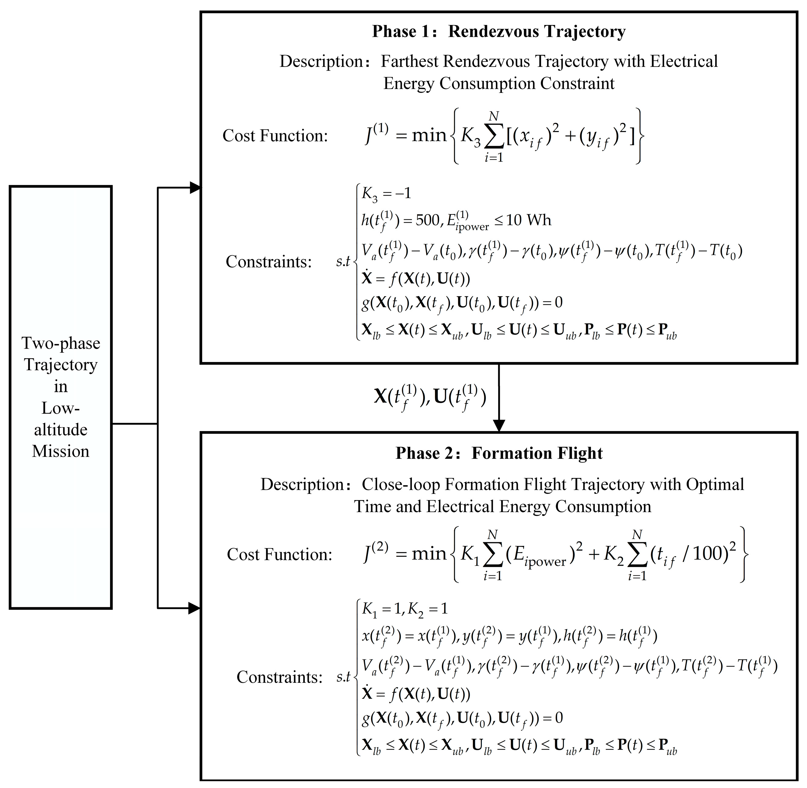
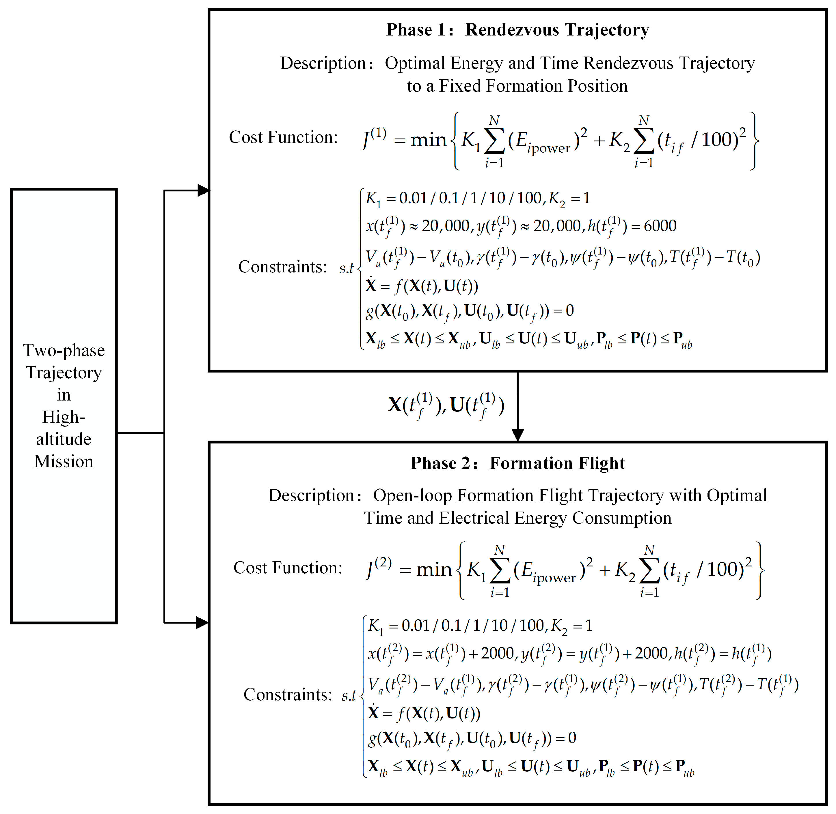
2.3. Optimal Control Model for the Multi-Phase Trajectory

To establish the OCP model for wind energy harvesting trajectories, a three-dimensional point mass model assuming a flat earth is sufficient [42]. The forces and angles acting on the UAV are depicted in Figure 4. The kinematic model, which incorporates thrust and wind influences, is formulated as Equation (2). This model includes terms for acceleration, velocity, and position, detailing interactions with its surrounding wind and the thrust [43].

The symbols used in the equations are defined as follows: $m$ is the mass, $V_{\mathrm{a}}$ is the airspeed, $V_w$ and ${\dot{V}}_w$ are the wind speed and its gradient, respectively. $V_{\mathrm{a}}$ denotes the UAV’s airspeed, which is the vector sum of the UAV’s ground speed ($V_e$) and the wind speed ($V_w$). This relationship of speeds is illustrated in Figure 4. $T$ is the thrust, $L$ is the lift, $D$ is the drag, $\gamma$ is the path angle, $\psi$ is the heading angle, and $\phi$ is the bank angle. The angle between $T$ and $D$ is the angle of the attack and sideslip. During flight, these angles do not typically exceed 10°. Therefore, $T$ is assumed to be along the positive X-axis of the wind coordinate system, with the components of thrust along the Y and Z axis being neglected. $T$ and $D$ are simplified in the direction of the wind speed. $L$ is perpendicular to the drag.

$$\left\{\begin{array}{l}m{\dot{V}}_a=T-D-mg\sin \gamma +m{\dot{V}}_W\cos \gamma \cos \psi \\ m{V}_a\cos \gamma \dot{\psi }=L\sin \phi -m{\dot{V}}_W\sin \psi \\ m{V}_a\dot{\gamma }=L\cos \phi -mg\cos \gamma -m{\dot{V}}_W\sin \gamma \cos \psi \\ \dot{h}=V_a\sin \gamma \\ \dot{x}=V_a\cos \gamma \sin \psi +V_W\\ \dot{y}=V_a\cos \gamma \cos \psi \end{array}\right.$$

(2)

$$L={\displaystyle \frac{1}{2}}\rho {V_a}^{2}S{C}_L$$

(3)

$$D={\displaystyle \frac{1}{2}}\rho {V_a}^{2}S{C}_D$$

(4)

$$C_D=C_{D0}+C_{D1}{C}_L+C_{D2}{C_L}^2$$

(5)

Fitting the drag coefficient as a quadratic polynomial of the lift coefficient, using coefficients specified in

Table 3. Fitting coefficient of lift and drag.

Coefficient	Value
$C_{D0}$	0.0621
$C_{D1}$	−0.0853
$C_{D2}$	0.1254

, enables the calculation of lift and drag forces via Equations (3)–(5). The equations for the kinetic and gravitational potential energy of the UAV are detailed below:

$$E_p=mgh$$

(6)

$$E_k={\displaystyle \frac{1}{2}}m{V_a}^2$$

(7)

Wind energy harvesting trajectories are categorized into closed-loop and open-loop trajectories based on variations in initial and final state variables. Closed-loop trajectories ensure consistency in position and state variables between the initial and final states, exhibiting periodic energy characteristics. These trajectories for swarm formation are depicted in Figure 5a. A closed-loop wind energy harvesting trajectory can be segmented into four stages based on the heading angle in wind coordinates as follows: windward climb, high altitude turning, leeward descent, and low altitude turning. Wind energy harvesting is more efficient during the windward climb and leeward descent stages, whereas energy is consumed during turning maneuvers [16]. Conversely, open-loop trajectories, characterized by different initial and final positions, can still be executed as periodic flight when proper constraints on other variables are applied [44]. During the windward climb and leeward descent, additional kinetic energy beyond that produced by thrust is accumulated in the trajectories, which are utilized to increase the travel range or shorten the formation time. Conversely, incorporating more turning can consume more potential and kinetic energy, thus adjusting the arrival. The scenario is depicted in Figure 5b.

The two-phase rendezvous trajectory of wind energy harvesting is formulated as an OCP, where the kinematic model, boundary conditions, physical constraints, and cost function are described successively. The general expression for the OCP is shown in Equation (8). $J$ represents the cost function of the optimal control problem, $\dot{X}$ denotes the derivative of the state variable $X$, $g(\cdot )$ signifies the equality constraint polynomial, and $P$ indicates the path constraint. The UAV’s kinematic model for the multi-phase trajectory is consistent. $x(t)=[x,y,h,V_a,\gamma ,\psi ,T]$ represents the individual state variables (e.g., position, velocity, orientation, and thrust). $u(t)=[C_L,\phi ,\dot{T}]$ denotes the control variables (e.g., lift coefficient, bank angle, and thrust increment). Path constraints include overload and distances between UAVs. The control variables, such as lift coefficient, bank angle, and thrust, are constrained by the physical performance. These specifications are detailed in

Table 4. Boundary of variables and path constraints.

State Variables	Values
$x$	[−30,000 m, 30,000 m]
$y$	[−30,000 m, 30,000 m]
$h$	[0, 9000 m]
$V_a$	[25 m/s, 60 m/s]
$\gamma$	[−45°, 45°]
$\psi$	[−180°, 180°]
$T$	[0, 40 N]
Control Variables	Values
$C_L$	[0, 1.2]
$\phi$	[−45°, 45°]
$\dot{T}$	[0, 10 N/s]
Path Constraints	Values
$n$ (load factor)	[−2, 3]
$D_{\mathrm{safe}}$	50 m

.

$$\begin{array}{l}\underset{U,X,P}{\min } J\\ s.t.\\ \dot{X}=f(X(t),U(t))\\ g(X(t_0),X(t_f),U(t_0),U(t_f))=0\\ X_{lb}\le X(t)\le X_{ub},U_{lb}\le U(t)\le U_{ub},P_{lb}\le P(t)\le P_{ub}\end{array}$$

(8)

In the context of a continuous system for the air-launched swarm, $N$ represents the number of members. The state and control variables of all individual members are integrated into those of the swarm system, denoted as $X={[x_1,y_1,h_1,V_{a1},{\gamma }_1,{\psi }_1,T_1,\dots ,x_N,y_N,h_N,V_{aN},{\gamma }_N,{\psi }_N,T_N]}^{\mathrm{T}}$ and $U={[C_{L1},{\phi }_1,{\dot{T}}_1,\dots ,C_{LN},{\phi }_N,{\dot{T}}_N]}^{\mathrm{T}}$. $P_{lb}\le P(t)\le P_{ub}$ represents the path constraints, including the load factor and inter-vehicle safe distance of all members, $g(X(t_0),X(t_f),U(t_0),U(t_f))=0$ represents the boundary conditions.

Electrical energy consumption is expressed as follows:

$$E_{i\mathrm{power}}={\displaystyle {\int }_{t_0}^{t_f}{T}_i{V}_{ai}dt}$$

(9)

In Equation (9), $T_i$ represents the thrust of the $i$-th UAV, and $V_a$ denotes the instantaneous velocity of the $i$-th UAV. $E_{i\mathrm{power}}$ is the trajectory electrical energy consumption of the $i$-th UAV.

The cost function in each phase is given as follows:

$$J=\min \{\underset{\mathrm{Optimal}\mathrm{Energy}}{\underbrace{K_1{\displaystyle \sum _{i=1}^N{(E_{i\mathrm{power}}-E_{i\mathrm{powerd}})}^2}}}+\underset{\mathrm{Rendezvous}\mathrm{Requirement}}{\underbrace{K_2{\displaystyle \sum _{i=1}^N{(t_{if}-t_{if\mathrm{d}})}^2}}}+\underset{\mathrm{Formation}\mathrm{Requirement}}{\underbrace{K_3{\displaystyle \sum _{i=1}^N[{(x_{if}-x_{if\mathrm{d}})}^2+{(y_{if}-y_{if\mathrm{d}})}^2}]}}$$

(10)

Equation (10) defines the comprehensive cost function, which incorporates electrical energy, endurance, and formation position. $K_1$, $K_2$, and $K_3$ are the weight coefficients for the normalized trajectory costs of electrical energy consumption, time, and final position, respectively. ${(\cdot )}_{if\mathrm{d}}$ represents the target value of the trajectory cost, which is similar to the minimum value of the quadratic function. By adjusting the weight of each term and the desired value, various optimal trajectories can be realized. Such a cost function ensures that the planning is not only efficient but also aligns with the mission goals. By modifying whether the target value of each term is set to zero, trajectory parameters can be optimized towards either extreme or desired values. The assignment of these cost function terms is detailed in

Table 5. Cost function conditions and corresponding objective descriptions.

Conditions	Objective Description
$E_{i\mathrm{powerd}}=0$	Optimal energy
$t_{if\mathrm{d}}=0$	Optimal terminal time
$x_{if\mathrm{d}}=0$, $y_{if\mathrm{d}}=0$	Optimal travel distance

. Typically, the open-loop trajectory is designed to optimize energy, time, and travel distance costs, while the closed-loop trajectory is derived from a combination of energy and time costs.

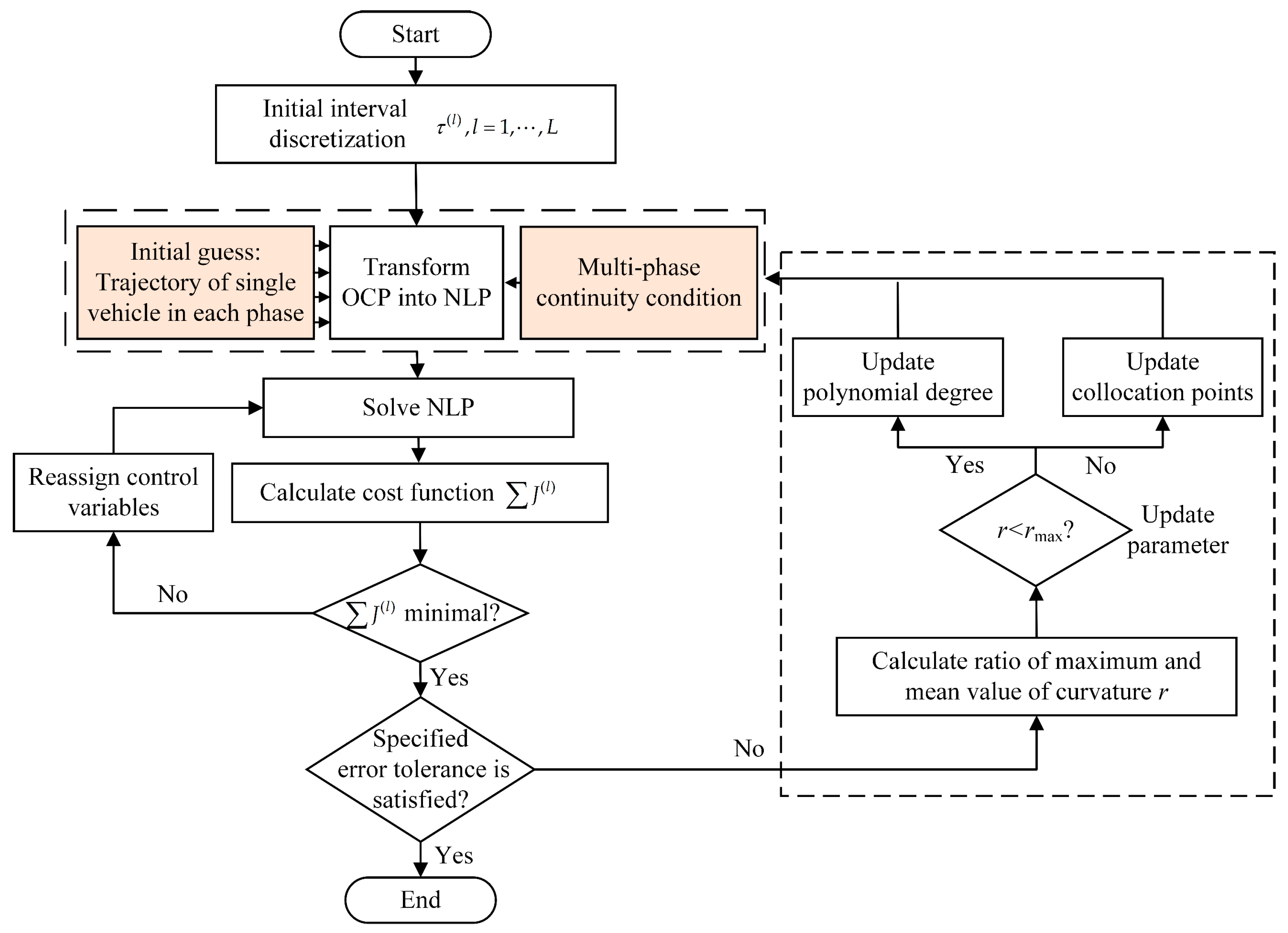
3. The Transformation Process of the Hp-Adaptive Pseudo-Spectral Method

The hp-adaptive pseudo-spectral method has been employed to address the aforementioned Optimal Control Problem (OCP), with the transformation process delineated in Figure 6, which depicts the integration of critical swarm constraints. The spatial–temporal coordination of the initial and final conditions across all phases is enforced as boundary conditions, while inter-vehicle collision avoidance is formulated as a path constraint.

Thrust increment is designated as the control variable. The implementation of these constraints facilitates the construction of the swarm model based on the trajectory optimization of individual Unmanned Aerial Vehicles (UAVs). These constraints are subsequently translated into equality and inequality constraints within a Nonlinear Programming (NLP) framework using the hp-adaptive pseudo-spectral method. This approach initially discretizes the OCP at a set of initial nodes and then automatically refines the distribution of these nodes based on the approximate error in state and control variables, ensuring the precision and convergence of the solution. The output of the planning process comprises a sequence of state and control variables over time, along with the relevant parameters that quantify trajectory performance, including energy consumption and flight distance.

Figure 7 shows the numerical solution procedure of this hp-adaptive pseudo-spectral method in the multi-phase trajectory optimization of fixed-wing swarm [45]. It shows the process of the hp-adaptive pseudo-spectral method employed for the multi-phase trajectory optimization of the swarm. During the transformation of the OCP into the NLP, the trajectory for a single UAV within each phase is computed efficiently, making it suitable as the initial guess for the direct collocation method. The multi-phase continuity condition imposed on the state and control variables across multiple phases are converted into equality constraints at the terminal point of the collocation points.

The direct collocation method demonstrates robustness against initial guesses, allowing the trajectory of a single aircraft in each phase to be used as the initial guess for each member of the swarm. This typical direct collocation method can solve the continuous Bolza form of the OCP by discretizing the multi-phase problem and conveniently transitioning it to a NLP. Ongoing research continues to enhance the performance of the hp-adaptive pseudo-spectral method. Their results indicate that GPM-based planning methods can be effectively integrated into the onboard systems. In the hp-adaptive pseudo-spectral method, the number of discretization points for each phase can be adjusted individually. The basic process of the hp-adaptive pseudo-spectral method includes the discretization of the phase interval, variables, and kinematic model. The following five steps introduce the processes of the multi-phase OCP.

1.

Interval discretization

The trajectory can be summarized as a set of $L$ phases, where $l\in [1,\dots L]$ is a particular phase and ${(\cdot )}^{(l)}$ denotes the variables in the $l$-th phase. In each phase, the time interval is bounded by $[t_0^{(l)},t_f^{(l)}]$.

$${\tau }^{(l)}={\displaystyle \frac{2t^{(l)}-\left(t_f^{(l)}+t_0^{(l)}\right)}{t_f^{(l)}-t_0^{(l)}}}$$

(11)

$$t^{(l)}={\displaystyle \frac{t_f^{(l)}-t_0^{(l)}}{2}}{\tau }^{(l)}+{\displaystyle \frac{t_f^{(l)}+t_0^{(l)}}{2}}$$

(12)

2.

State and control variables discretization

The OCPs are supposed at a finite set of Legendre-Gauss-Radau (LGR) collocation points ${\tau }_m^{(l)}(m=1,2,\dots ,M)$, where $M^{(l)}$ denotes the size of the temporal set [31]. This set includes the zeros of $P_{m-1}^{(l)}(\tau )+P_m^{(l)}(\tau )$, the $M$-th order of the LGR points and ${\tau }_0=-1$. $P_m^{(l)}(\tau )$ is derived from Equation (13).

$$P_m^{(l)}(\tau )={\displaystyle \frac{1}{2^{m}m!}}{\displaystyle \frac{d^m}{d{\tau }^m}}{[{({\tau }^{(l)})}^2-1]}^m$$

(13)

The state variables $X^{(l)}$ are approximated based on $(M+1)$-th Lagrange interpolating polynomials.

$$X^{(l)}(\tau )\approx X_a^{(l)}(\tau )={\displaystyle \sum _{i=0}^M{L}_i^{(l)}}(\tau )X_a^{(l)}({\tau }_i)$$

(14)

where $L_i^{(l)}(\tau )$ are defined as follows:

$$L_i^{(l)}(\tau )={\displaystyle \prod _{j=0,j\ne i}^M\frac{\tau -{\tau }_j}{{\tau }_i-{\tau }_j}}$$

(15)

Additionally, the control variable $U^{(l)}(\tau )$ is approximated based on $M$-th Lagrange interpolating polynomials.

$$U^{(l)}(\tau )\approx U_a^{(l)}(\tau )={\displaystyle \sum _{i=1}^M{L}_i^{*(l)}}(\tau )U_a^{(l)}({\tau }_i)$$

(16)

where $L_i^{*(l)}(\tau )={\displaystyle \prod _{j=1,j\ne i}^M\frac{\tau -{\tau }_j}{{\tau }_i-{\tau }_j}}$.

$L_i^{(l)}(\tau )$ and $L_i^{\ast (l)}(\tau )$ satisfy the Kronecker relation.

$$L_i^{(l)}({\tau }_j)=\left\{\begin{array}{ll}1,\hfill & i=j,\hfill \\ 0,\hfill & i\ne j,\hfill \end{array}\right.$$

(17)

The dynamic constraint is collocated only at the LGR points rather than the boundary points; therefore, additional variables are needed, $X_0^{(l)}=X_a^{(l)}(-1)$. The terminal state $X_a^{(l)}({\tau }_f)$ should be added from the terminal state approximation and Gauss quadrature.

$$X_a^{(l)}({\tau }_f)=X_a^{(l)}({\tau }_0)+{\displaystyle \frac{t_f^{(l)}-t_0^{(l)}}{2}}{\displaystyle \sum _{j=1}^N{w}_j^{(l)}}f(X_a^{(l)}({\tau }_j),U_a^{(l)}({\tau }_j),{\tau }_j;t_0^{(l)},t_f^{(l)})$$

(18)

where $w_j^{(l)}={\displaystyle {\int }_{-1}^1{L}_j^{(l)}}(\tau )\mathrm{d}t$ are the Gauss weights, $j=1,\dots ,M$.

3.

Kinematic model discretization

The expression of the kinematic model can be approximated as follows:

$${\dot{X}}^{(l)}({\tau }_j)\approx {{\dot{X}}_a}^{(l)}({\tau }_j)={\displaystyle \sum _{i=0}^M{\dot{L}}_i^{(l)}}({\tau }_j)X_a^{(l)}({\tau }_i)={\displaystyle \sum _{i=0}^M{D}_{ji}}{X}_a^{(l)}({\tau }_i)j=1,2,\dots ,M$$

(19)

The derivative of each Lagrange polynomial at the LGR points can be represented in a differential approximation matrix $D_{ji}^{(l)}$. The elements of the differential approximation matrix are determined as follows [38]:

$$D_{ji}^{(l)}={\dot{L}}_i^{(l)}({\tau }_j)=\left\{\begin{array}{l}{\displaystyle \frac{{\dot{g}}^{(l)}({\tau }_j)}{({\tau }_j-{\tau }_i){\dot{g}}^{(l)}({\tau }_i)}},(j\ne i)\\ {\displaystyle \frac{{\ddot{g}}^{(l)}({\tau }_j)}{2{\dot{g}}^{(l)}({\tau }_i)}},(j=i)\end{array}\right.j=1,2,\dots ,M$$

(20)

where $g^{(l)}({\tau }_i)=(1+{\tau }_i)[P_M^{(l)}({\tau }_i)-P_{M-1}^{(l)}({\tau }_i)],\hspace{1em}i=0,1,\dots ,M$.

The kinematic model can be transcribed into algebraic constraints via the differential approximation matrix as follows:

$$(F_1^{(l)},F_2^{(l)},\dots ,F_M^{(l)})=0j=1,2,\dots ,M$$

(21)

$$F_j^{(l)}={\displaystyle \sum _{i=0}^M{D}_{ji}^{(l)}}{X}_a^{(l)}({\tau }_i)-{\displaystyle \frac{t_f^{(l)}-t_0^{(l)}}{2}}f(X_a^{(l)}({\tau }_i),U_a^{(l)}({\tau }_j))=0,\hspace{1em}j=1,2,\dots ,M.$$

(22)

4.

Cost function discretization

The general continuous Bolza problem of all phases, expressed by Equation (23), can be approximated by the Gauss quadrature given by Equation (24).

$$J=\min {\displaystyle \sum _{l=1}^L\{\Phi [X(t_0^{(l)}),t_0^{(l)},X(t_f^{(l)}),t_f^{(l)}]+{\displaystyle {\int }_{t_0^{(l)}}^{t_f^{(l)}}g}(X(t),U(t),t)dt}\}$$

(23)

$$J\approx \min {\displaystyle \sum _{l=1}^L[\Phi (X_a^{(l)}({\tau }_0),t_0^{(l)},X_a^{(l)}({\tau }_f),t_f^{(l)})+\frac{t_f^{(l)}-t_0^{(l)}}{2}{\displaystyle \sum _{j=1}^M{\omega }_j^{(l)}}g(X_a^{(l)}({\tau }_j),U_a^{(l)}({\tau }_j),{\tau }_j;t_0^{(l)},t_f^{(l)})]}$$

(24)

5.

Boundary and path constraints discretization

The boundary conditions and path constraints are expressed in the following discretization form:

$$\varphi ({X_a}^{(l)}({\tau }_0),{X_a}^{(l)}({\tau }_M))=0,$$

(25)

$$C(X_a^{(l)}({\tau }_j),U_a^{(l)}({\tau }_j),{\tau }_j;t_0^{(l)},t_f^{(l)})\le 0,\hspace{1em}j=1,2,\dots ,M.$$

(26)

Finally, the original OCP is transformed into an NLP, as detailed in the general form of Equation (27) [46].

$$\begin{gathered} J\approx \min {\displaystyle \sum _{l=1}^L[\Phi (X_a^{(l)}({\tau }_0),t_0^{(l)},X_a^{(l)}({\tau }_f),t_f^{(l)})+\frac{t_f^{(l)}-t_0^{(l)}}{2}{\displaystyle \sum _{j=1}^M{\omega }_j^{(l)}}g(X_a^{(l)}({\tau }_j),U_a^{(l)}({\tau }_j),{\tau }_j;t_0^{(l)},t_f^{(l)})]} \\ \begin{array}{l}s.t.\\ F_j^{(l)}={\displaystyle \sum _{i=0}^M{D}_{ji}^{(l)}}{X}_a^{(l)}({\tau }_i)-{\displaystyle \frac{t_f^{(l)}-t_0^{(l)}}{2}}f(X_a^{(l)}({\tau }_i),U_a^{(l)}({\tau }_j))=0\\ C(X_a^{(l)}({\tau }_j),U_a^{(l)}({\tau }_j),{\tau }_j;t_0^{(l)},t_f^{(l)})\le 0\\ \varphi (X_a^{(l)}({\tau }_0),X_a^{(l)}({\tau }_M))=0,\\ X_a^{(l+1)}({\tau }_0)=X_a^{(l)}({\tau }_M)\\ U_a^{(l+1)}({\tau }_0)=U_a^{(l)}({\tau }_M)\end{array}\begin{array}{l}l=1,2,\dots ,L\\ i=0,1,\dots ,M\\ j=1,2,\dots ,M\end{array} \end{gathered}$$

(27)

The optimization parameters, denoted as $X_a^{(l)}({\tau }_i)$ and $U_a^{(l)}({\tau }_j)$, offer an achievement of reasonable optimality and feasibility tolerances. The Sparse Nonlinear OPTimizer (SNOPT) is used to solves the sparse NLP using variable-order Gaussian quadrature methods, thus accommodating diverse computational demands [47]. To accurately represent the algorithms proposed in the study, based on the descriptions in Figure 6 and the formulas provided, the pseudocode can be structured as follows:

In the pseudocode of Algorithm 1, ${(\cdot )}_{guess}$ is the initial guess of the swarm trajectories based on the optimal result of a single vehicle. ${(\cdot )}_{upper\&lower}$ represents the upper and lower constraints of the variables. ${(\cdot )}_{result}$ represents the output of the algorithm. $\mathsf{\tau }$ is the discretized points vector. $N_{\max }$ is the maximum number of iterations. $K$ represents the kinematic model of the swarm. $\mathsf{\epsilon }$ represents the allowable error vector. $\epsilon$ is the reference error. $\mathcal{R}$ is the differential error, $\mathcal{K}$ is the curvature of the state, and $\mathcal{V}$ is the uniformity of the curvature.

Algorithm 1 Rendezvous Trajectory Planning Process

Input: ${\mathsf{\tau }}_{guess}$, $X_{aguess}$, $U_{aguess}$, $X_{upper\&lower}$, $U_{upper\&lower}$, $n_{\max }$, $D_{safe}$ Output: ${\mathsf{\tau }}_{result}$, $X_{aresult}$, $U_{aresult}$  1: initialize ${\mathsf{\tau }}_{new}={\mathsf{\tau }}_{guess}$, $X_{aref}=X_{aguess}$, $U_{aref}=U_{aguess}$;  2: for $k=1$$\mathrm{to}{N}_{\max }$ do  3:  Calculate $K$, $F$, $J$, $\varphi$, $C$ and form the nonlinear programming $p^{(k)}$;  4:  Solve $p^{(k)}$ to obtain ${X_a}_{opt}^k$ and ${U_a}_{opt}^k$;  5:  Calculate ${\mathsf{\epsilon }}_{iter}$;  6:  if ${\mathsf{\epsilon }}_{iter}\le \mathsf{\epsilon }$ then  7:   $X_{aresult}={X_a}_{opt}^k$, $U_{aresult}={U_a}_{opt}^k$, and ${\mathsf{\tau }}_{result}={\mathsf{\tau }}_{new}$;  8:   break;  9:  else  10:  Calculate $\mathcal{R}$, $\mathcal{K}$, and $\mathcal{V}$;  11:  if $\mathcal{R}>\epsilon$ then  12:  Obtain ${\mathsf{\tau }}_{new}$ by hp-adaptive LGR, ${X_a}_{ref}^{k+1}$, ${U_a}_{ref}^{k+1}$ by interpolate;  13:  end if  14: end if  15: end for

By utilizing thrust increments as virtual control variables, we improved the continuity of the control inputs, reduced the number of adaptive collocation points required in the solution process, and decreased the dimensionality of the Nonlinear Programming (NLP) problem. After the comparison of different results, the number of collocation points for a single trajectory was determined to be 40. The tolerance of the numerical algorithm was set to 10⁻⁵. Compared to the approach without thrust increment virtual control variables, the computation time was significantly reduced from 10 s to 6 s, as measured on an i7-12700k CPU.

4. Simulation and Analysis

In the simulation and analysis section, the effectiveness of the proposed method is validated through two case studies that encompass typical wind energy harvesting trajectory planning. By employing distinct cost functions and constraints to each case, the simulation assesses the robustness and feasibility of the method across different scenarios. The ratio $K_1:K_2:K_3$ reflects the weights of various normalized trajectory costs, enabling the solution of different trajectories. For instance, when $K_1\gg K_2=K_3$, the result is an energy-optimal trajectory, and when $K_2\gg K_1=K_3$, it is a time-optimal trajectory. Considering the normalization of trajectory costs in this study, a parameter combination of 100:1:1 was selected.

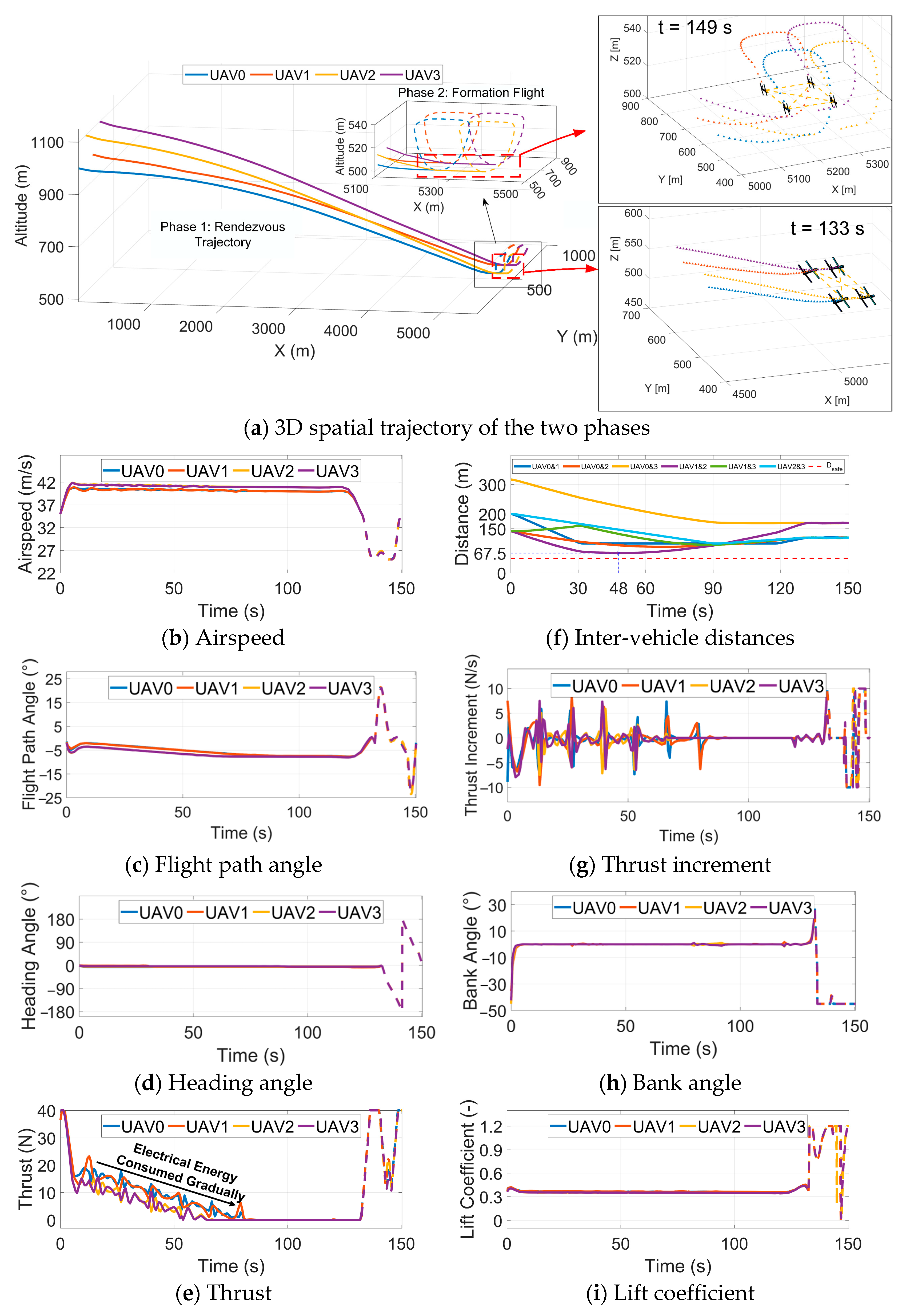
4.1. Low-Altitude Mission Scenario

4.1.1. Optimal Control Model of Low-Altitude Mission

Figure 8 presents the framework of the two-phase OCP in the low-altitude mission scenario. The objective in a low-altitude mission is to maximize the distance for the formation of rendezvous while adhering to a specified electrical energy consumption constraint of 10 Wh (36,000 J) in Phase 1, followed by executing fixed-point surveillance in Phase 2. This case evaluates an air-launch swarm of four members in low-altitude wind conditions. The objective is to plan an open-loop trajectory for the farthest rendezvous formation, constituting Phase 1, followed by a closed-loop trajectory after formation, constituting Phase 2.

The initial and final positions for Phase 1 and 2 of the members are listed in

Table 6. Initial and final state of two-phase trajectory in low-altitude mission.

UAV Identifier	Phase 1		Phase 2
	Initial State (m) $[\mathit{x}({\mathit{t}}_{\mathbf{0}}),\mathit{y}({\mathit{t}}_{\mathbf{0}})\mathbf{,}\mathit{h}({\mathit{t}}_{\mathbf{0}})]$	Final State (m) $[\mathit{x}({\mathit{t}}_{\mathit{f}}^{(\mathbf{1})})\mathbf{,}\mathit{y}({\mathit{t}}_{\mathit{f}}^{(\mathbf{1})})\mathbf{,}\mathit{h}({\mathit{t}}_{\mathit{f}}^{(\mathbf{1})})]$	Final State (m) $[\mathit{x}({\mathit{t}}_{\mathit{f}}^{(\mathbf{2})})\mathbf{,}\mathit{y}({\mathit{t}}_{\mathit{f}}^{(\mathbf{2})})\mathbf{,}\mathit{h}({\mathit{t}}_{\mathit{f}}^{(\mathbf{2})})]$
UAV 0	[0, 0, 1000]	[x0(tf(1)), y0(tf(1)), 500]	[x0(tf(2)), y0(tf(2)), 500]
UAV 1	[0, 200, 1000]	[x0(tf(1)), y0(tf(1)) + 120, 500]	[x0(tf(2)), y0(tf(2)) + 120, 500]
UAV 2	[0, 100, 1100]	[x0(tf(1)) + 120, y0(tf(1)), 500]	[x0(tf(2)) + 120, y0(tf(2)), 500]
UAV 3	[0, 300, 1100]	[x0(tf(1)) + 120, y0(tf(1)) + 120, 500]	[x0(tf(2)) + 120, y0(tf(2)) + 120, 500]

. The remaining state variables, which include $[V_a(t_0),\gamma (t_0),\psi (t_0),T(t_0)]$, are $[35,\mathrm{free},\mathrm{free},\mathrm{free}]$, which are the same in all initial and final states. Two UAVs start at an altitude of 1.1 km and the other two at 1 km, with a horizontal separation of 200 m between the UAVs at the same altitude. For Phase 1, the final rendezvous altitude is set at 500 m. Subsequently, the UAVs form a 120 m rectangular formation and transition into a close-loop loiter trajectory for Phase 2. The linear wind model is oriented along the positive direction of the X-axis.

4.1.2. Swarm Trajectory of Low-Altitude Mission

Figure 9 shows the trajectory planning without the consideration of the wind effect, while Figure 10 includes the effect of the wind. Each set of figures presents a sequence that includes the three-dimensional (3D) spatial trajectory, airspeed, flight path angle, heading angle, thrust, inter-vehicle distances, thrust increments, bank angle, and lift coefficient.

Comparing Figure 9a and Figure 10a reveals that irrespective of wind consideration, the trajectories show all UAVs successfully reaching the designated altitude and completing formation rendezvous simultaneously. Both trajectories in Phase 2 exhibit typical closed-loop wind energy harvesting trajectories. Under the constraint of 10 Wh electrical energy consumption and a 500 m relative altitude in Phase 1, the trajectory planned with wind effect consideration achieves a distance of 9467 m compared to 5284 m for the planning without wind energy, representing a 79% increase. Comparing the state and control variables in the subplots under wind conditions, Phase 1 lasts 185 s, and Phase 2 lasts 26 s. Without wind consideration, Phase 1 lasts 133 s, and Phase 2 lasts 17 s. Additionally, the state and control variables exhibit a continuity between the endpoint of Phase 1 and the initial of Phase 2, satisfying all constraints.

The ‘f’ subplot of Figure 9 and Figure 10 illustrates the changes in distances between swarm members. The minimum distances between the UAVs are recorded as 67.5 m and 79 m, respectively, satisfying the safety distance constraint. During Phase 2, the inter-vehicle distances remain stable with minimal fluctuation, indicating an excellent spatial–temporal consistency in the formation flight.

In trajectories incorporating wind energy harvesting, there is an initiation stage in Phase 1 where UAVs consume their electrical energy to ascend and accumulate potential energy. This strategy positions them at higher altitudes where the wind speed magnitude is greater, facilitating a prolonged leeward descent that is advantageous for harvesting wind energy and covering a greater distance.

Figure 11a,b illustrate the potential, kinetic, and electrical energy of the results with and without wind energy consideration. The specific parameters are listed in

Table 7. Comparison of trajectory parameters with different time and energy weights.

	Wind Condition	Maximum Rendezvous Distance (m)	Phase Duration (s)	Maximum Electrical Energy Consumption (Wh)	Maximum Average Power (W)	Percentage of Average Power	Percentage of Expand Range
Phase 1: Rendezvous Trajectory	No-wind	5284	133	10	270.7	100%	100%
	Tailwind	9467	185	10	194.6	71.9%	179.2%
Phase 2: Formation Flight	No-wind	N/A	17	3.9	825.9	100%	N/A
	Tailwind	N/A	26	5	692.3	83.8%	N/A

, the closed-loop trajectories consume 3.9 Wh and 5.0 Wh per cycle, with a cycle time of 17.8 s and 25.6 s in Phase 2. Their electrical energy consumption rate is 0.22 Wh/s and 0.19 Wh/s. That means the endurance of a fixed-point close-loop flight would increase by up to 16%. During the descent rendezvous phase, kinetic energy remains stable regardless of wind energy consideration. However, both the potential and electrical energy show a smoother decline when the wind energy is utilized, indicating that the energy difference along the trajectory is supplemented by the wind. All results show that the proposed method effectively addresses the multi-phase wind energy harvesting trajectory planning.

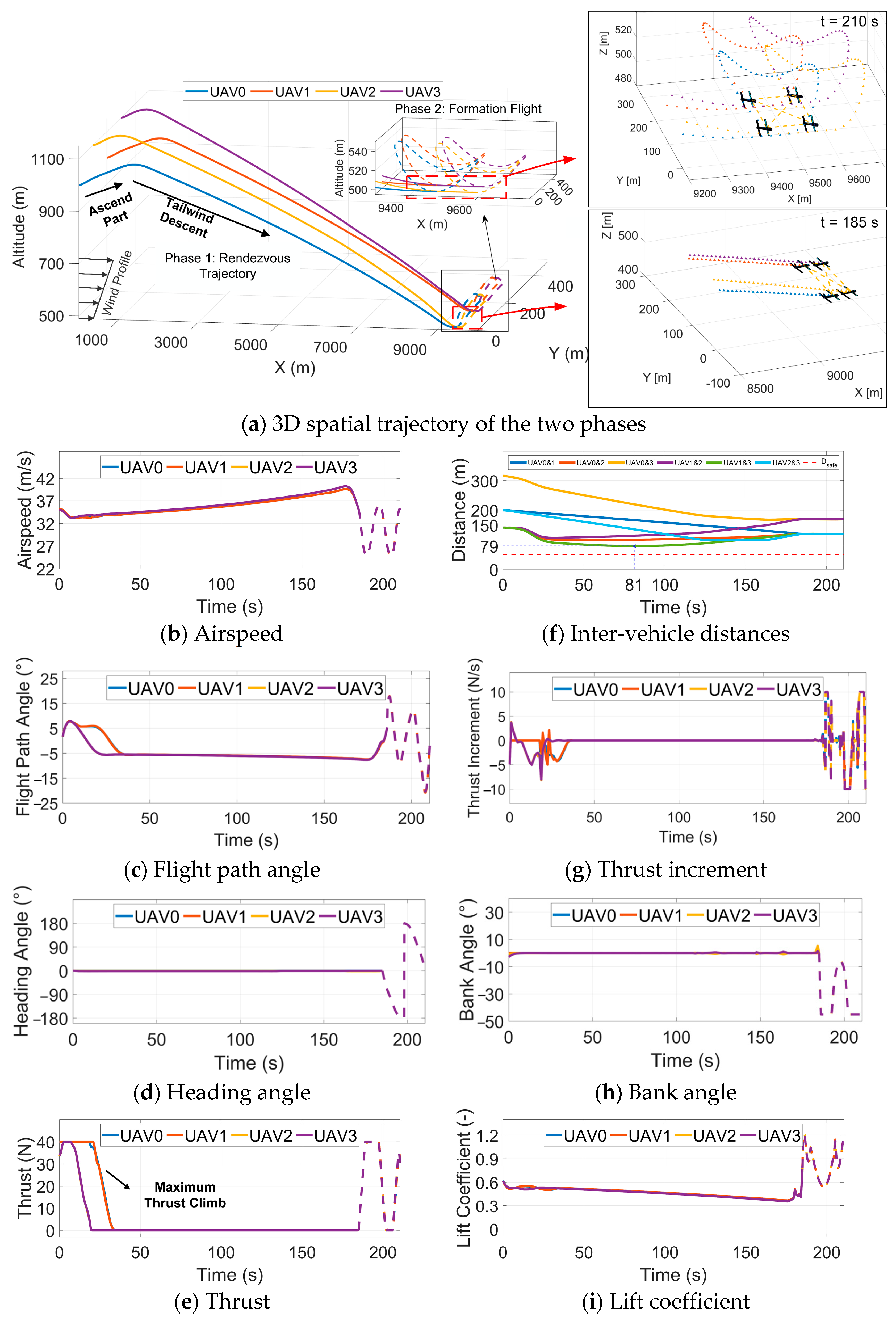
4.2. High-Altitude Mission Scenario

4.2.1. Optimal Control Model of High-Altitude Mission

Figure 12 presents the framework of the two-phase OCP in the high-altitude mission scenario. The objective function for the high-altitude mission aims to minimize the electrical energy consumption required to reach a specified position for formation rendezvous (Phase 1), followed by an open-loop crosswind forward flight (Phase 2). This case focuses on optimizing the energy rendezvous trajectory to a designed endpoint with a subsequent forward tracking in crosswind conditions. Here, the goal is to plan an open-loop trajectory to balance electrical energy consumption and time, constituting Phase 1, followed by another open-loop trajectory for forward tracking after formation in Phase 2.

The initial and final positions for Phase 1 and 2 of the four members are listed in

Table 8. The initial and final state of the two-phase trajectory in a high-altitude mission.

UAV Identifier	Phase 1		Phase 2
	Initial State (m) $[\mathit{x}({\mathit{t}}_{\mathbf{0}})\mathbf{,}\mathit{y}({\mathit{t}}_{\mathbf{0}})\mathbf{,}\mathit{h}({\mathit{t}}_{\mathbf{0}})]$	Final State (m) $[\mathit{x}({\mathit{t}}_{\mathit{f}}^{(\mathbf{1})})\mathbf{,}\mathit{y}({\mathit{t}}_{\mathit{f}}^{(\mathbf{1})})\mathbf{,}\mathit{h}({\mathit{t}}_{\mathit{f}}^{(\mathbf{1})})]$	Final State (m) $[\mathit{x}({\mathit{t}}_{\mathit{f}}^{(\mathbf{2})})\mathbf{,}\mathit{y}({\mathit{t}}_{\mathit{f}}^{(\mathbf{2})})\mathbf{,}\mathit{h}({\mathit{t}}_{\mathit{f}}^{(\mathbf{2})})]$
UAV 0	[0, 0, 8000]	[20,000, 20,000, 6000]	[22,000, 22,000, 6000]
UAV 1	[0, 200, 8000]	[20,000, 20,120, 6000]	[22,000, 22,120, 6000]
UAV 2	[0, 100, 8200]	[20,120, 20,000, 6000]	[22,120, 22,000, 6000]
UAV 3	[0, 300, 8200]	[20,120, 20,120, 6000]	[22,120, 22,120, 6000]

. The remaining state variables, which include $[V_a(t_0),\gamma (t_0),\psi (t_0),T(t_0)]$, are $[35,\mathrm{free},\mathrm{free},\mathrm{free}]$, which are the same in all initial and final states. Two UAVs are deployed at an altitude of 8.2 km while the other two start at 8 km, with a horizontal separation of 200 m between UAVs at the same altitude. The rendezvous trajectory terminates at an altitude of 6 km where they form a 120 m rectangular formation, marking the endpoint of Phase 1. Then, the UAV formation transitions to an open-loop tracking trajectory in Phase 2. The linear wind gradient is oriented along the positive X-axis direction.

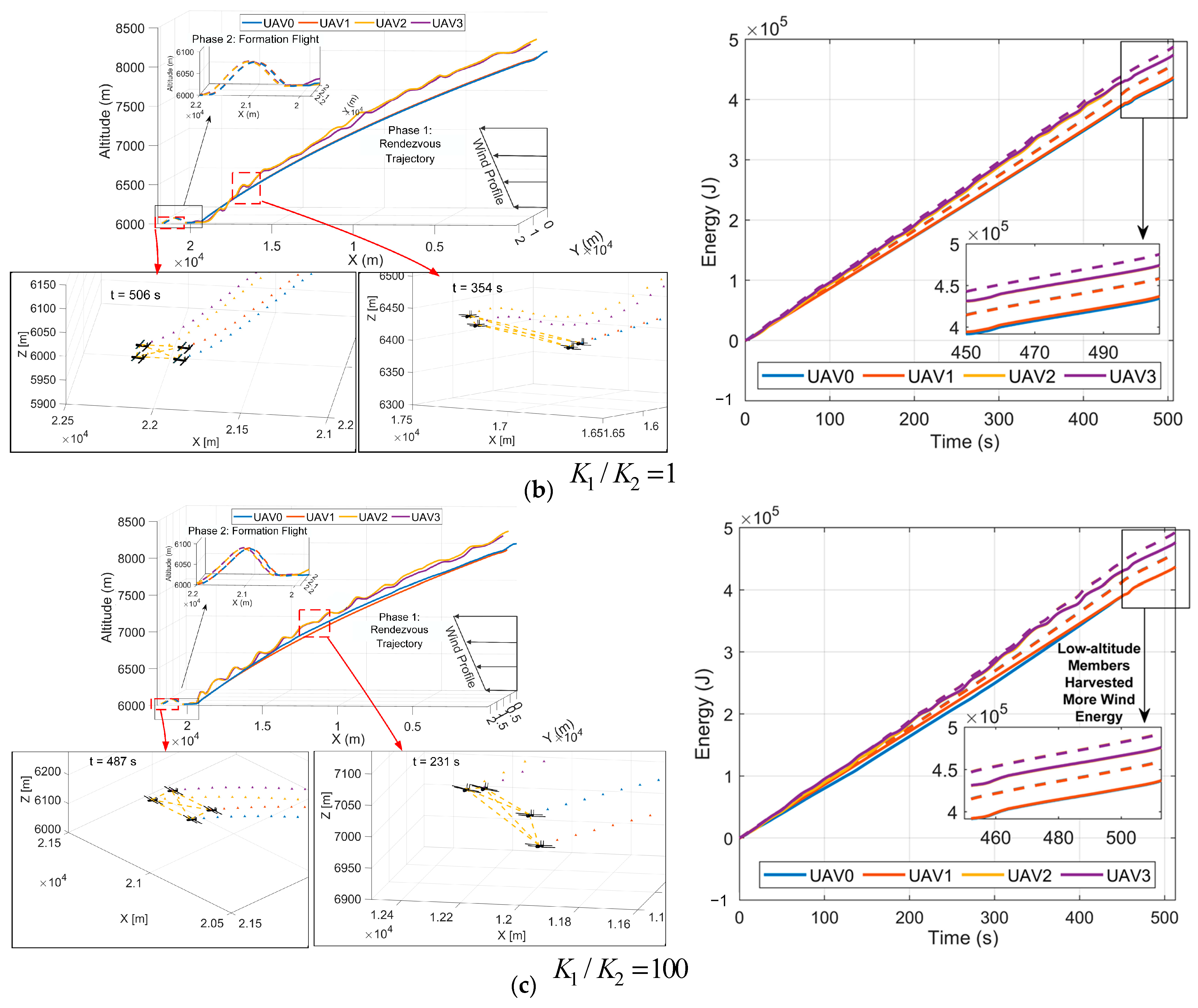
4.2.2. Swarm Trajectory of High-Altitude Mission

Figure 13 illustrates the results of the rendezvous trajectories for a four-UAV air-launch swarm operating at high altitudes, employing a cost function with varying weight on energy and time. The figure includes subplots of three-dimensional trajectories and their energy changes, demonstrating how adjustments to the weight in the cost function influence both the energy efficiency and phase duration. The three-dimensional trajectory plots, incorporating five different cost functions with adjustments to the energy weight $K_1/K_2$ from 0.01 to 100 while keeping time and position weights, reveal that the results emphasize different weights on time and energy can be computed successfully. Four UAVs simultaneously reach the endpoint altitude to complete the formation rendezvous, and the formation shape is maintained for a crosswind open-loop forward track in Phase 2. When the endpoint formation position for Phase 1 is fixed, these trajectories indicate that the optimal energy consumption is 0, with a corresponding flight time of 452 s. In contrast, the maximum energy consumption is about 18 Wh, corresponding to a trajectory time of 402 s. This represents a 12.5% increase in time compared to the trajectory with minimal energy consumption. This underscores the critical consideration of time-sensitive decisions in swarm mission planning. The UAVs effectively utilize the wind energy as a kinetic energy supplement in trajectories with a much lower electrical consumption. The state and control variables of the five results satisfy their respective constraints, and the variables’ transition from Phase 1 to Phase 2 maintains continuity.

During Phase 2, the inter-vehicle distances within the formation are stable, indicating strong spatial and temporal consistency in the formation flight. In a trajectory prioritizing time, more electrical and wind energy are utilized to supplement kinetic energy, resulting in minimal spatial fluctuation and shorter trajectory lengths. Conversely, in trajectory prioritizing energy consumption, the two UAVs with higher potential energy frequently employ climbing and diving maneuvers to consume wind and potential energy. A comparison of trajectory parameters with different time and energy weights is shown in

Table 9. Comparison of trajectory parameters with different time and energy weights.

	${\mathit{K}}_{\mathbf{1}}\mathbf{/}{\mathit{K}}_{\mathbf{2}}$	Phase Duration (s)	Maximum Electrical Energy Consumption (Wh)	Maximum Average Power (W)	Percentage of Average Power
Phase 1: Rendezvous Trajectory	0.01	402	18	161.2 W	100%
	0.1	439	3	24.6 W	15.3%
	1	449	0.1	0.8 W	0.5%
	10	451	0	0	0
	100	452	0	0	0
Phase 2: Formation Flight	0.01	49.7	15	1086.5 W	100%
	0.1	50	14.7	1058.4 W	97.4%
	1	57	12	757.9 W	69.8%
	10	60	11.9	714 W	65.7%
	100	61	11.8	696.4 W	64.1%

. It contrasts with traditional dynamic soaring, which involves turning maneuvers for energy consumption. The electrical energy consumption rate during Phase 2 of the five results ranges from 0.3 to 0.19 Wh/s. When advancing in a crosswind, the effective utilization of wind energy can extend the endurance by 58%, markedly enhancing capability for tracking applications.

Compared to the farthest rendezvous formation position in the low altitude mission, the state and control variables in the high-altitude mission exhibit more significant fluctuations. The adoption of thrust increment input helps mitigate severe fluctuations in thrust input, thus enhancing the traceability of the planning results. The proposed method effectively addresses trajectory planning problems across various weights in cost function terms.

5. Conclusions

This paper proposes a multi-phase wind energy harvesting trajectory planning method for the rendezvous and formation flight of air-launched UAV swarms deployed from different mother planes at various initial positions. This research focuses on air-launched, fixed-wing swarm systems and explores multi-phase wind energy harvesting trajectories with integrated spatial–temporal coordination, effectively extending wind energy harvesting strategies from single UAVs to the swarm level. Unlike previous studies that might focus on simpler kinematic models or single UAV scenarios, this paper integrates continuous constraints on multi-phase trajectories and incorporates a comprehensive kinematic model based on 3DOF for each UAV. The hp-adaptive pseudo-spectral method is introduced for the discretization and transformation of the OCP into an NLP problem. The main conclusions are as follows:

(1)

Harvesting wind energy can significantly enhance the endurance and range of air-launched swarm rendezvous and formation flight. Under favorable wind conditions, the farthest formation distance of the swarm can expand by over 50% under the same electrical energy consumption constraints, substantially reducing the average power required for the rendezvous trajectory. The range extension of air-launched swarms is significantly influenced by the duration constraints when employing wind energy harvesting strategies. The flexibility to adjust the cost function weights based on the specific requirements of a mission and its environment ensures the optimal deployment and utilization of the air-launch UAV swarms in wind conditions.

(2)

Utilizing thrust as a state variable and thrust increment as a control variable enhances the continuity of thrust inputs and guarantees the feasibility of trajectory planning. All trajectories satisfy the constraints of the variables, boundary conditions, paths, and multi-phase connections. Simulation results demonstrate significant energy savings in both low- and high-altitude mission scenarios. Efficient wind energy utilization can double the maximum formation rendezvous distance and even allow for rendezvous without electrical power consumption when the phase durations are extended reasonably. The subsequent formation flight phase exhibits a maximum endurance increase of 58%.

(3)

This paper explores a more comprehensive utilization of the potential, kinetic, electrical, and wind energies for the rendezvous and formation missions of UAV swarms. By optimizing trajectory planning for swarm rendezvous and formation flight, this approach significantly reduces electrical energy consumption during these critical phases of the mission. This reduction in energy use directly contributes to extending the range and endurance of the UAVs, thereby enhancing the operational capabilities of the swarm in subsequent mission phases.

Future work could incorporate a rolling horizon OCP to reveal the impact of time and spatial variations in wind conditions. More accurate wind field modeling methods are also worth studying. The efficiency and convergence of the direct collocation method still need improvement, which can be achieved by transforming swarm constraints into soft constraints through their implementation in the cost functions.

References

1. Sheng, H.; Zhang, J.; Yan, Z.; Yin, B.; Liu, S.; Bai, T.; Wang, D. New Multi-UAV Formation Keeping Method Based on Improved Artificial Potential Field. Chin. J. Aeronaut. 2023, 36, 249–270. [Google Scholar] [CrossRef]
2. Han, T.; Tang, A.; Zhou, H.; Xu, D.; Xie, L. Multiple UAV Cooperative Path Planning Based on LASSA Method. Syst. Eng. Electron. 2022, 44, 233–241. [Google Scholar] [CrossRef]
3. Liang, H.J.; Cui, T.; Ma, J.J. Research on the Development Status and Trend of Typical Unmanned Air Attack Weapon. Ship Electron. Eng. 2021, 41, 9–13. [Google Scholar]
4. Lu, Y.F.; Chen, Q.Y.; Wang, P.; Wang, B.; Guo, Z. Design and Experiment of a Small Air-Launched UAV. Acta Aeronaut. Astronaut. Sin. 2023, 44, 322–332. [Google Scholar] [CrossRef]
5. Fu, X.; Cui, H.; Gao, X. Distributed Solving Method of Multi-UAV Rendezvous Problem. Syst. Eng. Electron. 2015, 37, 1797–1802. [Google Scholar]
6. Cheng, Z.; Zhao, L.; Shi, Z. Decentralized Multi-UAV Path Planning Based on Two-Layer Coordinative Framework for Formation Rendezvous. IEEE Access 2022, 10, 45695–45708. [Google Scholar] [CrossRef]
7. Chang, J.; Laliberté, J. Trajectory Optimization for Dynamic Soaring Remotely Piloted Aircraft with Under-Wing Solar Panels. J. Aircr. 2023, 60, 581–588. [Google Scholar] [CrossRef]
8. Kempton, J.A.; Wynn, J.; Bond, S.; Evry, J.; Fayet, A.L.; Gillies, N.; Guilford, T.; Kavelaars, M.; Juarez-Martinez, I.; Padget, O.; et al. Optimization of Dynamic Soaring in a Flap-Gliding Seabird Affects Its Large-Scale Distribution at Sea. Sci. Adv. 2022, 8, eabo0200. [Google Scholar] [CrossRef]
9. Sachs, G.; Grüter, B. Trajectory Optimization and Analytic Solutions for High-Speed Dynamic Soaring. Aerospace 2020, 7, 47. [Google Scholar] [CrossRef]
10. Idrac, P. Experimental Study of the “Soaring” of Albatrosses. Nature 1925, 115, 532. [Google Scholar] [CrossRef]
11. Hong, H.; Grüter, B.; Piprek, P.; Holzapfel, F. Smooth Free-Cycle Dynamic Soaring in Unspecified Shear Wind via Quadratic Programming. Chin. J. Aeronaut. 2022, 35, 19–29. [Google Scholar] [CrossRef]
12. Sachs, G.; Traugott, J.; Nesterova, A.P.; Dell’Omo, G.; Kümmeth, F.; Heidrich, W.; Vyssotski, A.L.; Bonadonna, F. Flying at No Mechanical Energy Cost: Disclosing the Secret of Wandering Albatrosses. PLoS ONE 2012, 7, e41449. [Google Scholar] [CrossRef] [PubMed]
13. Bencatel, R.; Kabamba, P.; Girard, A. Perpetual Dynamic Soaring in Linear Wind Shear. J. Guid. Control Dyn. 2014, 37, 1712–1716. [Google Scholar] [CrossRef]
14. Wang, W.; An, W.; Song, B. Modeling and Application of Dynamic Soaring by Unmanned Aerial Vehicle. Appl. Sci. 2022, 12, 5411. [Google Scholar] [CrossRef]
15. Mir, I.; Maqsood, A.; Eisa, S.A.; Taha, H.; Akhtar, S. Optimal Morphing—Augmented Dynamic Soaring Maneuvers for Unmanned Air Vehicle Capable of Span and Sweep Morphologies. Aerosp. Sci. Technol. 2018, 79, 17–36. [Google Scholar] [CrossRef]
16. Wang, W.; An, W.; Song, B. Dynamic Soaring Parameters Influence Regularity Analysis on UAV and Soaring Strategy Design. Drones 2023, 7, 271. [Google Scholar] [CrossRef]
17. Fan, W.; Liu, Y.; Chappell, A.; Dong, L.; Xu, R.; Ekström, M.; Fu, T.-M.; Zeng, Z. Evaluation of Global Reanalysis Land Surface Wind Speed Trends to Support Wind Energy Development Using in Situ Observations. J. Appl. Meteorol. Climatol. 2021, 60, 33–50. [Google Scholar] [CrossRef]
18. Deittert, M.; Richards, A.; Toomer, C.A.; Pipe, A. Engineless Unmanned Aerial Vehicle Propulsion by Dynamic Soaring. J. Guid. Control Dyn. 2009, 32, 1446–1457. [Google Scholar] [CrossRef]
19. Sachs, G.; Grüter, B. Optimization of Thrust-Augmented Dynamic Soaring. J. Optim. Theory Appl. 2022, 192, 960–978. [Google Scholar] [CrossRef]
20. Zhao, Y.J.; Qi, Y.C. Minimum Fuel Powered Dynamic Soaring of Unmanned Aerial Vehicles Utilizing Wind Gradients. Optim. Control. Appl. Methods 2004, 25, 211–233. [Google Scholar] [CrossRef]
21. Zhao, Y.; Zheng, Z.; Liu, Y. Survey on Computational-Intelligence-Based UAV Path Planning. Knowl.-Based Syst. 2018, 158, 54–64. [Google Scholar] [CrossRef]
22. Liu, Y.; Chen, C.; Wang, Y.; Zhang, T.; Gong, Y. A Fast Formation Obstacle Avoidance Algorithm for Clustered UAVs Based on Artificial Potential Field. Aerosp. Sci. Technol. 2024, 147, 108974. [Google Scholar] [CrossRef]
23. Li, X.; Wang, L.; Wang, H.; Tao, L.; Wang, X. A Warm-Started Trajectory Planner for Fixed-Wing Unmanned Aerial Vehicle Formation. Appl. Math. Model. 2023, 122, 200–219. [Google Scholar] [CrossRef]
24. Xie, J.; Carrillo, L.R.G.; Jin, L. Path Planning for UAV to Cover Multiple Separated Convex Polygonal Regions. IEEE Access 2020, 8, 51770–51785. [Google Scholar] [CrossRef]
25. Li, Z.; Langelaan, J.W. Parameterized Trajectory Planning for Dynamic Soaring. In Proceedings of the AIAA Scitech 2020 Forum, Orlando, FL, USA, 6–10 January 2020; American Institute of Aeronautics and Astronautics: Reston, VA, USA, 2020. [Google Scholar]
26. Zhao, J.S.; Shang, T.; Zhang, J.M.; Cheng, X.M.; Liu, J.L. Pseudo-Spectral Trajectory Optimization Method with Constraint on the Change Rate of Control Variables. J. Astronaut. 2022, 43, 1368–1377. [Google Scholar]
27. Teng, J.; An, Y.; Wang, L. Time-Optimal Control Problem for a Linear Parameter Varying System with Nonlinear Item. J. Frankl. Inst. 2022, 359, 859–869. [Google Scholar] [CrossRef]
28. Chai, R.; Tsourdos, A.; Savvaris, A.; Xia, Y.; Chai, S. Real-Time Reentry Trajectory Planning of Hypersonic Vehicles: A Two-Step Strategy Incorporating Fuzzy Multiobjective Transcription and Deep Neural Network. IEEE Trans. Ind. Electron. 2019, 67, 6904–6915. [Google Scholar] [CrossRef]
29. Egerstedt, M.; Martin, C.F. Optimal Trajectory Planning and Smoothing Splines. Automatica 2001, 37, 1057–1064. [Google Scholar] [CrossRef]
30. Liu, G.; Li, B.; Ji, Y. A Modified HP-Adaptive Pseudospectral Method for Multi-UAV Formation Reconfiguration. ISA Trans. 2022, 129, 217–229. [Google Scholar] [CrossRef]
31. Lu, Y.; Hu, J.; Chen, G.; Liu, A.; Feng, J. Optimization of Water-Entry and Water-Exit Maneuver Trajectory for Morphing Unmanned Aerial-Underwater Vehicle. Ocean. Eng. 2022, 261, 112015. [Google Scholar] [CrossRef]
32. Flanzer, T.; Bower, G.; Kroo, I. Robust Trajectory Optimization for Dynamic Soaring. In Proceedings of the AIAA Guidance, Navigation, and Control Conference, Minneapolis, MN, USA, 13–16 August 2012; p. 4603. [Google Scholar]
33. Zhao, Y.J. Optimal Patterns of Glider Dynamic Soaring. Optim. Control Appl. Meth. 2004, 25, 67–89. [Google Scholar] [CrossRef]
34. Zhang, T.; Su, H.; Gong, C. Hp-Adaptive RPD Based Sequential Convex Programming for Reentry Trajectory Optimization. Aerosp. Sci. Technol. 2022, 130, 107887. [Google Scholar] [CrossRef]
35. Park, J.; Kim, I.; Suk, J.; Kim, S. Trajectory Optimization for Takeoff and Landing Phase of UAM Considering Energy and Safety. Aerosp. Sci. Technol. 2023, 140, 108489. [Google Scholar] [CrossRef]
36. Wang, Z. Optimal Trajectories and Normal Load Analysis of Hypersonic Glide Vehicles via Convex Optimization. Aerosp. Sci. Technol. 2019, 87, 357–368. [Google Scholar] [CrossRef]
37. Luo, S.; Sun, Q.; Tao, J.; Liang, W.; Chen, Z. Trajectory Planning and Gathering for Multiple Parafoil Systems Based on Pseudo-Spectral Method. In Proceedings of the 2016 35th Chinese Control Conference (CCC), Chengdu, China, 27–29 July 2016; IEEE: Piscataway, NJ, USA, 2016; pp. 2553–2558. [Google Scholar]
38. Gao, X.Z.; Hou, Z.X.; Guo, Z.; Chen, X.Q.; Chen, X.Q. Joint Optimization of Battery Mass and Flight Trajectory for High-Altitude Solar-Powered Aircraft. Proc. Inst. Mech. Eng. Part G J. Aerosp. Eng. 2014, 228, 2439–2451. [Google Scholar] [CrossRef]
39. Sachs, G.; Da Costa, O. Dynamic Soaring in Altitude Region below Jet Streams. In Proceedings of the AIAA Guidance, Navigation, and Control Conference and Exhibit, Keystone, CO, USA, 21–24 August 2006; American Institute of Aeronautics and Astronautics: Reston, VA, USA, 2006. [Google Scholar]
40. Liu, D.N. Research on Mechanism and Trajectory Optimization for Dynamic Soaring with Fixed-Wing Unmanned Aerial Vehicles. Ph.D. Thesis, Graduate School of National University of Defense Technology, Changsha, China, 2016. [Google Scholar]
41. Gao, X.-Z.; Hou, Z.-X.; Guo, Z.; Fan, R.-F.; Chen, X.-Q. Analysis and Design of Guidance-Strategy for Dynamic Soaring with UAVs. Control Eng. Pract. 2014, 32, 218–226. [Google Scholar] [CrossRef]
42. Guo, W.; Zhao, Y.J.; Capozzi, B. Optimal Unmanned Aerial Vehicle Flights for Seeability and Endurance in Winds. J. Aircr. 2011, 48, 305–314. [Google Scholar] [CrossRef]
43. Mir, I.; Eisa, S.A.; Maqsood, A. Review of Dynamic Soaring: Technical Aspects, Nonlinear Modeling Perspectives and Future Directions. Nonlinear Dyn. 2018, 94, 3117–3144. [Google Scholar] [CrossRef]
44. Shaw-Cortez, W.E.; Frew, E. Efficient Trajectory Development for Small Unmanned Aircraft Dynamic Soaring Applications. J. Guid. Control Dyn. 2015, 38, 519–523. [Google Scholar] [CrossRef]
45. Xiao, Z.; Wang, Q.; Sun, P.; You, B.; Feng, X. Modeling and Energy-Optimal Control for High-Speed Trains. IEEE Trans. Transp. Electrif. 2020, 6, 797–807. [Google Scholar] [CrossRef]
46. Kelly, M. An Introduction to Trajectory Optimization: How to Do Your Own Direct Collocation. SIAM Rev. 2017, 59, 849–904. [Google Scholar] [CrossRef]
47. Betts, J.T.; Huffman, W.P. Application of Sparse Nonlinear Programming to Trajectory Optimization. J. Guid. Control Dyn. 1992, 15, 198–206. [Google Scholar] [CrossRef]
Figure 1. Diagram illustrating the optimal two-phase wind energy harvesting trajectory of air-launched UAV swarms from different mother planes.
Drones 08 00709 g001
Figure 2. Typical wind profile of the altitude range [39].
Drones 08 00709 g002
Figure 3. Three views and an axonometric view of the air-launched UAV.
Drones 08 00709 g003
Figure 4. Aerodynamic and thrust forces acting on the UAV and the aerodynamic angles.
Drones 08 00709 g004
Figure 5. Joint wind energy harvesting trajectories of fixed-wing swarms. (a) Closed-loop trajectories in loiter mode; (b) Open-loop trajectories for rendezvous.
Drones 08 00709 g005
Figure 6. Transformation process of the multi-phase trajectory OCP for air-launched swarms in the hp-adaptive pseudo-spectral method, l [ 1 , L ] is the phase number.
Drones 08 00709 g006
Figure 7. The numerical solution procedure of the hp-adaptive pseudo-spectral method in the multi-phase trajectory optimization of fixed-wing swarm, l [ 1 , L ] is the phase number.
Drones 08 00709 g007
Figure 8. Framework of two-phase OCP in the low-altitude mission scenario.
Drones 08 00709 g008
Figure 9. Trajectory for the low-altitude mission scenarios without wind energy harvesting in an altitude range of 1.1–0.5 km.
Drones 08 00709 g009
Figure 10. Trajectory for the low-altitude mission scenarios with wind energy harvesting in an altitude range of 1.1–0.5 km.
Drones 08 00709 g010
Figure 11. The potential, electrical, and kinetic energy in the low-altitude mission scenario.
Drones 08 00709 g011
Figure 12. Framework of two-phase OCP in the high-altitude mission scenario.
Drones 08 00709 g012
Figure 13. Three-dimensional spatial trajectory and energy diagram of the five cost functions in a high-altitude mission in an altitude range of 8.3–6 km.
Drones 08 00709 g013aDrones 08 00709 g013b