
A Unified Collision Avoidance Trajectory Planning with Dual Variables for Collaborative Aerial Transportation Systems


Abstract
1. Introduction
- Unlike previous research on trajectory planning for collaborative transportation systems in open environments [19,20,21,22], this study focuses on developing methods for obstacle avoidance in collaborative transportation systems operating in complex, obstacle-filled environments, aiming to enhance safety in challenging scenarios. Although some studies [23,24] have addressed trajectory planning in such environments, they did not consider transportation time as a critical factor. Additionally, the approach in [23] lacked scalability for systems with different numbers of UAVs. To bridge these gaps, this paper presents a unified obstacle avoidance trajectory planning method that integrates transportation time as a key objective and is designed for systems with two or more UAVs. Real-world experiments are conducted on a self-built collaborative transportation platform to assess the effectiveness and scalability of the proposed method across systems with varying numbers of UAVs.
- In the trajectory planning problem for the transportation system, system dynamics, actuation, safety, and formation constraints are taken into account to obtain the quick delivery trajectory for reaching the target point. The resulting optimization problem, formed by these constraints, is inherently non-convex, thus imposing a significant computational burden. To accelerate the solution of the optimization problem, the collision avoidance constraints are established using dual variables.
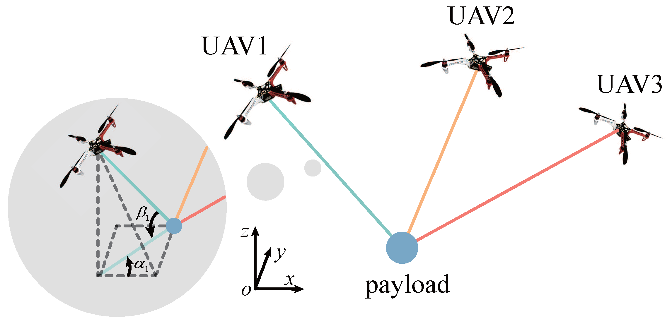
2. Dynamic Model of the Collaborative Aerial Transportation System
3. Discrete Trajectory Optimization Problem Formulation
- (1)
- Dynamics constraint
- (2)
- Actuation constraint
- (3)
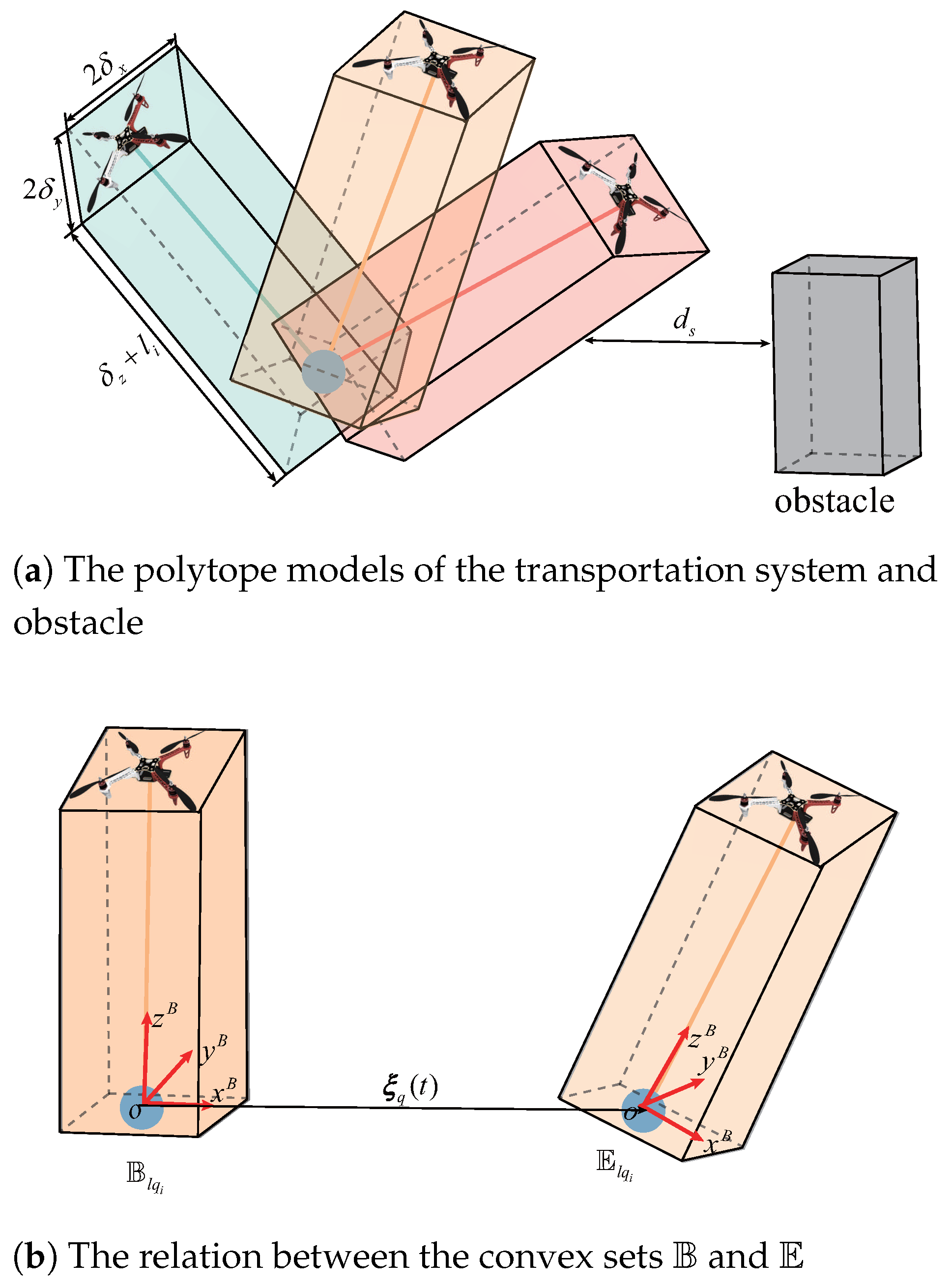
- Safety constraint
- (4)
- Formation constraint
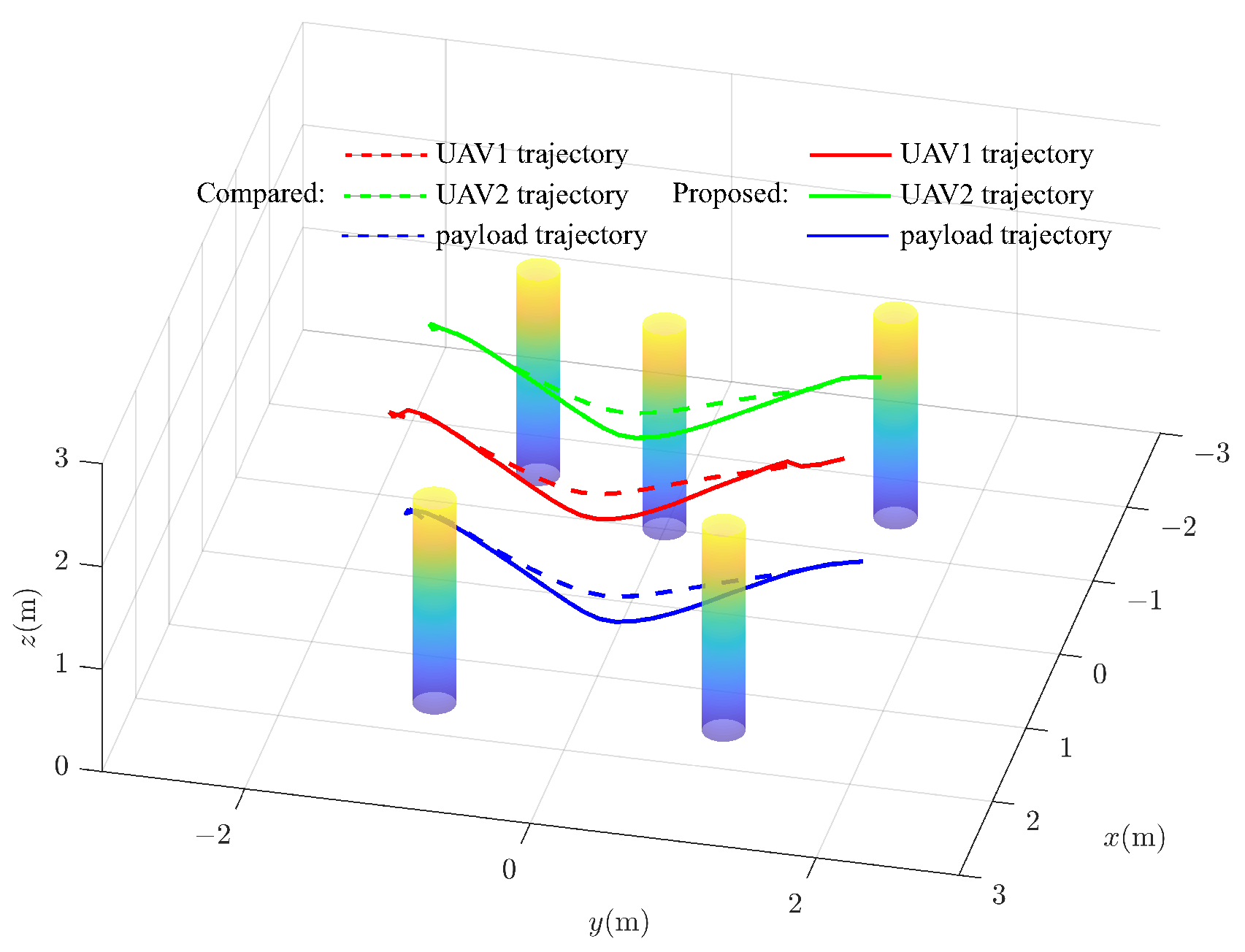
4. Simulation and Experimental Results
4.1. Simulation
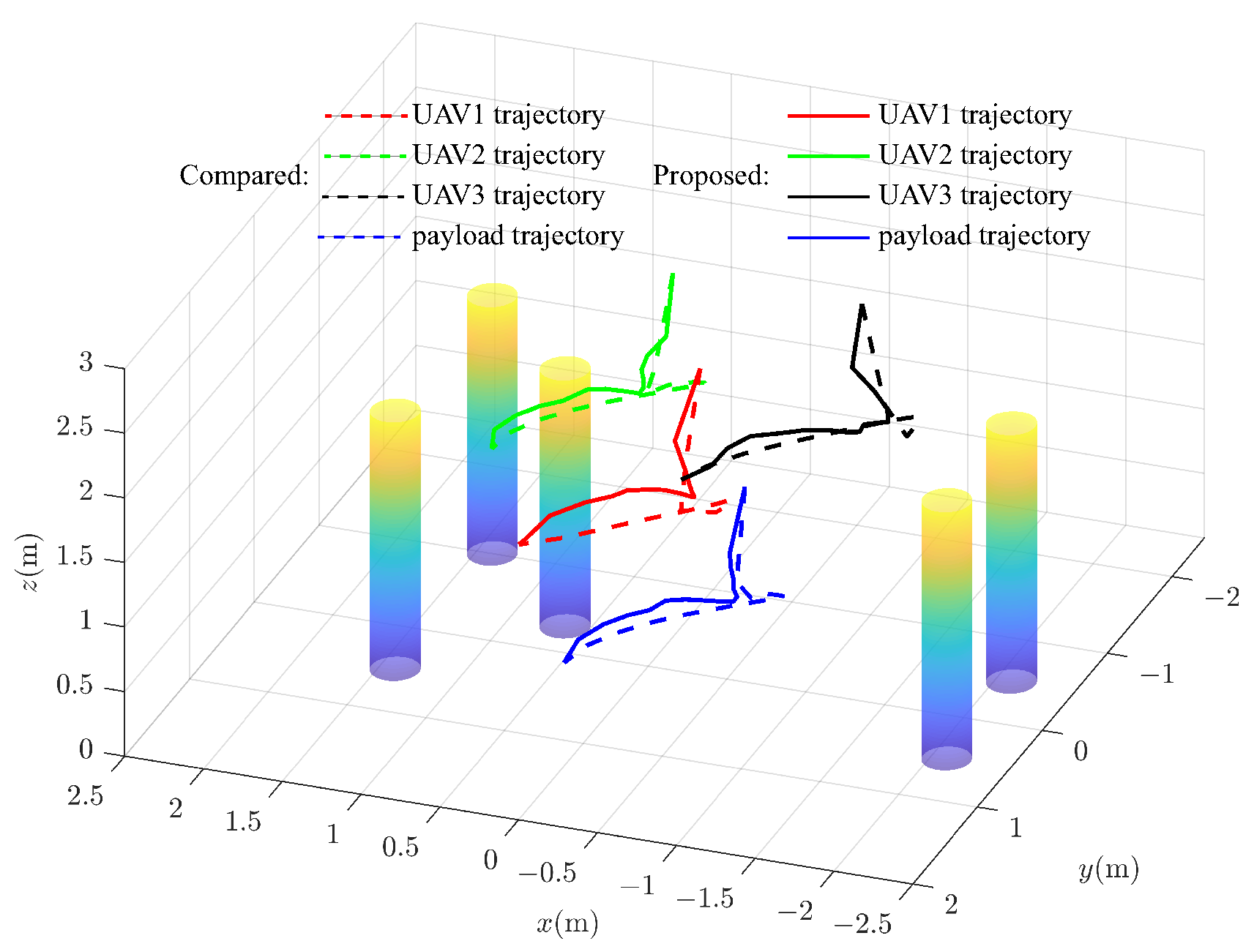
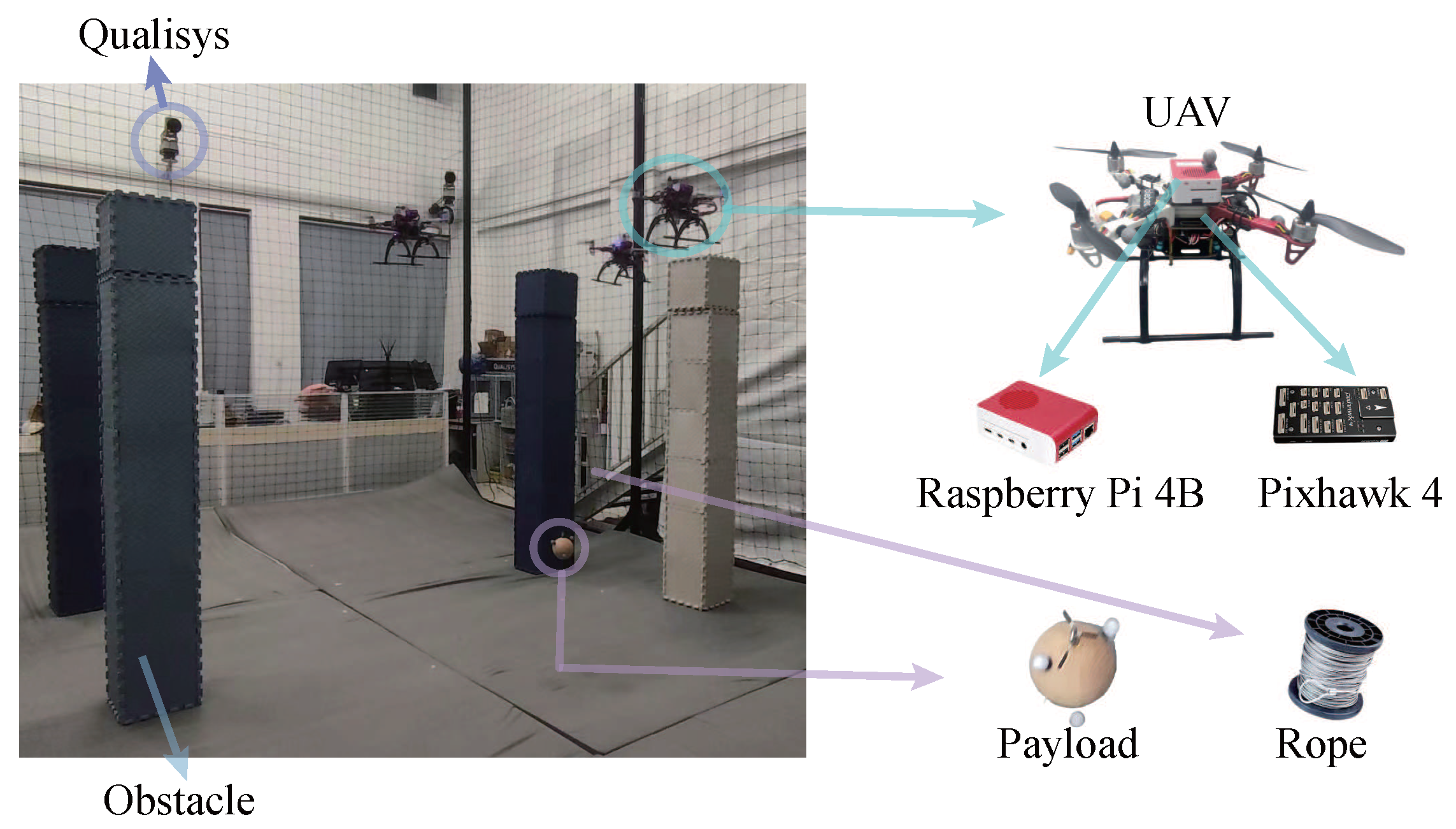
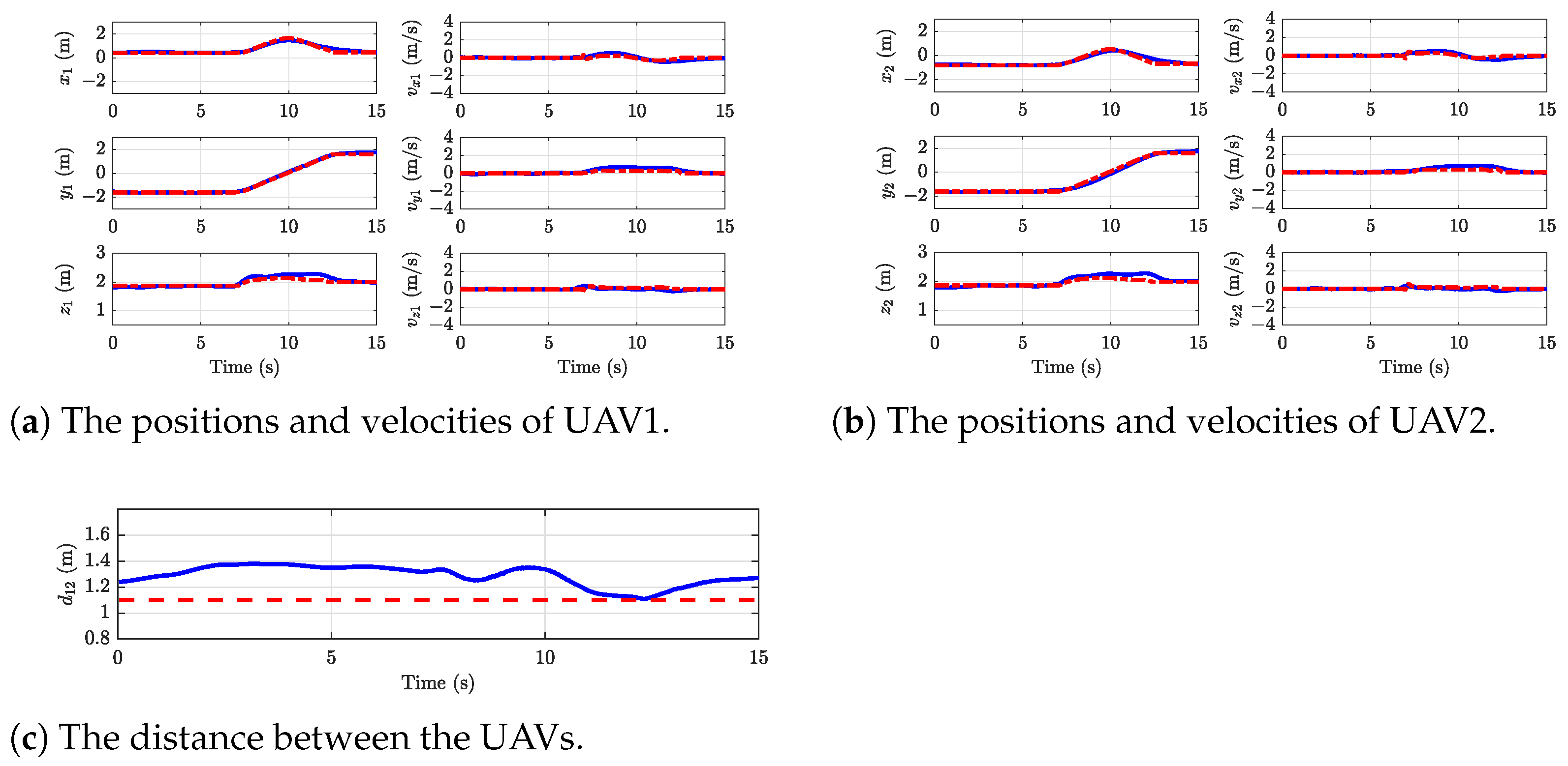
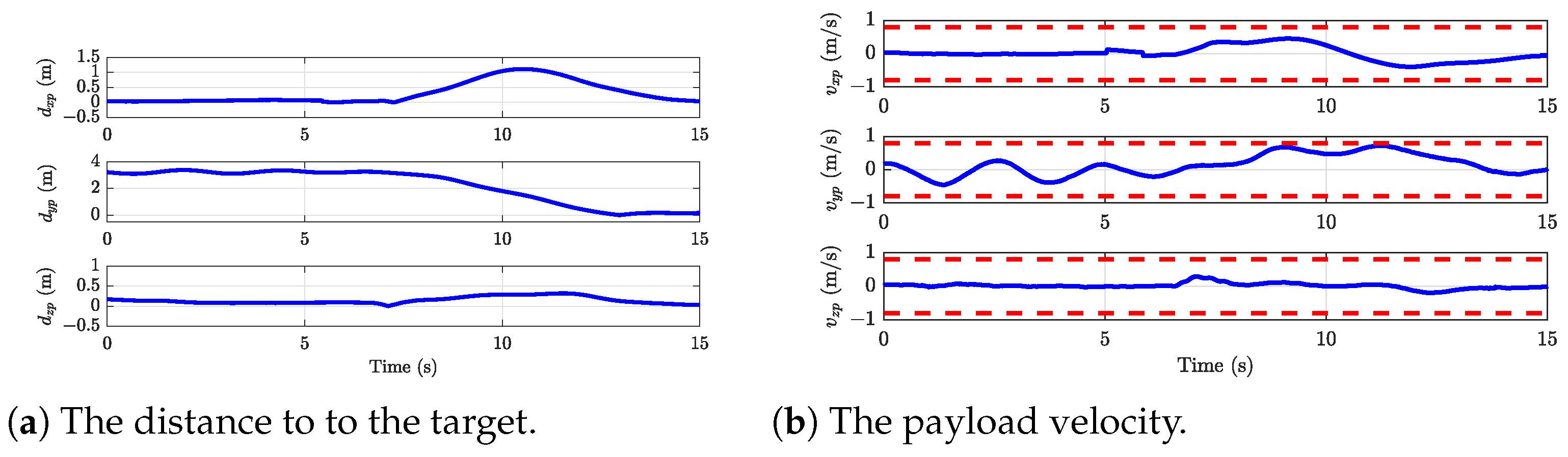
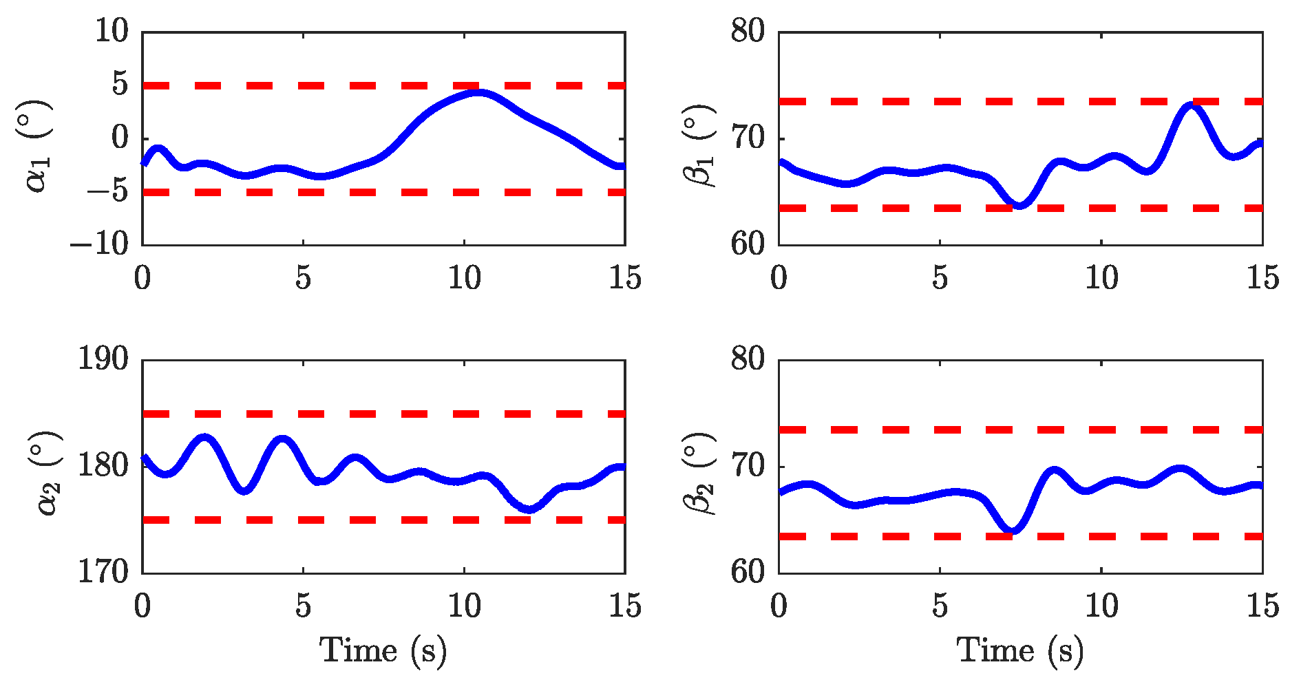
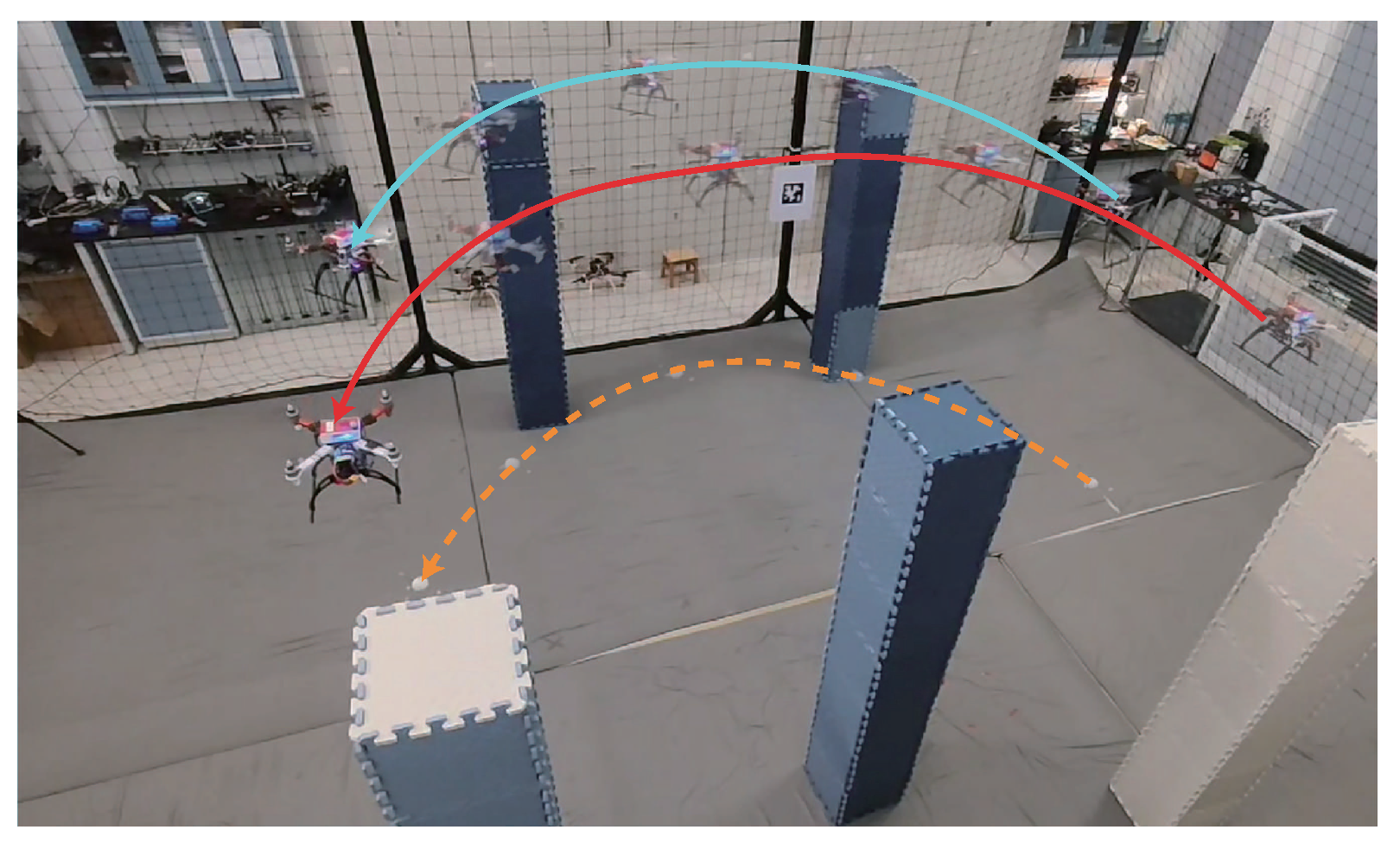
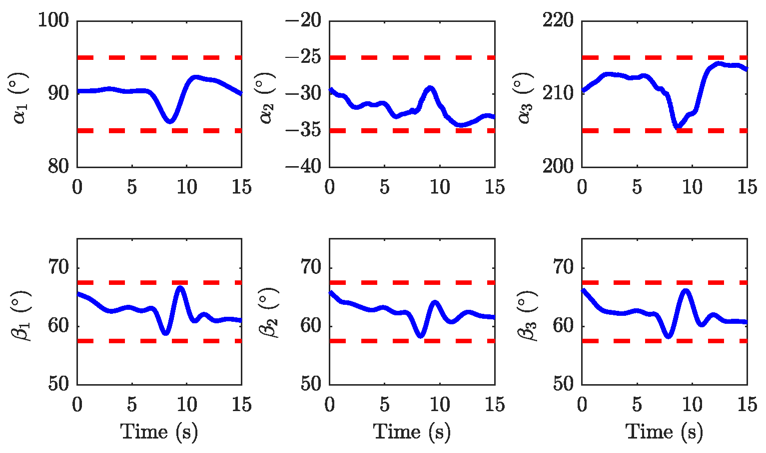
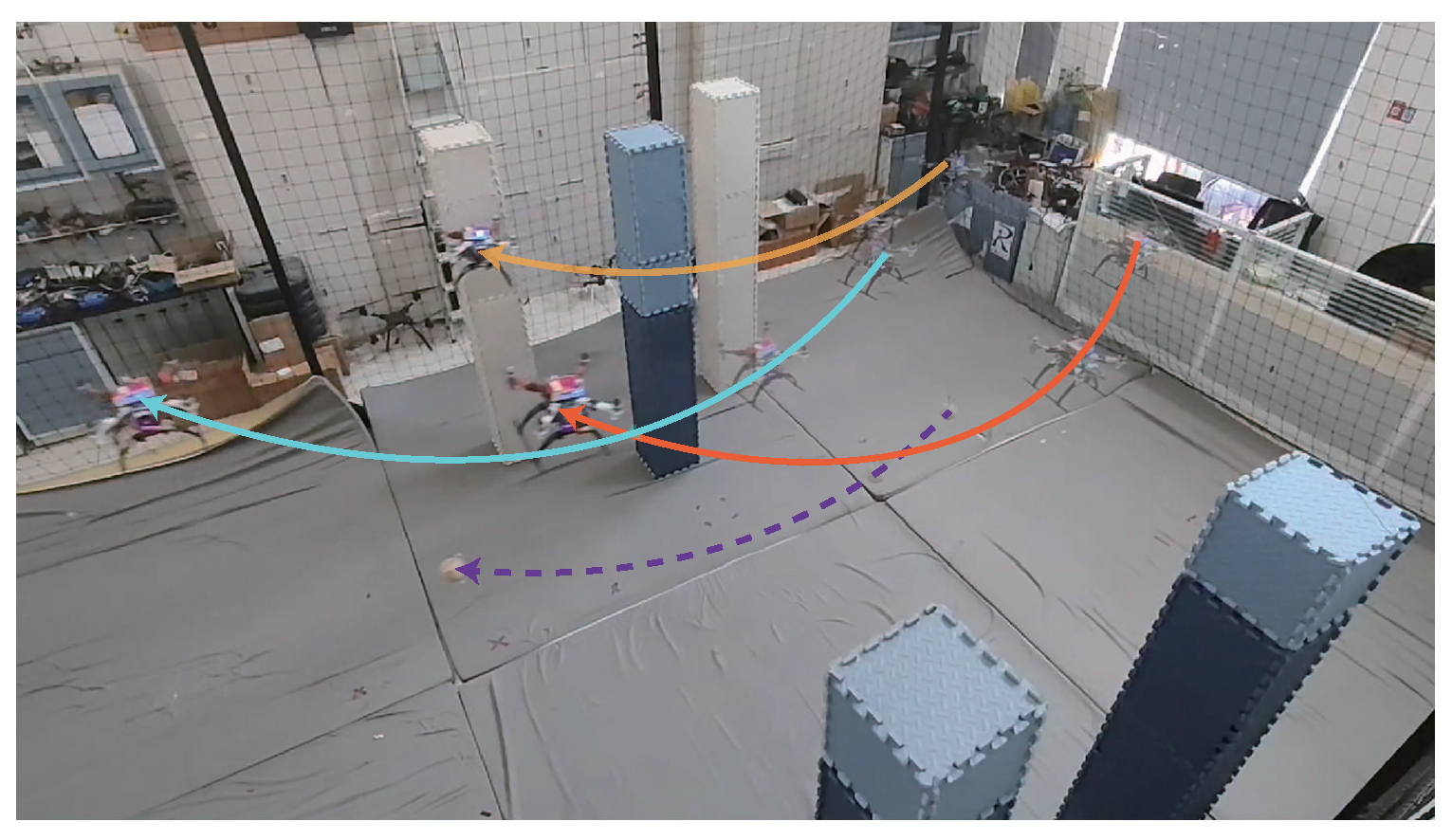
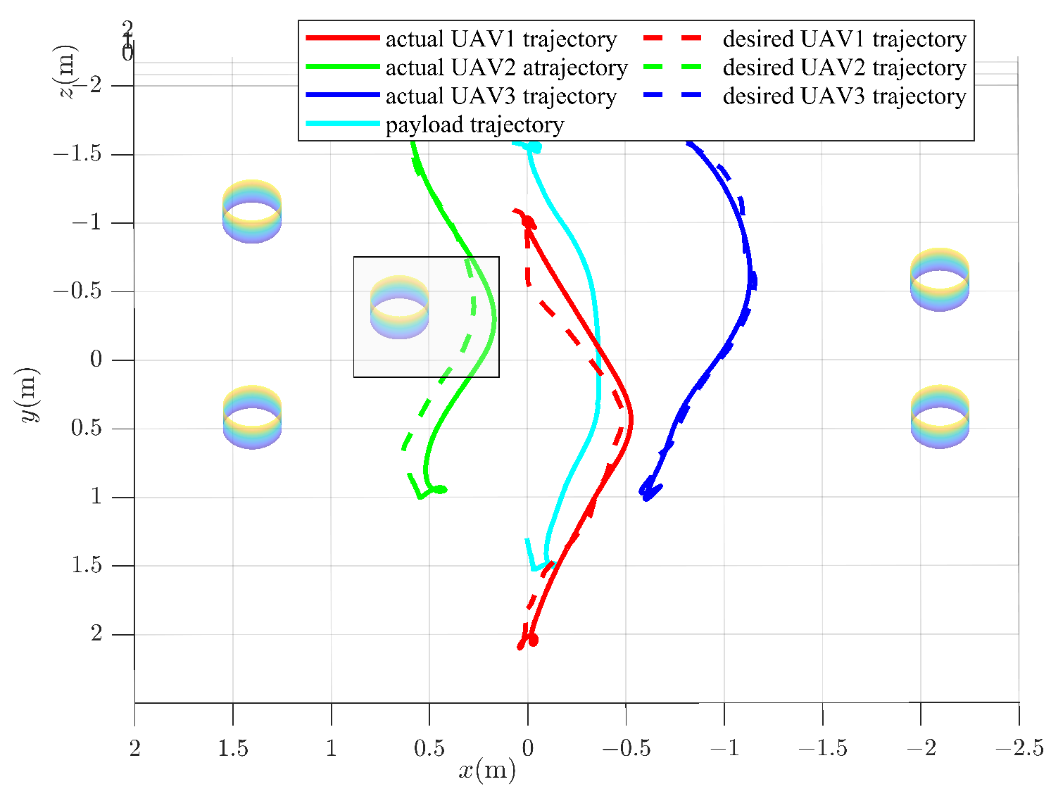
4.2. Experiment
5. Conclusions
Author Contributions
Funding
Data Availability Statement
Conflicts of Interest
References
- Harikumar, K.; Senthilnath, J.; Sundaram, S. Multi-UAV oxyrrhis marina-inspired search and dynamic formation control for forest firefighting. IEEE Trans. Autom. Sci. Eng. 2019, 16, 863–873. [Google Scholar] [CrossRef]
- Wang, J.; Wang, P.; Tian, B. Hyperbolic tangent function-based fixed-time event-triggered control for quadrotor aircraft with prescribed performance. J. Frankl. Inst. 2022, 359, 6267–6285. [Google Scholar] [CrossRef]
- Zhang, J.; Sheng, H.; Chen, Q.; Zhou, H.; Yin, B.; Li, J.; Li, M. A four-dimensional space-time automatic obstacle avoidance trajectory planning method for multi-UAV cooperative formation flight. Drones 2022, 6, 192. [Google Scholar] [CrossRef]
- Shan, L.; Li, H.B.; Miura, R.; Matsuda, T.; Matsumura, T. A novel collision avoidance strategy with D2D communications for UAV systems. Drones 2023, 7, 283. [Google Scholar] [CrossRef]
- Xian, B.; Yang, S. Robust tracking control of a quadrotor unmanned aerial vehicle-suspended payload system. IEEE/ASME Trans. Mechatronics 2020, 26, 2653–2663. [Google Scholar] [CrossRef]
- Li, H.; Zhong, H.; Gao, J.; Lv, Y.; Sha, J.; Liang, J.; Zhang, H.; Wang, Y. A nonlinear trajectory tracking control strategy for quadrotor with suspended payload based on force sensor. IEEE Trans. Intell. Veh. 2024, 9, 704–714. [Google Scholar] [CrossRef]
- Peng, X.; Zhang, Z.; Zhang, A.; Yuen, K.V. Antisaturation backstepping control for quadrotor slung load system with fixed-time prescribed performance. IEEE Trans. Aerosp. Electron. Syst. 2024, 60, 1–12. [Google Scholar] [CrossRef]
- Pounds, P.E.; Dollar, A. Hovering stability of helicopters with elastic constraints. In Proceedings of the Dynamic Systems and Control Conference, Cambridge, MA, USA, 12–15 September 2010; Volume 44182, pp. 781–788. [Google Scholar]
- Backus, S.B.; Odhner, L.U.; Dollar, A.M. Design of hands for aerial manipulation: Actuator number and routing for grasping and perching. In Proceedings of the 2014 IEEE/RSJ International Conference on Intelligent Robots and Systems, Chicago, IL, USA, 14–18 September 2014; pp. 34–40. [Google Scholar]
- Suarez, A.; Jimenez-Cano, A.; Vega, V.; Heredia, G.; Rodriguez-Castaño, A.; Ollero, A. Lightweight and human-size dual arm aerial manipulator. In Proceedings of the 2017 International Conference on Unmanned Aircraft Systems, Miami, FL, USA, 13–16 June 2017; pp. 1778–1784. [Google Scholar]
- Kim, H.; Seo, H.; Choi, S.; Tomlin, C.J.; Kim, H.J. Incorporating safety into parametric dynamic movement primitives. IEEE Robot. Autom. Lett. 2019, 4, 2260–2267. [Google Scholar] [CrossRef]
- Sreenath, K.; Michael, N.; Kumar, V. Trajectory generation and control of a quadrotor with a cable-suspended load-A differentially-flat hybrid system. In Proceedings of the 2013 IEEE International Conference on Robotics and Automation, Karlsruhe, Germany, 6–10 May 2013; pp. 4888–4895. [Google Scholar]
- Tang, S.; Thomas, J.; Kumar, V. Hold or take optimal plan (hoop): A quadratic programming approach to multi-robot trajectory generation. Int. J. Robot. Res. 2018, 37, 1062–1084. [Google Scholar] [CrossRef]
- Kim, H.; Seo, H.; Kim, J.; Kim, H.J. Sampling-based motion planning for aerial pick-and-place. In Proceedings of the 2019 IEEE/RSJ International Conference on Intelligent Robots and Systems, Macau, China, 3–8 November 2019; pp. 7402–7408. [Google Scholar]
- Silveira, J.; Givigi, S.N.; Freire, E.O.; Molina, L.; Carvalho, E. Aggressive motion planning for a quadrotor system with slung load based on RRT. In Proceedings of the 2020 IEEE International Systems Conference, Montreal, QC, Canada, 24 August–20 September 2020; pp. 1–7. [Google Scholar]
- Foehn, P.; Falanga, D.; Kuppuswamy, N.; Tedrake, R.; Scaramuzza, D. Fast trajectory optimization for agile quadrotor maneuvers with a cable-suspended payload. In Proceedings of the Robotics: Science and Systems, Cambridge, MA, USA, 12–16 July 2017. [Google Scholar]
- Zeng, J.; Kotaru, P.; Mueller, M.W.; Sreenath, K. Differential flatness based path planning with direct collocation on hybrid modes for a quadrotor with a cable-suspended payload. IEEE Robot. Autom. Lett. 2020, 5, 3074–3081. [Google Scholar] [CrossRef]
- Hua, H.; Fang, Y.; Zhang, X.; Qian, C. A time-optimal trajectory planning strategy for an aircraft with a suspended payload via optimization and learning approaches. IEEE Trans. Control. Syst. Technol. 2022, 30, 2333–2343. [Google Scholar] [CrossRef]
- Sreenath, K.; Kumar, V. Dynamics, control and planning for cooperative manipulation of payloads suspended by cables from multiple quadrotor robots. Proc. Robot. Sci. Syst. 2013, 1, r3. [Google Scholar]
- Liu, Y.; Zhang, F.; Huang, P.; Zhang, X. Analysis, planning and control for cooperative transportation of tethered multi-rotor UAVs. Aerosp. Sci. Technol. 2021, 113, 106673. [Google Scholar] [CrossRef]
- Geng, J.; Singla, P.; Langelaan, J.W. Load-distribution-based trajectory planning and control for a multilift system. J. Aerosp. Inf. Syst. 2022, 19, 366–381. [Google Scholar] [CrossRef]
- Li, X.; Zhang, J.; Han, J. Trajectory planning of load transportation with multi-quadrotors based on reinforcement learning algorithm. Aerosp. Sci. Technol. 2021, 116, 106887. [Google Scholar] [CrossRef]
- Pei, C.; Zhang, F.; Huang, P.; Yu, H. Trajectory planning for collaborative transportation by tethered multi-UAVs. In Proceedings of the 2021 IEEE International Conference on Real-time Computing and Robotics, Xining, China, 15–19 July 2021; pp. 769–775. [Google Scholar]
- Jackson, B.E.; Howell, T.A.; Shah, K.; Schwager, M.; Manchester, Z. Scalable cooperative transport of cable-suspended loads with UAVs using distributed trajectory optimization. IEEE Robot. Autom. Lett. 2020, 5, 3368–3374. [Google Scholar] [CrossRef]
- Alothman, Y.; Guo, M.; Gu, D. Using iterative LQR to control two quadrotors transporting a cable-suspended load. IFAC-PapersOnLine 2017, 50, 4324–4329. [Google Scholar] [CrossRef]
- Boyd, S.P.; Vandenberghe, L. Convex Optimization; Cambridge University Press: Cambridge, UK, 2004. [Google Scholar]
- Zhang, X.; Liniger, A.; Borrelli, F. Optimization-based collision avoidance. IEEE Trans. Control Syst. Technol. 2020, 29, 972–983. [Google Scholar] [CrossRef]
- Thirugnanam, A.; Zeng, J.; Sreenath, K. Safety-critical control and planning for obstacle avoidance between polytopes with control barrier functions. In Proceedings of the 2022 International Conference on Robotics and Automation, Philadelphia, PA, USA, 23–27 May 2022; pp. 286–292. [Google Scholar]
- Foehn, P.; Romero, A.; Scaramuzza, D. Time-optimal planning for quadrotor waypoint flight. Sci. Robot. 2021, 6, eabh1221. [Google Scholar] [CrossRef] [PubMed]
- Andersson, J.A.E.; Gillis, J.; Horn, G.; Rawlings, J.B.; Diehl, M. CasADi – A software framework for nonlinear optimization and optimal control. Math. Program. Comput. 2019, 11, 1–36. [Google Scholar] [CrossRef]


| Method | Computation Time [s] | Solution [s] |
|---|---|---|
| Relative distance-based method | 95.84 | 5.14 |
| Proposed method | 4.68 | 5.56 |
| Method | Computation Time [s] | Solution [s] |
|---|---|---|
| Relative distance-based method | 44.48 | 3.05 |
| Proposed method | 5.04 | 3.28 |
Disclaimer/Publisher’s Note: The statements, opinions and data contained in all publications are solely those of the individual author(s) and contributor(s) and not of MDPI and/or the editor(s). MDPI and/or the editor(s) disclaim responsibility for any injury to people or property resulting from any ideas, methods, instructions or products referred to in the content. |
© 2024 by the authors. Licensee MDPI, Basel, Switzerland. This article is an open access article distributed under the terms and conditions of the Creative Commons Attribution (CC BY) license (https://creativecommons.org/licenses/by/4.0/).
Share and Cite
Chai, Y.; Liang, X.; Han, J. A Unified Collision Avoidance Trajectory Planning with Dual Variables for Collaborative Aerial Transportation Systems. Drones 2024, 8, 637. https://doi.org/10.3390/drones8110637
Chai Y, Liang X, Han J. A Unified Collision Avoidance Trajectory Planning with Dual Variables for Collaborative Aerial Transportation Systems. Drones. 2024; 8(11):637. https://doi.org/10.3390/drones8110637
Chicago/Turabian StyleChai, Yi, Xiao Liang, and Jianda Han. 2024. "A Unified Collision Avoidance Trajectory Planning with Dual Variables for Collaborative Aerial Transportation Systems" Drones 8, no. 11: 637. https://doi.org/10.3390/drones8110637
APA StyleChai, Y., Liang, X., & Han, J. (2024). A Unified Collision Avoidance Trajectory Planning with Dual Variables for Collaborative Aerial Transportation Systems. Drones, 8(11), 637. https://doi.org/10.3390/drones8110637