Joint Optimization of the 3D Model and 6D Pose for Monocular Pose Estimation

Abstract

The autonomous landing of unmanned aerial vehicles (UAVs) relies on a precise relative 6D pose between platforms. Existing model-based monocular pose estimation methods need an accurate 3D model of the target. They cannot handle the absence of an accurate 3D model. This paper adopts the multi-view geometry constraints within the monocular image sequence to solve the problem. And a novel approach to monocular pose estimation is introduced, which jointly optimizes the target’s 3D model and the relative 6D pose. We propose to represent the target’s 3D model using a set of sparse 3D landmarks. The 2D landmarks are detected in the input image by a trained neural network. Based on the 2D–3D correspondences, the initial pose estimation is obtained by solving the PnP problem. To achieve joint optimization, this paper builds the objective function based on the minimization of the reprojection error. And the correction values of the 3D landmarks and the 6D pose are parameters to be solved in the optimization problem. By solving the optimization problem, the joint optimization of the target’s 3D model and the 6D pose is realized. In addition, a sliding window combined with a keyframe extraction strategy is adopted to speed up the algorithm processing. Experimental results on synthetic and real image sequences show that the proposed method achieves real-time and online high-precision monocular pose estimation with the absence of an accurate 3D model via the joint optimization of the target’s 3D model and pose.

1. Introduction

The autonomous landing of unmanned aerial vehicles (UAVs) necessitates precise estimation of the relative 6D pose, encompassing both 3D rotation and 3D translation [1]. Compared to radar, optoelectronic, and navigation satellite guidance, monocular vision guidance has the advantages of simple configuration, low cost, high autonomy, and strong anti-interference ability. It has received widespread attention from researchers. Monocular pose estimation is one of the critical technologies in monocular vision guidance. Monocular pose estimation, as a significant research direction in the field of computer vision, aims to estimate the position and orientation of a target in three-dimensional space solely based on image information captured by a monocular camera. This technology is not only crucial for applications like autonomous driving and robot navigation but also demonstrates broad application prospects in fields such as augmented reality and virtual reality. Due to complex environmental interference and application conditions, monocular pose estimation remains a challenging task.

Existing monocular pose estimation methods can be divided into cooperative and non-cooperative methods based on whether cooperation markers are used [2]. Cooperative methods [3,4,5] measure the pose by detecting the markers placed on the target. Such methods are simple and efficient. However, the additional cooperation markers limit the application of these methods. On the contrary, non-cooperative methods [6,7,8] only utilize the features of the target itself to achieve pose estimation. And these methods can be further divided into traditional and deep learning-related methods. Traditional methods perform pose estimation based on feature points, templates, etc. [9,10]. They have difficulties dealing with textureless objects, cluttered backgrounds, etc. Benefiting from the powerful feature extraction and representation capabilities of neural networks, deep learning-based methods achieve excellent performance in monocular pose estimation. And they have become the mainstream methods. Some of these methods regress to obtain the pose directly in an end-to-end manner. Such methods are concise, but the accuracy of pose estimation is not high. Some other methods introduce an intermediate representation of the target. The trained networks output the detected intermediate representation. With the accurate 3D prior information of the target, the pose is solved using an Iterative Closest Point (ICP) [11], Perspective-n-Point (PnP) [12,13,14], etc. Existing non-cooperative methods, including traditional and deep learning-related methods, need an accurate 3D model of the target for template preparation, model training, and accurate 2D–3D establishment. However, in practice, due to deviation during the manufacturing process, there are differences between the target entity and its design 3D model. And for sensitive targets, e.g., carrier-borne aircraft or satellites, it is difficult to obtain their accurate 3D models. In the absence of an accurate 3D model of the target, existing methods are unable to achieve high-precision pose estimation.

Multi-view geometry constraints have been widely used in structural reconstruction. Motivated by this, this paper adopts the geometry constraints within the monocular image sequence to handle the problem mentioned above. And a novel method for monocular pose estimation is proposed, which performs joint optimization of the target’s 3D model and pose. Similarly to the landmark used in human pose estimation [15], this paper represents the target’s 3D model using a set of sparse landmarks. A trained neural network is used to detect the landmarks from the input image. With the 2D–3D correspondences, the proposed method obtains the initial pose estimation by solving the PnP problem. Then, for joint optimization, this paper takes the correction value of the landmarks and the pose as parameters to be optimized. We build the optimization objective function based on reprojection errors. By solving this optimization problem, the target’s 3D model and pose are optimized jointly. And we obtain a high-precision pose estimation with the absence of the target’s accurate 3D model. Further, a sliding window combined with a keyframe extraction strategy is also adopted in the proposed method to achieve real-time monocular pose estimation. Experimental results indicate that the proposed method achieves real-time, online, and high-precision monocular pose estimation for the case in which the accurate 3D model is unavailable. And the target’s 3D model is optimized jointly.

The main contributions of this paper are as follows.

1)

To handle the absence of an accurate 3D model, this paper proposes a novel joint opti-mization method of the 3D model and 6D pose for monocular pose estimation. Using the multi-view geometry constraints in a monocular image sequence, it achieves re-al-time, online, and high-precision pose estimation.

2)

This paper proposes to represent the target’s 3D model using a set of sparse landmarks. It enables the joint optimization problem to be efficiently solved.

The rest of the paper is organized as follows: Section 2 gives an overview of the most relevant works to this paper. The proposed method is presented in detail in Section 3. Section 4 describes the experimental results and analysis, and the paper is concluded in Section 5.

2. Related Works

This section summarizes the most related recent works to the proposed method, including deep learning-related monocular pose estimation and multi-view geometry constraints used in 3D structure reconstruction.

2.1. Deep Learning-Related Monocular Pose Estimation

As mentioned above, deep learning-related methods have become the mainstream method in monocular pose estimation. According to whether to use intermediate representation, existing deep learning-related monocular pose estimation methods can be categorized into two main kinds: direct and indirect methods. The direct method [16,17,18] takes the input image and regresses it to obtain the pose parameters directly. Kendall et al. [18] proposed PoseNet, which trained a convolutional neural network to regress the 6-DOF camera pose from a single RGB image. The direct method achieves end-to-end network training and inference, but the precision of pose estimation is not high. The indirect method introduces an intermediate representation of the target. By inferring intermediate representation, the indirect method adopts PnP, ICP, etc., to solve pose parameters. Common intermediate models include dense models, normalized coordinates, and sparse landmarks. The dense model-based pose estimation method [19,20,21] matches each pixel in the image or scene. For instance, DPOD [20] estimated dense multiclass 2D–3D mappings between the input image and the available 3D model. The dense model-based representation method has high accuracy and stability, but low computational efficiency. The normalized coordinates-based method [22,23,24,25] normalized objects belonging to the same category through normalized object coordinate space. And it does not need to obtain an accurate 3D model of the target. However, the normalized coordinates-based method relies on the depth image to restore the true scale of the object. The sparse landmarks representation method [26,27,28,29,30,31,32] models the object as a sparse landmark set. And it is simple and efficient, suitable for real-time pose estimation tasks. At present, the sparse landmarks representation method is widely used. By establishing sparse or dense 2D–3D correspondence, the indirect method can solve PnP to obtain a more accurate pose than the direct method. Although indirect methods perform better, the non-differentiable nature limits their application in pose estimation tasks. To solve this problem, Chen et al. [33] and EPro-PnP [34] interpreted PnP as a differentiable layer embedded into the neural network. With a differentiable PnP layer, end-to-end training of the indirect method is achieved. In addition, multi-view geometry constraints have been applied in monocular pose estimation [35,36]. For example, CosyPose [36] realized global scene optimization through object-level bundle adjustment.

The above methods all require accurate target 3D prior information, such as an accurate 3D CAD model. Through 3D prior information, 2D–3D correspondences or 3D-3D correspondences are established to achieve accurate pose estimation. However, they cannot handle the case in which the accurate target’s 3D model is absent.

2.2. Multi-View Geometry Constraints

Multi-view geometry constraints recover the 3D structure of the object or scene using the internal relationship between the images and calculate the camera pose simultaneously, e.g., Simultaneous Localization and Mapping (SLAM) [37,38,39,40], Structure from Motion (SfM) [41,42], object localization [43], and high-precision localization of the aircraft itself [44]. Similarly, in the monocular pose estimation focused on in this paper, the image sequence provides multi-view geometry constraints due to the presence of relative motion. Therefore, in this paper, we attempt to use multi-view geometry constraints to handle the monocular pose estimation in the absence of the accurate target’s 3D model. It should be noted that our method is different from the traditional SLAM and SfM methods. These methods all utilize feature point extraction and matching to establish inter-frame matching and then solve the pose and localization by optimization. However, the target’s 3D platform we focus on cannot establish correspondences based on traditional feature points. Furthermore, even when feature point correspondences are established, linking them to specific 3D models remains challenging. Therefore, in this paper, complex feature point extraction and matching methods are discarded, and an existing neural network-based landmark detection algorithm is used to directly regress the 2D projections corresponding to predefined 3D landmarks.

3. Method

To achieve reliable monocular pose estimation for UAV autonomous landing missions without an accurate 3D model, this paper proposes a novel joint optimization method using multi-view geometry constraints within image sequences. In this section, we first describe the joint optimization problem and notations. Then, the proposed method is provided in detail in Section 3.2.

3.1. Problem Formulation and Notations

A basic schematic of the object imaging and monocular pose estimation process is given in Figure 1, where $O_O-X_O{Y}_O{Z}_O$ and $O_C-X_C{Y}_C{Z}_C$ denote the target coordinate frame and camera coordinate frame, respectively.

In Figure 1, the rigid body transformation from the target coordinate frame to the camera coordinate frame is represented by ${\mathit{T}}_{\mathrm{O}}^{\mathrm{C}}$, i.e.,

$${\mathit{T}}_{\mathrm{O}}^{\mathrm{C}}=\left[\begin{array}{cc}{\mathit{R}}_{\mathrm{O}}^{\mathrm{C}}& {\mathit{t}}_{\mathrm{O}}^{\mathrm{C}}\\ \mathbf{0}& 1\end{array}\right]\in \mathbb{SE}\left(3\right),{\mathit{R}}_{\mathrm{O}}^{\mathrm{C}}\in \mathbb{SO}\left(3\right),{\mathit{t}}_{\mathrm{O}}^{\mathrm{C}}\in {\mathbb{R}}^3$$

(1)

where the symbols $\mathbb{S}\mathbb{E}(3)$ and $\mathbb{S}\mathbb{O}(3)$ used in this article denote the special Euclidean group and the special orthogonal group, respectively [45]. ${\mathit{R}}_{\mathrm{O}}^{\mathrm{C}}$ and ${\mathit{t}}_{\mathrm{O}}^{\mathrm{C}}$ are the rotation and translation components of ${\mathit{T}}_{\mathrm{O}}^{\mathrm{C}}$, respectively.

The perspective projection of a vertex ${\tilde{\mathit{V}}}^{\mathrm{O}}=\left[v_x^{\mathrm{O}}{v}_y^{\mathrm{O}}{v}_z^{\mathrm{O}}1\right]$ of the target’s 3D model onto a 2D image can be modeled as follows:

$$\mathit{x}=\mathit{\pi }\left(\mathit{K}{\left({\mathit{T}}_{\mathrm{O}}^{\mathrm{C}}{\tilde{\mathit{V}}}^{\mathrm{O}}\right)}_{3\times 1}\right)$$

(2)

with $\mathit{K}$ representing the precalibrated and fixed $3\times 3$ camera intrinsic matrix, $\mathit{x}={\left[uv\right]}^{\mathrm{T}}$ the image point. In $\mathit{x}={\left[uv\right]}^{\mathrm{T}}$, $u$ and $v$ represent the pixel coordinates of $\mathit{x}$ on the horizontal and vertical axes, respectively. $\mathit{\pi }\left(\mathit{X}\right)={\left[x/zy/z\right]}^{\mathrm{T}}$ and $\mathit{X}=\left[xyz\right]$ are the homogeneous coordinates of the image point $\mathit{x}$.

Monocular pose estimation extracts 2D features in the image and combines the target’s accurate 3D information to establish the 2D–3D correspondence for solving 6D pose. Hence, the inaccurate 3D model makes it difficult to solve the pose for existing methods. To be specific, there is a difference between the obtained target’s 3D model ${\mathit{X}}^{\mathrm{O}}$ and the accurate target’s 3D model $\overline{{\mathit{X}}^{\mathrm{O}}}$. And the 3D model error is denoted as $\mathrm{\Delta }{\mathit{X}}^{\mathrm{O}}$, so, ${\mathit{X}}^{\mathrm{O}}=\overline{{\mathit{X}}^{\mathrm{O}}}+\mathrm{\Delta }{\mathit{X}}^{\mathrm{O}}$. The traditional methods cannot obtain accurate pose by utilizing ${\mathit{X}}^{\mathrm{O}}$. Therefore, this paper aims to address the problem of monocular pose estimation in the absence of an accurate 3D model. And the solution of the 3D model and pose is realized by the method of joint optimization.

3.2. Joint Optimization of the 3D Model and Pose for Monocular Pose Estimation

This paper proposes to represent the target’s 3D model using a set of sparse 3D landmarks. The initial pose is obtained by detecting 2D landmarks combined with solving the PnP problem. And the pose and 3D model are jointly optimized via bundle adjustment. As shown in Figure 2, the proposed monocular pose estimation method mainly includes sparse landmark-based 3D model representation, initial pose estimation, joint optimization of the 3D model and pose, and sliding window combined with keyframe extraction strategy, which are all described in detail next.

3.2.1. Sparse Landmark-Based 3D Model Representation

In this paper, the pose measurement in the visual guidance of UAV autonomous landing is used as an example to illustrate the proposed method. And the ship shown in Figure 3 is used as the target platform. In Figure 3b, the 3D model is obtained by accurate 3D scanning of the simplified physical model of the ship. As shown in Figure 3b, to make the proposed joint optimization method efficient and reliable, a set of sparse 3D landmarks capable of representing the main structure of the ship is employed to represent the target’s 3D model. Different from the 2D feature points used in traditional SLAM, SfM, and other fields, this paper uses semantic-level landmarks to represent the target’s 3D model.

Furthermore, this paper uses ${\tilde{\mathit{X}}}^{\mathrm{O}}$ to represent a set of sparse landmarks used, as shown in Equation (3):

$${\left\{{\tilde{\mathit{X}}}_j^{\mathrm{O}}\right\}}_{j=1,2,...,N}={\left\{{\left[x_j^{\mathrm{O}}{y}_j^{\mathrm{O}}{z}_j^{\mathrm{O}}1\right]}^{\mathrm{T}}\right\}}_{j=1,2,...,N}$$

(3)

where $N$ is 13 and represents the number of 3D landmarks used. To simulate the dual-motion platform rendezvous in the actual task, we scaled the 3D landmark coordinates of the ship to the actual size.

3.2.2. Initial Pose Estimation Based on the Set of Sparse Landmarks

As shown in Figure 4, the initial pose estimation part provides the initial pose for the subsequent optimization. Specifically, this paper performs target detection on the initial frame. Subsequently, the 2D landmarks are detected within the target region, and the initial pose is obtained by solving the PnP problem. For efficiency, a 2D target tracking algorithm is adopted in subsequent frames. In addition, to improve the robustness of the initial pose estimation, we design a consistency criterion to determine the success or failure of the 2D tracking and pose estimation.

A.

2D landmark detection

YOLOX employs a lightweight network architecture, which grants it a notable advantage in computational speed. Compared to other object detection algorithms, YOLOX achieves faster object detection while maintaining accuracy, making it suitable for application scenarios with high real-time requirements. Therefore, as shown in Figure 4, this paper utilizes the YOLOX algorithm [46] to detect the target position. The YOLOX outputs the target box region in the image, denoted as B. YOLOX takes more time to detect the target on a single frame. Hence, to improve efficiency, after obtaining the target area in the initial frame, the STAPLE algorithm [47] is utilized to track the target from the subsequent input images. To keep the notation uniform, the target box region output by the STAPLE algorithm is also denoted as B. Then, based on the representation of the sparse landmark set proposed in Section 3.2.1, the RTMPose algorithm, according to ref. [48], with superior performance in human pose estimation tasks, is utilized to realize the efficient and accurate detection of 2D landmarks in the input image. The RTMPose algorithm outputs the positions of 2D landmarks through heat maps, which are concise, efficient, and easy to deploy. Actually, this approach presented in this paper can incorporate a variety of efficient and precise landmark detection methods, rather than being confined merely to RTMPose. Finally, the paper utilizes the EPnP [12] + RANSAC [49] method to solve the initial pose.

For training, this paper first adopts a manual method to annotate the coordinates of sparse landmarks on a single image as the ground truth. Subsequently, the annotated data are divided into a training set and a validation set, which are then fed into the network for training. Eventually, a 2D landmark detection model is obtained. It is important to note that the RTMPose algorithm is an instance-level landmark detection algorithm. Therefore, it requires separate training for each individual object to obtain the corresponding landmark detection model. This approach limits the generalization ability of the proposed method. Therefore, the next step of this paper is to explore category-level landmark detection algorithms.

B.

Consistency criteria

After solving the pose, this paper further calculates the intersection ratio $I$ between B and the target’s 3D landmark reprojection bounding box $B_r$. By $B_r$, the proposed method determines whether the solved initial pose is reliable, as shown in Equation (4).

$$I={\displaystyle \frac{B\cap B_r}{B_r}}$$

(4)

When $I<Threshold$, i.e., $B_r\not\subset B$, the solved pose is considered unreliable. Then, the current frame is processed according to the initial frame and the pose is re-solved. Otherwise, subsequent joint optimization operations are performed.

3.2.3. Joint Optimization of the 3D Model and 6D Pose

Based on the initial pose estimation results obtained above, in this section, the correction value $\mathrm{\Delta }{\mathit{X}}^{\mathrm{O}}$ of the target’s 3D model ${\mathit{X}}^{\mathrm{O}}$ and the initial pose estimation ${\left\{{\mathit{T}}_{\mathrm{O}}^{{\mathrm{C}}_i}\right\}}_{i=1:M}$ of consecutive M frames are taken as the parameters to be optimized. And the optimization objective function is established by minimizing the reprojection error, as shown in Equation (5):

$$\left\{\begin{array}{l}\mathrm{\Delta }{\mathit{X}}^{\mathrm{O}*},{\mathit{T}}_{\mathrm{O}}^{\mathrm{C}*}=\arg \underset{\mathrm{\Delta }{\mathit{X}}^{\mathrm{O}},{\mathit{T}}_{\mathrm{O}}^{\mathrm{C}}}{\min }{\displaystyle \frac{1}{2}}{{\displaystyle \sum _{i=1}^M{\displaystyle \sum _{j=1}^N‖{\mathit{x}}_i^j-\pi \left(\mathit{K}{\left({\mathit{T}}_{\mathrm{O}}^{{\mathrm{C}}_i}\left({\tilde{\mathit{X}}}_j^{\mathrm{O}}+\mathrm{\Delta }{\tilde{\mathit{X}}}_j^{\mathrm{O}}\right)\right)}_{3\times 1}\right)‖}}}_2^2\hfill \\ {\mathit{X}}^{\mathrm{O}*}={\mathit{X}}^{\mathrm{O}}+\mathrm{\Delta }{\mathit{X}}^{\mathrm{O}*}\hfill \end{array}\right.$$

(5)

where ${‖.‖}_2^2$ represents the square of the vector norm. $\mathrm{\Delta }{\mathit{X}}^{\mathrm{O}*}$ is the optimized correction value of the 3D model. ${\mathit{X}}^{\mathrm{O}*}={\left\{{\mathit{X}}_j^{\mathrm{O}*}\right\}}_{j=1,2,...,N}$ and ${\mathit{T}}_{\mathrm{O}}^{\mathrm{C}*}={\left\{{\mathit{T}}_{\mathrm{O}}^{{\mathrm{C}}_i^{*}}\right\}}_{i=1,2,...,M}$ are the optimized 3D model and pose, respectively. Furthermore, $x_i^j$ is the observed value of the $j^{th}$ 3D landmark on the $i^{th}$ frame. ${\tilde{\mathit{X}}}_j^{\mathrm{O}}$ is the original homogeneous coordinate of the $j^{th}$ 3D landmark. $\mathrm{\Delta }{\tilde{\mathit{X}}}_j^{\mathrm{O}}$ is the homogeneous coordinate of the correction value to be optimized of the $j^{th}$ 3D landmark. ${\mathit{T}}_{\mathrm{O}}^{{\mathrm{C}}_i}$ is the pose to be optimized for the $i^{th}$ frame, which can be modeled with a twist $\xi \in {ℝ}^6$, as follows:

$${\mathit{T}}_{\mathrm{O}}^{{\mathrm{C}}_i}=\exp \left(\widehat{\xi }\right)$$

(6)

where

$$\left\{\begin{array}{l}\xi =\left[\begin{array}{c}\mathit{\varphi }\\ \mathit{\rho }\end{array}\right]={\left[\begin{array}{cccc}{\varphi }_1& {\varphi }_2& {\varphi }_3& \begin{array}{cc}{\rho }_1& \begin{array}{cc}{\rho }_2& {\rho }_3\end{array}\end{array}\end{array}\right]}^{\mathrm{T}}\in \mathfrak{s}\mathfrak{e}\left(3\right)\hfill \\ \widehat{\xi }=\left[\begin{array}{cc}\widehat{\mathit{\varphi }}& \mathit{\rho }\\ {\mathbf{0}}^{\mathrm{T}}& 0\end{array}\right]\in {ℝ}^{4\times 4},\mathit{\varphi }\in \mathfrak{s}\mathfrak{o}\left(3\right),\mathit{\rho }\in {ℝ}^3\hfill \end{array}\right.$$

(7)

where $\mathfrak{s}\mathfrak{e}\left(3\right)$ is the Lie algebra corresponding to $\mathbb{S}\mathbb{E}(3)$, and $\mathfrak{s}\mathfrak{o}\left(3\right)$ is the Lie algebra corresponding to $\mathbb{S}\mathbb{O}(3)$ [45]. The rotation and translation components of the $\mathfrak{s}\mathfrak{e}\left(3\right)$ are $\mathit{\varphi }\in \mathfrak{s}\mathfrak{o}\left(3\right)$ and $\mathit{\rho }\in {ℝ}^3$, respectively [45]. And $\widehat{\mathit{\varphi }}$ represents the skew-symmetric defined by $\mathit{\varphi }$.

In this paper, we focus on monocular pose estimation in the absence of an accurate 3D model. During the optimization process, the amount of the correction value of the model is constrained. This is mainly because the gap between the 3D model and the real object is relatively small in practice. Therefore, the search space in the optimization can be limited by constraining the optimization range of the correction value. It prevents the algorithm from becoming stuck in the local optimal solution and makes the optimized 3D model closer to the actual situation. When the deviation between the 3D model and the real object is large, it is difficult to reduce the model error by joint optimization. And this paper does not focus on the optimization of 3D models with excessive errors. Hence, the correction value threshold ${\sigma }_1$ of the target’s 3D model is set. After optimization, when $\mathrm{\Delta }{\mathit{X}}^{\mathrm{O}*}$ exceeds ${\sigma }_1$, the optimization result of the 3D model is discarded, as shown in Equation (8).

$$\mathrm{\Delta }{\mathit{X}}^{\mathrm{O}*}=\left\{\begin{array}{l}\mathrm{\Delta }{\mathit{X}}^{\mathrm{O}*},if{‖\mathrm{\Delta }{\mathit{X}}^{\mathrm{O}*}‖}_2\le {\sigma }_1\hfill \\ 0,else\hfill \end{array}\right.$$

(8)

In addition, the poses obtained by joint optimization can be output directly as the final measurement result. However, the poses direct output from optimization may not be accurate. Therefore, this paper solves the PnP problem again using the optimized 3D model to obtain the final pose estimation result $\widehat{{\mathit{T}}_{\mathrm{O}}^{{\mathrm{C}}_{\mathrm{c}\mathrm{u}\mathrm{r}}}}$ for the current frame.

3.2.4. Sliding Window Combined with Keyframe Extraction Strategy

In Section 3.2.3, based on Equations (5) and (8), the 6D pose for each input image and 3D model are continuously jointly optimized to obtain a high-precision pose and reduce 3D model error. However, monocular visual guidance requires real-time, online, and continuous pose measurement. In Section 3.2.3, the number of consecutive images increases over time. And, in the established optimization objective function, the residual error and the pose optimization parameters are continuously increased. Therefore, in Section 3.2.4, this paper uses the sliding window strategy instead of the frame-by-frame optimization strategy to restrict the optimization scale. It only optimizes the pose of the image within a time window of a fixed length $L$.

The adoption of the sliding window strategy can effectively reduce the computational scale of the process to be optimized. However, the amount of pose variation between consecutive frames is small, and the provided geometry constraints are not enough. Therefore, to take advantage of stronger geometry constraints and improve the processing efficiency, after utilizing a sliding window, this paper further adopts the processing strategy of keyframes in the proposed optimization method. Referring to the keyframe extraction strategy in ORB-SLAM2 [40], this paper selects keyframes in the input image sequence. Then, the poses of the extracted keyframes and the correction value of the target’s 3D model are taken as the parameters to be optimized. If the current frame is a non-keyframe, the PnP problem is calculated using the recently optimized target’s 3D model to obtain its high-precision pose. In detail, we select keyframes according to the camera rotation angle, as shown in Figure 5. This paper assumes that the existing keyframe set is ${\mathit{F}}_{\mathrm{k}\mathrm{e}\mathrm{y}}=\left\{{\mathit{F}}_{\mathrm{k}\mathrm{e}\mathrm{y}}^0,{\mathit{F}}_{\mathrm{k}\mathrm{e}\mathrm{y}}^1,...,{\mathit{F}}_{\mathrm{k}\mathrm{e}\mathrm{y}}^{k-1}\right\}$ and its corresponding pose set is ${\mathit{T}}_{\mathrm{O}}^{{\mathrm{C}}_{\mathrm{k}\mathrm{e}\mathrm{y}}}=\left\{{\mathit{T}}_{\mathrm{O}}^{{\mathrm{C}}_{\mathrm{k}\mathrm{e}\mathrm{y}}^0},{\mathit{T}}_{\mathrm{O}}^{{\mathrm{C}}_{\mathrm{k}\mathrm{e}\mathrm{y}}^1},...,{\mathit{T}}_{\mathrm{O}}^{{\mathrm{C}}_{\mathrm{k}\mathrm{e}\mathrm{y}}^{k-1}}\right\}$. The origin of the current frame’s camera and the nearest keyframe’s camera are connected with the origin of the target coordinate frame, respectively. And the two connections are $\overrightarrow{{\mathit{OF}}_{\mathrm{k}\mathrm{e}\mathrm{y}}^{k-1}}$ and $\overrightarrow{{\mathit{OF}}_{\mathrm{c}\mathrm{u}\mathrm{r}}}$ in Figure 5, respectively. Then, the angle $\omega$ between the two vectors is calculated according to Equations (9) and (10). When $\omega$ is greater than the angle threshold ${\omega }_{\min }$, the current frame will be added to the set of keyframes.

$$\left\{\begin{array}{c}\overrightarrow{{\mathit{OF}}_{\mathrm{k}\mathrm{e}\mathrm{y}}^{k-1}}=-{({\mathit{R}}_{\mathrm{O}}^{{\mathrm{C}}_{\mathrm{k}\mathrm{e}\mathrm{y}}^{k-1}})}^{\mathrm{T}}{\mathit{t}}_{\mathrm{O}}^{{\mathrm{C}}_{\mathrm{k}\mathrm{e}\mathrm{y}}^{k-1}}\\ \overrightarrow{{\mathit{OF}}_{\mathrm{c}\mathrm{u}\mathrm{r}}}=-{({\mathit{R}}_{\mathrm{O}}^{{\mathrm{C}}_{\mathrm{c}\mathrm{u}\mathrm{r}}})}^{\mathrm{T}}{\mathit{t}}_{\mathrm{O}}^{{\mathrm{C}}_{\mathrm{c}\mathrm{u}\mathrm{r}}}\end{array}\right.$$

(9)

$$\omega =arc\cos \left({\displaystyle \frac{\overrightarrow{{\mathit{OF}}_{\mathrm{k}\mathrm{e}\mathrm{y}}^{k-1}}.\overrightarrow{{\mathit{OF}}_{\mathrm{c}\mathrm{u}\mathrm{r}}}}{‖\overrightarrow{{\mathit{OF}}_{\mathrm{k}\mathrm{e}\mathrm{y}}^{k-1}}‖‖\overrightarrow{{\mathit{OF}}_{\mathrm{c}\mathrm{u}\mathrm{r}}}‖}}\right)$$

(10)

By setting the sliding window combined with the keyframe extraction strategy, the complexity of the algorithm implementation is reduced, and the efficiency of the algorithm is improved. Hence, Equation (5) is modified as follows:

$$\left\{\begin{array}{l}\mathrm{\Delta }{\mathit{X}}^{\mathrm{O}*},{\mathit{T}}_{\mathrm{O}}^{{\mathrm{C}}_{\mathrm{k}\mathrm{e}\mathrm{y}}^{*}}=\arg \underset{\mathrm{\Delta }{\mathit{X}}^{\mathrm{O}},{\mathit{T}}_{\mathrm{O}}^{{\mathrm{C}}_{\mathrm{k}\mathrm{e}\mathrm{y}}}}{\min }{\displaystyle \frac{1}{2}}{{\displaystyle \sum _{i=0}^L{\displaystyle \sum _{j=1}^N‖{\mathit{x}}_i^j-\pi \left(\mathit{K}{\left({\mathit{T}}_{\mathrm{O}}^{{\mathrm{C}}_{\mathrm{k}\mathrm{e}\mathrm{y}}^i}\left({\tilde{\mathit{X}}}_j^{\mathrm{O}}+\mathrm{\Delta }{\tilde{\mathit{X}}}_j^{\mathrm{O}}\right)\right)}_{3\times 1}\right)‖}}}_2^2\hfill \\ {\mathit{X}}^{\mathrm{O}*}={\mathit{X}}^{\mathrm{O}}+\mathrm{\Delta }{\mathit{X}}^{\mathrm{O}*}\hfill \end{array}\right.$$

(11)

4. Experimental Results and Analysis

To evaluate the performance of the proposed method, this paper implements experiments using both synthetic and real image sequences. This section first describes the experimental settings. Subsequently, the robustness of the proposed method on the simulation data is analyzed. Further, the performance of the proposed method on the 3D model and 6D pose is evaluated on synthetic and real image sequences. Finally, the shortcomings of the proposed method and future improvements are demonstrated.

4.1. Experiment Settings

4.1.1. Training Details Based on Deep Learning Methods

In the synthetic experiment and real experiment detailed below, the automatic landing process of the UAV was simulated from approximately about 2.0 km to 0.2 km distance, respectively. Based on the set camera trajectory, the synthetic images are generated by combining a target’s 3D model with a computer graphics engine. This paper rendered about 16,000 synthetic images with a resolution of 1024 × 1024 pixels. In the real experiment, the size of the target ship model is about 113 mm × 120 mm × 440 mm. This paper simulates the process of a UAV approaching a ship using a handheld camera. In total, about 9000 real images with a resolution of 1280 × 720 pixels were generated. Subsequently, about 13,000 synthetic images and nearly 8000 real images were fed into the network for training, with the remaining images serving as a test set. As for the parameters of deep learning networks, this paper only modifies the output dimension of RTMPose to the number of setting landmarks.

All experiments were conducted on a laptop equipped with an AMD Core R7-5800H @ 3.2 GHz and an NVIDIA Geforce RTX3060 GPU. The GPU was utilized for rendering, training, and inference. Our method is implemented in C++14.

4.1.2. Parameter Settings

In the experiment, uniform distribution can better control the error degree of the target’s 3D model. Therefore, to simulate the absence of an accurate 3D model, this paper adds error to the three dimensions of each accurate 3D landmark by uniform distribution $U\left(a,b\right)$, where $U\left(a,b\right)$ is equal to $U\left(2,3\right)$ or $U\left(-3,-2\right)$. The detailed parameter settings of the proposed method are shown in

Table 1. Parameter settings of the proposed method on synthetic and real experiments.

Parameter	Setting
Consistency criterion threshold	0.8
Correction value threshold ${\sigma }_1$	5
$\mathrm{Angle}\mathrm{threshold}\mathrm{for}\mathrm{keyframe}\mathrm{selecting}{\omega }_{\min }$	Set the appropriate value according to the rendezvous angle of the image sequence
Sliding window length $L$	20

. It should be noted that, in the synthetic experiment, to ensure the selection of sufficient keyframes for optimization while considering efficiency, this paper sets appropriate keyframe selection threshold ${\omega }_{\min }$ based on the rendezvous angles of different image sequences.

4.1.3. Evaluation Metrics

To evaluate the performance of different landmark detection algorithms, this paper uses Normalized Mean Error [50] (NME) to calculate 2D landmark detection error, as shown in Equation (12):

$$\mathrm{N}\mathrm{M}\mathrm{E}=\mathbb{E}\left({\displaystyle \frac{{‖{\mathit{x}}_j^{\mathrm{p}}-{\mathit{x}}_j^{\mathrm{g}}‖}_2}{\sqrt{wh}}}\right)$$

(12)

where $\mathbb{E}\left(.\right)$ indicates average error calculation. $w$ and $h$ indicate the width and height of the object bounding box, respectively. ${\mathit{x}}_j^{\mathrm{p}}$ and ${\mathit{x}}_j^{\mathrm{g}}$ are the $j^{th}$ prediction and ground truth landmarks, respectively.

The same as MC-LRF [1], in this paper, rotation error $E_R$ and normalized translation error $E_t$ are used to evaluate the accuracy of 6D pose estimation. The average 3D landmark error $E_L$ is used to evaluate the accuracy of the target’s 3D model, as shown in the following:

$$\left\{\begin{array}{l}{E}_R=2{\cos }^{-1}(\min (abs(R_g^T{R}_p),1)){\displaystyle \frac{180}{\pi }}\hfill \\ E_t={\displaystyle \frac{‖t_g-t_p‖}{‖t_g‖}}\times 100\%\hfill \\ E_L={\displaystyle \sum _{j=1}^N{‖L_g^j-L_p^j‖}_2/N={\displaystyle \sum _{j=1}^N{L}_2^j/N}}\hfill \end{array}\right.$$

(13)

where the true values of the rotation and translation components are denoted by $R_g$ and $t_g$, respectively. $R_p$ and $t_p$ are the predicted values of the rotation and translation components, respectively. $L_g^j$ and $L_p^j$ are the accurate and estimated values of the $j^{th}$ 3D landmark, respectively. In this paper, the Euclidean distance between the estimated and accurate values of the 3D landmarks is used as the evaluation metric of the model accuracy.

4.2. The Robustness Analysis of the Proposed Method

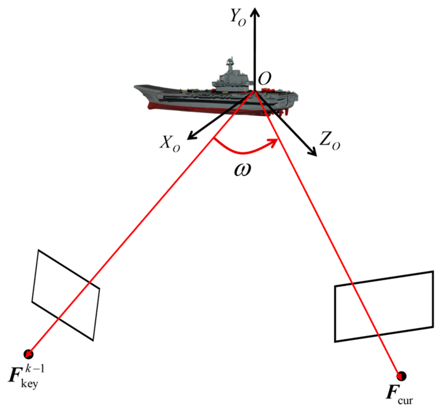
This paper adopts the geometry constraints within the monocular image sequence to handle the absence of an accurate 3D model. The accuracy of multi-view geometry constraints mainly depends on the following two critical factors: Firstly, the accuracy of 2D observations, which usually involves the precise extraction and positioning of feature points, line segments, or other geometric elements in the image, and, secondly, the magnitude of the rendezvous angle between viewpoints in the image sequence, which affects the stability and accuracy of reconstructing the 3D structure from different viewpoints. Thus, the accuracy of 2D landmark detection and the rendezvous angle of the image sequence are two crucial factors that influence the performance of the proposed method.

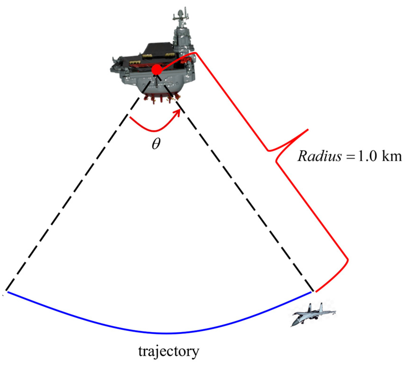
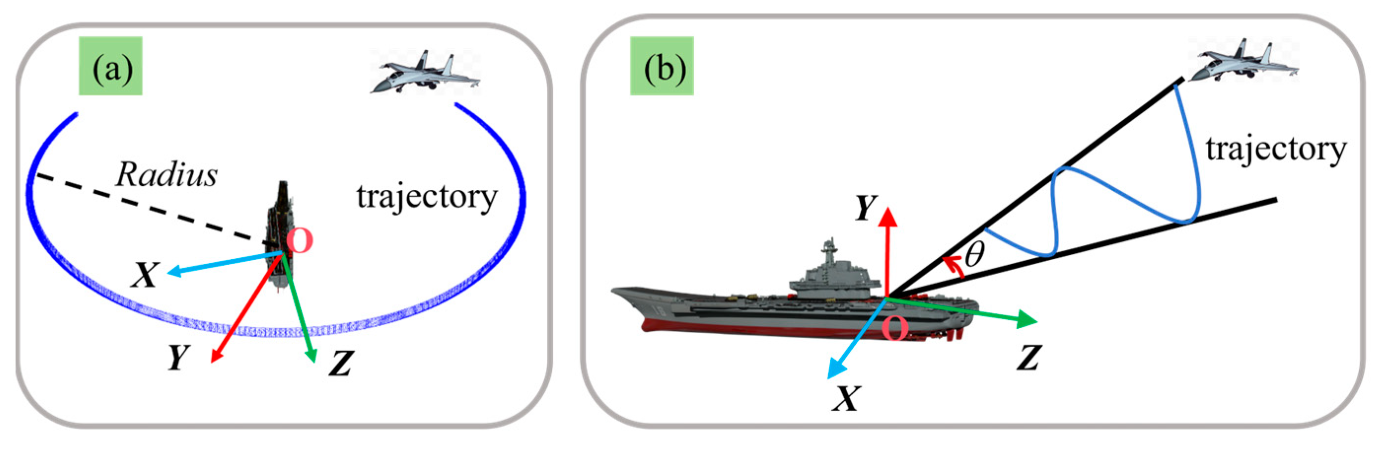
This paper takes the autonomous landing of UAVs as an example to verify the proposed method. Hence, as depicted in Figure 6, this paper simulates the UAV flying around the central axis of the stern of the ship at a distance of 1.0 km. And the simulation experiment data are generated synchronously. In Figure 6, $\theta$ represents the setting rendezvous angle. Additionally, the projection of the 3D landmarks on the image is computed based on the true poses corresponding to the simulated trajectory.

The optimization objective function presented in this paper jointly optimizes the 3D model and poses by minimizing the reprojection error. Hence, a significant 2D landmark detection error can result in the failure of the proposed method. To investigate the tolerance level of the proposed method towards landmark detection errors, this paper first selects the simulation data with $\theta ={180}^{\circ }$. 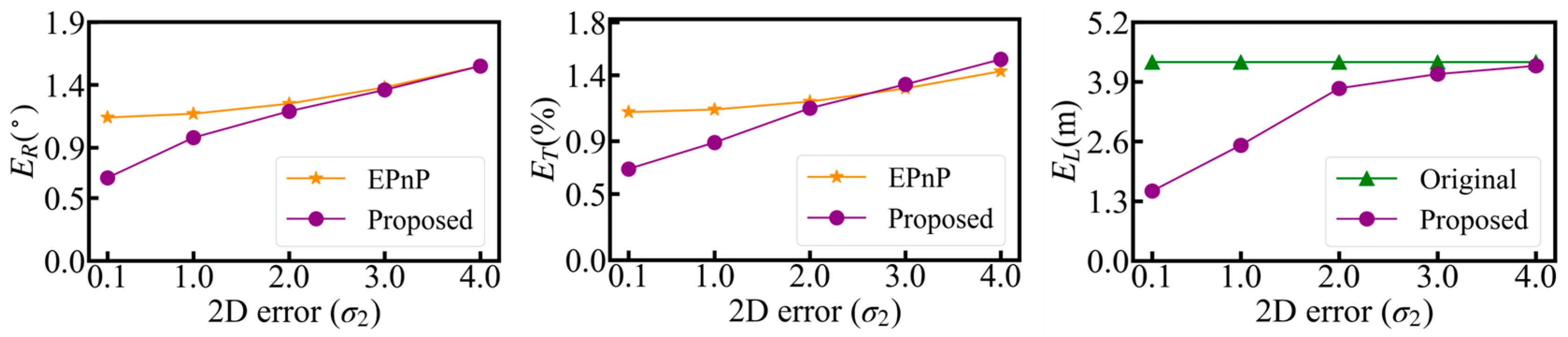Subsequently, this paper simulates 2D landmark detection errors by adding different levels of Gaussian noise $\mathcal{N}(0,{\sigma }_2)$ to 2D landmark ground truth. And different noise levels were simulated 1000 times, respectively. The average optimization outcomes of the pose and 3D model are depicted in Figure 7. In Figure 7 and the subsequent images, EPnP indicates the pose error acquired directly by resolving the PnP problem. The proposed represents the pose and 3D model error obtained through the further optimization of the proposed method. The original represents the initial 3D model error.

As depicted in Figure 7, when ${\sigma }_2$ is less than 2.0, the proposed method effectively mitigates the pose and 3D model error by leveraging the multi-view geometry constraints information and attains high-precision monocular pose estimation. However, when ${\sigma }_2$ exceeds 2.0, the optimization ability of the proposed method for the 3D model attenuates, thereby further causing the pose error of the solution to be close to or even exceed that solved by EPnP. Thus, within the established simulation application scenario, the proposed method demands that the 2D noise standard deviation ${\sigma }_2$ be less than 2.0 for the effective optimization of the 3D model and poses. In fact, the above experiments indicate that the proposed method requires the reprojection error of the 3D model to be greater than the 2D landmark error to effectively optimize the 3D model and pose.

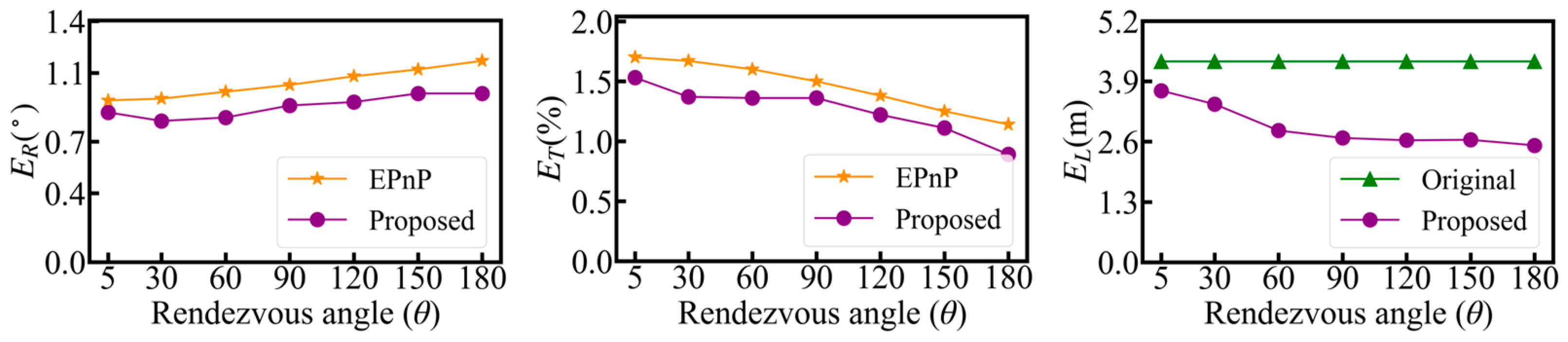
The proposed method jointly optimizes the 3D model and poses by leveraging the multi-view geometry constraints information. Hence, when the rendezvous angle is minor, it might cause insufficient geometry constraints of the observed data, thereby leading to a poorer optimization effect of the 3D model and pose. To investigate the impact of various rendezvous angles on the optimization effect of the proposed method, this paper first selects the simulation data with ${\sigma }_2=1.0$ and simulates it 1000 times. Subsequently, as depicted in Figure 6, data segments with varying rendezvous angles $\theta$ were selected from the simulation data for optimization. The average optimization outcomes of the pose and 3D model are depicted in Figure 8.

As depicted in Figure 8, when the rendezvous angle varies within the range of 5 degrees to 180 degrees, in all instances, the proposed method has mitigated the errors of the 3D model and the pose to a certain extent. However, when the rendezvous angle is 5 degrees, the optimization effect of the 3D model and the pose is insufficiently conspicuous. In actuality, the optimization outcome at this point merely holds statistical significance but lacks practical value for application. It can be observed from Figure 8 that, within the established simulation application scenario, when the rendezvous angle exceeds 30 degrees, the proposed method can largely reduce the errors of the 3D model and pose. In fact, within the optimization approach presented in this paper, a larger rendezvous angle encompasses more geometry constraint information, which is more conducive to the optimization of 3D models and poses.

Through the above experiments, it was discovered that when the accuracy of the 2D landmarks was relatively high, that is, when its error was smaller than the reprojection error of the 3D model, the proposed method exhibited excellent performance. Additionally, when the rendezvous angle between the viewpoints in the image sequence was large, the proposed method was capable of further effectively jointly optimizing the 3D model and poses.

4.3. Experiments on Synthetic Image Sequences

In this section, this paper selects synthetic image sequences to conduct an experiment. The synthetic images are produced through the target’s 3D model combined with a computer graphics engine. Specifically, this paper employs the visual simulation tool BlenderProc [51] to load the 3D CAD model of the ship. It sets the image resolution of the virtual camera to $1024\times 1024$ pixels, the focal length to 1910 pixels, the acquisition frame rate to 25 fps, and the field of view angles to 30° (horizontal) and 30° (vertical). As depicted in Figure 9, within the synthetic environments, corresponding image data are produced by establishing diverse camera trajectories. The generated synthetic image sequences are elaborated in detail below.

In Figure 9a, $Radius$ represents the flight radius parameter. The experiment detailed in Section 4.2 demonstrates that in the circular flight scenario with a radius of 1 km, the proposed method can accommodate significant landmark noise. The detection of 2D landmarks in the synthetic images is comparatively precise. Consequently, in this section, the $Radius$ in Figure 9a is set to 2.0 km to investigate the optimization in a more distant circular flight scenario. And image sequence, namely Orbit-2.0 ($Radius=2.0\mathrm{km}$) is produced. In Figure 9b, the rendezvous process of the UAV and the ships with different small rendezvous angles is simulated. And the image sequences Rendezvous-10 ($\theta ={10}^{°}$), Rendezvous-20 ($\theta ={20}^{°}$), and Rendezvous-30 ($\theta ={30}^{°}$) are generated, respectively.

This paper selects Orbit-2.0, Rendezvous-10, Rendezvous-20, and Rendezvous-30 image sequences to conduct the experiment. Additionally, existing approaches typically adopt sparse or dense 2D–3D correspondence and directly resolve PnP problems to obtain pose estimation outcomes. Consequently, this paper separately employs the current cutting-edge RTMpose and PP-TinyPose [52] approaches to detect 2D landmarks. Then, this paper contrasts the proposed method with the RTMPose-EPnP and PP-TinyPose-EPnP methods. Both the RTMPose-EPnP and PP-TinyPose-EPnP methods further solve PnP problems on the basis of landmark detection to obtain pose results.

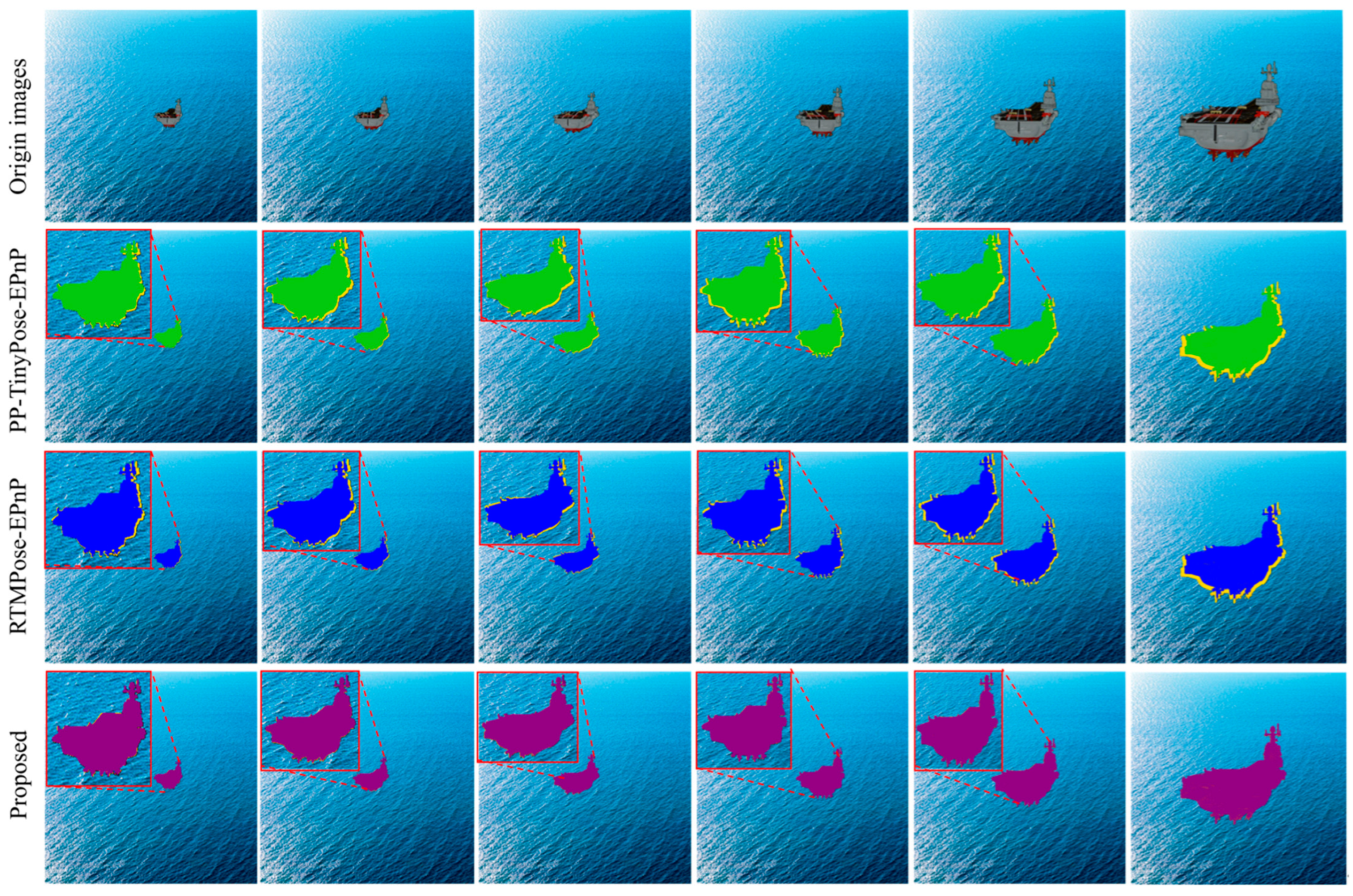
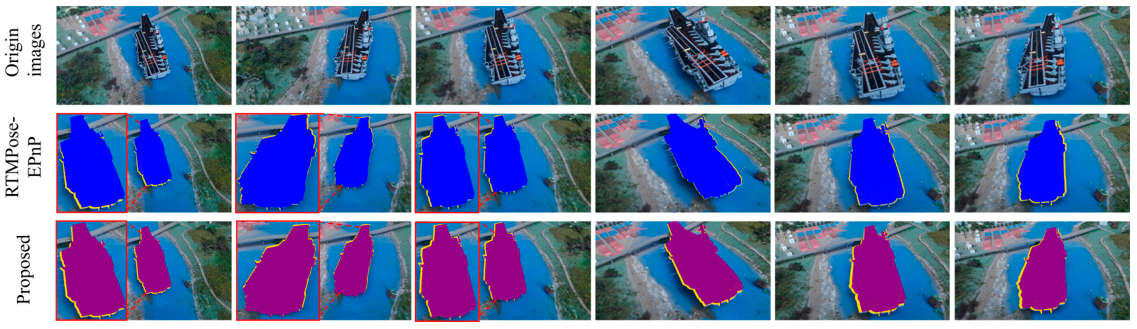
The synthetic example results of reprojection using the poses of PP-TinyPose-EPnP, RTMPose-EPnP, and the proposed method are presented in Figure 10, where the local zoomed-in results of the reprojection image are displayed in the red box at the upper left corner. And the yellow mask represents the ground truth, the green mask indicates the reprojection using the pose solved by PP-TinyPose-EPnP, the blue mask represents the reprojection using the pose solved by RTMPose-EPnP, and the purple mask corresponds to the proposed method.

As depicted in Figure 10, owing to the inaccurate target’s 3D model, the PP-TinyPose-EPnP and RTMPose-EPnP methods fail to acquire precise poses. As demonstrated in the pose reprojection outcomes of the second and third rows, the pose reprojection results based on the two comparative methods do not fully align with the genuine target area. The proposed method takes advantage of the constraint information of multi-view geometry constraints to jointly optimize the target’s 3D model and pose parameters. The experimental results presented in the fourth row of Figure 10 indicate that, by employing the proposed method, the reprojected target region conforms splendidly to the ground truth. The outcomes reveal that the proposed method can accomplish high-precision monocular pose estimation in the absence of an accurate target.

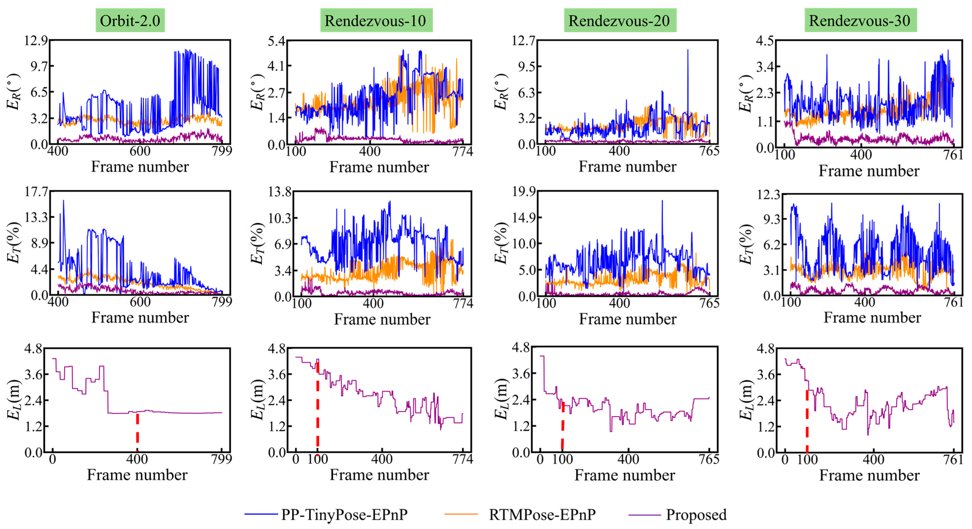
To quantitatively assess the performance of various methods in predicting pose, based on Equation (13), this paper selects a set of complete pose prediction samples from four synthetic image sequences, respectively. These samples are depicted in the first two rows of Figure 11. Additionally, the proposed method is configured to output the pose optimization results of the current frame only when the number of optimized keyframes reaches the length of the sliding window. Thus, Figure 11 presents only the optimized portion of the image sequence. In addition, the third row of Figure 11 exhibits the variation in the average error of the target’s 3D model throughout the entire optimization within the four image sequence samples. Meanwhile,

Table 2. NME results of 2D landmark detection based on RTMPose and PP-TinyPose in synthetic experiment. The minimum error is shown in bold.

Methods	Evaluation Metrics	Orbit-2.0	Rendezvous-10	Rendezvous-20	Rendezvous-30
PP-TinyPose	$\mathrm{NME}\times 100$ (%)	3.90	7.89	7.94	7.21
RTMPose	$\mathrm{NME}\times 100$ (%)	0.48	0.32	0.33	0.35

presents the average detection outcomes of 2D landmarks for PP-TinyPose and RTMPose in various synthetic image sequences.

As depicted in the first two rows of Figure 11, within four image sequence samples, as a consequence of errors in the target’s 3D model and the detected 2D landmarks, the PP-TinyPose-EPnP and RTMPose-EPnP methods fail to obtain precise poses. Especially, as depicted in Table 2, the 2D landmark error identified by PP-TinyPose is more substantial. Hence, the pose error addressed by PP-TinyPose-EPnP is conspicuously larger than that addressed by RTMPose-EPnP and the proposed method. In contrast, RTMPose has a relatively high accuracy in detecting 2D landmarks, and its detection error is less than the reprojection error of the 3D model. Hence, the proposed method utilizes multi-view geometry constraints to jointly optimize the target’s 3D model and pose, obtaining high-precision poses. As depicted in the third row of Figure 11, throughout the entire joint optimization procedure, the error of the target’s 3D model generally manifests a downward trend. Hence, the pose error achieved by resolving the PnP problem based on the optimized 3D model is reduced accordingly.

In Orbit-2.0, the long imaging distance will magnify the influence of 2D errors on the optimization. Consequently, the successful pose optimization outcomes on Orbit-2.0 suggest that the approach presented in this paper is moderately robust against 2D landmark detection errors at extended distances. As analyzed in Section 4.2, the rendezvous angles of Rendezvous-10, Rendezvous-20, and Rendezvous-30 are relatively small and unable to provide sufficient information for optimization. However, the continuous proximity between platforms serves to mitigate the influence of 2D detection errors on the proposed optimization algorithm. Hence, the proposed method still achieves favorable pose optimization results on these three sequence samples.

Figure 11 depicts the pose prediction outcomes of a solitary sample from each of the four synthetic image sequences. Subsequently,

Table 3. Results of pose estimation from four synthetic image sequences. The minimum error is shown in bold.

Image Sequences	${\mathit{E}}_{\mathit{R}}\left(\mathsf{°}\right)$			${\mathit{E}}_{\mathit{T}}\left(\mathsf{\%}\right)$
	PP-TinyPose-EPnP	RTMPose-EPnP	Proposed	PP-TinyPose-EPnP	RTMPose-EPnP	Proposed
Orbit-2.0	3.34	1.41	1.23	2.71	1.24	1.12
Rendezvous-10	1.73	1.39	0.38	4.11	2.31	0.69
Rendezvous-20	1.27	1.39	0.48	2.85	2.28	0.69
Rendezvous-30	1.73	1.40	0.47	3.78	2.27	0.71

exhibits the statistical findings of the average pose errors of all samples within the four synthetic image sequences, with the minimum error highlighted in bold.

As demonstrated in Table 3, in comparison with the PP-TinyPose-EPnP and RTMPose-EPnP approaches, the proposed method achieves the pose prediction outcomes that are closest to the ground truth in all four image sequences. Additionally, as can be observed from Table 3, due to the magnified impact of a greater distance on the 2D landmark detection error, the optimization effect of the pose in Orbit-2.0 is marginally subpar.

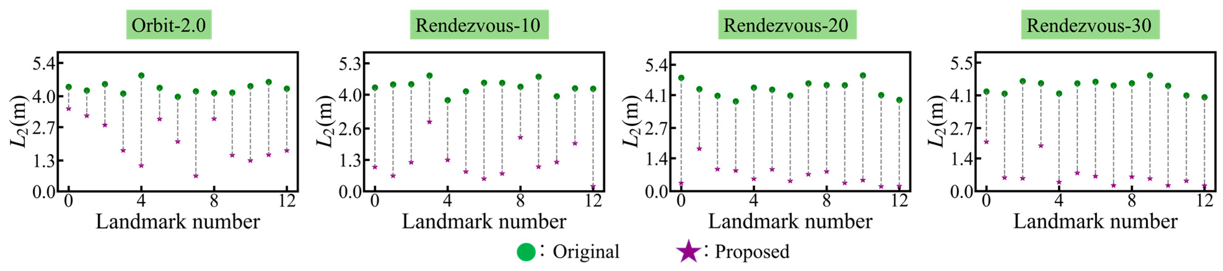
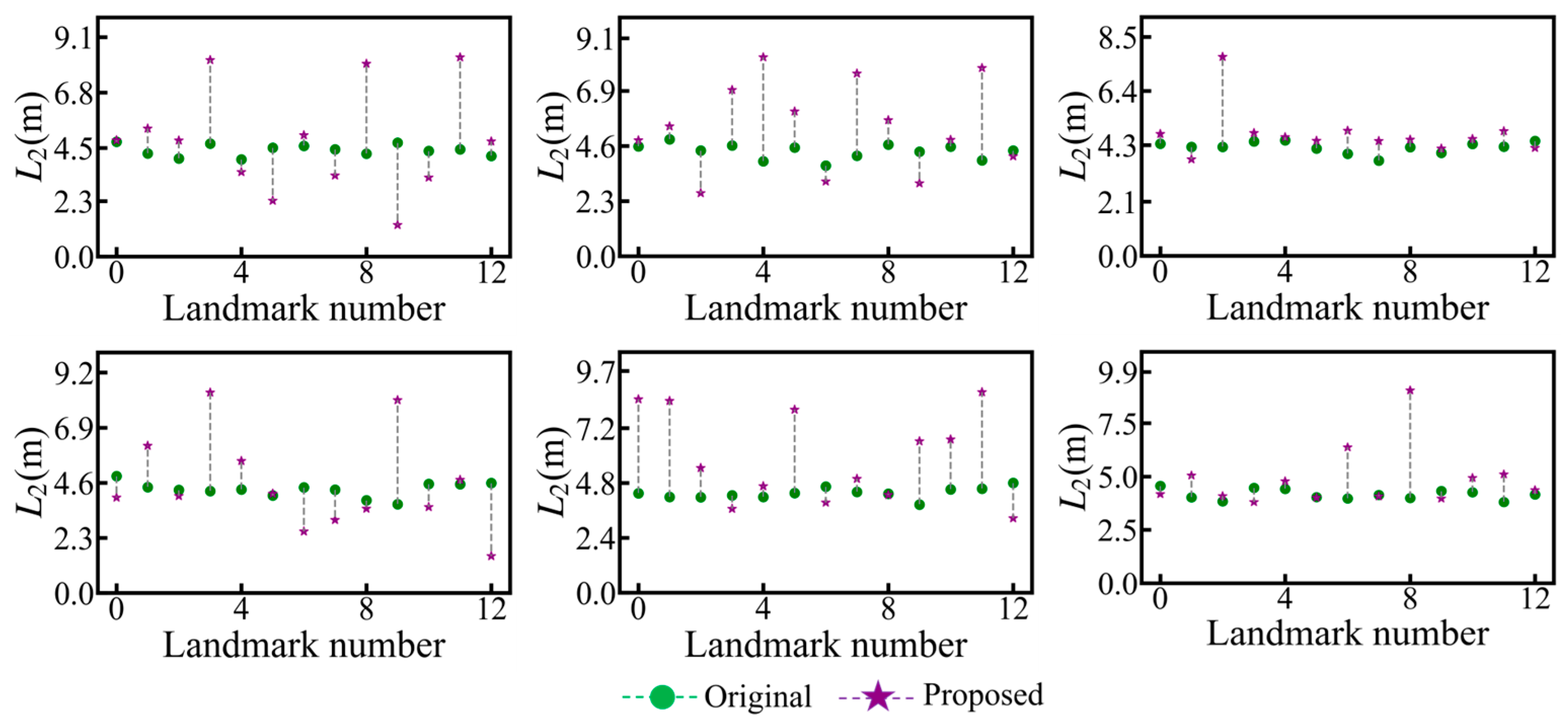
The proposed method employs multi-view geometry constraint information to jointly optimize the target’s 3D model and pose. Consequently, the optimization effect of the proposed method for the 3D model on a single sample from each of the four image sequences is presented in Figure 12. In this figure, the green dot represents the original 3D model error and the purple five-pointed star represents the optimized 3D model error. As depicted in Figure 12, the proposed method effectively decreases the overall error of the 3D model within four synthetic image sequence samples.

Figure 12 exhibits the influence of 3D model optimization in a solitary sample. Subsequently,

Table 4. The average optimization results of 3D model from four synthetic image sequences. The minimum error is shown in bold.

Image Sequences	${\mathit{E}}_{\mathit{L}}\left(\mathit{m}\right)$
	Original	Proposed
Orbit-2.0	4.35	3.16
Rendezvous-10	4.35	2.30
Rendezvous-20	4.35	2.15
Rendezvous-30	4.35	2.39

presents the statistical outcomes of the average 3D model errors of all samples within four synthetic image sequences, where the minimum error is highlighted in bold.

As depicted in Table 4, the proposed method reduces the 3D model error in all four image sequences. Furthermore, a longer imaging distance will increase the impact of 2D landmark detection errors on optimization. Therefore, the optimization effect for the 3D model in the Orbit-2.0 image sequence is relatively poor.

In addition, this paper compares the processing time of different algorithms on a single frame in

Table 5. The comparison of the average processing time of different methods on synthetic image sequences.

Method	Time (ms/Frame)
PP-TinyPose-EPnP	8.15
RTMPose-EPnP	27.15
Proposed	32.15

.

As shown in Table 5, because of the benefit of the lightweight network design, PP-TinyPose-EPnP’s average processing time on the synthetic image sequence is only about 8.15 ms/frame. Due to the addition of the optimization module, the proposed method takes a longer time than RTMPose-EpnP at about 32.5 ms/frame. However, when the camera frame rate is greater than or equal to 20 Hz, the proposed method can still meet the requirements of real-time applications.

4.4. Experiments on Real Image Sequences

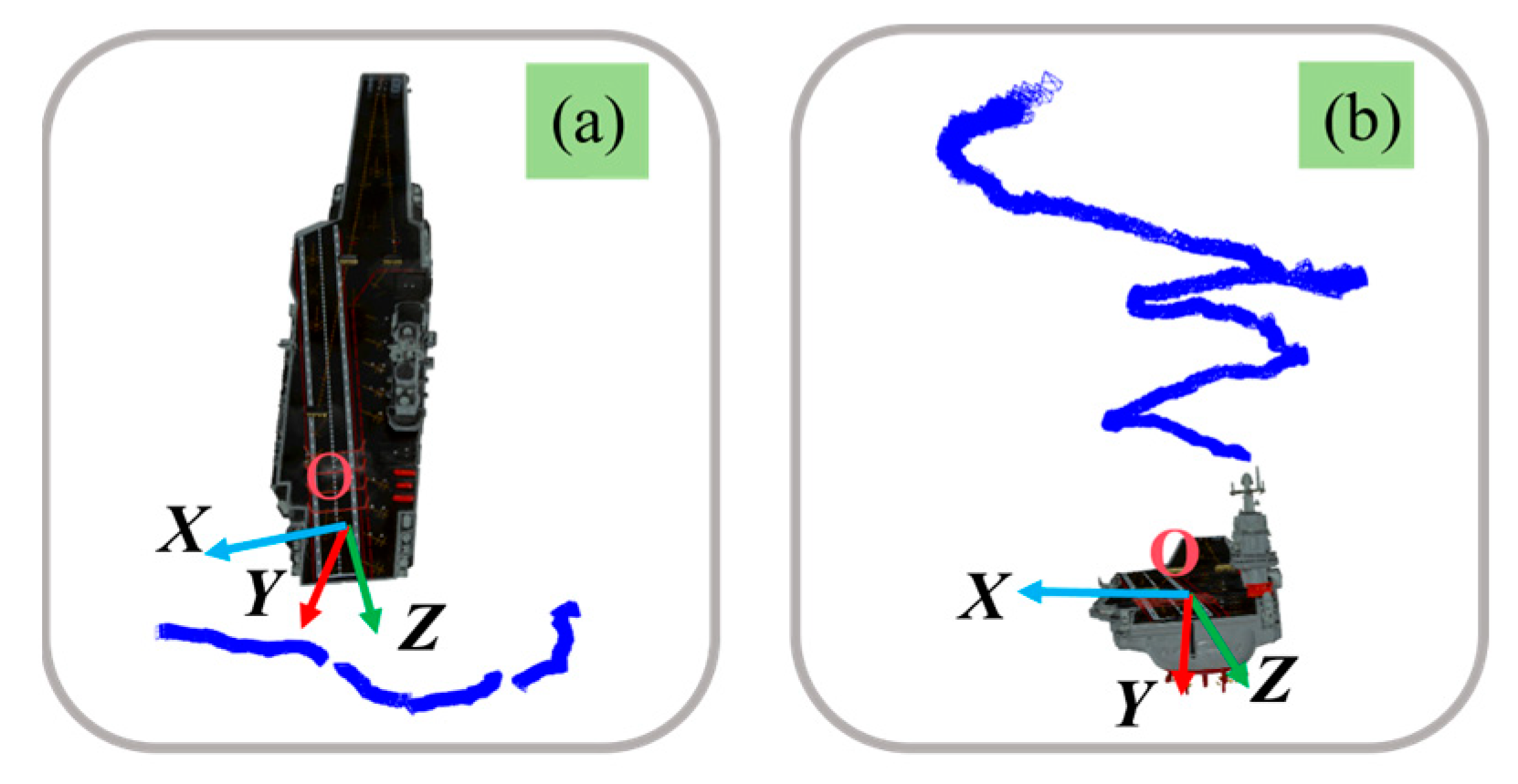
Similarly to synthetic experiments, in real experiments, this paper employs a handheld camera to simulate the scenarios where the UAV is circling around and rendezvousing with the ship. The simulation process of the UAV circling the ship at about 1 km in the real scene is presented in Figure 13a, and its corresponding image sequence is named real orbit. The simulation process of the rendezvous between the UAV and the ship in the real scene is presented in Figure 13b, and the corresponding image sequence is designated as real rendezvous. And the pose truth values for the real image sequences are obtained through manual annotation.

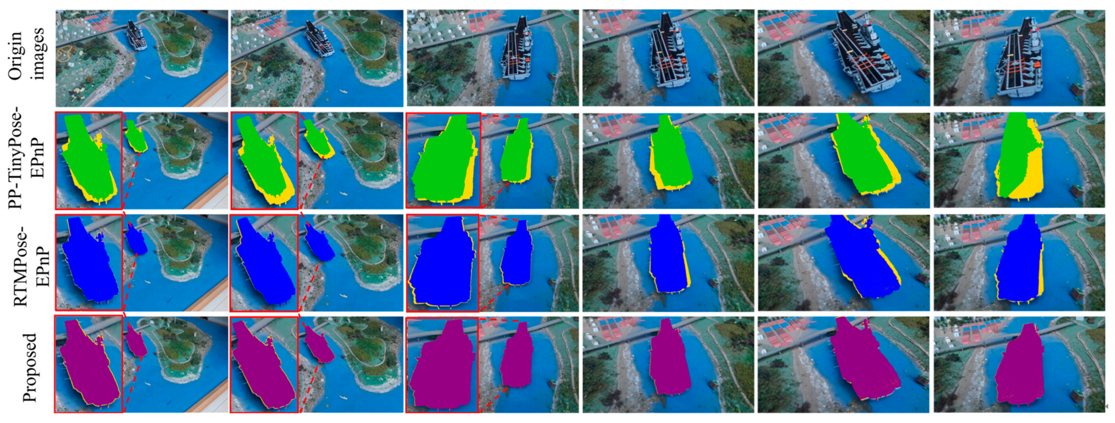
This paper selects real orbit and real rendezvous image sequences to conduct real experiments. Additionally, PP-TinyPose-EPnP and RTMPose-EPnP are also employed as comparative approaches. Similarly to Figure 10, the example results of pose reprojection of PP-TinyPose-EPnP, RTMPose-EpnP, and the proposed method on real image sequences are presented in Figure 14, where the local zoomed-in results of pose reprojection are depicted in the red box on the left. The meanings represented by the different color masks in the figure are consistent with those in Figure 10. Moreover, Table 5 presents the average detection outcomes of 2D landmarks for PP-TinyPose and RTMPose in various real image sequences.

In

Table 6. NME results of 2D landmark detection based on RTMPose and PP-TinyPose in real experiment. The minimum error is shown in bold.

Methods	Evaluation Metrics	Real Orbit	Real Rendezvous
PP-TinyPose	$\mathrm{NME}\times 100$ (%)	5.28	4.91
RTMPose	$\mathrm{NME}\times 100$ (%)	0.29	0.29

, The 2D landmark detection error of PP-TinyPose on real image sequences is significantly greater than that of RTMPose. Therefore, in Figure 14, even the pose reprojection of PP-TinyPose-EPnP exhibits severe deformation, indicating that the obtained pose results deviate significantly from the ground truth. In contrast, the accuracy of 2D landmarks detected by RTMPose generally meets the boundary conditions given in Section 4.2. Therefore, the poses obtained by RTMPose-EPnP and the proposed method are more accurate. Furthermore, as shown in the first two examples in Figure 14, due to the relatively large detection error of the 2D landmarks in the real image sequence, the subsequent optimization effect on the pose is poor.

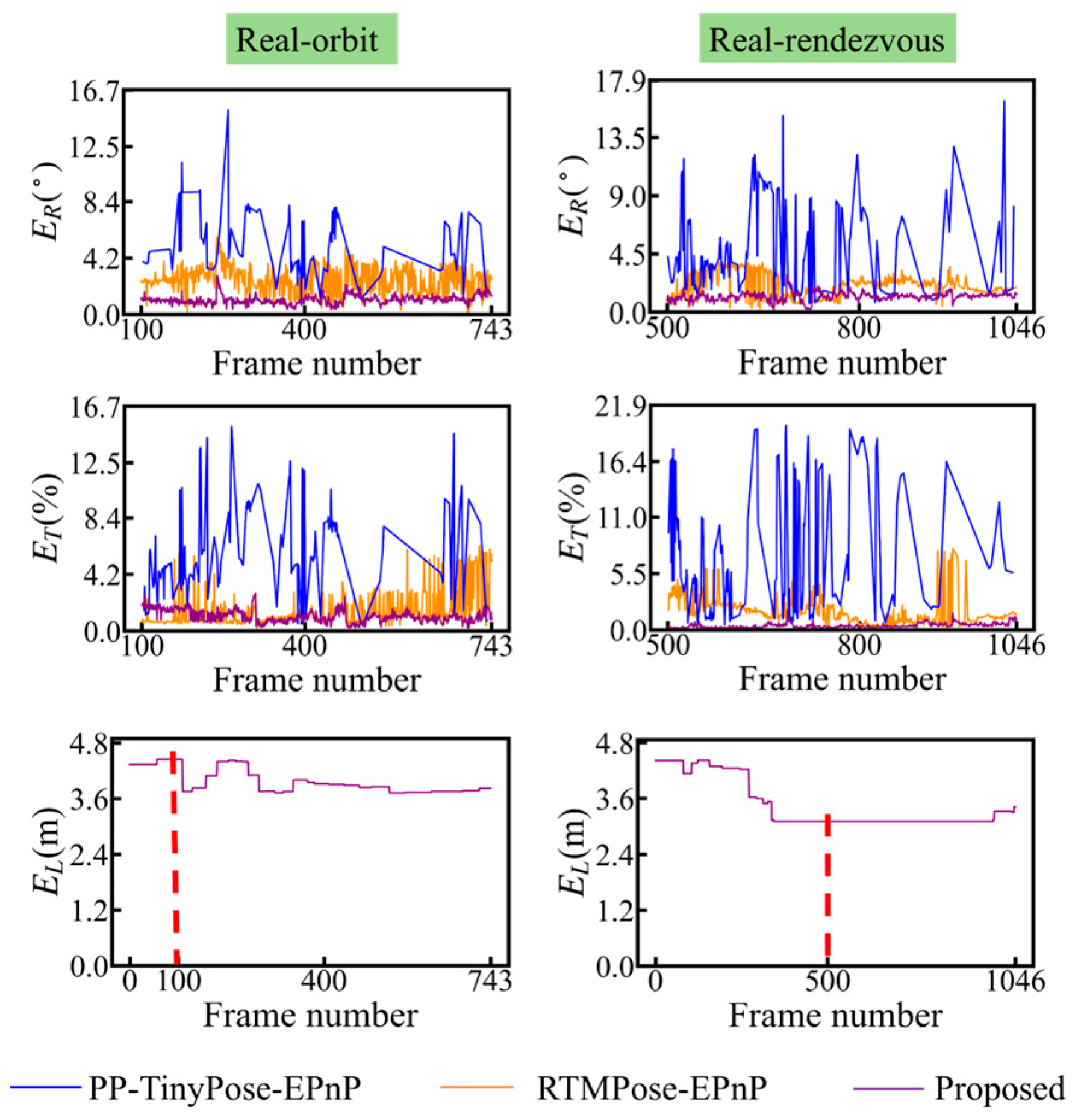
Similarly to the synthesis experiment, this paper selects a set of complete pose prediction samples from two real image sequences, respectively. These samples are depicted in the first two rows of Figure 15. In addition, the third row of Figure 15 exhibits the variation in the average error of the target’s 3D model throughout the entire optimization within the two image sequence samples.

As depicted in the initial two rows of Figure 15, the pose errors achieved by the proposed method are consistently smaller than those obtained through the PP-TinyPose-EPnP and RTMPose-EPnP methods throughout the image sequence. This is predominantly due to the fact that, as exhibited in the third row of Figure 15, the proposed method continuously diminishes the error of the 3D model during the optimization procedure, thereby reducing the pose error. However, owing to the significant 2D detection error in real images, the optimization effect of the 3D model presented in Figure 15 is not as satisfactory as that of the synthetic experiment. As a result, in Figure 15, the pose error curves of RTMPose-EPnP and the proposed method are not discriminated clearly enough. Additionally, in a few images, the pose error achieved by RTMPose-EPnP is smaller than that in the proposed method.

Figure 15 depicts the pose prediction outcomes of a solitary sample from each of the two real image sequences. Subsequently,

Table 7. Results of pose estimation from two real image sequences. The minimum error is shown in bold.

Image Sequences	${\mathit{E}}_{\mathit{R}}\left(\mathsf{°}\right)$			${\mathit{E}}_{\mathit{T}}\left(\mathsf{\%}\right)$
	PP-TinyPose-EPnP	RTMPose-EPnP	Proposed	PP-TinyPose-EPnP	RTMPose-EPnP	Proposed
Real orbit	10.82	2.24	1.45	12.78	2.19	1.34
Real rendezvous	6.69	2.30	1.23	10.44	2.69	1.33

exhibits the statistical findings of the average pose errors of all samples within the two real image sequences, with the minimum error highlighted in bold.

As demonstrated in Table 7, in comparison with the PP-TinyPose-EPnP and RTMPose-EPnP approaches, the proposed method achieves the pose prediction outcomes that are closest to the ground truth in all two image sequences.

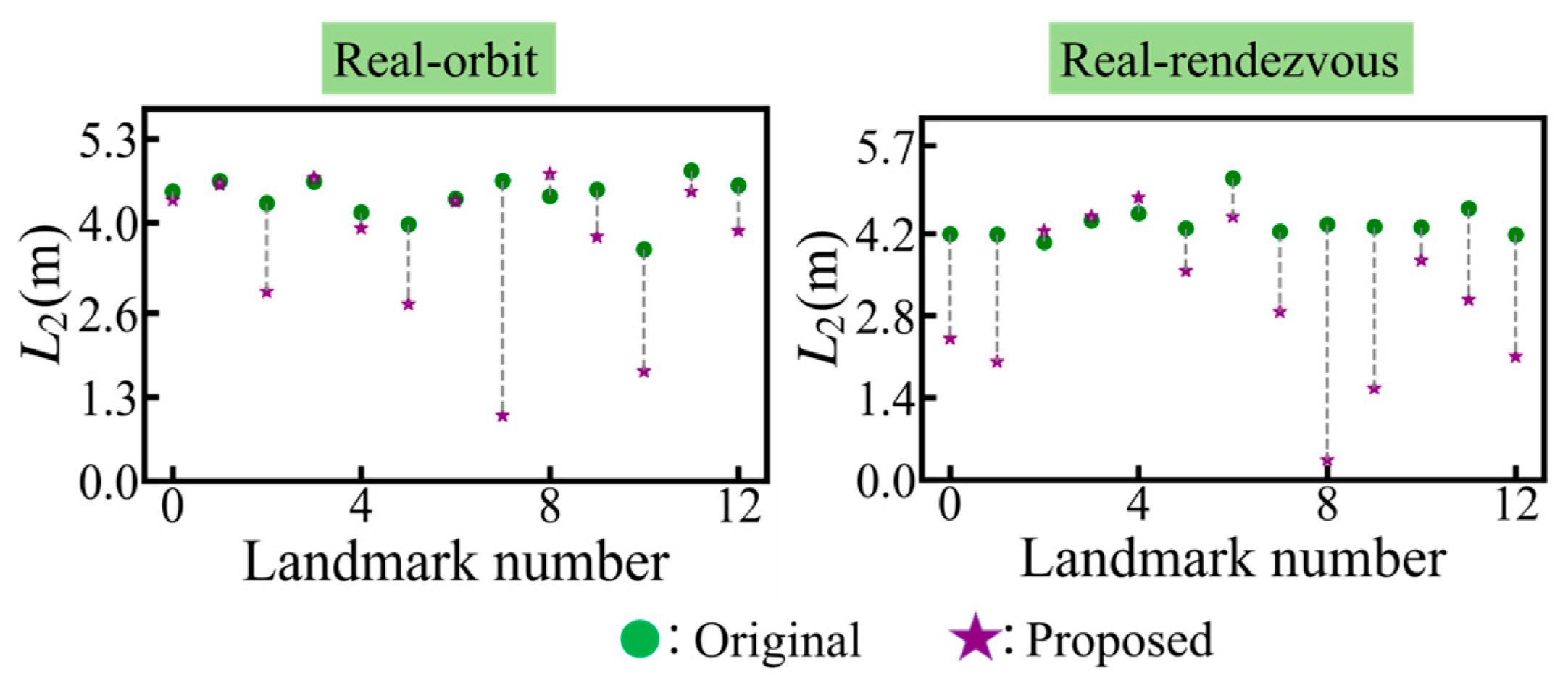
The proposed method employs multi-view geometry constraint information to jointly optimize the target’s 3D model and pose. Consequently, the optimization effect of the proposed method for the 3D model on a single sample from each of the two image sequences is presented in Figure 16. In this figure, the green dot represents the original 3D model error and the purple five-pointed star represents the optimized 3D model error.

As depicted in Figure 16, the proposed method effectively decreases the overall error of the 3D model within two real image sequence samples. However, in contrast to the synthesis experiments, in Figure 16, the errors of a few 3D landmarks further escalate after optimization. This is mainly due to the large 2D landmark detection error on the real image sequence, which is not conducive to the subsequent optimization based on minimizing the reprojection error.

Figure 16 exhibits the influence of 3D model optimization in a solitary sample. Subsequently,

Table 8. The average optimization results of 3D model from two real image sequences. The minimum error is shown in bold.

Image Sequences	${\mathit{E}}_{\mathit{L}}\left(\mathit{m}\right)$
	Original	Proposed
Real orbit	4.35	4.18
Real rendezvous	4.35	3.88

presents the statistical outcomes of the average 3D model errors of all samples within two real image sequences, where the minimum error is highlighted in bold.

As depicted in Table 8, the proposed method reduces the 3D model error in all two image sequences. Furthermore, in line with the aforementioned analysis, on account of the significant 2D detection error, the optimization effect of the 3D model in the real image sequence is restricted. For instance, in real orbit, the model error is reduced by merely approximately 4%, while in real rendezvous, the model error is decreased by approximately 10%. Therefore, high-precision 2D landmark detection is of crucial importance to the proposed method.

In addition, this paper compares the processing time of different algorithms on a single frame in

Table 9. The comparison of the average processing time of different methods on real image sequences.

Method	Time (ms/Frame)
PP-TinyPose-EPnP	9.15
RTMPose-EPnP	29.15
Proposed	36.15

.

Similarly to the statistics in synthetic experiments, in real experiments, PP-TinyPose-EPnP consumes the least amount of time. RTMPose-EPnP takes slightly longer, approximately 29.15 ms. The proposed method has the longest duration of around 36.15 ms. It can be observed that, compared to synthetic experiments, the optimization module consumes more time in real experiments. This is primarily due to the larger landmark detection errors in real image sequences, which subsequently leads to an increase in the number of iterations required by the optimization module. Additionally, inaccurate landmark detection implies larger errors in the initial pose estimation, requiring the optimization algorithm to take longer to find the correct convergence direction.

4.5. Limitation Analysis

The joint optimization outcomes in synthetic and real image sequences demonstrate that the proposed method can effectively diminish the errors in both the pose and the target’s 3D model. Nevertheless, in some samples, as a result of significant 2D landmark detection errors, the proposed approach fails to effectively optimize the pose and 3D model.

Figure 17 shows the pose optimization failure results from a real sample. Since the pose error acquired by the PP-TinyPose-EPnP approach is considerably oversized, we merely compare RTMPose-EPnP and the proposed method. Further, Figure 18 shows the multi-set failure optimization results of the target’s 3D model in real image sequences. In certain images within the real image sequence, the detection errors of 2D landmarks are significantly larger than the reprojection error of the 3D model. Consequently, as depicted in Figure 17 and Figure 18, it is challenging for the method presented in this paper to optimize the pose and 3D model by minimizing the reprojection error.

The current research of this paper primarily focuses on landmark detection under sufficient lighting and clear image conditions. And the in-depth discussions and experiments under adverse weather conditions have yet to be conducted. Consequently, the proposed method may exhibit lower robustness and accuracy in these challenging environments. This is primarily due to the fact that the algorithm learns feature representations under favorable conditions during the training process. Therefore, it lacks sufficient adaptability to the variations in image features under extreme weather conditions.

To enhance the robustness of the landmark detection algorithm under adverse weather conditions, this study will improve the proposed method in two aspects for future work. Firstly, this study introduced simulated adverse weather condition data (such as generating images with intense light, rain, snow, or fog through image processing techniques) during the training process to increase the model’s adaptability to such conditions. Secondly, this study explored the integration of other sensor data (such as infrared cameras, LiDAR, etc.) to assist in landmark detection, thereby improving detection accuracy and stability under adverse weather conditions.

5. Conclusions

Aiming at the issue of pose estimation of UAV autonomous landing missions with the absence of an accurate 3D model, this paper proposes a new monocular pose estimation method that jointly optimizes the target’s 3D model and poses. This paper represents the target’s 3D model using a set of sparse 3D landmarks. A trained neural network is used to detect the landmarks from the input image. Furthermore, the correction value of the target’s 3D model and pose are taken as parameters to be optimized. Then, the optimization objective function based on minimizing the reprojection error is established. By solving the optimization problem, the target’s 3D model and poses are optimized jointly. And, with the absence of an accurate 3D model, the high-precision pose is obtained. Moreover, a sliding window combined with a keyframe extraction strategy is also adopted in the proposed method to improve the processing speed of the algorithm. The experimental results on synthetic and real data demonstrate that the proposed method can achieve real-time and online high-precision pose estimation for the case in which the accurate 3D model is unavailable.

Despite the manifest effect of the joint 3D model and pose optimization, the proposed method still has the issue that it is not applicable to large 2D landmark detection errors. In addition, this paper does not focus on the robustness of landmark detection under adverse weather conditions. In subsequent work, this study plans to improve the adaptability of the model by incorporating data from harsh weather conditions during the training process. Additionally, it aims to explore the integration of sensors such as infrared cameras and radars to assist in landmark detection. To improve the accuracy of landmark detection, we will probe into the utilization of multi-view geometry constraint information of sequence images to further diminish 2D detection landmark errors. Additionally, in the next work, by enhancing the expression form of the parameters in the optimization equation, the joint optimization of the target’s 3D model and poses with considerable 2D noise will be deliberated.