Seal Pipeline: Enhancing Dynamic Object Detection and Tracking for Autonomous Unmanned Surface Vehicles in Maritime Environments

Abstract

This study addresses the dynamic object detection problem for Unmanned Surface Vehicles (USVs) in marine environments, which is complicated by boat tilting and camera illumination sensitivity. A novel pipeline named “Seal” is proposed to enhance detection accuracy and reliability. The approach begins with an innovative preprocessing stage that integrates data from the Inertial Measurement Unit (IMU) with LiDAR sensors to correct tilt-induced distortions in LiDAR point cloud data and reduce ripple effects around objects. The adjusted data are grouped using clustering algorithms and bounding boxes for precise object localization. Additionally, a specialized Kalman filter tailored for maritime environments mitigates object discontinuities between successive frames and addresses data sparsity caused by boat tilting. The methodology was evaluated using the VRX simulator, with experiments conducted on the Volga River using real USVs. The preprocessing effectiveness was assessed using the Root Mean Square Error (RMSE) and tracking accuracy was evaluated through detection rate metrics. The results demonstrate a 25% to 30% improvement in detection accuracy and show that the pipeline can aid industry even with sparse object representation across different frames. This study highlights the potential of integrating sensor fusion with specialized tracking for accurate dynamic object detection in maritime settings, establishing a new benchmark for USV navigation systems’ accuracy and reliability.

1. Introduction

Unmanned Surface Vehicles (USVs) have become integral to a wide array of maritime applications, including pipeline inspection, environmental monitoring, and rescue missions, thanks to their capability to autonomously execute complex tasks [1,2,3,4,5,6]. The evolution of USV autonomy aims to enhance both safety and operational efficiency in dynamic and often unpredictable water environments. However, one of the significant challenges in advancing USV autonomy is detection and tracking of dynamic objects, a task complicated by various environmental factors such as water reflection, waves, and the instability caused by USV movements in response to rolling, pitching, and yawing (RPY) motions.

These environmental factors present unique obstacles in accurately determining the position and orientation of objects relative to the USV. Water reflections can interfere with camera-based systems, while turbulent conditions can create noise in sensor data, especially with LiDARs. Moreover, objects such as bridges, boats, and other waterborne obstacles come in a wide range of shapes and sizes, further complicating navigation and detection processes. Therefore, the selection of appropriate sensors and the development of a robust detection and tracking system are critical for enabling USVs to operate safely and autonomously in these challenging environments.

The maritime industry requires reliable USVs capable of effectively navigating these dynamic waters to perform critical tasks such as inspecting pipelines and conducting rescue missions. Successful execution of these tasks depends on the accurate detection and tracking of dynamic objects, allowing USVs to navigate obstacles autonomously. Current approaches rely heavily on cameras and LiDARs, each of which faces limitations in these environments. Cameras are vulnerable to issues such as water reflections and low-light performance, while LiDAR systems often struggle with noise introduced by waves and surface reflections. Additionally, the instability of USVs due to water-induced tilt fluctuations can affect the accuracy of these sensors, leading to incomplete or inaccurate data.

This paper introduces a novel detection and tracking pipeline named the Seal Pipeline, which is designed to enhance the capabilities of USVs in dynamic maritime environments by addressing key challenges in object detection and tracking. Existing methods for object detection in USVs often rely on cameras and LiDARs, and consequently face significant limitations. Cameras are susceptible to errors caused by reflections, illumination variations, and reduced effectiveness in low-light conditions, particularly in dynamic water environments [7,8,9]. LiDARs, while providing more accurate distance measurements through time of flight (TOF) calculations, encounter challenges from water surface reflections, especially in turbulent conditions caused by waves or moving vessels. These disturbances result in noisy data, complicating the differentiation between actual objects and noise from water ripples. Additionally, tilt fluctuations of USVs due to wave motion disrupt the accuracy of LiDAR data, given the limited vertical range of such sensors. The Seal Pipeline addresses these challenges by combining innovative data preprocessing and postprocessing techniques, advanced segmentation methods, and predictive modeling to mitigate the effects of environmental noise and USV motion on sensor data. By leveraging advanced sensor fusion to integrate data from both LiDARs and cameras, the Seal Pipeline enhances the autonomy and operational effectiveness of USVs in maritime applications, providing a comprehensive solution for reliable object detection in water environments. This contribution holds the potential to significantly improve the performance of USVs in complex maritime settings, overcoming the limitations of existing detection systems.

Paper Structure

The rest of this paper is organized as follows: Section 2 presents a detailed review of related work on object detection and tracking for USVs, emphasizing the methods employed for sensor fusion and segmentation in dynamic environments; Section 3 outlines the methodology behind the development of the Seal Pipeline, explaining the innovative data preprocessing, postprocessing techniques, and sensor fusion algorithms that address the challenges of environmental noise and USV motion; Section 4 discusses the experimental setup, evaluation metrics, and results obtained from testing the Seal Pipeline, providing a detailed analysis of the performance improvements achieved; finally, Section 5 concludes with a summary of the key contributions and highlights potential directions for future work.

2. Related Work

Accurate detection and tracking of objects in maritime environments is essential for the safe and efficient operation of USVs. However, achieving reliable performance in dynamic water conditions remains a significant challenge. This section reviews the relevant literature, focusing on camera-based detection, LiDAR-based approaches, sensor fusion techniques, and challenges in navigable region detection. Additionally, we draw comparisons with similar challenges in other domains, such as spaceborne Synthetic Aperture Radar (SAR) and underwater vehicles, highlighting how different techniques address analogous issues. Through this review, we underscore the limitations of current methods and identify areas where this study makes novel contributions.

2.1. Camera-Based Detection Methods

Cameras are frequently used in USVs for obstacle detection, often employing stereo vision systems to estimate depth and identify objects. Huntsberger et al. [10] and Martins et al. [11] explored the use of stereo vision to detect obstacles in marine environments. While effective in calm conditions, these methods struggle in dynamic environments characterized by high waves and water ripples. Reflections from the water surface and varying illumination conditions further complicate accurate detection.

Recent studies such as that of Zhan et al. [9] have attempted to improve detection by employing approximate semantic segmentation for water surface detection using stereo cameras. While this approach reduces false positives, it suffers from inaccurate depth estimation and remains sensitive to weather and lighting conditions. These limitations underscore the need for additional sensors or enhanced processing to ensure reliable detection in a wider range of environmental conditions.

Similar challenges have been addressed in spaceborne Synthetic Aperture Radar (SAR) systems, which face range ambiguity issues when detecting targets across varying terrain. The work of [12] introduced blind source separation techniques to mitigate these ambiguities, highlighting the relevance of advanced signal processing techniques in overcoming environmental interference.

2.2. LiDAR-Based Detection Approaches

LiDAR technology has been widely adopted for detecting and tracking objects in open water environments due to its ability to generate precise point cloud data [13,14,15]. Han et al. [13] utilized LiDAR for object segmentation, employing the Inscribed Angle Variance (IAV) technique combined with the Gaussian-means (G-means) algorithm to improve detection accuracy. However, while effective for identifying stationary structures such as bridges and towers, this method does not account for dynamic objects such as boats that are commonly encountered in water environments.

Jeong et al. [16] addressed this limitation by proposing a method to detect in-water obstacles using 3D LiDAR data converted into 2D spherical projections. While this technique improves real-time object segmentation in aquatic environments, projecting 3D data into 2D results in some loss of information, limiting its effectiveness in tracking dynamic objects.

Autonomous underwater vehicles (AUVs) also face detection and tracking challenges in environments with limited visibility, as demonstrated by [17]. Vision-based tracking methods for AUVs share similarities with LiDAR-based detection in USVs, particularly in dealing with dynamic and noisy environments. In both cases, the need for robust real-time processing and sensor fusion techniques is crucial to enhance object detection and tracking accuracy.

2.3. Data Fusion Methods

The fusion of multiple sensors, particularly cameras and LiDARs, has been explored to overcome the limitations of individual sensing systems. Wang et al. [18] developed a data fusion approach that combines 3D point cloud data with visual information to improve the accuracy of object detection in marine environments. This method significantly reduces the impact of water reflections and ripples, leading to improved accuracy over traditional detection systems.

Thompson [19] emphasized the importance of LiDAR and camera sensor fusion for object detection and navigation in maritime environments, with classification being performed by a Support Vector Machine (SVM) [20]. However, this approach is designed for prior known classes, which is not efficient for detecting and tracking static and dynamic unknown objects.

In spaceborne SAR systems, sensor fusion methods have also been employed to improve detection reliability under adverse conditions. The work of [12] leveraged the fusion of radar signals with blind source separation to enhance target identification amid ambiguous data, drawing a parallel to the challenges faced in fusing camera and LiDAR data in marine environments.

2.4. Challenges in Navigable Region Detection

Yao et al. [21] introduced a method for segmenting navigable regions in river environments using minimum convex polygons. While effective in reducing noise from LiDAR point cloud data, this approach was designed for narrow rivers and does not generalize well to broader and more dynamic marine environments.

Studies such as [22] have incorporated deep learning and Kalman filters to improve object tracking and navigable area detection. However, these methods focus primarily on static obstacles such as riverbanks and bridges, leaving a gap in addressing dynamic objects.

Similar challenges are encountered in underwater environments, where AUVs must navigate and detect obstacles in murky waters. Vision-based tracking methods such as those explored by [17] demonstrate the need for advanced preprocessing and fusion techniques to overcome noisy input data, much as in in the case of USVs dealing with water surface reflections and dynamic obstacles.

In summary, while existing approaches to object detection and tracking in marine environments have made considerable progress, they remain limited by their sensitivity to environmental conditions and the dynamic behavior of water surfaces. The current paper addresses these gaps by proposing the Seal Pipeline, a comprehensive solution that combines sensor fusion, robust preprocessing and postprocessing techniques, and advanced tracking algorithms to handle both static and dynamic objects in challenging water environments. The proposed framework is designed to significantly enhance the operational reliability of USVs, offering a novel contribution to the field of maritime autonomy.

3. Methodology

This article addresses the challenge of tilt fluctuations commonly experienced by non-terrestrial autonomous vehicles such as drones and boats. Our methodology consists of multiple steps: a preprocessing step that eliminates tilt fluctuations and noise; object detection using a clustering algorithm, to which bounding boxes are appended for subsequent tracking; and a Kalman filter employed for precise object tracking across various subsequent frames. This paper underscores a comprehensive procedure for enhancing object detection precision for dynamic objects in a maritime environment, Figure 1.

3.1. Data Collection and Sensor Integration

This methodology section details the system and sensors utilized for data collection, focusing on the integration of IMU and LiDAR sensors to correct tilt-induced distortions and reduce noise without delving into experimental specifics. This framework incorporates two primary data streams: LiDAR-generated point clouds and rotational data captured by the IMU from the boat. These two data streams are fused to mitigate the effects of tilt and dynamic fluctuations caused by water movement, ensuring precise and stable spatial data collection. LiDAR provides high-resolution spatial information for object detection, while the IMU captures the orientation data needed to correct for the boat’s roll, pitch, and yaw.

Each sensor is modeled mathematically to describe how measurements relate to the system state. The IMU model is expressed as

$${\mathbf{z}}_{\mathrm{IMU}}=h_{\mathrm{IMU}}\left(\mathbf{x}\right)+{\mathbf{n}}_{\mathrm{IMU}},$$

(1)

where ${\mathbf{z}}_{\mathrm{IMU}}$ represents the IMU measurements, $h_{\mathrm{IMU}}\left(\mathbf{x}\right)$ is a nonlinear function linking the state to the IMU output, and ${\mathbf{n}}_{\mathrm{IMU}}$ denotes the measurement noise.

Similarly, the LiDAR sensor is modeled as

$${\mathbf{z}}_{\mathrm{LiDAR}}=h_{\mathrm{LiDAR}}\left(\mathbf{x}\right)+{\mathbf{n}}_{\mathrm{LiDAR}},$$

(2)

where ${\mathbf{z}}_{\mathrm{LiDAR}}$ represents the LiDAR measurements, $h_{\mathrm{LiDAR}}\left(\mathbf{x}\right)$ is the function mapping the state to LiDAR observations, and ${\mathbf{n}}_{\mathrm{LiDAR}}$ accounts for noise.

To effectively fuse the IMU and LiDAR data, it is essential to align the timestamps between these sensors to ensure synchronization of the measurements. Timestamp misalignment is addressed through interpolation of IMU data to match LiDAR timestamps, defined as follows:

$${\mathbf{z}}_{\mathrm{IMU},\mathrm{aligned}}=I({\mathbf{z}}_{\mathrm{IMU}},t_{\mathrm{LiDAR}})$$

(3)

where I denotes the interpolation function that adjusts the IMU data to the corresponding LiDAR measurement timestamps.

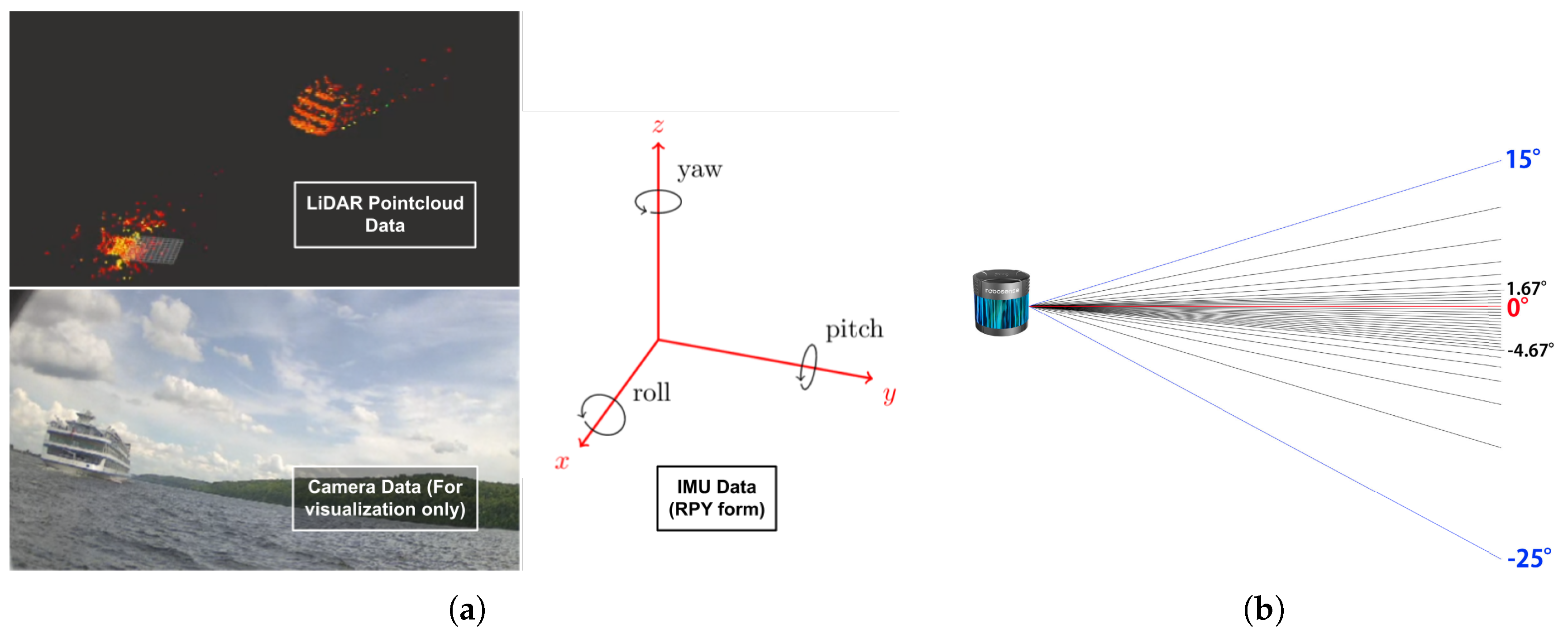
Figure 2a illustrates data acquired from the LiDAR, camera, and IMU sensors. It is noteworthy that the camera-captured images serve solely for visualization and debugging purposes, and do not contribute to the data processing pipeline.

IMU data, represented as quaternions, are converted to Roll ($\varphi$), Pitch ($\theta$), and Yaw ($\psi$) angles for a more intuitive representation of the boat’s orientation with respect to the $\mathbf{X}$, $\mathbf{Y}$, and $\mathbf{Z}$ axes. These angles are derived using the formulas shown below.

$$\varphi =arctan\left({\displaystyle \frac{2(q_4{q}_1+q_2{q}_3)}{1-2(q_1^2+q_2^2)}}\right)\left(\mathrm{Roll}\right)$$

(4)

$$\theta =arcsin\left(2(q_2{q}_4-q_1{q}_3)\right)\left(\mathrm{Pitch}\right)$$

(5)

$$\psi =arctan\left({\displaystyle \frac{2(q_4{q}_3+q_1{q}_2)}{1-2(q_2^2+q_3^2)}}\right)\left(\mathrm{Yaw}\right)$$

(6)

These transformations allow us to account for the boat’s tilt and provide the necessary corrections to the point cloud data based on the boat’s orientation relative to the $\mathbf{X}$, $\mathbf{Y}$, and $\mathbf{Z}$ axes.

For enhanced analysis and calibration, we also consider the angular velocities (${\dot{\varphi }}_a$, ${\dot{\theta }}_a$, ${\dot{\psi }}_a$) and linear accelerations ($a_x$, $a_y$, $a_z$) derived from the IMU data. The angular velocities are calculated as follows:

$${\dot{\varphi }}_a={\omega }_x+sin\left(\varphi \right)tan\left(\theta \right){\omega }_y+cos\left(\varphi \right)tan\left(\theta \right){\omega }_z$$

(7)

$${\dot{\theta }}_a=cos\left(\varphi \right){\omega }_y-sin\left(\varphi \right){\omega }_z$$

(8)

$${\dot{\psi }}_a={\displaystyle \frac{sin\left(\varphi \right)}{cos\left(\theta \right)}}{\omega }_y+{\displaystyle \frac{cos\left(\varphi \right)}{cos\left(\theta \right)}}{\omega }_z$$

(9)

where ${\omega }_x$, ${\omega }_y$, and ${\omega }_z$ are the angular velocity components measured by the IMU.

To transform the linear accelerations from the body frame to the inertial frame, we employ the rotation matrix R derived from the quaternion [23,24,25,26]. The transformation is described by

$$\left[\begin{array}{c}{a}_{x_{inertial}}\\ a_{y_{inertial}}\\ a_{z_{inertial}}\end{array}\right]=R·\left[\begin{array}{c}{a}_x\\ a_y\\ a_z\end{array}\right],$$

(10)

where the rotation matrix R is provided by

$$R=\left[\begin{array}{ccc}1-2(q_2^2+q_3^2)& 2(q_1{q}_2-q_4{q}_3)& 2(q_1{q}_3+q_4{q}_2)\\ 2(q_1{q}_2+q_4{q}_3)& 1-2(q_1^2+q_3^2)& 2(q_2{q}_3-q_4{q}_1)\\ 2(q_1{q}_3-q_4{q}_2)& 2(q_2{q}_3+q_4{q}_1)& 1-2(q_1^2+q_2^2)\end{array}\right].$$

(11)

To enhance the accuracy of our sensor data interpretation, we integrate Kalman filtering techniques. This approach helps to mitigate noise and improve the estimation of the boat’s state by combining the LiDAR and IMU data streams. The state estimation vector $\mathbf{x}$ and the process model can be represented as follows:

$${\mathbf{x}}_{k+1}=\mathbf{A}{\mathbf{x}}_k+\mathbf{B}{\mathbf{u}}_k+{\mathbf{w}}_k$$

(12)

where $\mathbf{A}$ is the state transition matrix, $\mathbf{B}$ is the control input matrix, ${\mathbf{u}}_k$ is the control vector, and ${\mathbf{w}}_k$ represents the process noise. The initial state vector ${\mathbf{x}}_0$ is defined as follows:

$${\mathbf{x}}_0={\widehat{\mathbf{x}}}_0$$

(13)

where ${\widehat{\mathbf{x}}}_0$ is the initial estimate of the state vector. This estimate is often derived from prior data or domain knowledge about the system.

The measurement update equation is provided by

$${\mathbf{z}}_k=\mathbf{H}{\mathbf{x}}_k+{\mathbf{v}}_k,$$

(14)

where $\mathbf{H}$ is the measurement matrix and ${\mathbf{v}}_k$ is the measurement noise.

To achieve optimal sensor fusion, a weighting scheme is applied based on the relative noise characteristics of each sensor. The measurement covariance matrices ${\mathbf{R}}_{\mathrm{IMU}}$ and ${\mathbf{R}}_{\mathrm{LiDAR}}$ quantify the uncertainty in IMU and LiDAR data, respectively. The Kalman gain $\mathbf{K}$, which determines the contribution of each sensor to the state update, is computed as follows:

$$\mathbf{K}={\mathbf{P}}_{k|k-1}{\mathbf{H}}^T{(\mathbf{H}{\mathbf{P}}_{k|k-1}{\mathbf{H}}^T+{\mathbf{R}}_k)}^{-1},$$

(15)

where ${\mathbf{P}}_{k|k-1}$ is the prior error covariance and ${\mathbf{R}}_k$ combines the measurement noise from both IMU and LiDAR.

By implementing this fusion algorithm, we are able to combine the spatial accuracy of LiDAR with the orientation precision of the IMU, correcting for tilt and dynamic fluctuations caused by the water. The resulting data fusion enhances the precision and stability of the spatial measurements.

3.2. Preprocessing

Preprocessing is a vital step in enhancing the quality of point cloud data. It involves correcting for orientation errors, reducing noise, and stabilizing the data to accurately reflect the environment. This section outlines the mathematical methods used for these tasks. To align the point cloud data with the world coordinate system, we need to account for the boat’s orientation relative to the LiDAR sensor. This orientation correction involves applying a rotation matrix R derived from te roll ($\varphi$), pitch ($\theta$), and yaw ($\psi$) angles obtained from the IMU.

The transformation of a point ${\mathbf{P}}_L={[x_L,y_L,z_L,1]}^T$ from the LiDAR frame to the world frame ${\mathbf{P}}_W$ is provided by

$${\mathbf{P}}_W=R(\varphi ,\theta ,\psi )·{\mathbf{P}}_L,$$

(16)

where the rotation matrix $R(\varphi ,\theta ,\psi )$ is defined as

$$R(\varphi ,\theta ,\psi )=R_z\left(\psi \right)·R_y\left(\theta \right)·R_x\left(\varphi \right)$$

(17)

and the individual rotation matrices are

$$R_x\left(\varphi \right)=\left[\begin{array}{ccc}1& 0& 0\\ 0& cos\left(\varphi \right)& -sin\left(\varphi \right)\\ 0& sin\left(\varphi \right)& cos\left(\varphi \right)\end{array}\right],$$

(18)

$$R_y\left(\theta \right)=\left[\begin{array}{ccc}cos\left(\theta \right)& 0& sin\left(\theta \right)\\ 0& 1& 0\\ -sin\left(\theta \right)& 0& cos\left(\theta \right)\end{array}\right],$$

(19)

$$R_z\left(\psi \right)=\left[\begin{array}{ccc}cos\left(\psi \right)& -sin\left(\psi \right)& 0\\ sin\left(\psi \right)& cos\left(\psi \right)& 0\\ 0& 0& 1\end{array}\right].$$

(20)

Following orientation correction, the next task is noise reduction, which is crucial for eliminating artifacts such as ripples caused by water. We implement a height-based filtering approach to remove points below a specified threshold.

The filtered point cloud ${\mathbf{P}}_W^{filtered}$ is provided by

$${\mathbf{P}}_W^{filtered}=\left\{{\mathbf{P}}_W\mid z_W\ge z_{threshold}\right\}.$$

(21)

Here, $z_{threshold}$ is typically set to zero or a small positive value to exclude points representing the water surface.

Point cloud stabilization is performed to compensate for dynamic changes due to the boat’s movement, ensuring that the data reflect a stable reference frame. This is achieved by applying a homogeneous transformation matrix $H_{4\times 4}$ derived from the IMU data.

The stabilized point cloud ${\mathbf{P}}_W$ is obtained by

$${\mathbf{P}}_W=H_{4\times 4}^{-1}·{\mathbf{P}}_L.$$

(22)

The homogeneous transformation matrix $H_{4\times 4}$ is

$$H_{4\times 4}=\left[\begin{array}{cc}{R}_{3\times 3}& \mathbf{t}\\ 0& 1\end{array}\right],$$

(23)

where $R_{3\times 3}$ is the $3\times 3$ rotation matrix representing orientation correction and $\mathbf{t}$ is the translation vector, which is typically zero if no translation is applied.

To clarify the covariance matrices used in our preprocessing, Equation (16) transforms point cloud data from the LiDAR frame (${\mathbf{P}}_L$) to the world frame (${\mathbf{P}}_W$) using the rotation matrix $R(\varphi ,\theta ,\psi )$. Equation (22) stabilizes the point cloud data using the inverse of the transformation matrix $H_{4\times 4}$.

The covariance matrices are defined as follows:

• ${\mathbf{P}}_W$: Uncertainty in the point cloud after orientation correction.
• ${\mathbf{P}}_L$: Uncertainty in the raw LiDAR data before stabilization.

The accuracy of object detection and tracking in LiDAR systems depends heavily on the quality of the point cloud data. However, raw point cloud data often contain noise and orientation distortions due to environmental factors and the movement of the boat. To address these issues, a preprocessing step is applied to the data, which includes correcting orientation errors, removing noise, and stabilizing the data to ensure reliable object detection.

3.3. Clustering Algorithm

Clustering is a vital step in maritime object detection where environmental factors such as water movement and sensor noise add complexity. This manuscript focuses on Euclidean distance-based (k-means) clustering and DBSCAN algorithms due to their robustness in handling spatial data and noise tolerance, which is essential in dynamic maritime environments. However, it is acknowledged that other clustering techniques, such as hierarchical clustering or Gaussian mixture models (GMM), could also be considered depending on the dataset’s structure and application.

The primary rationale for selecting these clustering methods is that k-means clustering is computationally efficient for large datasets, while DBSCAN is particularly well suited to nonlinear shapes and can handle noise, which is a common challenge in maritime environments. Although hierarchical clustering and GMM are viable options, k-means and DBSCAN were prioritized for their computational simplicity and noise-handling capabilities, which are well suited to real-time processing and environmental variability.

3.3.1. Euclidean Distance-Based Clustering

Euclidean distance-based clustering approaches [27] such as k-means group datapoints based on their proximity. The Euclidean distance between points ${\mathbf{p}}_i=(x_i,y_i,z_i)$ and ${\mathbf{p}}_j=(x_j,y_j,z_j)$ is provided by

$$d({\mathbf{p}}_i,{\mathbf{p}}_j)=\sqrt{{(x_i-x_j)}^2+{(y_i-y_j)}^2+{(z_i-z_j)}^2}.$$

(24)

In k-means clustering, the objective is to minimize the within-cluster sum of squares (WCSS):

$$\mathrm{WCSS}=\sum _{k=1}^K\sum _{{\mathbf{p}}_i\in C_k}{\parallel {\mathbf{p}}_i-{\mathit{\mu }}_k\parallel }^2$$

(25)

where $C_k$ represents the k-th cluster, ${\mathbf{p}}_i$ is a point in cluster $C_k$, and ${\mathit{\mu }}_k$ is the centroid of cluster $C_k$. The centroid ${\mathit{\mu }}_k$ is updated iteratively as follows:

$${\mathit{\mu }}_k={\displaystyle \frac{1}{|C_k|}}\sum _{{\mathbf{p}}_i\in C_k}{\mathbf{p}}_i$$

(26)

while the convergence criterion for k-means is

$$\Delta ={\displaystyle \frac{1}{N}}\sum _{k=1}^K\sum _{{\mathbf{p}}_i\in C_k}{∥{\mathbf{p}}_i-{\mathit{\mu }}_k^{(t+1)}-{\mathit{\mu }}_k^{\left(t\right)}∥}^2,$$

(27)

where N is the total number of points and t denotes the iteration number.

K-means clustering, as shown in Algorithm 1, is particularly useful in maritime environments due to its efficiency in handling large volumes of data and its ability to cluster objects based on spatial proximity. However, it is sensitive to noise, which is why DBSCAN is introduced as a complementary approach.    

Algorithm 1: K-means clustering
	Input: Data points $\left\{{\mathbf{p}}_i\right\}$, Number of clusters K
	Output: Cluster centroids $\left\{{\mathit{\mu }}_k\right\}$, Cluster assignments
1:	Initialize centroids $\left\{{\mathit{\mu }}_k\right\}$ randomly
2:	repeat
3:	for each data point ${\mathbf{p}}_i$ do
4:		Assign ${\mathbf{p}}_i$ to the nearest centroid ${\mathit{\mu }}_k$
5:	end
6:	for each cluster $C_k$ do
7:		Update centroid ${\mathit{\mu }}_k$ using (26)
8:	end
9:	Evaluate convergence using (27)

3.3.2. DBSCAN Algorithm

The Density-Based Spatial Clustering of Applications with Noise (DBSCAN) algorithm [28] clusters data based on density as shown in Algorithm 2. Its key parameters include the maximum distance $ϵ$ and minimum number of points MinPts required to form a dense region.

A point ${\mathbf{p}}_i$ is classified as a core point if

$$\left|\right\{{\mathbf{p}}_j\mid d({\mathbf{p}}_i,{\mathbf{p}}_j)\le ϵ\left\}\right|\ge \mathrm{MinPts}.$$

(28)

Clusters are defined starting from core points as follows:

$$C_k=\bigcup _{{\mathbf{p}}_i\in C_k}\left\{{\mathbf{p}}_j\mid \mathrm{density}\text{-}\mathrm{reachable}\mathrm{from}{\mathbf{p}}_i\right\}.$$

(29)

A point $p_j$ is density-reachable from a core point $p_j$ if and only if: $p_j$ is density-reachable from $p_i$ if and only if

$$\left\{\begin{array}{c}{\mathbf{p}}_i\mathrm{is}\mathrm{a}\mathrm{core}\mathrm{point},\hfill \\ d({\mathbf{p}}_i,{\mathbf{p}}_j)\le ϵ,\hfill \end{array}\right.$$

(30)

where $d({\mathbf{p}}_i,{\mathbf{p}}_j)$ denotes the Euclidean distance between points ${\mathbf{p}}_i$ and ${\mathbf{p}}_j$ and where $ϵ$ is the predefined distance threshold. Thus, a cluster $C_k$ includes all points ${\mathbf{p}}_j$ within the $ϵ$-neighborhood of any core point ${\mathbf{p}}_i$ in $C_k$.

The distance matrix used in the DBSCAN algorithm can be formalized as follows:

$$D_{ij}=\left\{\begin{array}{cc}d({\mathbf{p}}_i,{\mathbf{p}}_j)\hfill & \mathrm{if}d({\mathbf{p}}_i,{\mathbf{p}}_j)\le ϵ\hfill \\ \infty \hfill & \mathrm{otherwise}\hfill \end{array}\right.$$

(31)

In this matrix, $d({\mathbf{p}}_i,{\mathbf{p}}_j)$ represents the Euclidean distance between points ${\mathbf{p}}_i$ and ${\mathbf{p}}_j$. If this distance exceeds the threshold $ϵ$, then the distance is set to ∞, indicating that the points are not density-reachable from each other.

Algorithm 2: DBSCAN clustering
	Input: Data points $\left\{{\mathbf{p}}_i\right\}$, $ϵ$, MinPts
	Output: Clusters and noise
1:	for each point ${\mathbf{p}}_i$ do
2:		if ${\mathbf{p}}_i$ is not yet visited then
3:			Mark ${\mathbf{p}}_i$ as visited
4:			if ${\mathbf{p}}_i$ is a core point then
5:				Create a new cluster
6:				ExpandCluster (Algorithm 3)(${\mathbf{p}}_i$, cluster)
7:			end
8:			else
9:				Mark ${\mathbf{p}}_i$ as noise
10:			end
11:		end
12:	end

Algorithm 3: ExpandCluster Subroutine

DBSCAN was chosen over alternatives such as hierarchical clustering and GMM because it can efficiently cluster noisy data without the need for prior knowledge of the number of clusters, which can vary in real-world maritime applications. Additionally, hierarchical clustering is computationally more expensive, while GMM assumes a Gaussian distribution that may not fit the irregularities of maritime object data.

3.3.3. Advanced Considerations

For enhanced clustering performance [29], several advanced techniques and mathematical formulations are employed.

Variations of DBSCAN

• OPTICS (Ordering Points To Identify the Clustering Structure):
  The OPTICS algorithm [30] produces an ordering of points based on their reachability distances. The reachability distance between points ${\mathbf{p}}_i$ and ${\mathbf{p}}_j$ is defined as follows:

  $$\mathrm{ReachDist}({\mathbf{p}}_i,{\mathbf{p}}_j)=max\left(\mathrm{CoreDist}\left({\mathbf{p}}_i\right),d({\mathbf{p}}_i,{\mathbf{p}}_j)\right)$$

  (32)

  where the core distance $\mathrm{CoreDist}\left({\mathbf{p}}_i\right)$ is

  $$\begin{array}{cc}\hfill \mathrm{CoreDist}\left({\mathbf{p}}_i\right)& =min\left\{d({\mathbf{p}}_i,{\mathbf{p}}_j)\mid \left|\left\{{\mathbf{p}}_j\mid d({\mathbf{p}}_i,{\mathbf{p}}_j)\le ϵ\right\}\right|\ge \mathrm{MinPts}\right\}.\hfill \end{array}$$

  (33)
• HDBSCAN (Hierarchical DBSCAN):
  HDBSCAN extends DBSCAN by introducing hierarchical clustering [31,32,33]. The core distance for HDBSCAN is calculated as follows:

  $${\mathrm{CoreDist}}_{HDBSCAN}\left({\mathbf{p}}_i\right)={\displaystyle \frac{1}{\left|\mathrm{neighbors}\right|}}\sum _{{\mathbf{p}}_j\in \mathrm{neighbors}}d({\mathbf{p}}_i,{\mathbf{p}}_j)$$

  (34)

  where neighbors refers to the set of points within $ϵ$ distance from ${\mathbf{p}}_i$.

Mahalanobis Distance for Clustering

The Mahalanobis distance accounts for the correlation between variables:

$$d_M({\mathbf{p}}_i,{\mathbf{p}}_j)=\sqrt{{({\mathbf{p}}_i-{\mathbf{p}}_j)}^{\top }{\mathbf{S}}^{-1}({\mathbf{p}}_i-{\mathbf{p}}_j)}$$

(35)

where $\mathbf{S}$ is the covariance matrix. This distance metric adjusts for the shape of the data distribution. Spectral clustering involves computing the Laplacian matrix

$$\mathbf{L}=\mathbf{D}-\mathbf{W},$$

(36)

where $\mathbf{D}$ is the degree matrix and $\mathbf{W}$ is the weight matrix. The eigenvalues of $\mathbf{L}$ are used to partition the data into clusters.

The normalized Laplacian matrix is provided by

$${\mathbf{L}}_n=\mathbf{I}-{\mathbf{D}}^{-1/2}\mathbf{L}{\mathbf{D}}^{-1/2},$$

(37)

where $\mathbf{I}$ is the identity matrix.

By integrating these advanced mathematical techniques and clustering methodologies, the ability of the algorithm to accurately segment and identify clusters in complex datasets is significantly enhanced. Further performance analysis and evaluation results are discussed in Section 4.

3.4. Bounding Boxes for Objects

To provide a comprehensive overview of the spatial dimensions of identified clusters, we encapsulate each cluster using an oriented bounding box. This method provides a succinct representation of the cluster’s spatial extent and orientation, as illustrated in Figure 3. The bounding box is oriented along the principal axes of the cluster, ensuring that it is as compact as possible.

3.4.1. Principal Component Analysis and Bounding Box Construction

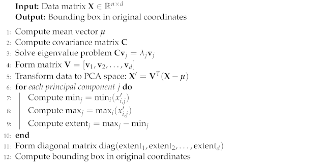
The process of constructing the bounding box involves Principal Component Analysis (PCA) [34,35,36,37] to determine the principal axes of the point cloud, which enables us to compute the minimal bounding box that encloses the cluster. Let $\mathbf{X}={[{\mathbf{x}}_1,{\mathbf{x}}_2,\dots ,{\mathbf{x}}_n]}^T\in {\mathbb{R}}^{n\times d}$ represent the matrix of n datapoints, where each ${\mathbf{x}}_i\in {\mathbb{R}}^d$ is a point in d-dimensional space. The mean vector $\mathit{\mu }\in {\mathbb{R}}^d$ is provided by

$$\mathit{\mu }={\displaystyle \frac{1}{n}}\sum _{i=1}^n{\mathbf{x}}_i,$$

(38)

while the covariance matrix $\mathbf{C}\in {\mathbb{R}}^{d\times d}$ is computed as follows:

$$\mathbf{C}={\displaystyle \frac{1}{n}}\sum _{i=1}^n({\mathbf{x}}_i-\mathit{\mu }){({\mathbf{x}}_i-\mathit{\mu })}^T.$$

(39)

PCA involves solving the eigenvalue problem for the covariance matrix

$$\mathbf{C}{\mathbf{v}}_j={\lambda }_j{\mathbf{v}}_j\mathrm{for}j=1,2,\dots ,d,$$

(40)

where ${\mathbf{v}}_j$ are the eigenvectors and ${\lambda }_j$ are the corresponding eigenvalues. The eigenvectors form an orthonormal basis for the principal directions, and the eigenvalues quantify the variance along these directions. To align the bounding box with the principal directions, we transform the point cloud into the PCA space using the orthogonal matrix $\mathbf{V}=[{\mathbf{v}}_1,{\mathbf{v}}_2,\dots ,{\mathbf{v}}_d]$:

$${\mathbf{X}}^{\prime }={\mathbf{V}}^T(\mathbf{X}-\mathit{\mu })$$

(41)

where ${\mathbf{X}}^{\prime }$ represents the point cloud in the PCA coordinate system. The coordinates of each point ${\mathbf{x}}_i^{\prime }$ are provided by

$${\mathbf{x}}_i^{\prime }={\mathbf{V}}^T({\mathbf{x}}_i-\mathit{\mu }).$$

(42)

In the PCA space, the minimal bounding box is an axis-aligned box. The extent of the bounding box along each principal component is determined by

$${\min }_j=\underset{i}{min}\left(x_{i,j}^{\prime }\right),$$

(43)

$${\max }_j=\underset{i}{max}\left(x_{i,j}^{\prime }\right).$$

(44)

The length of the bounding box along the j-th principal axis is

$${\mathrm{extent}}_j={\max }_j-{\min }_j.$$

(45)

The bounding box dimensions in the PCA space are transformed back to the original coordinate system. The bounding box in the original space is characterized by

$$\mathrm{Bounding}\mathrm{Box}=\mathbf{V}\mathrm{diag}({\mathrm{extent}}_1,{\mathrm{extent}}_2,\dots ,{\mathrm{extent}}_d){\mathbf{V}}^T,$$

(46)

where $\mathrm{diag}({\mathrm{extent}}_1,{\mathrm{extent}}_2,\dots ,{\mathrm{extent}}_d)$ is a diagonal matrix containing the extent of the bounding box along each principal component axis.

3.4.2. Optimization for Minimum Bounding Box Volume

To ensure that the bounding box is minimal, we formulate an optimization problem. The goal is to minimize the volume of the bounding box, defined as

$$V=\prod _{j=1}^d{\mathrm{extent}}_j.$$

(47)

The bounding box must contain all of the points in the cluster. Thus, the optimization problem is constrained by the following requirement:

$${\mathbf{e}}_j^T({\mathbf{x}}_i-\mathit{\mu })\ge {\mathrm{extent}}_j\mathrm{for}\mathrm{all}i$$

(48)

where ${\mathbf{e}}_j$ is the unit vector in the j-th direction.

To achieve this, we solve a quadratic programming problem with the objective function

$$\mathrm{Minimize}V=\prod _{j=1}^d\left(\underset{i}{max}\left({\mathbf{M}}_j^T{\mathbf{e}}_j\right)-\underset{i}{min}\left({\mathbf{M}}_j^T{\mathbf{e}}_j\right)\right),$$

(49)

subject to the constraints ensuring that the bounding box encloses all datapoints. This formulation can be efficiently solved using standard quadratic programming techniques. The Compute oriented bounding box algorithm is shown in Algorithm 4.

Algorithm 4: Compute oriented bounding box

3.5. Hungarian Matching Algorithm

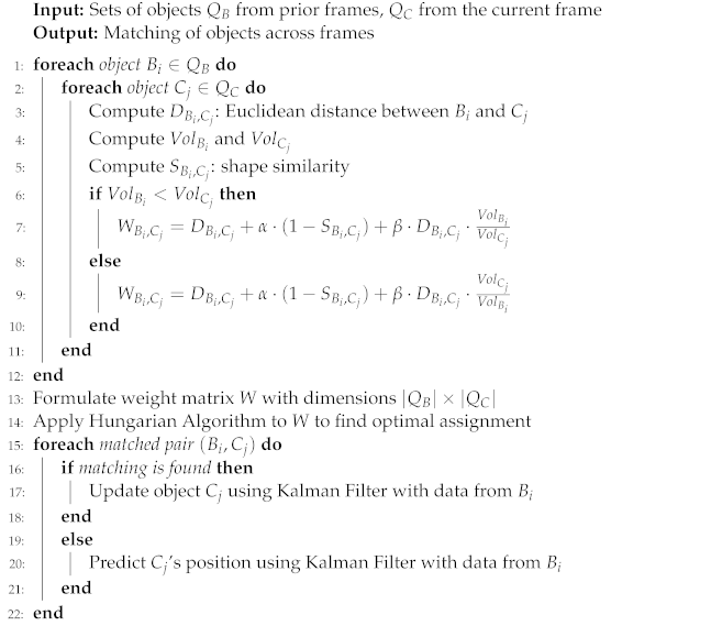
Due to the movement of the boat, a discontinuity problem arises. As shown in Figure 2b, the LiDAR has a vertical range of about −25° to 15°, meaning that objects outside this range will not have data representations from the LiDAR. Although the −25° to 15° range is sufficient to capture most objects, discontinuity appears when the boat tilts, causing the LiDAR’s horizontal line (0°) to tilt as well. Consequently, the same object may not be detected across consecutive frames. This results in objects having different numbers of points between frames, or even no points in certain frames, making it impractical to rely solely on clustering algorithms. Thus, we need to track objects to ensure that when point cloud data are missing for any given frame, we can fill the gap using data from prior frames. Here, the Hungarian Matching Algorithm (HM) [38,39,40] is utilized to match objects detected in prior frames with those in the current frame.

The matched data (from prior frames and the current frame) for the same object serve as input for the Kalman filter [41,42,43], which enhances the object’s measurements (position, orientation, dimensions). If an object in the prior frame does not match any object in the current frame, the Kalman filter algorithm predicts the object’s position in the current frame based on prior frame data.

The Hungarian Algorithm matches objects from prior frames with objects in the current frame, framing this as an assignment problem where we have n objects from prior frames and m objects from the current frame.

Assume that we have three objects from prior frames and four objects from the current frame. To achieve our goal, we establish a weight matrix with dimensions $3\times 4$, where the rows represent objects from the prior frame and the columns represent objects from the current frame, as shown in Equation (50).

$$W=\left[\begin{array}{cccc}{W}_{B1,C1}& W_{B1,C2}& W_{B1,C3}& W_{B1,C4}\\ W_{B2,C1}& W_{B2,C2}& W_{B2,C3}& W_{B2,C4}\\ W_{B3,C1}& W_{B3,C2}& W_{B3,C3}& W_{B3,C4}\end{array}\right]$$

(50)

Note: The size of W varies depending on the number of objects in the objects bank and the number of objects in the current frame’s objects array. Equation (50) uses a $3\times 4$ matrix for demonstration.

$B_i$ represents the ith object from the prior frames’ objects bank $Q_B$.

$C_j$ represents the jth object from the current frame’s objects array $Q_C$.

These weights represent the relationship between objects in prior frames and objects in the current frame. Each weight in this matrix indicates the similarity between each pair of objects; the smaller the weight, the higher the similarity and the greater the probability of a match. These weights are derived from the distance between the two objects and the ratio of their point counts, as shown in Equation (51):

$$W_{B_i,C_j}=D_{B_i,C_j}+D_{B_i,C_j}·\left\{\begin{array}{cc}{\displaystyle \frac{Vo{l}_{B_i}}{Vo{l}_{C_j}}}\hfill & \mathrm{if}Vo{l}_{B_i}<Vo{l}_{C_j}\hfill \\ {\displaystyle \frac{Vo{l}_{C_j}}{Vo{l}_{B_i}}}\hfill & \mathrm{if}Vo{l}_{B_i}\ge Vo{l}_{C_j}\hfill \end{array}\right.$$

(51)

where:

$D_{B_i,C_j}$ is the Euclidean distance between objects $B_i$ and $C_j$.

$Vo{l}_{B_i}$ is the volume of object $B_i$ from the prior frames’ list $Q_B$.

$Vo{l}_{C_j}$ is the volume of object $C_j$ from the current frame’s list $Q_C$.

Next, the W matrix shown in Equation (50) is fed into the Hungarian Algorithm to assign objects from prior frames to objects in the current frame.

To further refine the weight calculation, we incorporate more advanced mathematical models.

Let $P_{B_i}$ and $P_{C_j}$ be the sets of points belonging to objects $B_i$ and $C_j$, respectively. We define the point set distance $D_{P_{B_i},P_{C_j}}$ as the average Euclidean distance between points in $P_{B_i}$ and their nearest neighbors in $P_{C_j}$:

$$D_{P_{B_i},P_{C_j}}={\displaystyle \frac{1}{|P_{B_i}|}}\sum _{p\in P_{B_i}}\underset{q\in P_{C_j}}{min}\parallel p-q\parallel$$

(52)

where $\parallel p-q\parallel$ is the Euclidean distance between points p and q.

Additionally, we incorporate the shape similarity $S_{B_i,C_j}$ which measures the similarity of the point distribution of objects $B_i$ and $C_j$. This can be quantified using the overlap ratio of their convex hulls:

$$S_{B_i,C_j}={\displaystyle \frac{\mathrm{Area}(H_{B_i}\cap H_{C_j})}{min(\mathrm{Area}\left(H_{B_i}\right),\mathrm{Area}\left(H_{C_j}\right))}}$$

(53)

where $H_{B_i}$ and $H_{C_j}$ are the convex hulls of $P_{B_i}$ and $P_{C_j}$, respectively.

Thus, the weight $W_{B_i,C_j}$ can be refined as follows:

$$W_{B_i,C_j}=D_{P_{B_i},P_{C_j}}+\alpha ·(1-S_{B_i,C_j})+\beta ·\left\{\begin{array}{cc}{\displaystyle \frac{Vo{l}_{B_i}}{Vo{l}_{C_j}}}\hfill & \mathrm{if}Vo{l}_{B_i}<Vo{l}_{C_j}\hfill \\ {\displaystyle \frac{Vo{l}_{C_j}}{Vo{l}_{B_i}}}\hfill & \mathrm{if}Vo{l}_{B_i}\ge Vo{l}_{C_j}\hfill \end{array}\right.$$

(54)

where $\alpha$ and $\beta$ are weighting factors that respectively balance the contributions of shape similarity and volume ratio.

Finally, the refined W matrix is fed into the Hungarian Algorithm to assign objects from the prior frames to objects in the current frame, ensuring robust object tracking and reducing the discontinuity caused by the boat’s tilting motion.

While the Hungarian Algorithm is effective for object tracking, there are several limitations that should be discussed. First, in scenarios with high object density, the algorithm may struggle to differentiate between multiple objects with similar characteristics. This is particularly problematic in cluttered environments, where overlapping or closely spaced objects can result in ambiguous matches. In such cases, incorporating additional object descriptors such as texture or color information (if available) could improve performance.

Another limitation is the computational complexity of the Hungarian Algorithm, which is $O\left(n^3\right)$ for an $n\times n$ assignment problem. This can become a bottleneck as the number of objects increases, especially in real-time applications where the algorithm must operate within strict time constraints. For larger datasets, alternative approaches with lower complexity, such as the Jonker–Volgenant algorithm [44] or auction algorithms [45], may provide more efficient solutions.

Moreover, the algorithm’s reliance on geometric and volumetric data may result in incorrect matches in cases where objects have similar volumes and shapes. In such scenarios, integrating machine learning models trained on object-specific features or temporal information (e.g., motion trajectories) could improve matching accuracy.

In conclusion, while the Hungarian Matching Algorithm, see Algorithm 5, offers a solid foundation for object tracking, its performance may degrade in high-density and cluttered environments or when objects share similar features. Exploring more advanced matching techniques and integrating alternative data sources can help mitigate these challenges.

Algorithm 5: Hungarian matching algorithm for object tracking

3.6. Kalman Filter Object Tracking

A Kalman filter is employed to track objects detected in consecutive LiDAR frames while accounting for object dynamics and reducing the discontinuity caused by the boat’s movement. The state vector $\mathbf{x}$ encompasses the object’s position, orientation, and dimensions along with their rates of change.

Kalman State Vector:

$${\mathbf{x}}_{12\times 1}=\left[\begin{array}{c}X\\ Y\\ \theta \\ L\\ W\\ H\\ \dot{X}\\ \dot{Y}\\ \dot{\theta }\\ \dot{L}\\ \dot{W}\\ \dot{H}\end{array}\right]=\left[\begin{array}{c}\mathrm{X}\mathrm{coordinates}\mathrm{of}\mathrm{the}\mathrm{object}\\ \mathrm{Y}\mathrm{coordinates}\mathrm{of}\mathrm{the}\mathrm{object}\\ \mathrm{Orientation}\mathrm{of}\mathrm{the}\mathrm{object}\\ \mathrm{Length}\mathrm{of}\mathrm{the}\mathrm{object}\mathrm{Bounding}\mathrm{Box}\\ \mathrm{Width}\mathrm{of}\mathrm{the}\mathrm{object}\mathrm{Bounding}\mathrm{Box}\\ \mathrm{Height}\mathrm{of}\mathrm{the}\mathrm{object}\mathrm{Bounding}\mathrm{Box}\\ \mathrm{Object}\mathrm{Velocity}\mathrm{in}\mathrm{X}\mathrm{direction}\\ \mathrm{Object}\mathrm{Velocity}\mathrm{in}\mathrm{Y}\mathrm{direction}\\ \mathrm{Object}\mathrm{Angular}\mathrm{Velocity}\\ \mathrm{Length}\mathrm{change}\mathrm{rate}\mathrm{in}\mathrm{X}\mathrm{direction}\\ \mathrm{Width}\mathrm{change}\mathrm{rate}\mathrm{in}\mathrm{Y}\mathrm{direction}\\ \mathrm{Height}\mathrm{change}\mathrm{rate}\mathrm{in}\mathrm{Z}\mathrm{direction}\end{array}\right]$$

Kalman State Variables:

$${\mathbf{P}}_{12\times 12}={\mathbf{I}}_{12\times 12}$$

$${\mathbf{R}}_{6\times 6}=0.04·{\mathbf{I}}_{6\times 6}$$

$${\mathbf{Q}}_{12\times 12}=0.01·{\mathbf{I}}_{12\times 12}$$

$${\mathbf{H}}_{6\times 12}=\left[\begin{array}{cc}{\mathbf{I}}_{6\times 6}& {\mathbf{0}}_{6\times 6}\end{array}\right]$$

$${\mathbf{A}}_{12\times 12}={\mathbf{I}}_{12\times 12}\mathrm{where}{\mathbf{A}}_{(1,7)}={\mathbf{A}}_{(1,8)}={\mathbf{A}}_{(1,9)}=\delta t$$

For more details about the Kalman filter, refer to [46].

Kalman Filter Parameter Tuning

In dynamic and noisy environments such as marine settings, precise tuning of the Kalman filter parameters is crucial for accurate object tracking. The process of tuning these parameters was carried out by iteratively adjusting the noise covariance matrices $\mathbf{Q}$ and $\mathbf{R}$ to minimize the tracking error.

• Process Noise Covariance ($\mathbf{Q}$): This matrix controls how much uncertainty we allow in the system model. Given the inherent unpredictability of object dynamics in maritime environments (e.g., waves, vessel motion), a lower value (0.01) was chosen for $\mathbf{Q}$ to reflect relatively slow changes in the object’s motion.
• Measurement Noise Covariance ($\mathbf{R}$): The value of $\mathbf{R}$ (0.04) was selected based on empirical observations of LiDAR sensor accuracy in marine environments, considering that the measurement noise can be significant due to water reflections and surface disturbances.
• State Covariance ($\mathbf{P}$): The initial state covariance matrix $\mathbf{P}$ was set to the identity matrix to indicate equal uncertainty in all state variables before receiving observations.

For tuning the filter, certain assumptions about the marine environment and sensor data were made:

• Linear Motion Assumption: The Kalman filter assumes linear motion for tracked objects, which simplifies the computation but may not always hold true in highly dynamic scenarios. The filter’s linear state transition matrix $\mathbf{A}$ was adjusted to account for constant velocity and small object rotations.
• Gaussian Noise Assumption: The process and measurement noise were both assumed to be Gaussian-distributed, which is a standard assumption in Kalman filters but may not fully capture the complexities of noisy LiDAR data in maritime settings. Non-Gaussian noise, such as random spikes from wave reflections, was handled using gating techniques during object association.

The Kalman filter was chosen for its simplicity and computational efficiency. However, several alternative filtering methods were considered:

• Extended Kalman Filter (EKF): While the EKF has better ability to handle nonlinear motion models, its increased computational complexity was not justified by the relatively small gain in accuracy for this specific application.
• Particle Filter: Particle filters offer robust performance in highly nonlinear and non-Gaussian environments; however, these advantages come at the cost of significant computational overhead. Given the real-time requirements of the tracking system, a Kalman filter was deemed more suitable.
• Unscented Kalman Filter (UKF): The UKF was also considered for its improved ability to handle nonlinearities compared to the standard Kalman filter. However, the application of the basic Kalman filter with tuned noise parameters proved sufficient for the relatively predictable motion of objects in the test scenario.

We denote any kind of list as Q; for instance, a list of objects is denoted as $Q_{\mathrm{obj}}$ and a single object from the list is denoted as $q_{\mathrm{obj}}$.

We have the following three lists:

• $Q_B$: The bank of objects list, containing output objects of the clustering algorithm from the prior frames.
• $Q_C$: The current objects list, containing output objects of the clustering algorithm from the current frame.
• $Q_P$: The predicted objects list, containing objects that appeared in older frames but do not appear in the current frame (to be predicted in the current frame).

To track objects and enhance the output, we use Algorithm 6, where we have one of three cases for each object.

Algorithm 6: Tracking filter

3.7. Seal Pipeline

In this section, we describe the Seal Pipeline and its capabilities for maritime object detection.

Our work adopts a multimodal sensing approach by combining LiDAR and IMU data to achieve robust object detection and tracking in maritime environments. While LiDAR provides precise 3D point cloud data, relying on a single modality has inherent challenges, especially in detecting objects that may be difficult for a particular sensor to capture due to environmental or sensor limitations. This issue has been thoroughly discussed in previous works such as [47], where the authors recommended the integration of complementary sensors to overcome the limitations of individual systems. An example is the narrow detection range of LiDAR, which can miss narrow objects such as lampposts or other small obstructions. Similarly, in [48] the authors demonstrated the effectiveness of sensor fusion by combining LiDAR, ultrasonic sensors, and wheel speed encoders in their autonomous mobile robot design to enhance detection accuracy and robustness.

In our Seal Pipeline, as shown in Figure 1, we apply these principles by integrating LiDAR and IMU data to compensate for motion-induced fluctuations, particularly the roll, pitch, and yaw of the boat. The IMU inputs stabilize the detection system, ensuring accurate object tracking even in the dynamic maritime environment. Although ultrasonic rangefinders have been effectively combined with LiDAR for autonomous land vehicles, as shown by [47,48], we propose that similar multimodal approaches could enhance maritime applications. Future extensions of our system will explore the inclusion of additional sensing modalities, such as ultrasonic sensors or radar, to improve detection under challenging conditions where LiDAR and IMU may not suffice, ultimately creating a more resilient object detection pipeline.

This combination of modalities reflects the broader trend, highlighted by Wiseman and Premnath et al. [47,48], of using ancillary systems alongside LiDAR to ensure comprehensive environmental awareness and enhanced safety in both land and maritime contexts.

The Seal Pipeline is designed to process LiDAR and IMU data for detecting and tracking objects such as sailing ships and riverbanks in a maritime environment. The pipeline consists of six stages: data acquisition, preprocessing, clustering, bounding box generation, object matching, and Kalman filtering for tracking. Each stage is crucial to ensure accurate and stable object detection and tracking, especially in challenging conditions such as dynamic water surfaces and fluctuating object visibility.

3.7.1. Data Acquisition

In the first step, data are acquired from both IMU and LiDAR sensors:

• IMU data: Provide roll, pitch, and yaw (RPY) values, which are crucial for stabilizing the LiDAR data.
• LiDAR data: Capture 3D point clouds of the surrounding environment, including both static objects (e.g., riverbanks) and dynamic objects (e.g., ships).

The point cloud data from the LiDAR sensor are often subject to fluctuations due to the motion of the boat, while the IMU provides real-time information about the boat’s orientation. Both data streams are synchronized and processed in the following steps.

3.7.2. Preprocessing

Preprocessing refines the raw point cloud data, and consists of the following:

• LiDAR stabilization: The IMU data (specifically the RPY values) are used to stabilize the LiDAR point cloud. As the boat moves and tilts, the point cloud shifts in the opposite direction. To compensate, the RPY values are converted into a 3 × 3 rotation matrix, which is applied to the point cloud. This transformation shifts the point cloud from a moving frame of reference (boat) to a fixed frame, ensuring that objects remain in their correct positions regardless of the boat’s motion.
• Water surface filtration: Points from the water surface can introduce noise. This step removes such points by setting height thresholds, ensuring that only valid points representing objects are retained for further processing.

3.7.3. Clustering

After preprocessing, individual points are grouped into clusters representing distinct objects:

• Euclidean clustering: Points are grouped based on spatial proximity, which is suitable for environments where objects are well-separated.
• DBSCAN: Tightly packed or partially occluded objects are handled by clustering based on point density, which is more effective when dealing with noisy data.

However, objects may not be consistently detected from frame to frame due to fluctuations in the number of points detected for each object.

3.7.4. Bounding Box Generation via PCA

For each cluster, a bounding box is generated using PCA:

• PCA identifies the primary axes of each object cluster based on point distribution and generates an oriented bounding box that best fits the object.

This bounding box provides the object’s position, size, and orientation. However, as the number of points varies across frames, the bounding box may fluctuate, which can affect detection stability.

3.7.5. Object Matching Using the Hungarian Algorithm

The Hungarian algorithm is employed to maintain object continuity between frames:

• Transformation to world coordinates: Objects are transformed from boat-relative coordinates to world coordinates using the IMU’s transformation matrix, allowing for accurate velocity and orientation calculations.
• Gating: A gating mechanism is applied to limit potential object matches within a specific radius. Objects within this radius are considered for matching with prior frame objects.
• Matching: The Hungarian algorithm matches current frame objects with previous frame objects using a cost function based on the Euclidean distance and size ratio difference, ensuring that dynamic objects are tracked consistently.

3.7.6. Kalman Filtering for Object Tracking

Kalman filtering is the final stage in the pipeline, providing smooth tracking and prediction of object states:

• Inputs: The filter uses the matched object pairs from the Hungarian algorithm and the transformation matrix from the IMU.
• State estimation: Using these inputs, the Kalman filter estimates the current state (position, velocity, and orientation) and predicts future states, enabling smooth transitions between frames.
• Handling object disappearance: When objects are not detected for a few frames (e.g., due to occlusion), the Kalman filter predicts their positions based on prior data, ensuring robust tracking until they reappear.

Transforming objects into world coordinates is a critical step, as without it the tracks’ positions, velocities, and orientations would be incorrect. The Kalman filter helps to mitigate the dynamic nature of object detection, providing consistent and reliable estimates of object trajectories.

3.7.7. Computational Complexity Analysis

Each stage in the pipeline has its own computational complexity, with the most computationally expensive stages being clustering and object matching. The overall complexity of the system can be expressed as follows:

$$O(nlogn+m^3)$$

(55)

where:

• n is the number of points in the LiDAR point cloud.
• m is the number of objects being tracked.

3.7.8. Potential Shortcomings and Enhancements

• Occlusion: One notable limitations is handling object occlusion. When objects occlude each other, tracking can become challenging, resulting in lost or misaligned tracks. A future enhancement could involve leveraging depth information or advanced multi-object tracking methods to address occlusions.
• Dynamic environments: The current pipeline relies heavily on consistent point detection for each object. In cases where objects drastically change in appearance, tracking may be affected. Enhancing the Kalman filter or incorporating particle filters may improve robustness in dynamic scenarios.
• High-density scenes: As the number of objects increases, the cubic complexity $O\left(m^3\right)$ of the Hungarian algorithm may become a bottleneck. Future work may focus on optimizing or parallelizing the object matching step to handle larger numbers of objects.

In conclusion, while the Seal Pipeline provides a solid framework for detecting and tracking objects in dynamic maritime environments, there is potential for improvement in both accuracy and performance which can be explored in future work.

4. Experiment

This section presents a detailed account of our approach for dynamic object detection and tracking in maritime environments. Due to the lack of publicly available maritime datasets containing LiDAR data, we created our own dataset from two sources: first, the VRX simulator [49]; and second, data collected through real-world experiments with our unmanned surface vehicle (USV) on the Volga River in the Republic of Tatarstan. These datasets were crucial for tuning the parameters of our Kalman Filter (KF)-based tracker and benchmarking our method against other state-of-the-art approaches.

Figure 2a illustrates data aggregated from the LiDAR, camera, and IMU sensors. It is important to note that the camera-captured images were used solely for visualization and debugging purposes. Although modeling the movement of the boat has multiple applications, our primary focus in this research is the removal of LiDAR reflections, specifically the point cloud generated by the water’s surface. Due to the boat’s motion, this surface is not a static horizontal plane. Interestingly, the fluctuations in the water surface mirror the boat’s movements in the opposite direction, as shown in Figure 4.

The IMU mounted on the boat captures roll, pitch, and yaw (RPY) data, which exhibit the same orientation as the boat. As seen in Figure 4, this causes the IMU data to reflect the orientation of the point cloud but in reverse. After stabilizing the point cloud, the next step involves removing noise due to the waves.

Figure 5 compares the point cloud representation before and after preprocessing.

Figure 5a shows the raw data, where the ripples caused by the boat and the riverbank are represented inaccurately. The top view reveals interference caused by the ripples; in the side view, the horizontal surface is tilted, complicating object tracking and analysis. The sailing ship and other objects cannot be clearly defined due to the noise and misalignment.

Figure 5b, on the other hand, shows the same scene after preprocessing. The ripples have been filtered out, and the riverbank is clearly identifiable. The alignment of the horizontal surface is corrected, providing a more accurate depiction of the environment. This refinement significantly enhances the quality of the data and allows for more reliable object tracking in later stages.

After preprocessing, the processed data are validated via comparison against ground truth datasets to confirm the improvement. This validation step ensures that the corrections applied during preprocessing effectively enhance the quality of the point cloud data, facilitating accurate analysis and further processing.

After completion of the preprocessing stage, the data are ready for clustering. The purpose of this step is to group datapoints that belong to the same object, which is crucial for effective object identification and tracking. The result of the clustering process is illustrated in Figure 3.

For this process, we utilize the Euclidean distance and the DBSCAN algorithm, as mentioned in the methodology section.

With the clusters identified, the next step is to encapsulate each cluster with a bounding box to represent the object’s spatial extent. As depicted in Figure 5a, each cluster is enclosed within a minimum-oriented bounding box. To generate these bounding boxes, we employ PCA. For effective obstacle detection, any point with a Z coordinate below zero is discarded. Figure 5b shows the raw unprocessed point cloud, where noise from ripples caused by the boat is evident. A sailing ship is also visible below the horizontal plane due to the boat’s tilt. In contrast, Figure 5b shows the processed point cloud; thanks to IMU compensation and the removal of points below the zero-coordinate level, the ripples have been eliminated and the sailing ship now appears above the horizontal plane.

After clustering, we apply the Hungarian Matching algorithm to match objects that appeared in prior frames with those in the current frame. The matched data from both frames are then fed into the Kalman filter, which enhances the measurements of the objects (position, orientation, and dimensions). If an object from the prior frame is not matched with any object in the current frame, the Kalman filter predicts its position in the current frame based on the prior data.

4.1. Dataset Characteristic

4.1.1. Real Data

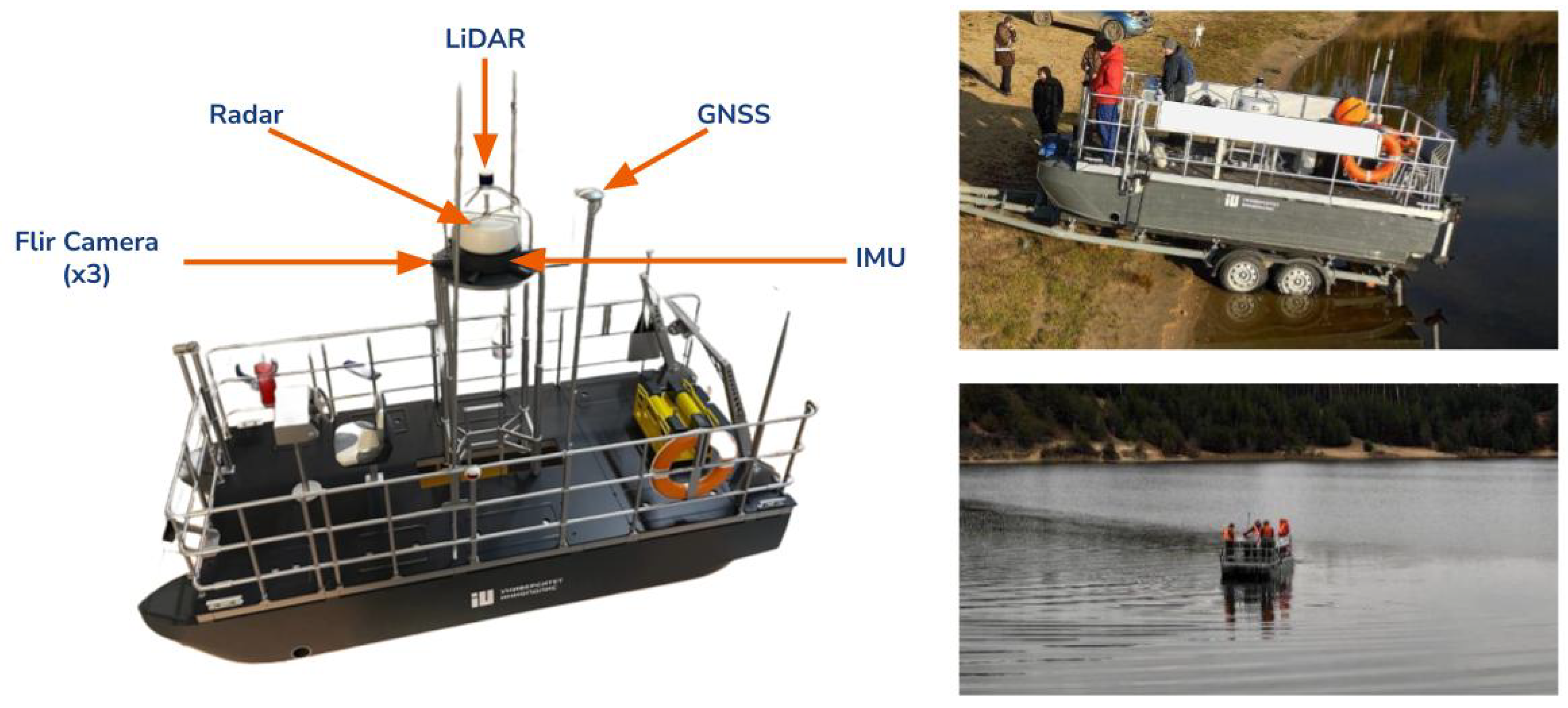
Our dataset consists of 428 GB of data collected through LiDAR, three RGB FLIR cameras, IMU, sonar, and GPS. These data were gathered during 2022–2023, and the dataset includes a wide range of objects such as ships, boats, buoys, pillars, and floating docks. The USV used for data collection is depicted in Figure 6. It is equipped with an advanced sensor suite to facilitate accurate and reliable dynamic object detection in challenging maritime environments.

The USV configuration includes the following key components:

• LiDAR for generating point cloud data that help to detect objects and determine their spatial positions in real time.
• IMU to correct for boat tilt, which can introduce distortions in the sensor data.
• GNSS for accurate location tracking, ensuring that objects are correctly localized even when the USV is in motion.
• Radar to improve detection capability under poor visibility conditions, such as fog or nighttime.
• FLIR cameras to capture visual data that complement the LiDAR and radar readings, especially for temperature-sensitive detections.

This comprehensive sensor suite allowed for the fusion of multiple data inputs, ensuring accurate detection and localization of objects in a wide range of maritime conditions. The USV was deployed in various real-world scenarios, providing critical data for evaluating and refining our proposed pipeline.

4.1.2. Simulation Data

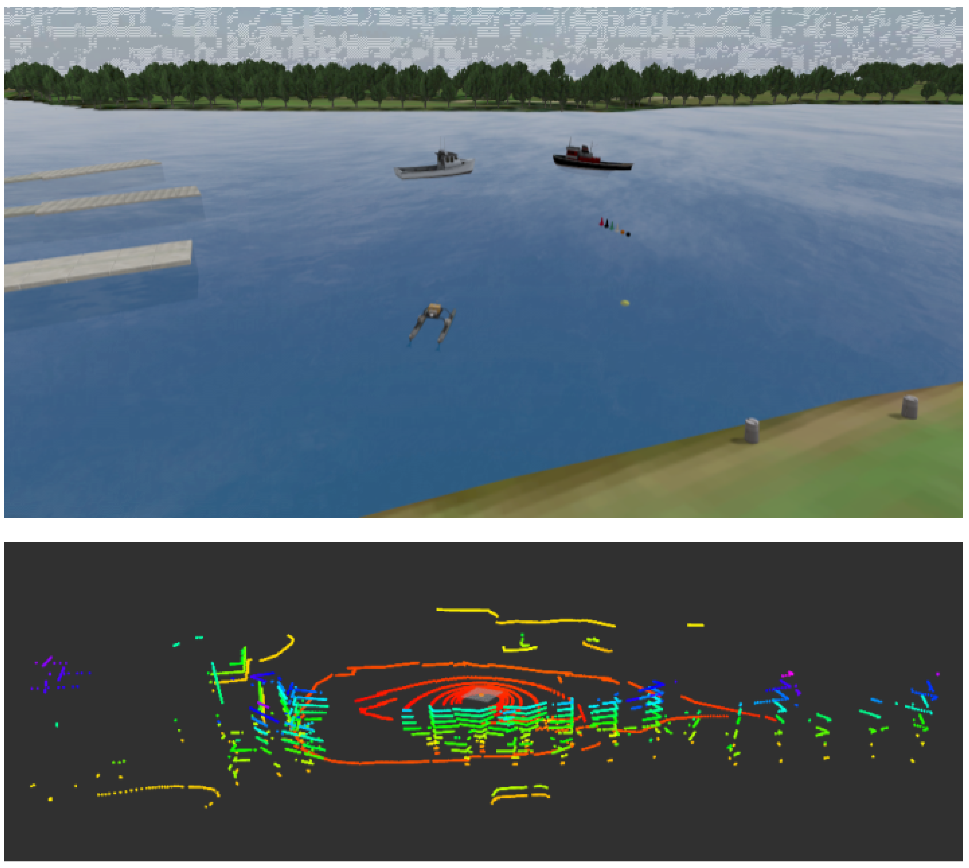
We used the VRX environment to evaluate our approaches in controlled environment dynamics where the ground truth of dynamic objects can be obtained, as shown in Figure 7. The VRX environment is built on Gazebo Garden and ROS2 for simulating maritime different scenarios. This setup contains a boat equipped with a LiDAR, GPS, IMU, and camera. The VRX simulator includes wave effects to simulate dynamic water conditions, along with various objects that can be added to the environment for evaluation purposes. This simulation enabled precise ground truth comparisons of object positioning and orientation, which was important for evaluating the efficiency of our pipeline.

4.2. Calibration

In our methodology, performing calibration between LiDAR and IMU sensors to obtain the offsets is crucial. This calibration enables us to correct the point cloud data influenced by the boat’s motion by fitting a plane to the water surface ripples and adjusting for roll, pitch, and yaw offsets, thereby ensuring that the LiDAR and IMU data accurately represent objects’ positions in the world frame.

4.3. Metrics

We employed two primary metrics for assessing our method’s effectiveness: the Root Mean Square Error (RMSE) for object position accuracy, and the detection rate for tracking performance.

4.3.1. Evaluating Preprocessing

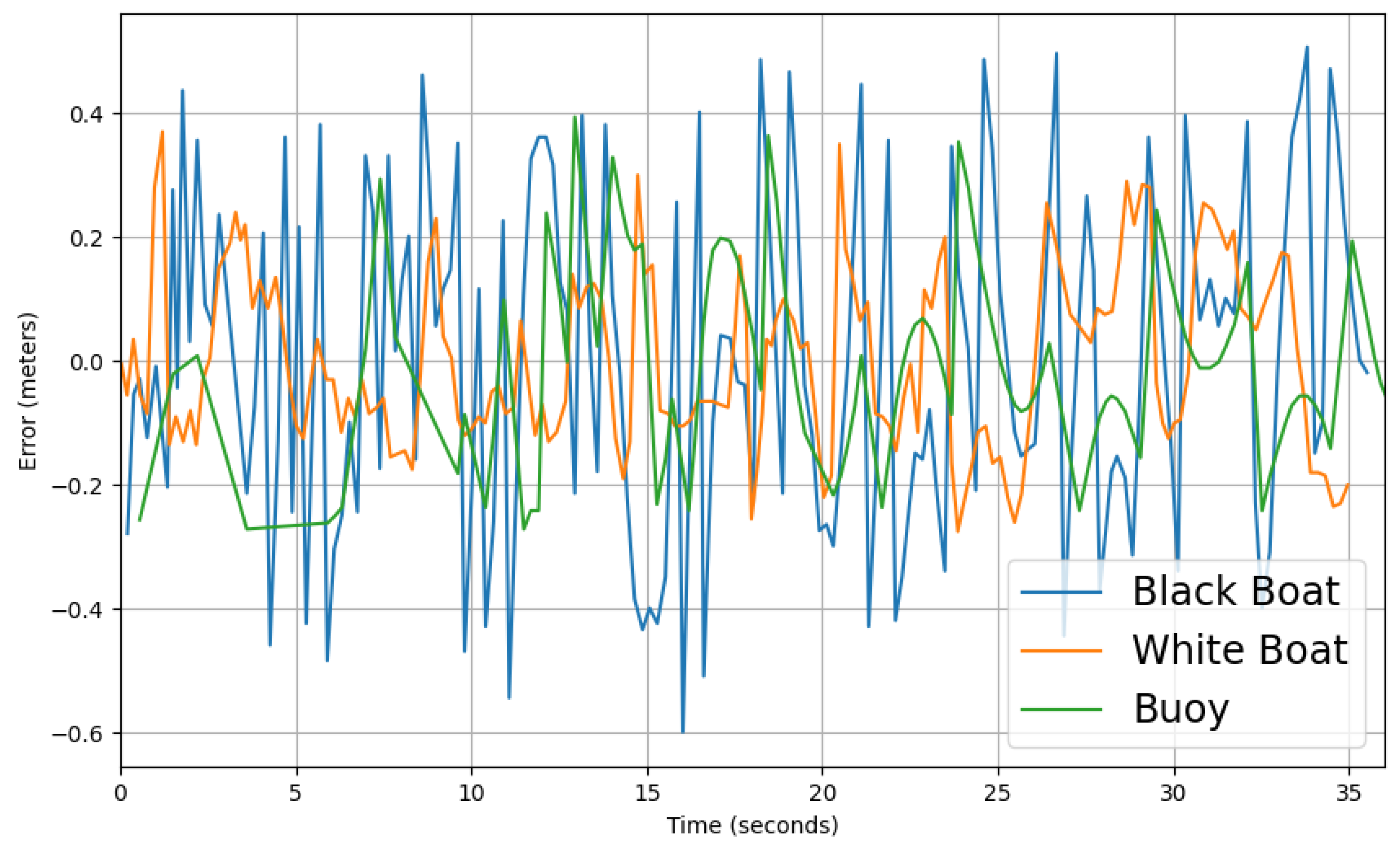
To evaluate the preprocessing part (point cloud stabilization), we use an error graph to measure the position error of each object with respect to the ground truth of the same object. In addition, the Root Mean Square Error (RMSE) is calculated and added to the table for comparison. During the evaluation, the investigation for each object was carried out for 35 s in a controlled environment. Figure 8 and Figure 9 show the impact of the preprocessing step in correcting the position of each object to ensure that it represents the correct position in the real world. In this test, we used three objects: a white boat, a black boat, and a buoy. Their known ground truth positions are listed in

Table 1. Objects’ ground truth coordinates.

Objects	[X, Y, Z] Coordinates (m)
Black Boat	[74.50, −16.00, 1.50]
White Boat	[29.40, 24.80, 1.40]
Buoy	[27.60, 10.00, 0.51]

, with the coordinates provided in the form $[X,Y,Z]$, where X, Y, and Z represent the positions along the respective axes in the real-world environment.

The results are presented in Figure 8 and Figure 9. The Root Mean Square Error (RMSE) was calculated and is included in

Table 2. Root mean square error (meters).

	Black Boat	White Boat	Buoy
Before preprocessing	2.316	0.549	0.636
After preprocessing	0.269	0.141	0.157
Preprocessing + Kalman Filter	0.070	0.037	0.041

. The table shows the RMSE of the detected objects in meters at different stages of the pipeline:

• Before Preprocessing: RMSE values when raw sensor data are used without any processing.
• After Preprocessing: RMSE values after stabilizing the LiDAR data and removing noise.
• After Preprocessing with Kalman Filtering (KF): RMSE values after preprocessing and applying the Kalman filter for smoothing and improving the accuracy of object tracking. The Kalman filter is a mathematical algorithm used to estimate the state of an object in motion, thereby reducing errors and noise.

Abbreviations: KF stands for Kalman Filter.

In Figure 8, a sine wave can be seen; this is because of the nature of waves in water, which form a sine wave. There are several other points worth mentioning as well. First, the peaks are not equal, which is due to the waves not having the same strength over time. Second, the amplitude of the upper peaks is sometime higher that of the lower peaks, and vice versa; this is caused by interference between two sine waves (one wave that moves our boat up and down and another that moves the target up and down),resulting in the upper and lower peaks having different amplitudes, Lastly, and most importantly, it can be seen that the sine wave amplitude (peak) is greater for some objects than for others; this is due to the fact that the boat tilt causes more distant objects to have a larger error with respect to the ground truth, as a small tilt in the roll or pitch angle of our boat translates to a large variation in the vertical distance of the target object.

In Figure 9, it can be seen that the error falls from 2.31 (m) to 26.9 (cm) after preprocessing, representing a huge decrease and showing the good effect of the preprocessing stage in stabilizing the surrounding objects. However, part of the error is due to the fact that the rays that hit the target object position change when our boat tilts. We can imagine a case in which a boat is being hit by two laser rings on the upper part, then our boat tilts; thus, the same object is still being hit by two laser rings, except now on the lower part, causing the object’s center coordinates to be changed due to the change in where it is being hit by the laser beams. In order to eliminate this part of the error, we use the Kalman filter-based tracker.

Table 1 shows the relative positions of the three experimental objects to our boat in meters (x, y, z).

Table 2 shows the RMSE values of the positions of the three experimental objects with respect to their ground truth positions.

4.3.2. Evaluating the Tracker (Kalman Filter)

To evaluate the tracker, we use the square error for the graph to show the correctness of object tracking and the mean square error to assess the further improvement added in the preprocessing step to overcome bounding box movement due to rays hitting different parts of the boat. We also use the detection rate, as the Kalman filter has a prediction step, meaning that it should overperform compared to detection-only techniques thanks to its ability to predict the position of the object even in frames where the points of an object are lost. For the detection rate, we want to determine how many times the objects are detected correctly through multiple consecutive frames, where “detected correctly” means that the IoU of the tracked bounding box should be at least 0.5 compared to the ground truth bounding box; this number is divided by the total number of frames, meaning that if we have 100 frames and 90 of them are being tracked correctly in the correct position, then the detection rate will be 90%.

To achieve this, we track the same three objects for 35 s and show the impact of tracking on correcting and predicting the accurate position of objects.

Figure 10 and Table 2 show that the Kalman filter reduces the error of the black boat from 26.9 cm to 7 cm, the error of the white boat from 14.1 cm to 3.7 cm, and the error of the buoy from 15.7 cm to 4.1 cm.

Table 3. Detection rate (%).

	Black Boat	White Boat	Buoy
before preprocessing	4.7	5.6	4.3
after preprocessing	50.5	55.6	45.4
preprocessing + KF	78.3	82.4	77.5

shows that the rate of detection for the three objects before preprocessing is almost 5%; all three objects are represented in the wrong places due to the fluctuating motion of our USV. After preprocessing, a huge performance boost can be seen after correcting the position of those objects; however, we are still not close to 100% due to the LiDAR not being able to detect an object in all frames. Although the field of view (FOV) of the LiDAR sometimes does not include the object, adding the tracker has a positive effect on detection, providing more accurate position output and preventing sudden jumps. In addition, the tracking stage includes a prediction step, which allowing the object to be predicted in future frames even if it is not detected in the current frame. This prediction is made based on the speed and orientation of the object, increasing the detection rate by 25% to 30%.

4.4. Results and Discussion

Our experiments demonstrate significant improvements in detecting and tracking dynamic objects, particularly in environments with motion-induced fluctuations. The preprocessing steps, including point cloud stabilization, play a crucial role in reducing errors caused by sensor movement and environmental interference. This improvement is reflected in the reduced Root Mean Square Error (RMSE) for object positions, especially after applying the Kalman filter. The RMSE values for the black boat, white boat, and buoy showed notable reductions after preprocessing, and further improvements were observed after integrating the Kalman filter. The RMSE values before preprocessing were 2.316 m, 0.549 m, and 0.636 m for the black boat, white boat, and buoy, respectively. After preprocessing, these values dropped significantly to 0.269 m, 0.141 m, and 0.157 m. The application of the Kalman filter further reduced these errors to 0.070 m, 0.037 m, and 0.041 m, demonstrating the effectiveness of our method in stabilizing object positions and improving tracking accuracy.

Additionally, the detection rate metric provided insights into the performance of the tracking system. Before preprocessing, the detection rates for the black boat, white boat, and buoy were 4.7%, 5.6%, and 4.3%, respectively; after preprocessing, these rates improved to 50.5%, 55.6%, and 45.4%. The integration of the Kalman filter boosted the detection rates to 78.3%, 82.4%, and 77.5%. This increase is attributed to the Kalman filter’s ability to predict object positions even when LiDAR points are not detected in certain frames, enhancing both the accuracy and consistency of the tracking system.

The combination of preprocessing and Kalman filter-based tracking proves highly effective in marine dynamic object detection and tracking. The substantial reduction in RMSE and the marked improvement in the detection rate across all tested objects confirm the robustness and reliability of the proposed method. These results underline the potential of our approach for real-time applications in challenging marine environments, where precise object tracking is essential despite the presence of environmental factors such as water waves and sensor motion. The proposed methodology successfully addresses these challenges, ensuring more accurate and stable identification of moving objects in marine settings.

5. Conclusions

In this paper, we have presented a comprehensive approach to object detection and tracking for USVs in maritime environments by integrating IMU and LiDAR sensor data. Our approach introduces a novel data fusion technique that effectively corrects for tilt-induced distortions in the LiDAR point clouds, ensuring accurate object positioning and significantly reducing the complexities introduced by water ripples and boat movements. We realize improve object delineation and encapsulation within bounding boxes by enhancing the quality of the data fed into our clustering algorithm. However, there is some discontinuity in object tracking because of the sparsity of the data and the occasional loss of objects across frames. To address this problem, we develop and implement a robust Kalman Filter, introducing improvements intended specifically for maritime sensors. As a result, it is possible to maintain continuity even in instances where objects are sparsely represented or momentarily obscured. We evaluated our approach using the metrics of RMSE for preprocessing accuracy and detection rate for the tracking stage. This evaluation underscored the effectiveness of our approach, with the results exhibiting a significant improvement in the precision of object location across consecutive frames. The evaluation results affirm the robustness of our method in the face of challenges such as object sparsity and intermittent visibility. Afterwards, we moved to validation. We first validated our approach through simulation in order to fine-tune our system. Then, we conducted real-world experiments in the Volga River with an actual USV. These experiments provided practical evidence of the applicability and efficiency of our approach in real maritime settings and confirmed its operational viability. To sum up, our proposed pipeline proved reliable and accurate and performed well in dynamic maritime conditions. In the future, safer and more autonomous maritime navigation can be achieved by integrating more sensors and applying new machine learning techniques to further enhance the detection and tracking capabilities of our proposed approach.

References

1. Yan, R.-J.; Pang, S.; Sun, H.-B.; Pang, Y.-J. Development and missions of unmanned surface vehicle. J. Mar. Sci. Appl. 2010, 9, 451–457. [Google Scholar] [CrossRef]
2. Barrera, C.; Padron, I.; Luis, F.S.; Llinas, O. Trends and challenges in unmanned surface vehicles (USV): From survey to shipping. Trans. Nav. Int. J. Mar. Navig. Saf. Sea Transp. 2021, 15, 135–142. [Google Scholar] [CrossRef]
3. Li, J.; Zhang, G.; Jiang, C.; Zhang, W. A survey of maritime unmanned search system: Theory, applications and future directions. Ocean Eng. 2023, 285, 115359. [Google Scholar] [CrossRef]
4. Bae, I.; Hong, J. Survey on the developments of unmanned marine vehicles: Intelligence and cooperation. Sensors 2023, 23, 4643. [Google Scholar] [CrossRef]
5. Bai, X.; Li, B.; Xu, X.; Xiao, Y. A review of current research and advances in unmanned surface vehicles. J. Mar. Sci. Appl. 2022, 21, 47–58. [Google Scholar] [CrossRef]
6. Patterson, R.G.; Lawson, E.; Udyawer, V.; Brassington, G.B.; Groom, R.A.; Campbell, H.A. Uncrewed surface vessel technological diffusion depends on cross-sectoral investment in open-ocean archetypes: A systematic review of USV applications and drivers. Front. Mar. Sci. 2022, 8, 736984. [Google Scholar] [CrossRef]
7. Jain, S.; Nuske, S.; Chambers, A.; Yoder, L.; Cover, H.; Chamberlain, L.; Scherer, S.; Singh, S. Autonomous River Exploration. In Field and Service Robotics; Springer: Cham, Switzerland, 2015; pp. 93–106. [Google Scholar]
8. Scherer, S.; Rehder, J.; Achar, S.; Cover, H.; Chambers, A.; Nuske, S.; Singh, S. River mapping from a flying robot: State estimation, river detection, and obstacle mapping. Auton. Robot. 2012, 33, 189–214. [Google Scholar] [CrossRef]
9. Zhan, W.; Xiao, C.; Wen, Y.; Zhou, C.; Yuan, H.; Xiu, S.; Zhang, Y.; Zou, X.; Liu, X.; Li, Q. Autonomous visual perception for unmanned surface vehicle navigation in an unknown environment. Sensors 2019, 19, 2216. [Google Scholar] [CrossRef]
10. Huntsberger, T.; Aghazarian, H.; Howard, A.; Trotz, D. Stereo vision–based navigation for autonomous surface vessels. J. Field Robot. 2011, 28, 3–18. [Google Scholar] [CrossRef]
11. Martins, A.; Almeida, J.; Ferreira, H.; Silva, H.; Dias, N.; Dias, A.; Almeida, C.; Silva, E. Autonomous Surface Vehicle Docking Manoeuvre with Visual Information. In Proceedings of the 2007 IEEE International Conference on Robotics And Automation, Rome, Italy, 10–14 April 2007; pp. 4994–4999. [Google Scholar]
12. Chang, S.; Deng, Y.; Zhang, Y.; Zhao, Q.; Wang, R.; Zhang, K. An advanced scheme for range ambiguity suppression of spaceborne SAR based on blind source separation. IEEE Trans. Geosci. Remote Sens. 2022, 60, 5230112. [Google Scholar] [CrossRef]
13. Han, J.; Park, J.; Kim, T.; Kim, J. Precision navigation and mapping under bridges with an unmanned surface vehicle. Auton. Robot. 2015, 38, 349–362. [Google Scholar] [CrossRef]
14. Crasto, N.; Hopkinson, C.; Forbes, D.; Lesack, L.; Marsh, P.; Spooner, I.; Van Der Sanden, J. A LiDAR-based decision-tree classification of open water surfaces in an Arctic delta. Remote Sens. Environ. 2015, 164, 90–102. [Google Scholar] [CrossRef]
15. Li, Y.; Ma, L.; Zhong, Z.; Liu, F.; Chapman, M.A.; Cao, D.; Li, J. Deep Learning for LiDAR Point Clouds in Autonomous Driving: A Review. IEEE Trans. Neural Netw. Learn. Syst. 2021, 32, 3412–3432. [Google Scholar] [CrossRef]
16. Jeong, M.; Li, A.Q. Efficient Lidar-based in-Water Obstacle Detection and Segmentation by Autonomous Surface Vehicles in Aquatic Environments. In Proceedings of the 2021 IEEE/RSJ International Conference on Intelligent Robots and Systems (IROS), Prague, Czech Republic, 27 September–1 October 2021; IEEE: New York, NY, USA, 2021; pp. 5387–5394. [Google Scholar]
17. Kumar, G.S.; Painumgal, U.V.; Kumar, M.C.; Rajesh, K.H. Autonomous underwater vehicle for vision based tracking. Proc. Comput. Sci. 2018, 133, 169–180. [Google Scholar] [CrossRef]
18. Wang, L.; Xiao, Y.; Zhang, B.; Liu, R.; Zhao, B. Water Surface Targets Detection Based on the Fusion of Vision and LiDAR. Sensors 2023, 23, 1768. [Google Scholar] [CrossRef] [PubMed] [PubMed Central]
19. Thompson, D. Maritime Object Detection, Tracking, and Classification Using LiDAR and Vision-Based Sensor Fusion. Master’s Thesis, Embry-Riddle Aeronautical University, Daytona Beach, FL, USA, 2017. [Google Scholar]
20. Hsu, C.-W.; Lin, C.-J. A comparison of methods for multiclass support vector machines. IEEE Trans. Neural Netw. 2002, 13, 415–425. [Google Scholar]
21. Yao, X.; Shan, Y.; Li, J.; Ma, D.; Huang, K. LiDAR based Navigable Region Detection for Unmanned Surface Vehicles. In Proceedings of the 2019 IEEE/RSJ International Conference on Intelligent Robots And Systems (IROS), Macau, China, 3–8 November 2019; pp. 3754–3759. [Google Scholar]
22. Shan, Y.; Yao, X.; Lin, H.; Zou, X.; Huang, K. LiDAR-Based Stable Navigable Region Detection for Unmanned Surface Vehicles. IEEE Trans. Instrum. Meas. 2021, 70, 8501613. [Google Scholar] [CrossRef]
23. Edwan, E.; Knedlik, S.; Loffeld, O. Constrained angular motion estimation in a gyro-free IMU. IEEE Trans. Aerosp. Electron. Syst. 2011, 47, 596–610. [Google Scholar] [CrossRef]
24. Cardou, P.; Angeles, J. Estimating the angular velocity of a rigid body moving in the plane from tangential and centripetal acceleration measurements. Multibody Syst. Dyn. 2008, 19, 383–406. [Google Scholar] [CrossRef]
25. Morin, D. Introduction to Classical Mechanics: With Problems and Solutions; Cambridge University Press: Cambridge, UK, 2008. [Google Scholar]
26. Kleppner, D.; Kolenkow, R. An Introduction to Mechanics; Cambridge University Press: Cambridge, UK, 2014. [Google Scholar]
27. Sun, Z.; Li, Z.; Liu, Y. An Improved Lidar Data Segmentation Algorithm based on Euclidean Clustering. In Proceedings of the 11th International Conference on Modelling, Identification and Control (ICMIC2019), Tianjin, China, 13–15 July 2019; pp. 1119–1130. [Google Scholar]
28. Ahmed, S.M.; Chew, C.M. Density-based Clustering for 3D Object Detection in Point Clouds. In Proceedings of the IEEE/CVF Conference on Computer Vision and Pattern Recognition, Seattle, WA, USA, 13–19 June 2020; pp. 10608–10617. [Google Scholar]
29. Vo, A.; Truong-Hong, L.; Laefer, D.; Bertolotto, M. Octree-based region growing for pointcloud segmentation. ISPRS J. Photogramm. Remote Sens. 2015, 104, 88–100. [Google Scholar] [CrossRef]
30. Ankerst, M.; Breunig, M.; Kriegel, H.-P.; Ng, R.; Sander, J. OPTICS: Ordering Points to Identify the Clustering Structure. In Proceedings of the ACM SIGMOD International Conference on Management of Data (SIGMOD’99), Philadelphia, PA, USA, 1–3 June 1999; ACM: New York, NY, USA, 2008. [Google Scholar]
31. Dockhorn, A.; Braune, C.; Kruse, R. An Alternating Optimization Approach based on Hierarchical Adaptations of DBSCAN. In Proceedings of the 2015 IEEE Symposium Series on Computational Intelligence, Cape Town, South Africa, 7–10 December 2015; IEEE: New York, NY, USA, 2015; pp. 749–755. [Google Scholar]
32. Sahu, N.K. DBSCAN & hierarchical clustering algorithm: Analysis cyber crime data. Int. J. Multidiscip. Educ. Res. 2022, 11, 16–20. [Google Scholar]
33. Latifi-Pakdehi, A.; Daneshpour, N. DBHC: A DBSCAN-based hierarchical clustering algorithm. Data Knowl. Eng. 2021, 135, 101922. [Google Scholar] [CrossRef]
34. Abdi, H.; Williams, L.J. Principal component analysis. Wiley Interdiscip. Rev. Comput. Stat. 2010, 2, 433–459. [Google Scholar] [CrossRef]
35. Shlens, J. A tutorial on principal component analysis. arXiv 2014, arXiv:1404.1100. [Google Scholar]
36. Wold, S.; Esbensen, K.; Geladi, P. Principal component analysis. Chemom. Intell. Lab. Syst. 1987, 2, 37–52. [Google Scholar] [CrossRef]
37. Maćkiewicz, A.; Ratajczak, W. Principal components analysis (PCA). Comput. Geosci. 1993, 19, 303–342. [Google Scholar] [CrossRef]
38. Kuhn, H.W. The Hungarian method for the assignment problem. Nav. Res. Logist. Q. 1955, 2, 83–97. [Google Scholar] [CrossRef]
39. Fielding, G.; Kam, M. Applying the Hungarian Method to Stereo Matching. In Proceedings of the 36th IEEE Conference on Decision and Control, San Diego, CA, USA, 12 December 1997; IEEE: New York, NY, USA, 1997; Volume 2, pp. 1928–1933. [Google Scholar]
40. Hamuda, E.; Mc Ginley, B.; Glavin, M.; Jones, E. Improved image processing-based crop detection using Kalman filtering and the Hungarian algorithm. Comput. Electron. Agric. 2018, 148, 37–44. [Google Scholar] [CrossRef]
41. Chen, S.-Y. Kalman filter for robot vision: A survey. IEEE Trans. Ind. Electron. 2011, 59, 4409–4420. [Google Scholar] [CrossRef]
42. Chan, Y.T.; Hu, A.G.C.; Plant, J.B. A Kalman filter based tracking scheme with input estimation. IEEE Trans. Aerosp. Electron. Syst. -15.
43. Wang, Z.; Walsh, K.; Koirala, A. Mango fruit load estimation using a video based MangoYOLO—Kalman filter—Hungarian algorithm method. Sensors 2019, 19, 2742. [Google Scholar] [CrossRef]
44. Jonker, R.; Volgenant, T. A Shortest Augmenting Path Algorithm for Dense and Sparse Linear Assignment Problems. In DGOR/NSOR: Papers of the 16th Annual Meeting of DGOR in Cooperation with NSOR/Vorträge der 16. Jahrestagung der DGOR Zusammen mit der NSOR; Springer: Berlin/Heidelberg, Germany, 1988; p. 622. [Google Scholar]
45. Bertsekas, D.P. Auction algorithms for network flow problems: A tutorial introduction. Comput. Optim. Appl. 1992, 1, 7–66. [Google Scholar] [CrossRef]
46. Welch, G.; Bishop, G. An Introduction to the Kalman Filter; University of North Carolina: Chapel Hill, NC, USA, 1995. [Google Scholar]
47. Wiseman, Y. Ancillary ultrasonic rangefinder for autonomous vehicles. Int. J. Secur. Its Appl. 2018, 12, 49–58. [Google Scholar] [CrossRef]
48. Premnath, S.; Mukund, S.; Sivasankaran, K.; Sidaarth, R.; Adarsh, S. Design of an Autonomous Mobile Robot based on the Sensor Data Fusion of LIDAR 360, Ultrasonic Sensor and Wheel Speed Encoder. In Proceedings of the 2019 9th International Conference on Advances in Computing and Communication (ICACC), Kochi, India, 6–8 November 2019; IEEE: New York, NY, USA, 2019; pp. 62–65. [Google Scholar]
49. Bingham, B.; Aguero, C.; McCarrin, M.; Klamo, J.; Malia, J.; Allen, K.; Lum, T.; Rawson, M.; Waqar, R. Toward Maritime Robotic Simulation in Gazebo. In Proceedings of the MTS/IEEE OCEANS Conference, Seattle, WA, USA, 27–31 October 2019. [Google Scholar]
Figure 1. Abstract overview of the Seal Pipeline.
Drones 08 00561 g001
Figure 2. Sensor−derived Data: (a) LiDAR-captured point cloud depicting a large vessel and the noise generated by our boat’s trailing wake; (b) RS-LiDAR-32 laser distribution pattern.
Drones 08 00561 g002
Figure 3. Clustered objects in the boat’s environment.
Drones 08 00561 g003
Figure 4. The boat’s forward orientation corresponds to the point cloud’s backward orientation in the LiDAR frame coordinate system.
Drones 08 00561 g004
Figure 5. Point cloud representation before and after preprocessing: (a) before preprocessing, showing distortions and noise; (b) after preprocessing, showing refined high-quality data.
Drones 08 00561 g005
Figure 6. The USV used for conducting experiments in the Volga River. This USV is equipped with LiDAR, three FLIR cameras, radar, IMU, GNSS, and sonar for comprehensive data collection and sensor fusion.
Drones 08 00561 g006
Figure 7. The VRX environment with Gazebo simulator [49], represented in the upper figure, and rviz2 visualizer for showing the point cloud data from the boat, represented in the lower figure.
Drones 08 00561 g007
Figure 8. Position error of different objects after the preprocessing step (stabilization); the error is calculated using the ground truth position of the object as the reference.
Drones 08 00561 g008
Figure 9. Preprocessing step (stabilization); the error is calculated using the ground truth position of the object as the reference.
Drones 08 00561 g009
Figure 10. Position errors of different objects after the preprocessing step (stabilization) and Kalman filter tracking; the error is calculated using the ground truth position of the object as the reference.
Drones 08 00561 g010