
Multi-UAV Path Planning and Following Based on Multi-Agent Reinforcement Learning


Abstract
1. Introduction
- Establishing a multi-UAV simulation environment to train and validate the proposed approach. It involves individual interactions between agents and the environment, avoiding joint action and state spaces. This prevents exponential parameter growth with an increasing number of agents and maintains linearity.
- Proposing a parameter-sharing off-policy multi-agent path planning and following an approach that leverages interaction data from all agents. Experimental simulation results validate its effectiveness.
- Designing a reward function that encourages UAV movement, addressing the problem of UAVs remaining stationary in the initial phase and exhibiting overly cautious and minimal actions when approaching the goal.
2. Approach
2.1. Soft Actor–Critic
| Algorithm 1 Soft actor–critic |
|
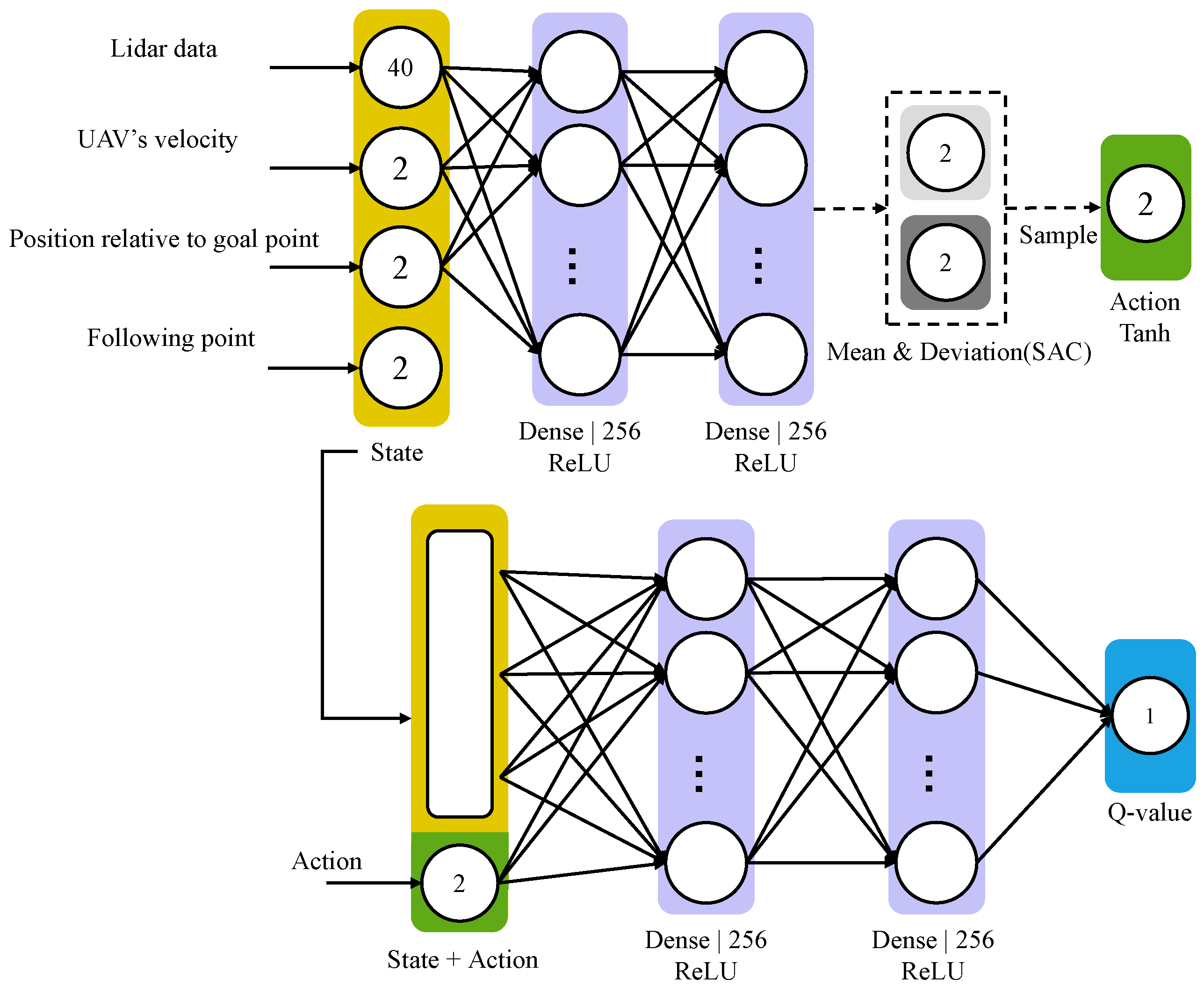
2.2. Network Structure
2.3. Multi-Agent Framework
2.4. Reward Function Design
3. Experiment and Result
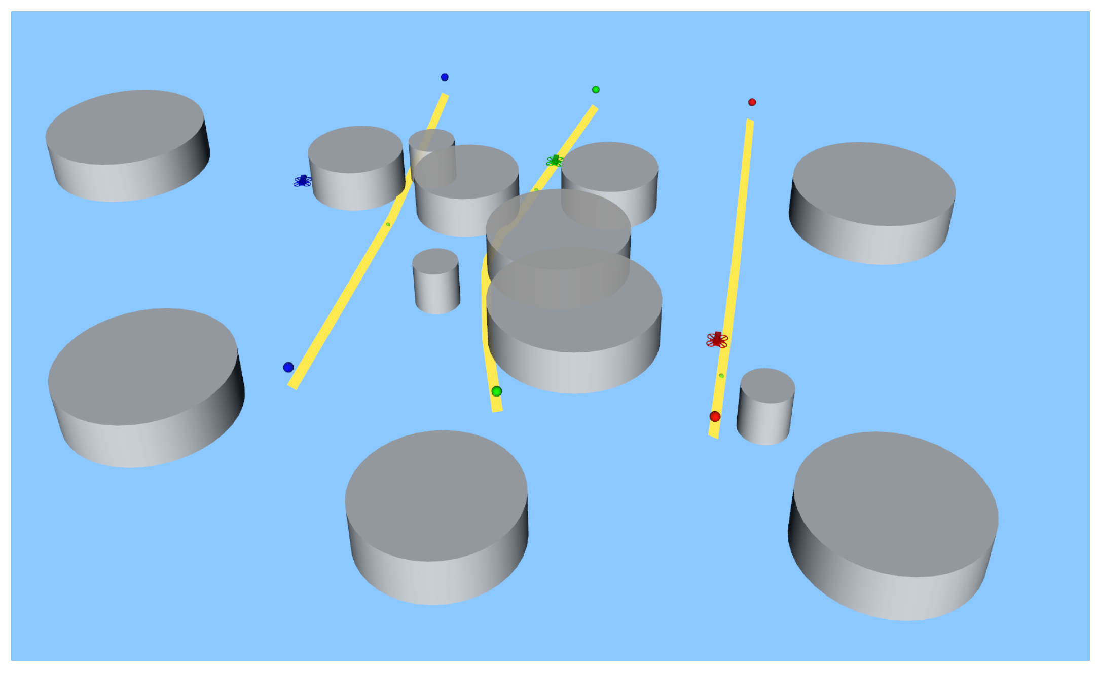
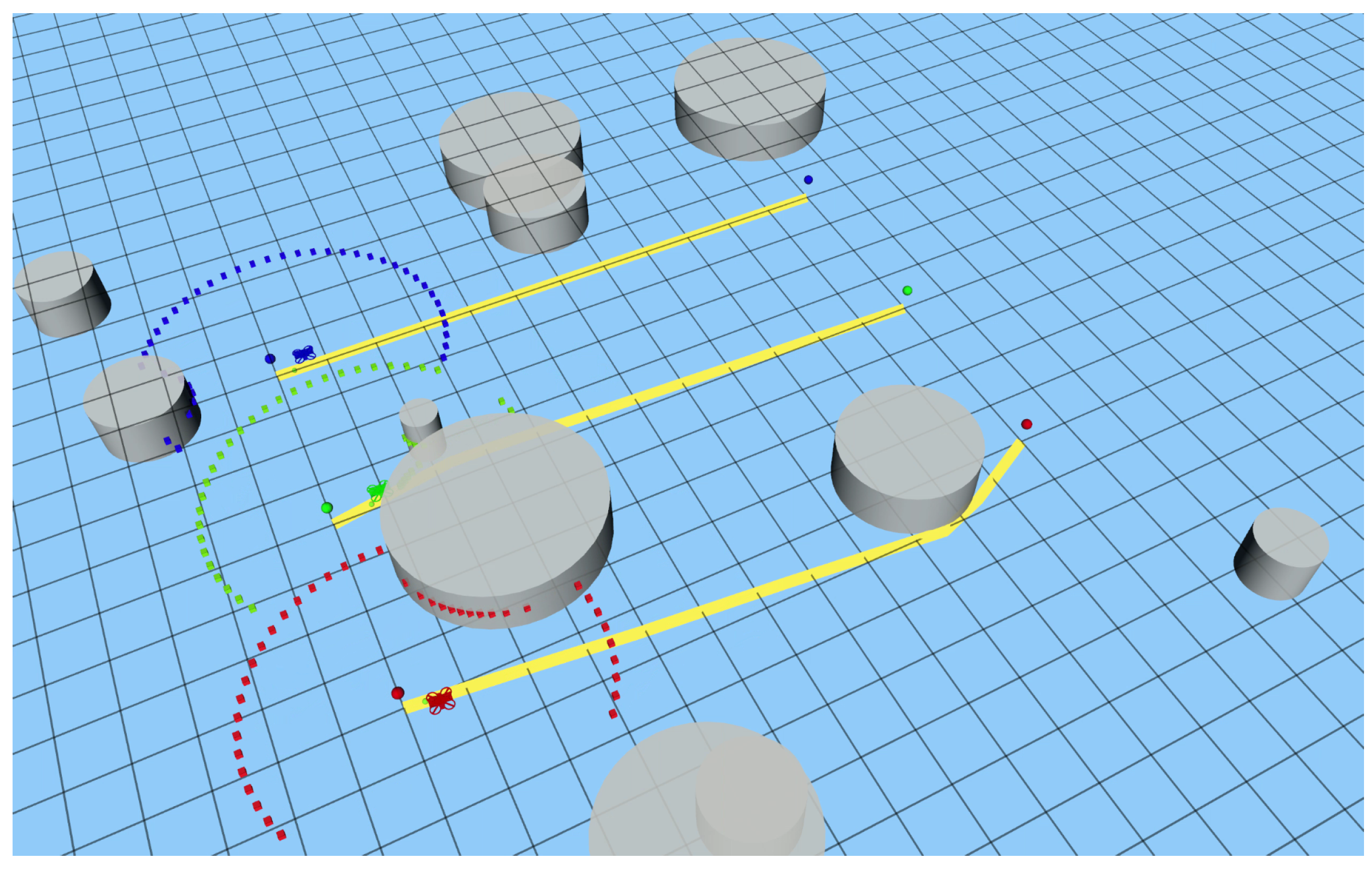
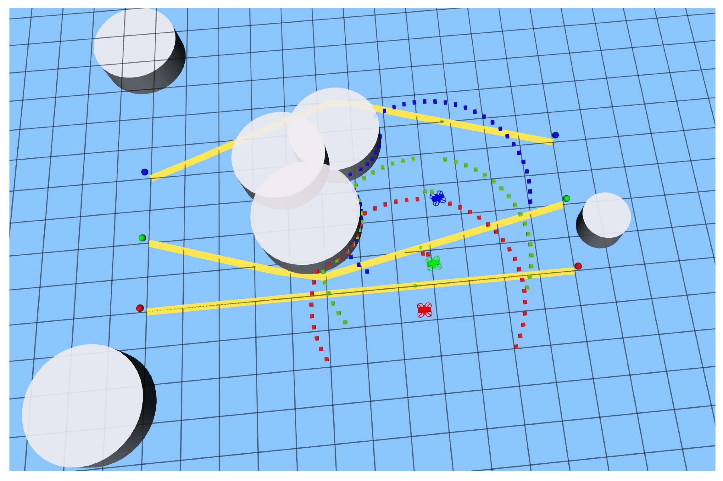
3.1. Simulation Environment
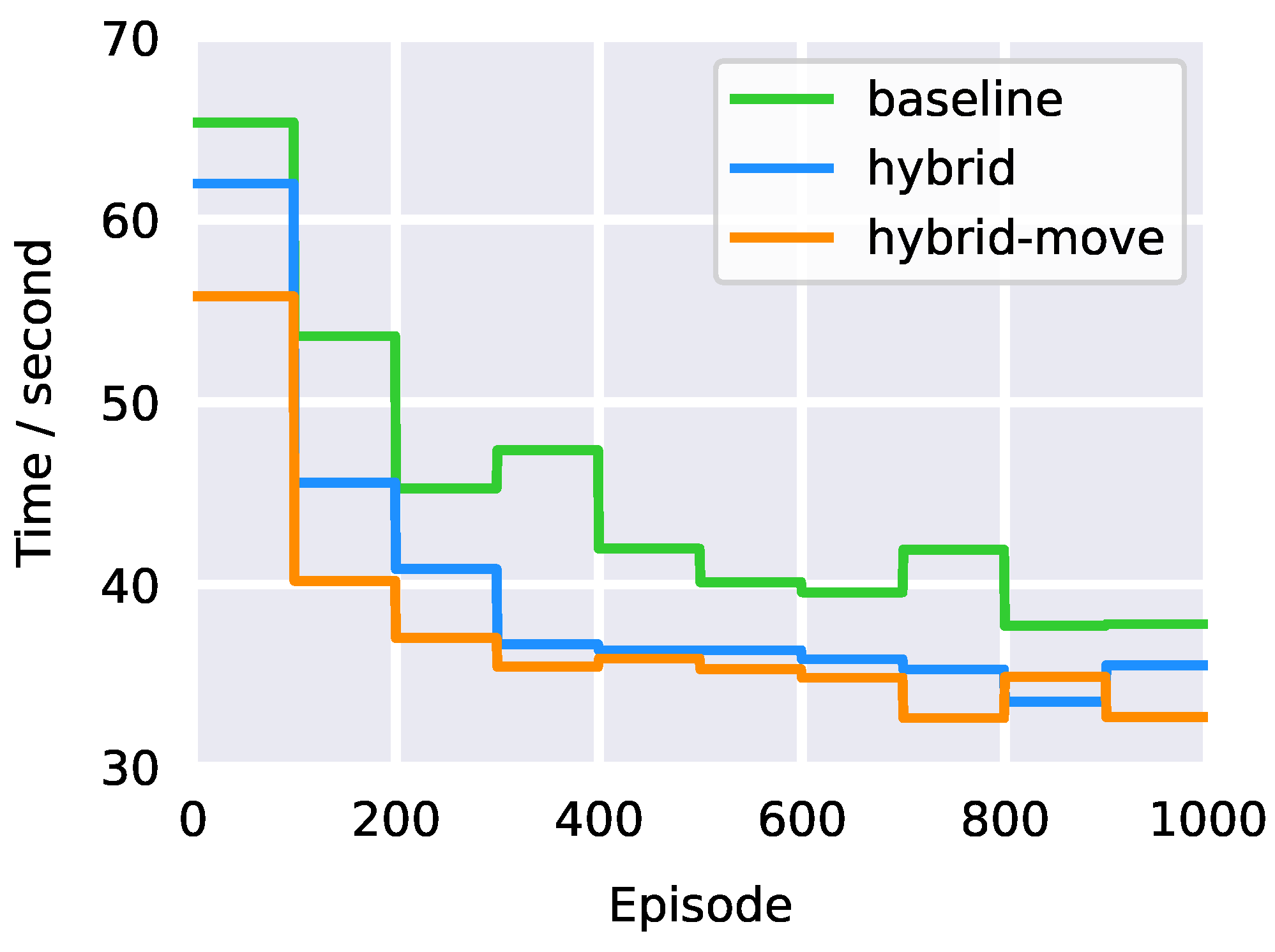
3.2. Results and Discussion
4. Conclusions
Author Contributions
Funding
Institutional Review Board Statement
Informed Consent Statement
Data Availability Statement
Conflicts of Interest
Abbreviations
| SAC | Soft actor–critic |
| RRT | Rapidly exploring random tree |
| DRL | Deep reinforcement learning |
| AIT* | Adaptively informed trees |
| SEAC | Shared experience actor–critic |
| MDP | Markov decision process |
| DDPG | Deep deterministic policy gradients |
| TD3 | Twin-delayed deep deterministic |
| KL | Kullback–Leibler |
| FC | Fully connected |
| IQL | Independent Q-learning |
| TD | Temporal difference |
| ROS | Robot operating system |
References
- Madridano, Á.; Al-Kaff, A.; Gómez, D.M.; de la Escalera, A. Multi-Path Planning Method for UAVs Swarm Purposes. In Proceedings of the 2019 IEEE International Conference on Vehicular Electronics and Safety (ICVES), Cairo, Egypt, 4–6 September 2019; pp. 1–6. [Google Scholar] [CrossRef]
- Lin, S.; Liu, A.; Wang, J.; Kong, X. A Review of Path-Planning Approaches for Multiple Mobile Robots. Machines 2022, 10, 773. [Google Scholar] [CrossRef]
- Fan, T.; Long, P.; Liu, W.; Pan, J. Distributed multi-robot collision avoidance via deep reinforcement learning for navigation in complex scenarios. Int. J. Robot. Res. 2020, 39, 856–892. [Google Scholar] [CrossRef]
- Ait Saadi, A.; Soukane, A.; Meraihi, Y.; Benmessaoud Gabis, A.; Mirjalili, S.; Ramdane-Cherif, A. UAV Path Planning Using Optimization Approaches: A Survey. Arch. Comput. Methods Eng. 2022, 29, 4233–4284. [Google Scholar] [CrossRef]
- Mechali, O.; Xu, L.; Wei, M.; Benkhaddra, I.; Guo, F.; Senouci, A. A Rectified RRT* with Efficient Obstacles Avoidance Method for UAV in 3D Environment. In Proceedings of the 2019 IEEE 9th Annual International Conference on CYBER Technology in Automation, Control, and Intelligent Systems (CYBER), Suzhou, China, 29 July–2 August 2019; pp. 480–485. [Google Scholar] [CrossRef]
- Chen, T.; Zhang, G.; Hu, X.; Xiao, J. Unmanned Aerial Vehicle Route Planning Method Based on a Star Algorithm. In Proceedings of the 2018 13th IEEE Conference on Industrial Electronics and Applications (ICIEA), Wuhan, China, 31 May–2 June 2018; pp. 1510–1514. [Google Scholar] [CrossRef]
- Wu, J.; Shin, S.; Kim, C.G.; Kim, S.D. Effective Lazy Training Method for Deep Q-Network in Obstacle Avoidance and Path Planning. In Proceedings of the 2017 IEEE International Conference on Systems, Man, and Cybernetics (SMC), Banff, AB, Canada, 5–8 October 2017; pp. 1799–1804. [Google Scholar] [CrossRef]
- Dewangan, R.K.; Shukla, A.; Godfrey, W.W. Survey on prioritized multi robot path planning. In Proceedings of the 2017 IEEE International Conference on Smart Technologies and Management for Computing, Communication, Controls, Energy and Materials (ICSTM), Chennai, India, 2–4 August 2017; pp. 423–428. [Google Scholar] [CrossRef]
- Stern, R. Multi-Agent Path Finding—An Overview. In Artificial Intelligence; Springer: Cham, Switzerland, 2019; pp. 96–115. [Google Scholar] [CrossRef]
- Canese, L.; Cardarilli, G.C.; Di Nunzio, L.; Fazzolari, R.; Giardino, D.; Re, M.; Spanò, S. Multi-Agent Reinforcement Learning: A Review of Challenges and Applications. Appl. Sci. 2021, 11, 4948. [Google Scholar] [CrossRef]
- Bennewitz, M.; Burgard, W.; Thrun, S. Optimizing schedules for prioritized path planning of multi-robot systems. In Proceedings of the Proceedings 2001 ICRA, IEEE International Conference on Robotics and Automation (Cat. No.01CH37164), Seoul, Republic of Korea, 21–26 May 2001; Volume 1, pp. 271–276. [Google Scholar] [CrossRef]
- Wang, W.; Goh, W.B. Time Optimized Multi-Agent Path Planning Using Guided Iterative Prioritized Planning. In Proceedings of the 2013 International Conference on Autonomous Agents and Multi-Agent Systems, AAMAS’13, Saint Paul, MN, USA, 6–10 May 2013; pp. 1183–1184. [Google Scholar]
- Desaraju, V.R.; How, J.P. Decentralized path planning for multi-agent teams in complex environments using rapidly exploring random trees. In Proceedings of the 2011 IEEE International Conference on Robotics and Automation, Shanghai, China, 9–13 May 2011; pp. 4956–4961. [Google Scholar] [CrossRef]
- Nazarahari, M.; Khanmirza, E.; Doostie, S. Multi-objective multi-robot path planning in continuous environment using an enhanced genetic algorithm. Expert Syst. Appl. 2019, 115, 106–120. [Google Scholar] [CrossRef]
- Zhou, X.; Zhu, J.; Zhou, H.; Xu, C.; Gao, F. EGO-Swarm: A Fully Autonomous and Decentralized Quadrotor Swarm System in Cluttered Environments. In Proceedings of the 2021 IEEE International Conference on Robotics and Automation (ICRA), Xian, China, 30 May–5 June 2021; pp. 4101–4107. [Google Scholar] [CrossRef]
- Pan, Z.; Zhang, C.; Xia, Y.; Xiong, H.; Shao, X. An Improved Artificial Potential Field Method for Path Planning and Formation Control of the Multi-UAV Systems. IEEE Trans. Circuits Syst. II Express Briefs 2022, 69, 1129–1133. [Google Scholar] [CrossRef]
- Zheng, J.; Ding, M.; Sun, L.; Liu, H. Distributed Stochastic Algorithm Based on Enhanced Genetic Algorithm for Path Planning of Multi-UAV Cooperative Area Search. IEEE Trans. Intell. Transp. Syst. 2023, 24, 8290–8303. [Google Scholar] [CrossRef]
- Zheng, Y.; Lai, A.; Yu, X.; Lan, W. Early Awareness Collision Avoidance in Optimal Multi-Agent Path Planning With Temporal Logic Specifications. IEEE/CAA J. Autom. Sin. 2023, 10, 1346–1348. [Google Scholar] [CrossRef]
- Chen, Z.; Alonso-Mora, J.; Bai, X.; Harabor, D.D.; Stuckey, P.J. Integrated Task Assignment and Path Planning for Capacitated Multi-Agent Pickup and Delivery. IEEE Robot. Autom. Lett. 2021, 6, 5816–5823. [Google Scholar] [CrossRef]
- Chai, X.; Zheng, Z.; Xiao, J.; Yan, L.; Qu, B.; Wen, P.; Wang, H.; Zhou, Y.; Sun, H. Multi-strategy fusion differential evolution algorithm for UAV path planning in complex environment. Aerosp. Sci. Technol. 2022, 121, 107287. [Google Scholar] [CrossRef]
- Hu, W.; Yu, Y.; Liu, S.; She, C.; Guo, L.; Vucetic, B.; Li, Y. Multi-UAV Coverage Path Planning: A Distributed Online Cooperation Method. IEEE Trans. Veh. Technol. 2023, 72, 11727–11740. [Google Scholar] [CrossRef]
- Kasaura, K.; Nishimura, M.; Yonetani, R. Prioritized Safe Interval Path Planning for Multi-Agent Pathfinding with Continuous Time on 2D Roadmaps. IEEE Robot. Autom. Lett. 2022, 7, 10494–10501. [Google Scholar] [CrossRef]
- Gronauer, S.; Diepold, K. Multi-Agent Deep Reinforcement Learning: A Survey. Artif. Intell. Rev. 2022, 55, 895–943. [Google Scholar] [CrossRef]
- Dinneweth, J.; Boubezoul, A.; Mandiau, R.; Espié, S. Multi-Agent Reinforcement Learning for Autonomous Vehicles: A Survey. Auton. Intell. Syst. 2022, 2, 27. [Google Scholar] [CrossRef]
- Yang, B.; Liu, M. Keeping in Touch with Collaborative UAVs: A Deep Reinforcement Learning Approach. In Proceedings of the 27th International Joint Conference on Artificial Intelligence, IJCAI’18, Stockholm, Sweden, 13–19 July 2018; AAAI Press: Washington, DC, USA, 2018; pp. 562–568. [Google Scholar]
- Foerster, J.; Nardelli, N.; Farquhar, G.; Afouras, T.; Torr, P.H.S.; Kohli, P.; Whiteson, S. Stabilising Experience Replay for Deep Multi-Agent Reinforcement Learning. In Proceedings of the 34th International Conference on Machine Learning, ICML’17, Sydney, Australia, 6–11 August 2017; Volume 70, pp. 1146–1155. [Google Scholar]
- Venturini, F.; Mason, F.; Pase, F.; Chiariotti, F.; Testolin, A.; Zanella, A.; Zorzi, M. Distributed Reinforcement Learning for Flexible and Efficient UAV Swarm Control. IEEE Trans. Cogn. Commun. Netw. 2021, 7, 955–969. [Google Scholar] [CrossRef]
- Pu, Z.; Wang, H.; Liu, Z.; Yi, J.; Wu, S. Attention Enhanced Reinforcement Learning for Multi agent Cooperation. IEEE Trans. Neural Networks Learn. Syst. 2023, 34, 8235–8249. [Google Scholar] [CrossRef]
- Wang, X.; Zhao, C.; Huang, T.; Chakrabarti, P.; Kurths, J. Cooperative Learning of Multi-Agent Systems Via Reinforcement Learning. IEEE Trans. Signal Inf. Process. Over Netw. 2023, 9, 13–23. [Google Scholar] [CrossRef]
- de Souza, C.; Newbury, R.; Cosgun, A.; Castillo, P.; Vidolov, B.; Kulić, D. Decentralized Multi-Agent Pursuit Using Deep Reinforcement Learning. IEEE Robot. Autom. Lett. 2021, 6, 4552–4559. [Google Scholar] [CrossRef]
- Igoe, C.; Ghods, R.; Schneider, J. Multi-Agent Active Search: A Reinforcement Learning Approach. IEEE Robot. Autom. Lett. 2022, 7, 754–761. [Google Scholar] [CrossRef]
- Sartoretti, G.; Kerr, J.; Shi, Y.; Wagner, G.; Kumar, T.K.S.; Koenig, S.; Choset, H. PRIMAL: Pathfinding via Reinforcement and Imitation Multi-Agent Learning. IEEE Robot. Autom. Lett. 2019, 4, 2378–2385. [Google Scholar] [CrossRef]
- Gu, S.; Grudzien Kuba, J.; Chen, Y.; Du, Y.; Yang, L.; Knoll, A.; Yang, Y. Safe multi-agent reinforcement learning for multi-robot control. Artif. Intell. 2023, 319, 103905. [Google Scholar] [CrossRef]
- Zhong, L.; Zhao, J.; Hou, Z. Hybrid path planning and following of a quadrotor UAV based on deep reinforcement learning. In Proceedings of the 36th Chinese Control and Decision Conference, Under Review, Xi’an, China, 25–27 May 2024. [Google Scholar]
- Strub, M.P.; Gammell, J.D. Adaptively Informed Trees (AIT*): Fast Asymptotically Optimal Path Planning through Adaptive Heuristics. In Proceedings of the 2020 IEEE International Conference on Robotics and Automation (ICRA), Paris, France, 31 May–31 August 2020; pp. 3191–3198. [Google Scholar] [CrossRef]
- Christianos, F.; Schäfer, L.; Albrecht, S.V. Shared Experience Actor-Critic for Multi-Agent Reinforcement Learning. In Proceedings of the 34th International Conference on Neural Information Processing Systems, NIPS’20, Red Hook, NY, USA, 6–12 December 2020. [Google Scholar] [CrossRef]
- Sutton, R.S.; Barto, A.G. Reinforcement Learning: An Introduction; MIT Press: Cambridge, MA, USA, 2018. [Google Scholar]
- Yang, Y.; Hou, Z.; Chen, H.; Lu, P. DRL-based Path Planner and Its Application in Real Quadrotor with LIDAR. J. Intell. Robot. Syst. 2023, 107, 38. [Google Scholar] [CrossRef]
- Lillicrap, T.P.; Hunt, J.J.; Pritzel, A.; Heess, N.; Erez, T.; Tassa, Y.; Silver, D.; Wierstra, D. Continuous Control with Deep Reinforcement Learning. arXiv 2015, arXiv:1509.02971. [Google Scholar] [CrossRef]
- Fujimoto, S.; van Hoof, H.; Meger, D. Addressing Function Approximation Error in Actor-Critic Methods. arXiv 2018, arXiv:1802.09477. [Google Scholar]
- Haarnoja, T.; Zhou, A.; Hartikainen, K.; Tucker, G.; Ha, S.; Tan, J.; Kumar, V.; Zhu, H.; Gupta, A.; Abbeel, P.; et al. Soft Actor-Critic Algorithms and Applications. arXiv 2019, arXiv:1812.05905. [Google Scholar]
- Ziebart, B.D.; Maas, A.L.; Bagnell, J.A.; Dey, A.K. Maximum entropy inverse reinforcement learning. In Proceedings of the Twenty-Third AAAI Conference on Artificial Intelligence, Chicago, IL, USA, 13–17 July 2008; Volume 8, pp. 1433–1438. [Google Scholar]
- Haarnoja, T.; Zhou, A.; Abbeel, P.; Levine, S. Soft Actor-Critic: Off-Policy Maximum Entropy Deep Reinforcement Learning with a Stochastic Actor. arXiv 2018, arXiv:1801.01290. [Google Scholar]
- Kullback, S. Information Theory and Statistics; Courier Corporation: North Chelmsford, MA, USA, 1960. [Google Scholar]
- Sanz, D.; Valente, J.; del Cerro, J.; Colorado, J.; Barrientos, A. Safe Operation of Mini UAVs: A Review of Regulation and Best Practices. Adv. Robot. 2015, 29, 1221–1233. [Google Scholar] [CrossRef]
- Balestrieri, E.; Daponte, P.; De Vito, L.; Picariello, F.; Tudosa, I. Sensors and Measurements for UAV Safety: An Overview. Sensors 2021, 21, 8253. [Google Scholar] [CrossRef]
- Tan, M. Multi-Agent Reinforcement Learning: Independent versus Cooperative Agents. In Proceedings of the International Conference on Machine Learning, Amherst, MA, USA, 27–29 July 1993. [Google Scholar]
- Ma, Z.; Luo, Y.; Ma, H. Distributed Heuristic Multi-Agent Path Finding with Communication. In Proceedings of the 2021 IEEE International Conference on Robotics and Automation (ICRA), Xi’an, China, 30 May–5 June 2021; pp. 8699–8705. [Google Scholar] [CrossRef]
- Ma, Z.; Luo, Y.; Pan, J. Learning selective communication for multi-agent path finding. IEEE Robot. Autom. Lett. 2021, 7, 1455–1462. [Google Scholar] [CrossRef]
- Schaul, T.; Quan, J.; Antonoglou, I.; Silver, D. Prioritized Experience Replay. arXiv 2016, arXiv:1511.05952. [Google Scholar]


| Parameter | Value |
|---|---|
| Maximum Linear Velocity | 1.0 m/s |
| Maximum Angular Velocity | 1.0 rad/s |
| LiDAR Angular Range | rad to −2.094 rad |
| Maximum Range of Laser | 3.0 m |
| Minimum Range of Laser | 0.15 m |
| Number of Laser Beams | 40 |
| Flight Height | 0.5 m |
| Episode | Baseline (s) | Hybrid (s) | Hybrid-Move (s) |
|---|---|---|---|
| 1 | 65.33 | 61.98 | 55.80 |
| 200 | 53.62 | 45.59 | 40.21 |
| 400 | 47.37 | 36.73 | 35.49 |
| 600 | 40.13 | 36.40 | 35.36 |
| 800 | 41.91 | 35.34 | 32.68 |
| 1000 | 37.83 | 35.57 | 32.74 |
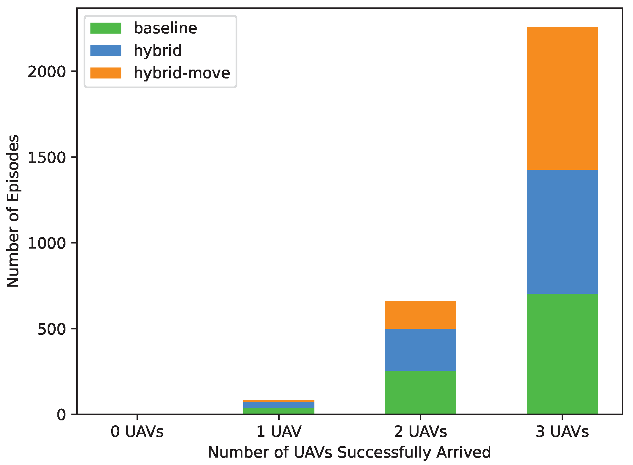
| Methods | 0 UAV | 1 UAV | 2 UAVs | 3 UAVs |
|---|---|---|---|---|
| baseline | 0 | 39 | 256 | 705 |
| hybrid | 0 | 34 | 244 | 722 |
| hybrid-move | 1 | 10 | 160 | 829 |
Disclaimer/Publisher’s Note: The statements, opinions and data contained in all publications are solely those of the individual author(s) and contributor(s) and not of MDPI and/or the editor(s). MDPI and/or the editor(s) disclaim responsibility for any injury to people or property resulting from any ideas, methods, instructions or products referred to in the content. |
© 2024 by the authors. Licensee MDPI, Basel, Switzerland. This article is an open access article distributed under the terms and conditions of the Creative Commons Attribution (CC BY) license (https://creativecommons.org/licenses/by/4.0/).
Share and Cite
Zhao, X.; Yang, R.; Zhong, L.; Hou, Z. Multi-UAV Path Planning and Following Based on Multi-Agent Reinforcement Learning. Drones 2024, 8, 18. https://doi.org/10.3390/drones8010018
Zhao X, Yang R, Zhong L, Hou Z. Multi-UAV Path Planning and Following Based on Multi-Agent Reinforcement Learning. Drones. 2024; 8(1):18. https://doi.org/10.3390/drones8010018
Chicago/Turabian StyleZhao, Xiaoru, Rennong Yang, Liangsheng Zhong, and Zhiwei Hou. 2024. "Multi-UAV Path Planning and Following Based on Multi-Agent Reinforcement Learning" Drones 8, no. 1: 18. https://doi.org/10.3390/drones8010018
APA StyleZhao, X., Yang, R., Zhong, L., & Hou, Z. (2024). Multi-UAV Path Planning and Following Based on Multi-Agent Reinforcement Learning. Drones, 8(1), 18. https://doi.org/10.3390/drones8010018