Article

Optimal Configuration of Heterogeneous Swarm for Cooperative Detection with Minimum DOP Based on Nested Cones

College of Intelligence Science and Technology, National University of Defense Technology, Changsha 410073, China
*
Author to whom correspondence should be addressed.
Drones 2024, 8(1), 11; https://doi.org/10.3390/drones8010011
Submission received: 16 October 2023 / Revised: 29 December 2023 / Accepted: 31 December 2023 / Published: 2 January 2024
(This article belongs to the Special Issue Cooperation of Drones and Other Manned/Unmanned Systems)

Abstract

:
When unmanned platforms perform precise target detection, the configuration of detection nodes will significantly impact accuracy. Aiming to obtain the minimum dilution of precision (DOP), this paper innovatively proposes an optimal detection configuration design method focused on the heterogeneous unmanned cooperative swarm based on the nested cone model. The proposed method first divides the swarm into different groups according to the performances of platforms and then uses a conical nested configuration to arrange the placement of each node independently. The paper considers the problem of the inaccurate prior position of the target and replaces the single-point DOP with the average DOP on the prior region of the target as the optimization objective. Considering the unavoidable positioning errors in engineering practice, this paper provides the optimal configuration of the detection group (DG) and anchor group (AG) in the swarm to reduce the impact caused by positioning errors of detection nodes. We set a certain swarm consisting of 3 types of platforms to design the configuration by simulation experiments and find the optimal parameters for nested cones to realize accurate detection.

1. Introduction

In recent years, with the rapid development of drones and ground unmanned vehicles, a large number of unmanned platforms equipped with complex sensors have been widely used in detection, reconnaissance, and other tasks in various scenarios. Limited by the size, load, or endurance of a single unmanned platform, an unmanned swarm composed of multiple unmanned platforms can better adapt to complex environments and complete tasks [1,2].
In general, according to the composition of the unmanned platform in the swarm, it can be divided into a heterogeneous swarm and a homogeneous swarm. In a homogeneous swarm, the type of unmanned platforms is all the same. Correspondingly, a swarm composed of multiple unmanned platforms with different motion characteristics or detection sensors is called a heterogeneous swarm. Diverse sensors and carrier platforms in heterogeneous swarms give them better capabilities and more approaches when swarms are detected in complex environments [3,4,5].
Cooperative navigation and cooperative detection are important ways to improve the performance of unmanned swarms. Cooperative navigation is to improve the positioning accuracy of other platforms in the swarm by broadcasting observation information within the swarm or relative observation information between platforms. With the sharing of high-precision positioning information provided by nodes with a high-accuracy navigation system, all the nodes in the swarm could obtain higher positioning accuracy [6,7].
Acquisition of an accurate target position is one of the important goals of detection. In a detection swarm, the geometry formed by unmanned platforms has an important impact on target location performance [8,9,10]. Therefore, researchers have explored many optimization strategies for single-target localization problems. Cramer–Rao lower bound (CRLB) and Fisher information matrix (FIM) were used to evaluate estimation performance in articles [11,12], respectively. Various optimality criteria are widely used, such as the D-optimal criterion (maximizing the determinant of FIM) [13] and the A-optimality criterion (minimizing the trajectory of inverse FIM) [14]. The sensor configuration optimization theory based on Fisher information is relatively late in the development of unmanned swarms. Zhang studied the positioning performance of a leader–slave multi-AUV (autonomous underwater vehicle) cooperative positioning system and analyzed the influence of different configurations on the positioning performance through simulation [15]. Fang proposed an optimal configuration estimation method for cooperative positioning based on distance measurement and verified that the optimal formation could obtain better positioning accuracy by analyzing the configurations of single-lead underwater vehicles and double-lead underwater vehicles [16]. In 2023, Bo Xu established a multi-objective AUV three-dimensional cooperative positioning formation optimization model based on angle of arrival (AOA) measurement, used the D-optimal criterion to derive the single-objective and multi-objective evaluation functions of the underwater three-dimensional cooperative positioning system, and used the optimization algorithm to obtain the optimal formation of the cooperative positioning system [17].
In addition to using FIM to establish the objective function for configuration optimization, the method of minimizing DOP to achieve optimal detection configuration has also achieved fruitful results for the single-point detection problem [18,19,20]. The geometric dilution of precision (GDOP) minimization criterion has been widely used in localization configuration optimization. In the study [21], it is considered that in engineering practice, the configuration scheme with practical geometric significance is more practical than the infinite solution. Walker formation has been widely used in the constellation design of satellite positioning [22]. Yang defined a nested conic configuration on the basis of the conic configuration, derived the conditions that the minimum Position Dilution of Precision (PDOP) nested conic configuration should meet, and discussed the method of constructing the minimum GDOP configuration [23,24]. Based on this, Wang has carried out a large number of simulation experiments and discussed and analyzed the GDOP minimization conditions of nested conical configurations with the application background of the ultra-wide band (UWB) positioning system [25].
Currently, most research sets an ideal condition for unmanned swarm detection, which neglects the positioning error in many aspects [26,27]. First, before determining the configuration for precise detection of a single target, the target location needs to be provided by a priori information, which should be imprecise in practice. However, most of the current research does not take into account the effects caused by positioning errors. To solve the problem caused by inaccurate prior positions, Wan Jun seeks the local optimal solution of the GDOP density of each group of buoy combination conical configurations based on the extreme value condition of the minimum PDOP positioning pattern, and then seeks the global optimal solution of the minimum GDOP density from all the candidate buoy combination configurations to achieve the optimal design of underwater positioning formations [28].
In addition, there is also an issue of imprecision in the positioning of each detection node itself. Small platforms such as drones are unable to carry high-precision autonomous navigation equipment limited by cost, size, power, and other limitations. In GNSS interference or rejection environments, their positioning accuracy could be extremely poor, making it difficult to deploy them to the proper placements accurately according to the designed configuration. To deal with the above problems, we employ unmanned ground vehicles (UGVs) equipped with high-precision autonomous navigation systems in the cluster as anchor points and use the principle of collaborative positioning to provide accurate self-position information for the detected UAVs [29].
Cooperative navigation is an important and effective method to improve the performance of unmanned platform swarms, which improves the positioning accuracy of other platforms in the swarm by broadcasting the observation information within the swarm or relative observation information between platforms. With the sharing of high-precision positioning information provided by nodes with a high-accuracy navigation system, all the nodes in the swarm could obtain higher positioning accuracy [30].
Considering practical problems such as positioning errors, this paper focuses on heterogeneous unmanned swarms and fully utilizes their superior performance by utilizing cooperative navigation and detection. The optimal configuration in 3D for minimum DOP would be designed based on nested cones. The main contributions of the article can be summarized as follows:
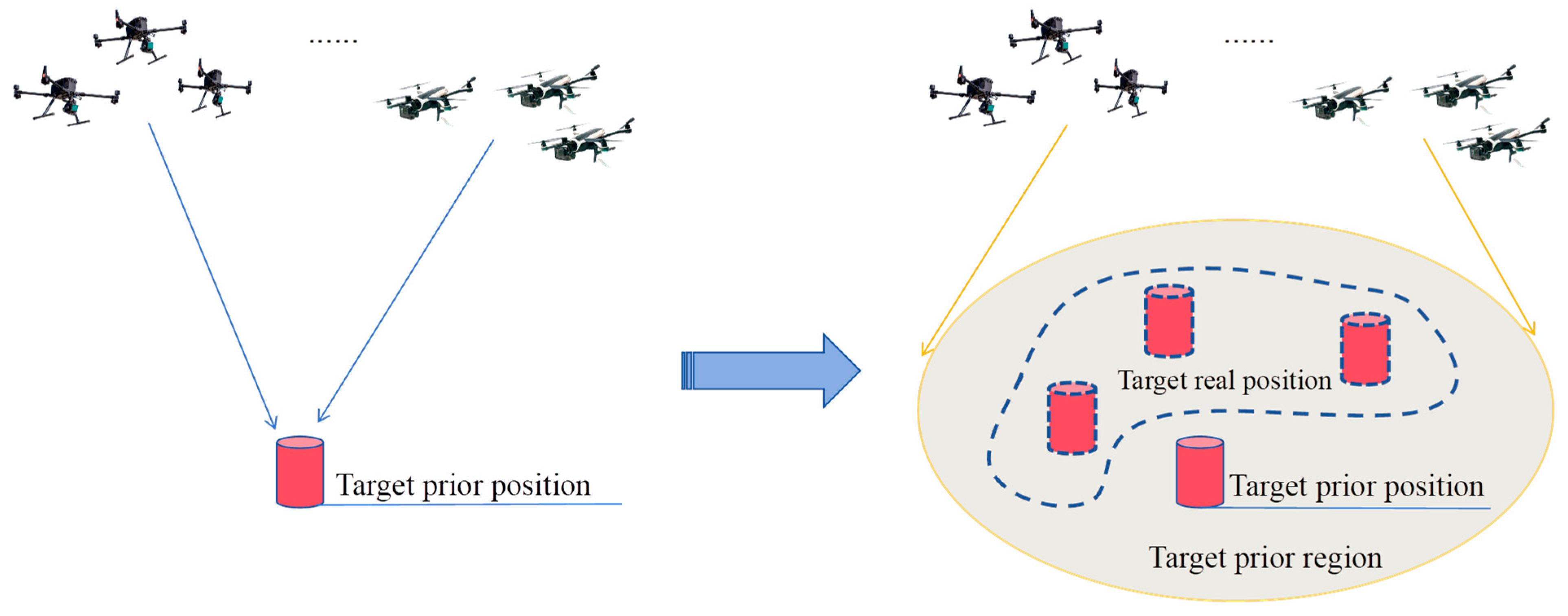
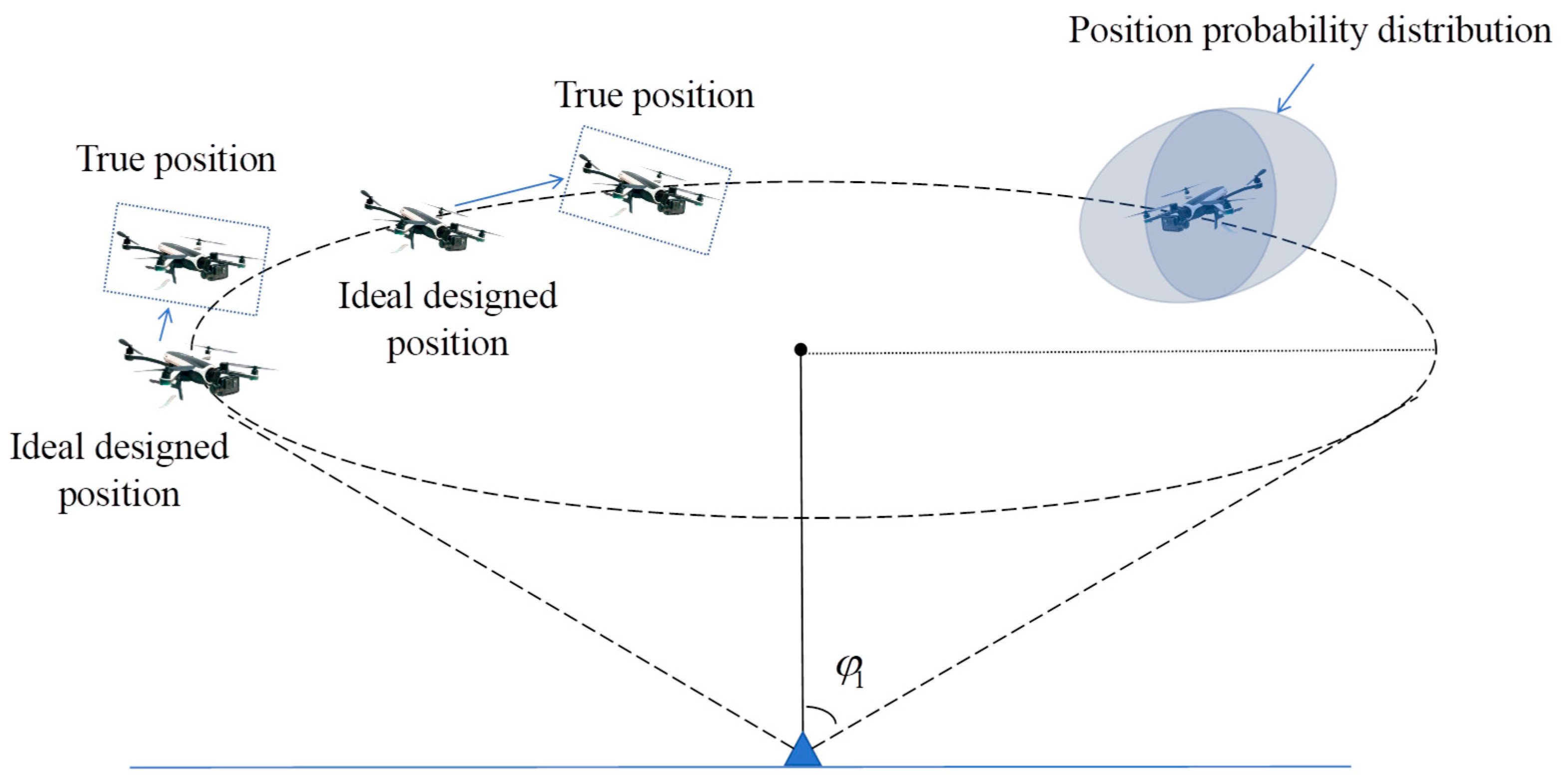
  • In detection tasks, the configuration design based on the target’s prior position relies on the accuracy of prior information. To address the problem of an inaccurate prior position of the target, the optimization objective is transformed from the DOP of the target point to the average DOP of the target area. On this basis, the design problem of the optimal DOP nested cone configuration on the target prior region was studied to ensure that the designed optimal configuration can achieve the minimum DOP value within a certain range on the plane, which avoids the problem of the detection configuration being unable to achieve optimal detection due to inaccurate target prior positions.
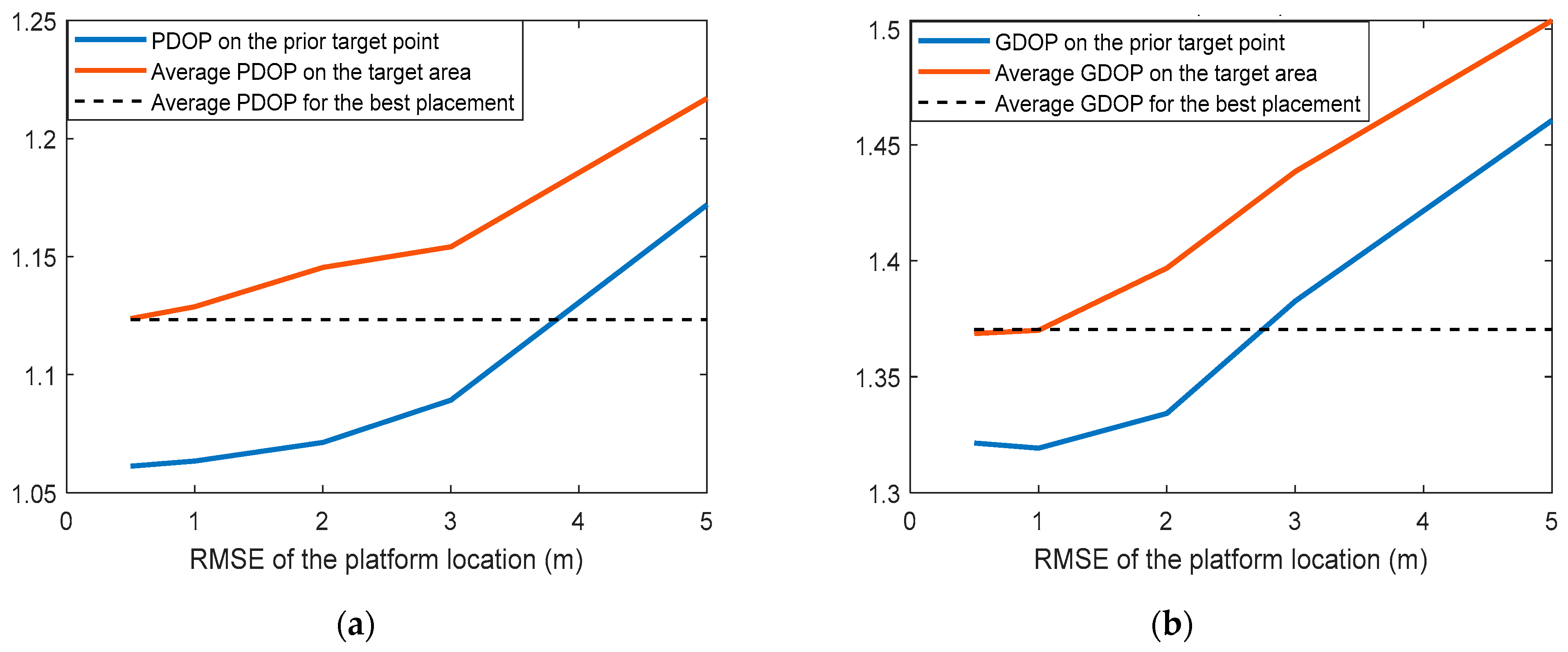
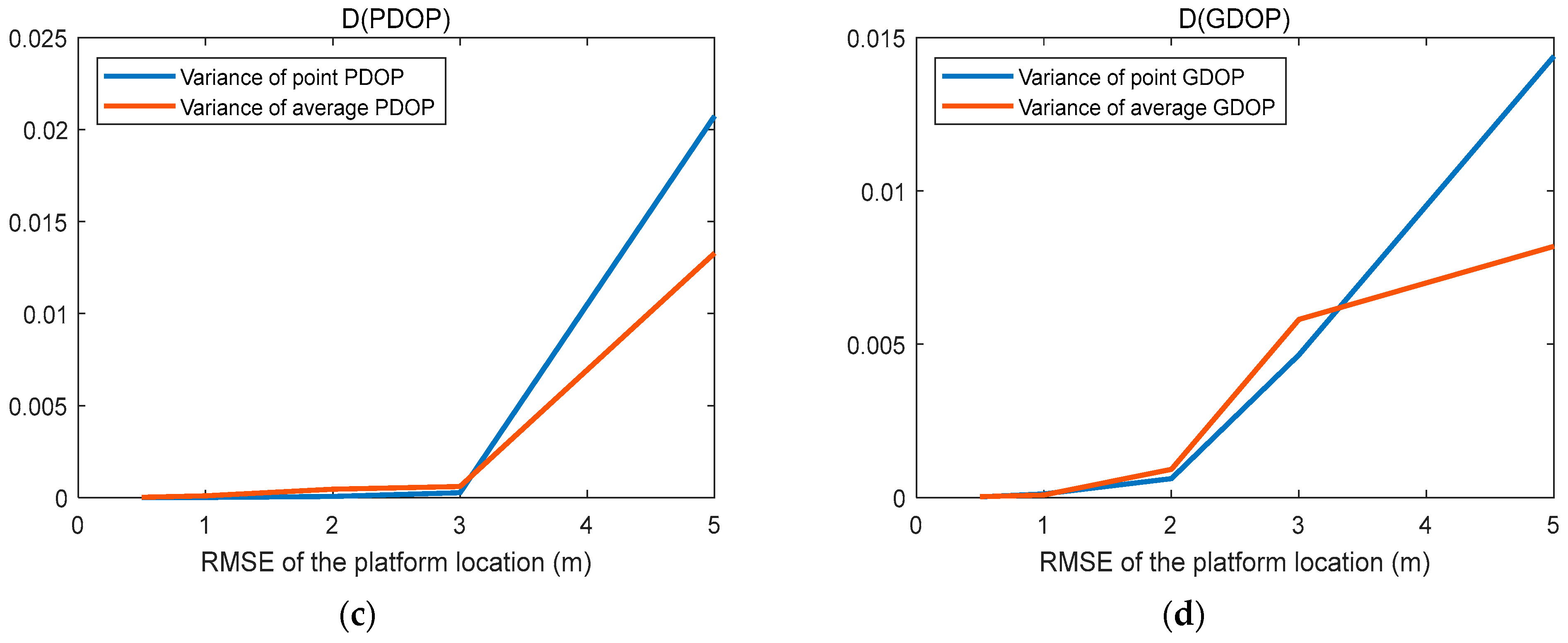
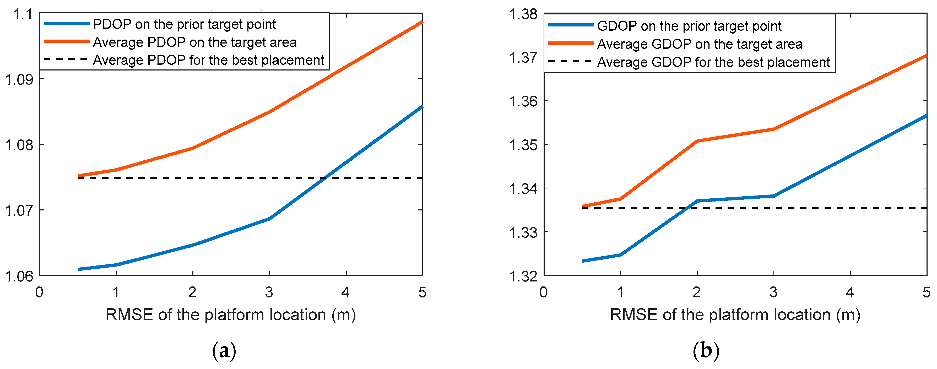
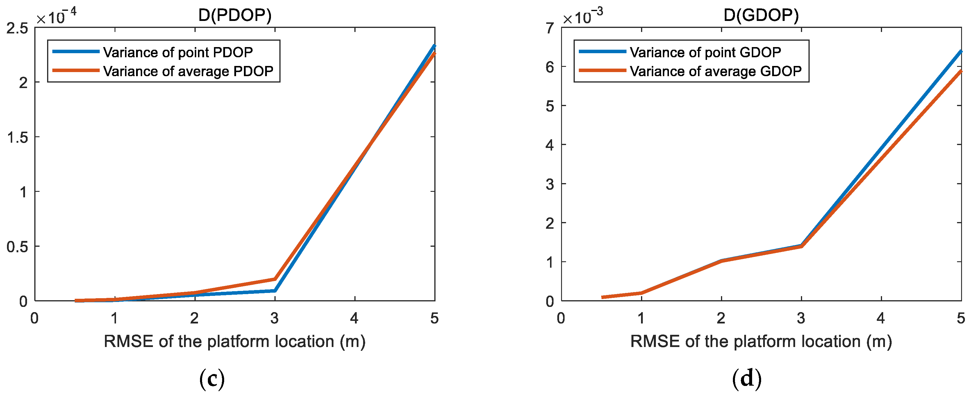
  • Considering that in practical engineering applications, the localization errors caused by the poor self-positioning performance of drones will lead to the inaccuracy of target detection. A large number of simulation experiments were conducted to evaluate the impact of positioning errors on DOP under the optimal DOP configuration, which provides experimental support for the robustness analysis of different 3D optimal configurations against platforms’ localization errors.
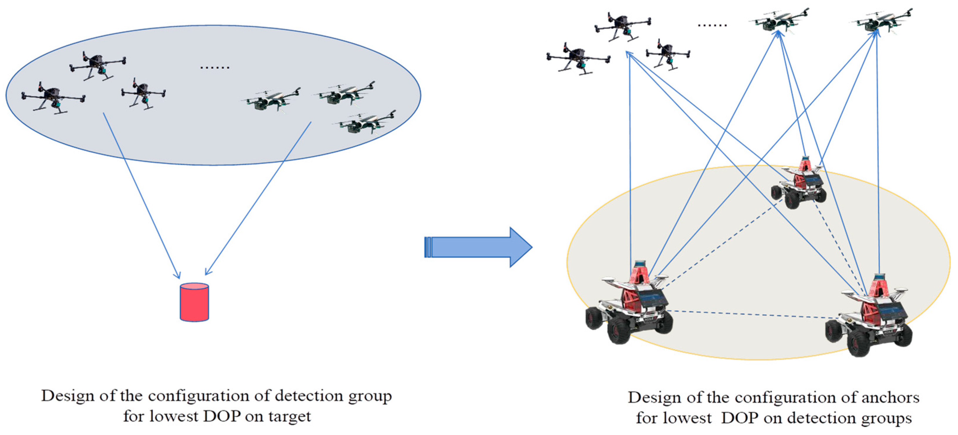
  • Based on the evaluation conclusion drawn from the second work, an AG was designed using UGVs to further reduce the impact of the positioning performance of the detection drones on the detection results. We fully arrange the roles of all nodes in the heterogeneous unmanned swarms and apply cooperative positioning methods to improve the positioning accuracy of nodes in the DG, significantly reducing the self-positioning error of detection nodes and improving the detection accuracy toward targets.
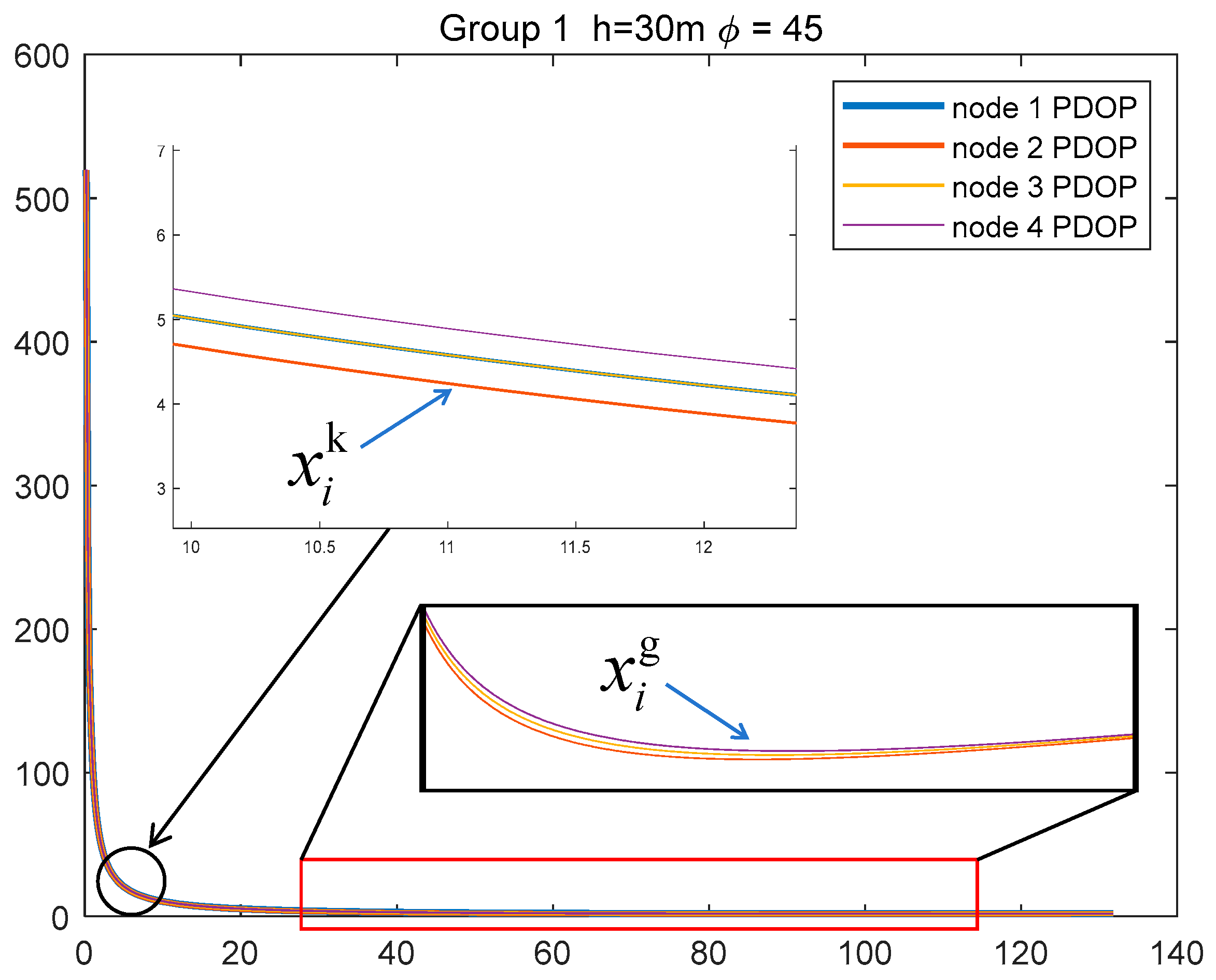
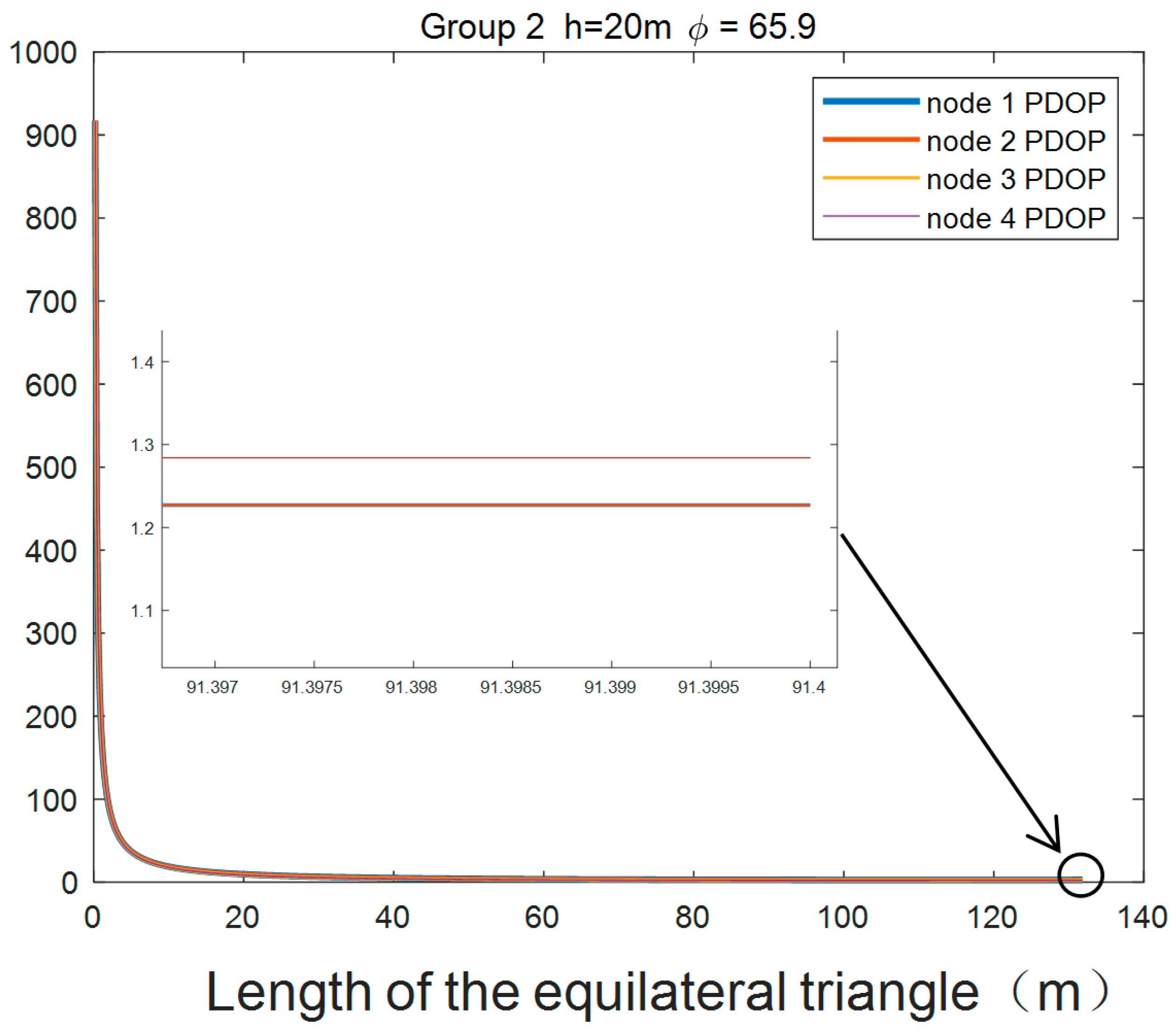
  • To maximize the performance of cooperative navigation for nodes in the DG by optimizing the configuration of the AG, an objective function for minimum DOP for the detection node was established, which was used to design the placement of each anchor point in the AG. By introducing weight coefficients corresponding to each detection node, it is ensured that the configuration design of the AG can remain optimal when facing more complex DGs to optimize detection accuracy.
The following parts of the paper are organized as follows: In Section 2, the design requirements of nested cone optimization are introduced. In Section 3, combining the theory of the second section with the heterogeneous unmanned swarm, a design method for minimum DOP based on nested cone configuration for the cooperative detection of heterogeneous UAVs is proposed. In Section 4, a certain swarm is set up to carry out simulations. The influence on configuration design caused by the errors of the target’s prior position and detection platforms’ location is deeply studied. Based on the results above, we next design an anchor group to enhance the robustness of the configuration dealing with positioning errors and give specific parameters to realize optimization. The results of the comparison simulation are presented in Section 3. The designed detection configuration has greatly improved accuracy compared to random placement. In the final summary, based on the results, we consider the possible practical scenarios and challenges that may be encountered in the next step of application in engineering.

2. Materials and Methods

2.1. Concepts and Algorithms

2.1.1. PDOP and GDOP

DOP is an important indicator of the advantages and disadvantages of the localization configuration, which can reflect the relationship between the measurement error and the localization error, as shown in Equation (1) [31]. e m and e d represent the errors of detection and measurement, respectively. In the case of a certain detection capability of the unmanned nodes, DOP is related to the spatial distribution and number of the nodes for detection. Furthermore, the placement of the platforms in the swarm would affect the accuracy of the detection.
e d = D O P e m
In three-dimensional space, a swarm G n i = { X 1 ,   X 2 , ,   X n } composed of multiple unmanned platforms will constitute a detection configuration G n , 3 , where X i ,   i = 1 ,   2 , ,   n and X i = [ ϕ i , p i ] .
According to the measurement principle of time of flight (TOF) sensors, the pseudo-range observation equation is:
L i = d i + c δ t + ε i i = 1 ,   2 , ,   n
where L i is the pseudo-range measurement between i th detection node X i to the target T = [ x y z ] . In the Equation (2), d i is the true value of Euclidean distance without detection error which could be represented as
d i = ( x i x ) 2 + ( y i y ) 2 + ( z i z ) 2
where δ t is the clock deviation, c is the speed of light in the atmosphere and ε i represents measurement errors introduced by other factors such as multipath effects.
Solving Equation (2) by the least squares method, we could obtain the position coordinates of the target point. Define A i = [ x i x y i y z i z ] 3 × 1 , the least squares solution for positioning a fixed point through the pseudo-range measurement equation can be expressed as:
x = x 0 + ( A T A ) 1 A T L
where x and x 0 is the true position and detecting position of the target.
The positioning error applying this method can be expressed as
σ 2 = tr [ ( J T J ) 1 ] σ 0 2
where σ 0 2 represents the accuracy variance matrix related to measurement sensors. tr is the trace of the matrix. J is the n × 4 Jacobian matrix of the linearized pseudo-range measurement equation. e i = [ x i x y i y z i z ] / d i shown in Figure 1 is the direction cosine from the target point T to the i th detection node. J can be represented as:
J = [ e 1 T e 2 T e n T 1 1 1 ] T
For the detection configuration G n , 3 , the GDOP can be calculated by:
GDOP ( G n , 3 ) = tr [ ( J T J ) 1 ]
PDOP is a special form of GDOP without considering clock deviation. With δ t = 0 , PDOP can be calculated by:
PDOP ( G n , 3 ) = tr [ ( J e T J e ) 1 ]
where J e = [ e 1 T e 2 T e n T ] T and obviously J e is an n × 3 sub-block of matrix J n × 4 which meets J = [ J e k n ] , k n = [ 1 1 1 ] T .

2.1.2. Extremum Condition of DOP Value at Single Point

According to Equation (5), the accuracy of the detection by unmanned platforms is determined by two factors:
The first is the unit weight variance σ . It is determined by factors such as pseudo-range measurement accuracy and localization accuracy of platforms. The other is the DOP related to the parameter covariance matrix, which is determined by the geometric configuration composed of multiple detection platforms.
By calculating ( J T J ) 1 , we have:
( J T J ) 1 = [ ( J e T J e ) 1 + ( J e T J e ) 1 J e T k n ( k n T M k n ) 1 + k n T J e ( J e T J e ) 1 ( J e T J e 1 ) J e T k n ( k n T M k n ) 1 k n T J e ( k n T M k n ) 1 ( k n T M k n ) 1 ]
where M = ( I J e ( J e T J e ) 1 J e T ) .
Using the Gauss Jordan method to solve ( J T J ) 1 , we obtain the equation of minimum GDOP:
GDOP 2 tr ( J e T J e ) 1 + ( k n T M k n ) 1
Based on the Equation (10), we obtain the conditions for minimum DOP.
In two-dimensional space:
min [ GDOP ( G n , 2 ) ] = 2 2 + 1 / n , J e T J e = n 2 I , k n T J e = 0
min [ PDOP ( G n , 2 ) ] = 2 / n , J e T J e = n 2 I
In three-dimensional space:
min [ GDOP ( G n , 3 ) ] = 3 2 + 1 / n , J e T J e = n 3 I , k n T J e = 0
min [ PDOP ( G n , 3 ) ] = 3 / n , J e T J e = n 3 I
In Equations (11)–(14), n represents the number of detection nodes. GDOP ( G ) and PDOP ( G ) means the GDOP and PDOP at the tip of a certain nested cone configuration G , respectively. Obviously, redundant observations will reduce GDOP, thereby reducing detection errors. Whereas, as shown in Figure 2, the improvement of detection accuracy by increasing the number of base stations is quite limited after reaching a certain number since GDOP is inversely proportional to the square root of the number of detection platforms. Compared with PDOP, the minimum GDOP requires k n T J e = 0 additionally. The reason is that the symmetrical placement of the detection platforms will maximize the elimination of errors when it is necessary to consider the impact of clock deviation.

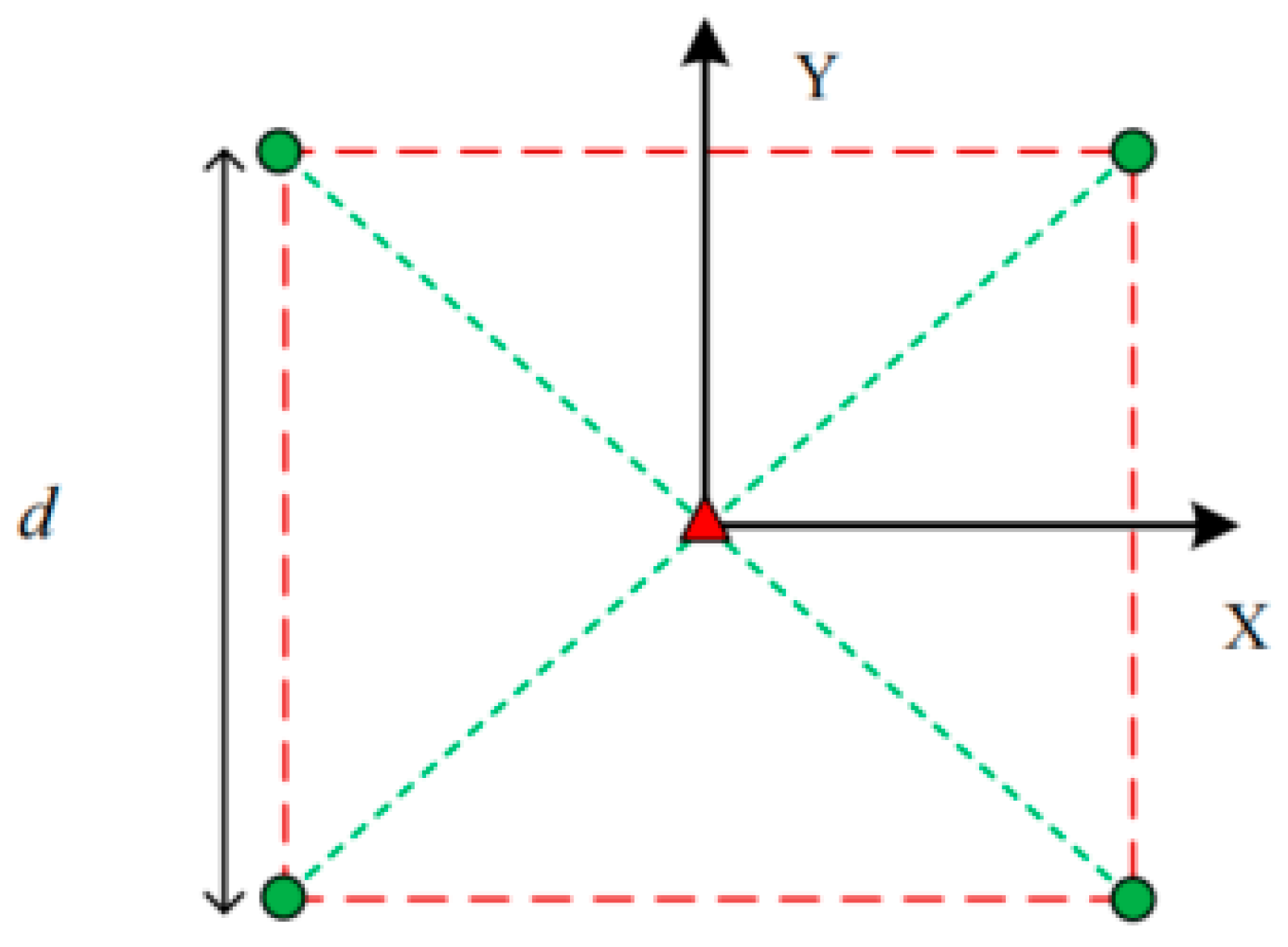
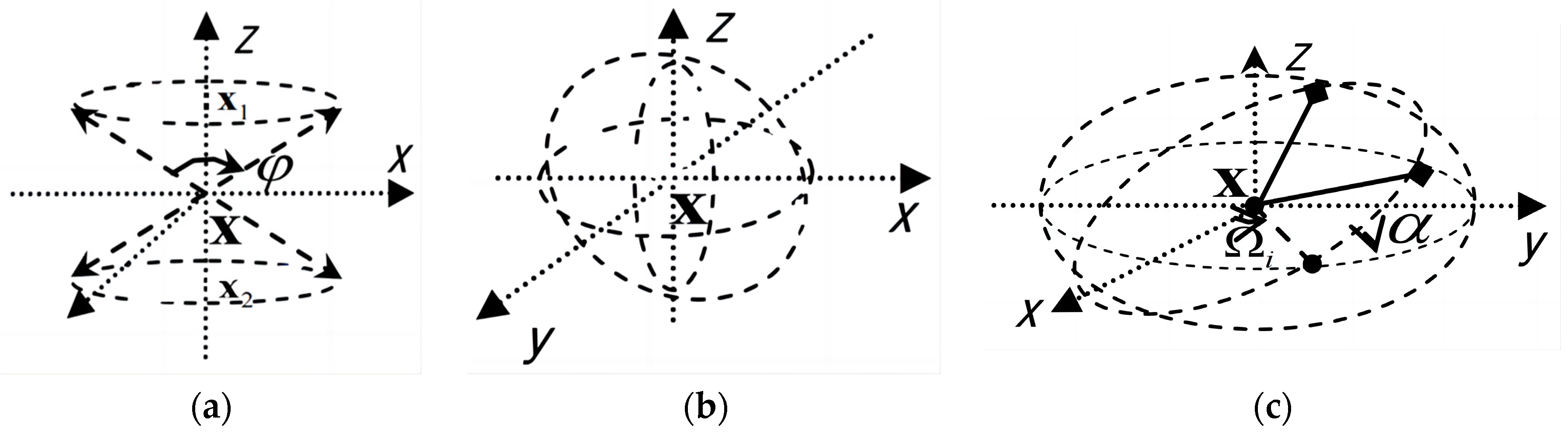
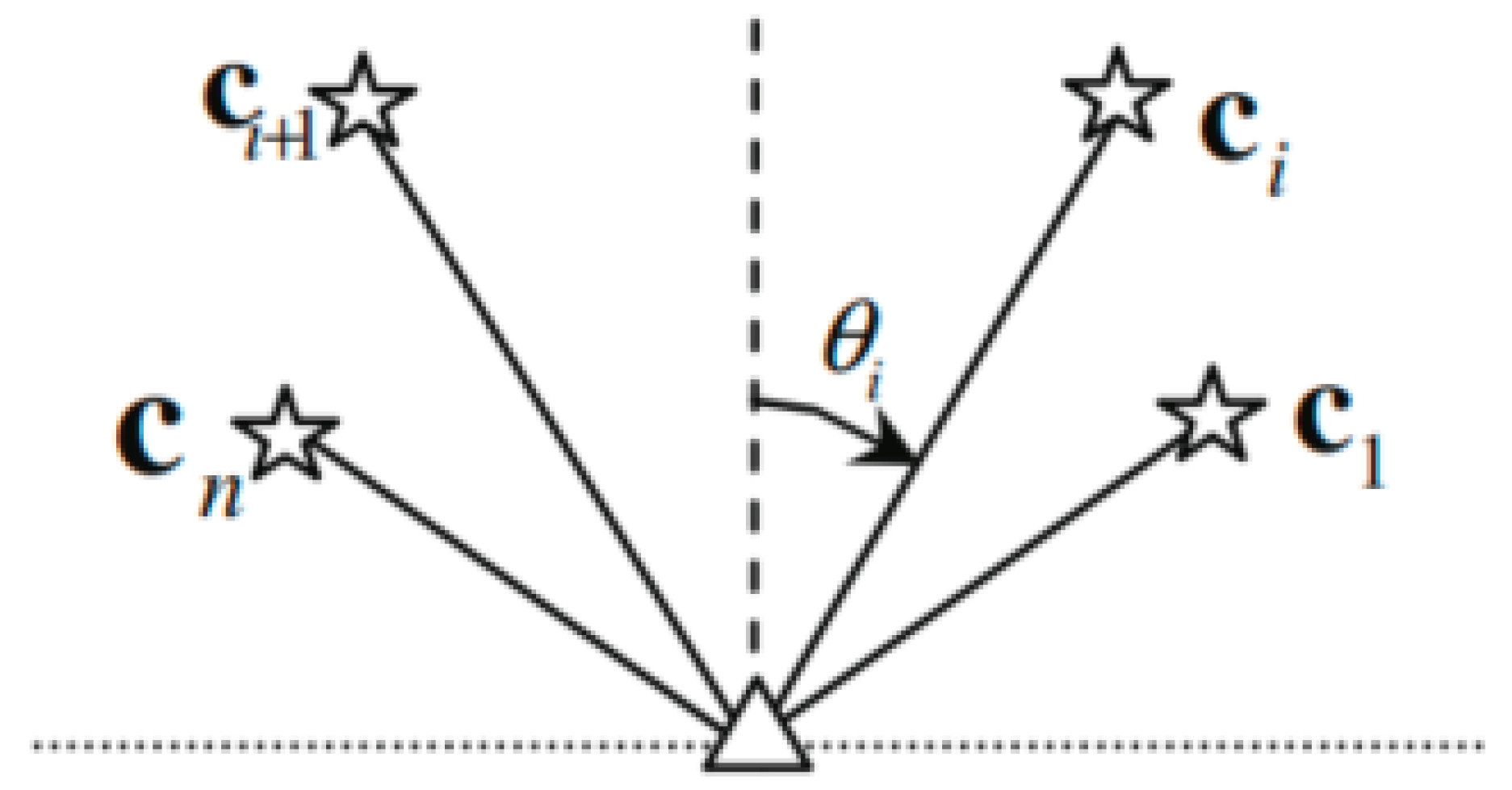
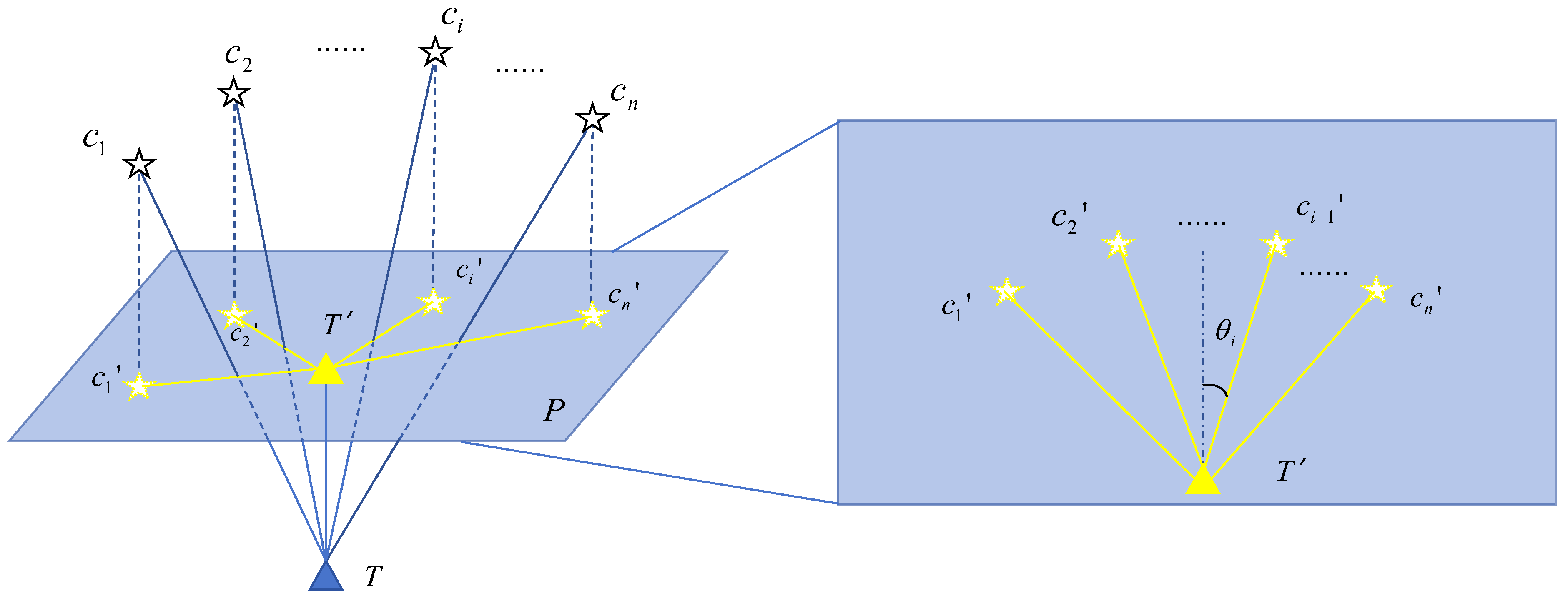
2.1.3. The Configuration of Unmanned Swarm for Minimum DOP at Single Point

Ignoring the motion characteristics of the detection nodes, there can be an infinite number of solutions for min [ DOP ( G n , 3 ) ] based on the minimum DOP condition. The lowest DOP configuration set is defined as:
O n , 3 = { G n , 3 G n , 3 = arg min ( GDOP ( G n , 3 ) ) } P n , 3 = { G n , 3 G n , 3 = arg min ( PDOP ( G n , 3 ) ) }
According to the GDOP minimum condition, various configuration solutions can be obtained in three-dimensional space for point detection, including cone configuration, Cartesian configuration, and Walker configuration, which is shown in Figure 3.
The cone configuration has different forms in 2D and 3D space. In 2D space, the cone has at least one axis of symmetry. As shown in Figure 4, the target and all detection nodes are distributed in a plane. When it comes to 3D space, the cone configurations can be divided into single cone configurations in 3D space and nested cone configurations in 3D space.
As shown in Figure 5a, the vertices of a single cone configuration in 3D space are located at the target point, and all detection nodes are distributed along the edge on the circular bottom of the cone. The coaxial nested cone configuration consists of multiple cone configurations that are coaxial and have the same vertex as the target point to be detected. Except for the vertex and axe, each single cone has an independent parameter.
For the air–ground cooperative detection task for the unmanned swarm, the conditions for forming the optimal detection configuration applying Walker or Cartesian configurations are clearly more stringent due to the limitations of the ground or motion performance of platforms. The nested cone configurations suit the swarms and require all detection nodes to stay on the same horizontal plane much better, which is beneficial for the control of unmanned platforms and the positioning of altitude channels [32]. In addition, the nested cones make it possible to design the placement of different platforms independently, which is more suitable for heterogeneous roles in the swarm to perform different tasks after regrouping. The design of the nested cone configuration would be convenient and intuitive as well. Considering the analysis above, this article adopts a nested cone configuration as the basis for designing the detection configuration for heterogeneous swarms with a minimum DOP.

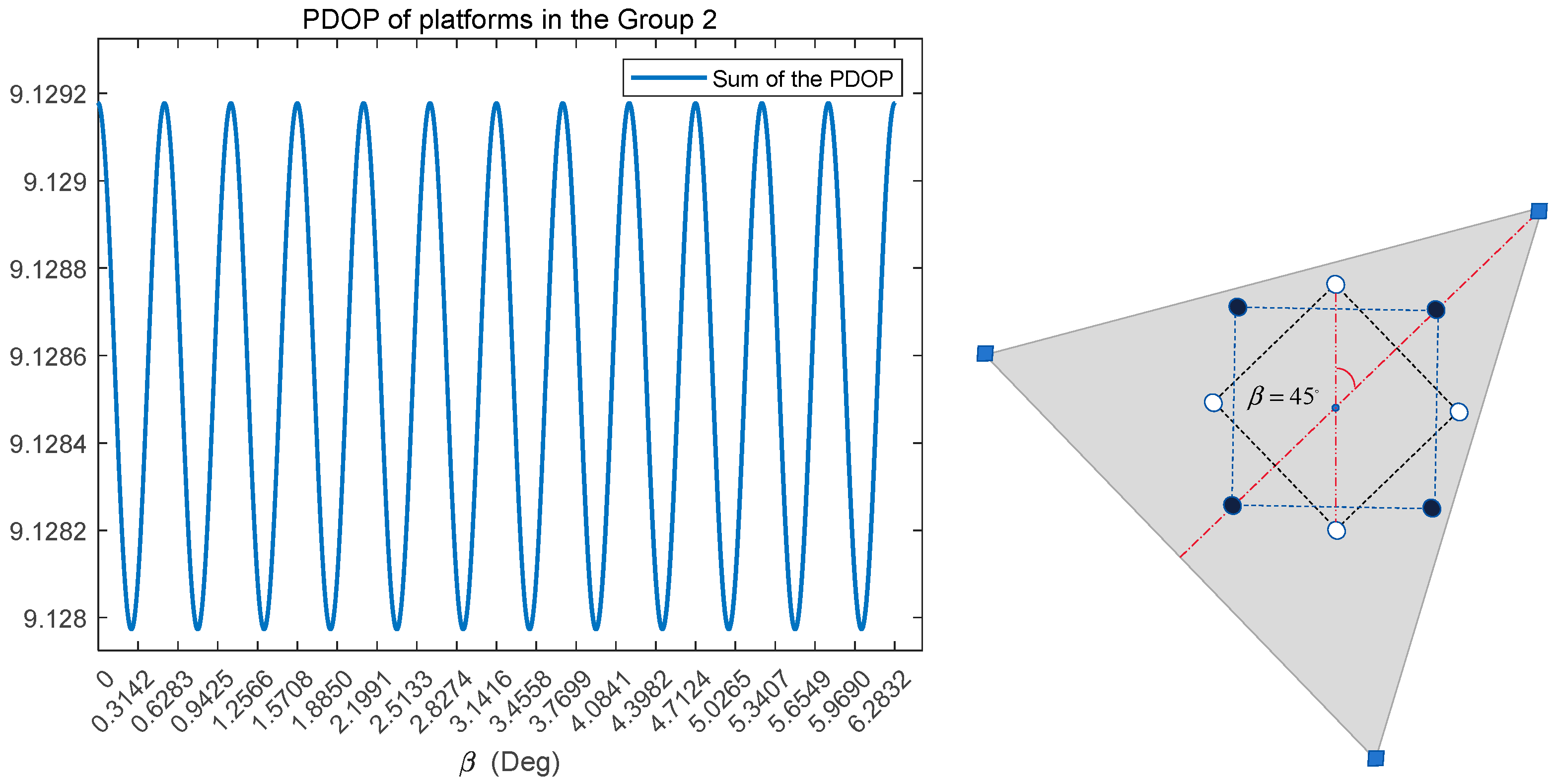
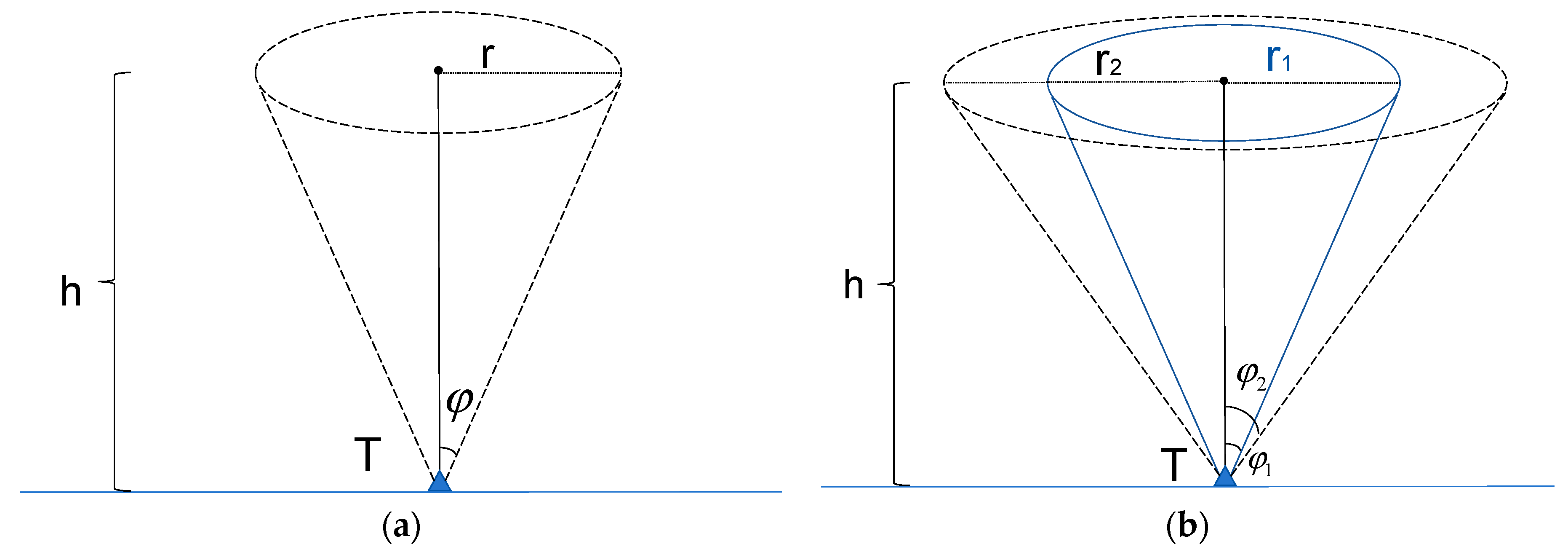
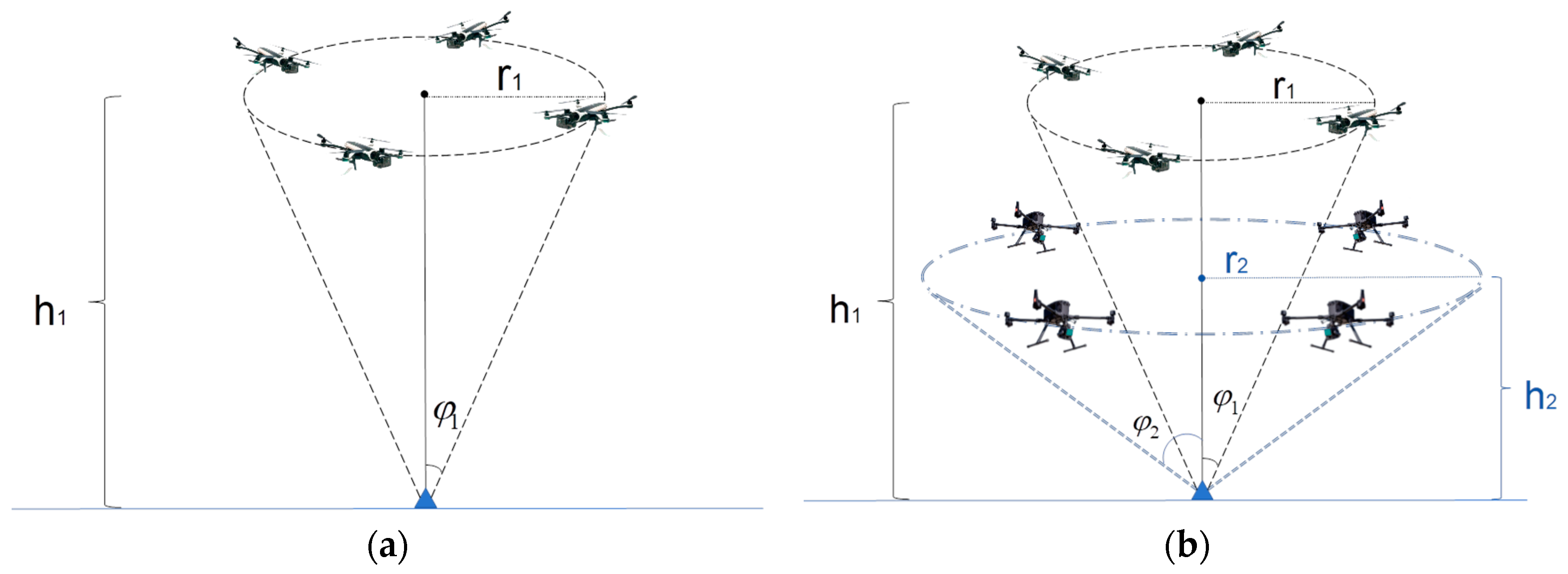
2.1.4. Conditions for Lowest DOP of Nested Cone Configuration

The optimal configurations with the lowest PDOP P n , 3 and configurations with the lowest GDOP O n , 3 should all satisfy the properties below:
  • P n , 3 O n , 3 , i.e., if, G n , 3 P n , 3 , G n , 3 O n , 3 will hold.
  • For any G n , 3 P n , 3 , G n , 3 + G n , 3 I T O n , 3 at the same time. G n , 3 I T represents the new configuration by rotating G n , 3 180° around target point T .
Through the two properties above, it can be inferred that the nested cone configuration has superposition invariance and rotation invariance, which is the theoretical basis for expanding the single cone configuration to the nested cone configuration. When the heterogeneous swarm could be divided into q different groups, and each group would consist of n i ,   i = 1 ,   2 , q platforms, we defined the nested cone configuration of this swarm S q , n as:
G n , 3 = { 1 q G n i , 3 | n = 1 q n i }
where n is the total number of unmanned platforms in the swarm. G n i , 3 is the single cone configuration for each divided group.
To find the optimal nested cone configuration of each detection swarm for minimum GDOP in 3D space, firstly, it is necessary to study the properties of the orthogonal projection perpendicular to the cone axis (referred to as the orthogonal projection) of all detection nodes in 3D cone configuration to the 2D plane. As shown in Figure 6, for a 3D cone configuration, its orthogonal projection on the plane constitutes a 2D cone G n , 2 .
For node placement in 2D space, the projection configuration G n , 2 preserves the basic properties of a 2D cone and has at least one certain axis of symmetry. For the 2D cone in Figure 6, it suits Theorem 1.
Theorem 1.
The condition for obtaining the minimum PDOP at the cone vertex of a planar 2D cone  G n , 2  composed of n detection nodes is:
i = 1 n cos 2 θ i = n 2
At the same time, if and only if
i = 1 n cos θ i = 0
holds, the cone vertex of will obtain the minimum GDOP.
For the design of nested cone configurations, each 2D orthogonal projection of a 3D cone in the nested configuration that satisfies the conditions for the optimal cone is necessary. For G n i , 3 in Equation (16), when the lowest GDOP is obtained at the tip of every cone, Theorem 2 would hold.
Theorem 2.
For the coaxial nested cone  G n , 3 = 1 q G n i , 3 = G n 1 , 3 + G n 2 , 3 + + G n q , 3  in 3D space, if the coning angle  φ i  and the number of platforms ni in the cone satisfy
1 3 1 q n i = 1 q n i cos 2 φ i
The minimum PDOP will be obtained at the common vertex. Similarly, if and only if
i = 1 k n i cos φ i = 0
The minimum GDOP will be obtained as well.

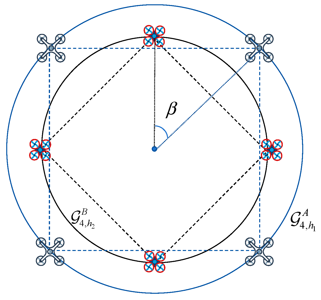
2.2. The Method to Design Coaxial Nested Cone Configuration for Heterogeneous Swarms with Minimum DOP

2.2.1. The Set of the Swarm in the Research

In this section, a specific unmanned swarm consisting of a certain type and number of platforms is set up. In the next research in this paper, we will choose three types of unmanned platforms shown in Figure 7 with different structures and performances to form a swarm. The type and number of platforms are arranged as below:
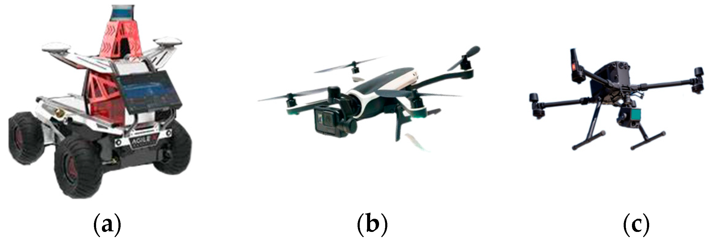
  • Four miniature drones equipped with UWB and range finder.
  • Four large drones equipped with UWB and range finder.
  • Three UGVs equipped with UWB and high-precision inertial navigation system.
It should be noted that although drones of different sizes are equipped with the same sensors in this research, the size of the drones represents more differences between each other, such as cost or performance. For this reason, we regard the drones as different platforms and have divided them into two detection groups. Separating the design of the configuration for each DG can facilitate the control or task management of nodes in the group. At the same time, design potential would be saved for considering different sensors. For the above-mentioned reasons, it is reasonable to arrange heterogeneous unmanned platforms in different cones.

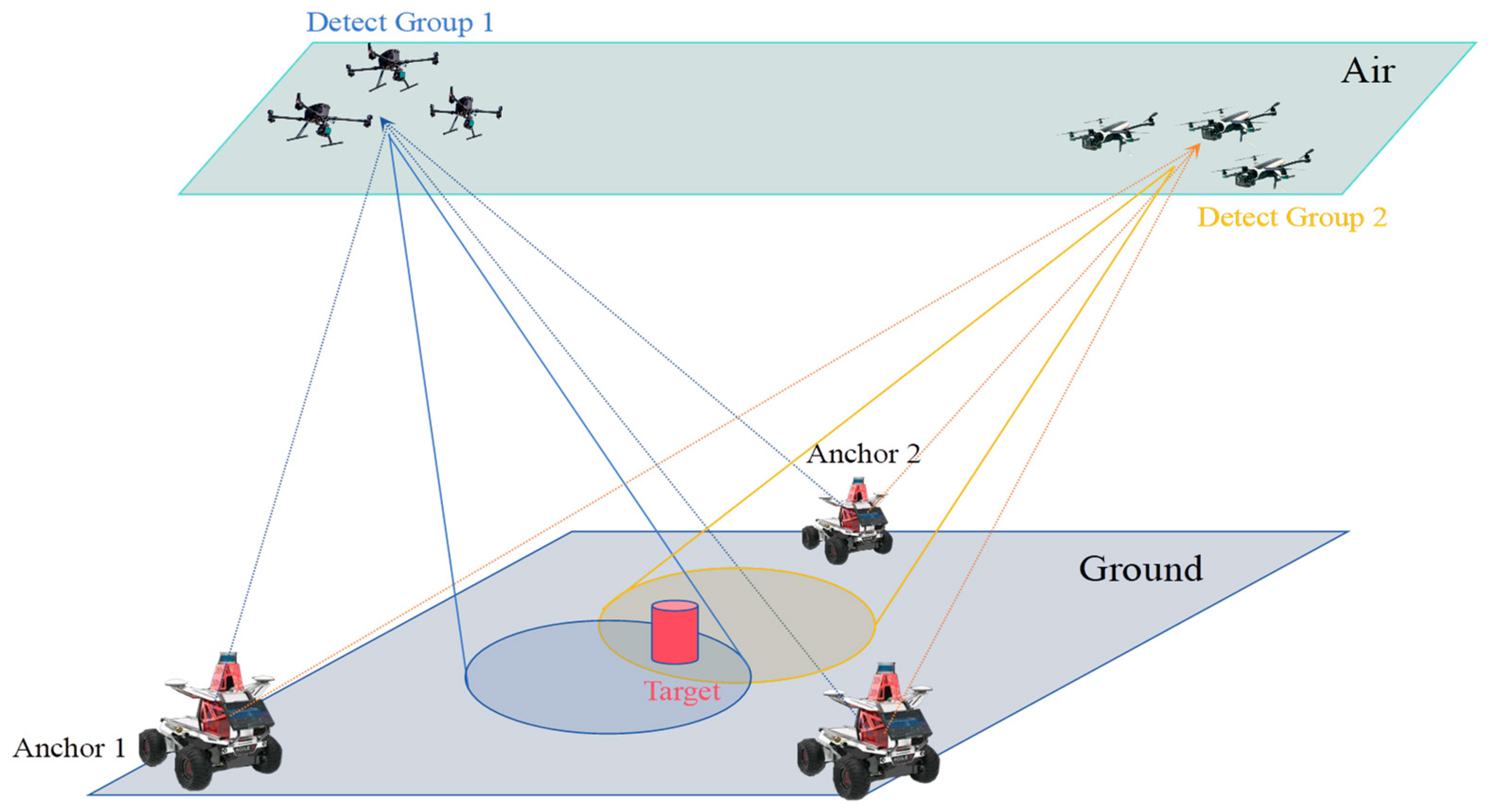
2.2.2. Arrangement for Nodes in the Cooperative Heterogeneous Unmanned Swarm

In order to achieve better positioning or detection results, it is necessary to further subdivide the cooperative swarm into multiple groups for different tasks. As shown in Figure 8, platforms in the swarm can be divided into detection groups and anchor groups (AGs) based on their positioning performance. In general, the platforms in the DGs are able to carry detection sensors such as cameras with high mobility, allow flexible maneuvers, and cost relatively less. Nevertheless, limited by the operating area and the performance of the navigation sensors installed, precise positioning for the detection platforms themselves cannot be achieved. On the contrary, the platforms in the AGs are usually large platforms equipped with high-precision navigation systems that could provide precise positioning in satellite rejection environments. However, the large platforms are not suitable for detecting the target directly due to their high cost and poor mobility. The unmanned platforms in DGs and AGs can collaborate according to their own roles in cooperative detection, which can complete the detection tasks much more accurately, quickly, and safely in the antagonistic area.
Considering the engineering practice, unmanned vehicles with stronger carrying capacity generally play the role of high-precision platforms in AGs, while unmanned aerial vehicles such as drones with better maneuverability and relatively low cost are arranged in DGs. When the drones with detection sensors approach the target for direct detection, the location of each detection platform will be obtained by UWBs equipped as the unmanned ground vehicles (UGVs) perform as anchors. For the above considerations, we divide the cooperative swarm S q , n consisting of n platforms into q different groups as: Anchor groups G A , n i i consisting of n i ,   i = 1 ,   2 q A nodes and detection groups G D , n j j consisting of n j ,   j = 1 ,   2 q D nodes. n i and n j satisfy n = i = 1 q A n i + j = 1 q D n j .
In air–ground cooperative detection, drones in G D , n j j will approach the target as UGVs in G A , n i i stay on the ground. In addition, platforms for the same role might be further grouped according to the differences in the sizes or sensors equipped, if necessary. Fully considering the role differentiation of multiple unmanned platforms in cooperative detection work, this section provides an optimal configuration design method for a cooperative heterogeneous unmanned swarm.
In the method shown in Figure 9, we should set the height of each group during the detection process first based on specific tasks, platform performance, and other prerequisite factors after selecting the target and regrouping the swarm. The next step is the design for the configuration of different groups. Clearly, the design of the configuration for each group in different cones is independent of each other. This characteristic makes it simpler to complete the optimal configuration design of the entire swarm. Although the configuration of the DGs has been fixed, we only need to adjust the AG’s configuration to achieve optimal positioning for all detection nodes in the DGs. As shown in Figure 10, the design for the G D , n j j aims to achieve the minimum DOP at the undetermined target point. Whereas the design of G A , n i i is to achieve the optimal positioning effect at the location of the deployed detection nodes. In general, we assume the platforms in one group perform in the model with the same parameters and accuracy.
The design of each group is all based on the theorems in Section 2. According to Theorem 2, the orthogonal projection G n i , 2 i to the configuration G n i , 3 i placed by G D , n j j should be designed properly first. After this step, the relative position of all nodes in the same group would be fixed with the height being set. In Theorem 1, G n i , 2 i should usually be an axisymmetric figure centered on the target, so only the relative angles θ i between the target and platforms need to calculate. With the G n i , 2 i designed, we only need to determine the coning angle φ i of each cone, which could then fix G n i , 3 i . At this point, it will be noted that if the relative position between different groups needs to be determined, an extra parameter is also required, which is the relative angle β i between the 2D projections of different groups. In a certain swarm, once the θ i , φ i , and β i have been set, the coaxial nested cone configuration for DGs would be fixed. A classic single cone detection configuration G 4 , 3 and a nested cone configuration G 4 , 3 1 + G 4 , 3 2 placed by G D , 4 1 and G D , 4 2 are shown in Figure 11.
The design of other cones for AGs is the last step after achieving the minimum DOP at the target point using the nested cone configuration. The configuration design for the AGs is similar to that of the DGs, but the difference is that the nodes in Anchor have to stay on the ground when we set UGVs as platforms. Although the height of AGs is set to 0 and the cones degenerate into circles on the plane, we still define the configuration of AGs as G n i , 3 i , so the β i and θ i also need to be determined. The difference comes up because the configuration of AGs focuses on DOP on not only one point but also i = j q D n j nodes in G D , n j j , which would be influenced by the size of configuration. Thus, the r i for the ground circle needs to be determined to complete an optimal configuration.
In order to focus our research on structuring the optimal configuration for cooperative detection, we make the following assumptions about the detection process in a heterogeneous unmanned swarm:
  • The communication between all nodes in the swarm is completely smooth, and there is no multipath or clutter in time of arrival (TOA) measurements.
  • Each node has a unique identification, i.e., the problem of data association has been solved, and each measurement is correctly associated with the correct platform, which solves.
  • The UGVs in G A , n i i are equipped with high-precision positioning equipment, which makes it possible to keep the positioning results in the local geographic coordinate system that will not diverge and remain within a certain error.
  • The target is on the ground plane with 0 altitude.

3. Results

As mentioned above, we set 8 drones in 2 DGs and regard 3 UGVs as 3 anchors in one AG to form a swarm. Based on the configuration optimization strategy designed, we comprehensively consider various practical problems encountered in cooperative navigation, focusing on the impact of positioning errors on optimization decisions. In the engineering practice of cooperative navigation, unprecise localization will bring up many problems involved with random variables. In this section, simulation experiments are conducted to visually demonstrate the impact of configuration design parameters on DOP using function figures. Based on the results, suggestions for designing optimal detection configurations are proposed for air–ground unmanned swarms to facilitate making decisions when facing a complex environment.

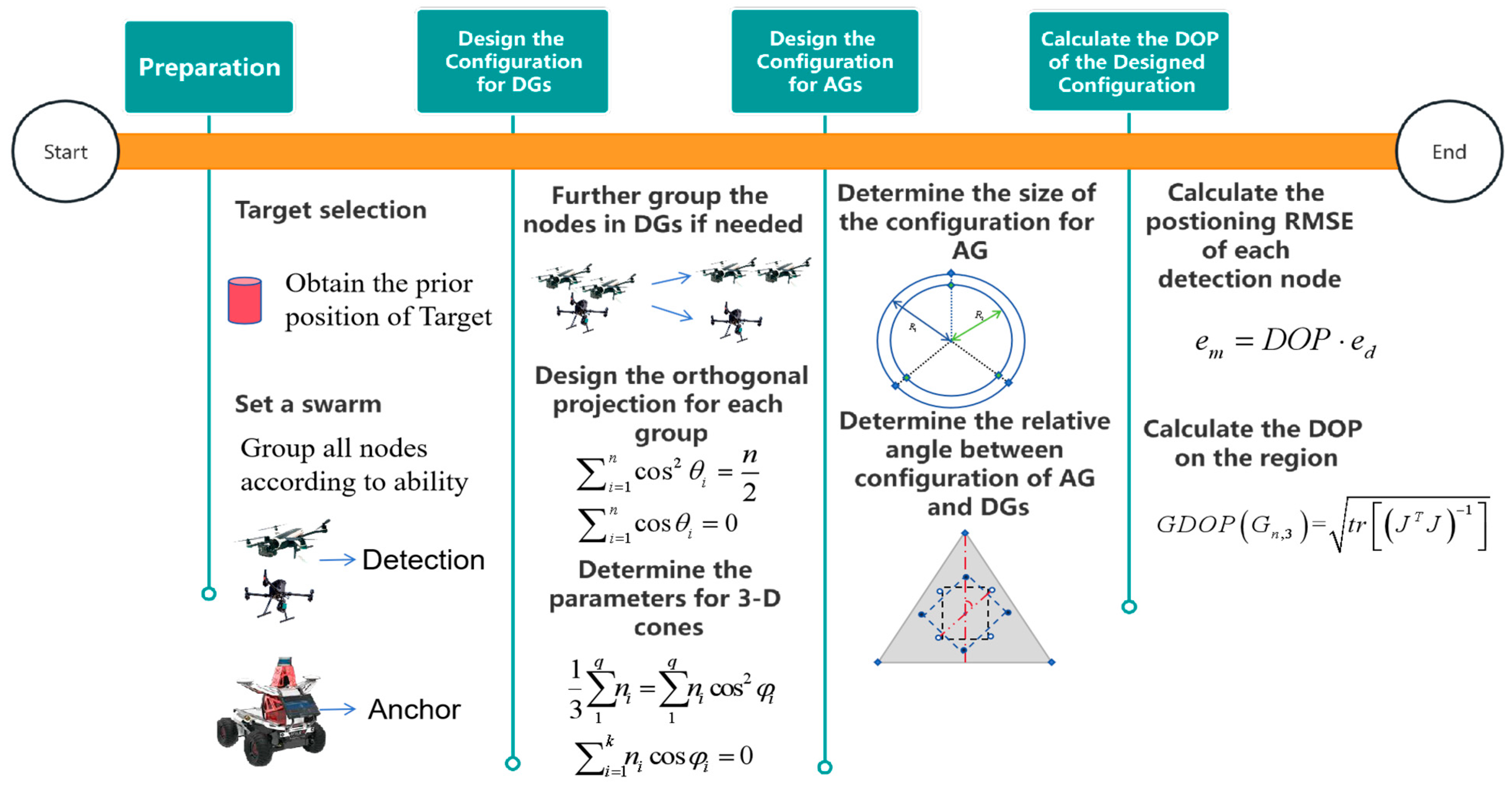
3.1. The Design of Configuration for DGs

3.1.1. Design of Configuration for Minimum DOP at the Target Point

Define the 2 DGs as G 4 , h D 1 D 1 and G 4 , h D 2 D 2 . According to Theorem 2, we need to first design the orthogonal projection of the configuration of G 4 , h D 1 D 1 and G 4 , h D 2 D 2 . For G 4 , h i i consisting of 4 nodes, we need the θ i satisfy:
i = 1 4 cos 2 θ i = 4 2
at the same time,
cos θ 1 + cos θ 2 + cos θ 3 + cos θ 4 = 0
In fact, when more than 4 platforms exist in the DG, the equations for minimum GDOP are underdetermined, i.e., the solutions for Equations (21) and (22) are infinite. When considering the field of view of the sensor, it is generally considered to have θ 1 = θ 2 ,   θ 3 = θ 4 . So Equation (21) becomes:
i = 1 4 cos 2 θ i = 4 2 cos 2 θ 1 + cos 2 θ 2 = 1
with
cos θ 1 + cos θ 2 = cos θ 3 + cos θ 4 = 0
The solution for θ i is θ 1 = θ 2 = π 4 ,   θ 3 = cos θ 4 = 3 π 4 . Obviously, when there are 4 platforms with equal accuracy forming a detection configuration, if and only if the configuration G 4 , 2 is square with its center at the target point exactly, G 4 , 2 O 4 , 2 , the GDOP would obtain the theoretical minimum at the target.
Furthermore, the orthogonal projection of configuration of G 4 , h D 1 D 1 and G 4 , h D 2 D 2 should be placed as shown in Figure 12. In this placement, the G 8 , 3 = 1 q G n i , 3 i = G 4 , 3 1 + G 4 , 3 2 formed by 2 DGs would make it possible that the GDOP or PDOP reaches a minimum at the tip of the nested cone.
Large drones could carry heavier and more precise detection sensors, so making them further away from the target would be a decent strategy. Set the height of DG with small drones, and that for another group with large drones is h 2 . The condition for obtaining the minimum PDOP is:
cos 2 φ 1 + cos 2 φ 2 = 2 3 h 1 2 r 1 2 + h 1 2 + h 2 2 r 2 2 + h 2 2 = 2 3
where φ 1 and φ 2 represent the coning angle of G 4 , 3 1 and G 4 , 3 2 . r 1 and r 2 are the radius of two cones.
In addition, if and only if 4 cos φ 1 + 4 cos φ 2 = 0 , minimum GDOP could be obtained at the tip of the detection configuration G 8 , 3 . However, it is impossible to meet φ π 2 in the air–ground detection application. Under the limitation of the detection cut-off angle, no configuration can satisfy the requirements of Theorem 2. Thus, we introduce the nonlinear programming problems for minimization as below:
{ min   f ( φ 1 , φ 2 ) = cos φ 1 + cos φ 2 s . t .   cos 2 φ 1 + cos 2 φ 2 = 2 3
Under the constraints of Equation (26), the value approximates a parabolic curve, as shown in Figure 13. The value would reach its maximum when φ 1 = φ 2 54.76 ° and reach a minimum of 0.8165 when φ 1 = 35.26 ° , φ 2 = 90 ° . In this configuration, the PDOP at the target point would obtain the theoretical minimum of 1.06 and the GDOP would reach its practice minimum of 1.225, which increases by about 9.54% compared with the theoretical minimum GDOP. Significantly, it is generally considered to maintain a cut-off angle due to the need for drones to fly at a certain altitude. In practice, the cut-off angle would be affected by multiple factors, so in this section, we ignore this problem and keep φ 1 = 35.26 ° , φ 2 = 90 ° as the parameter of the nested cone for further research.
As the parameters for the configuration are fixed, the orthogonal projection of the placement of G 4 , h D 1 D 1 and G 4 , h D 2 D 2 is shown in Figure 14. In this figure, the relative angle β between two DGs is much clearer.
According to Equations (5) and (6), the DOP at the target point located at the tip of the cone would become fixed constants no matter how β between single cones changes. The results are shown in Figure 15. On the contrary, GDOP/PDOP is more sensitive to changes in relative angle on the plane near to the cone tip.

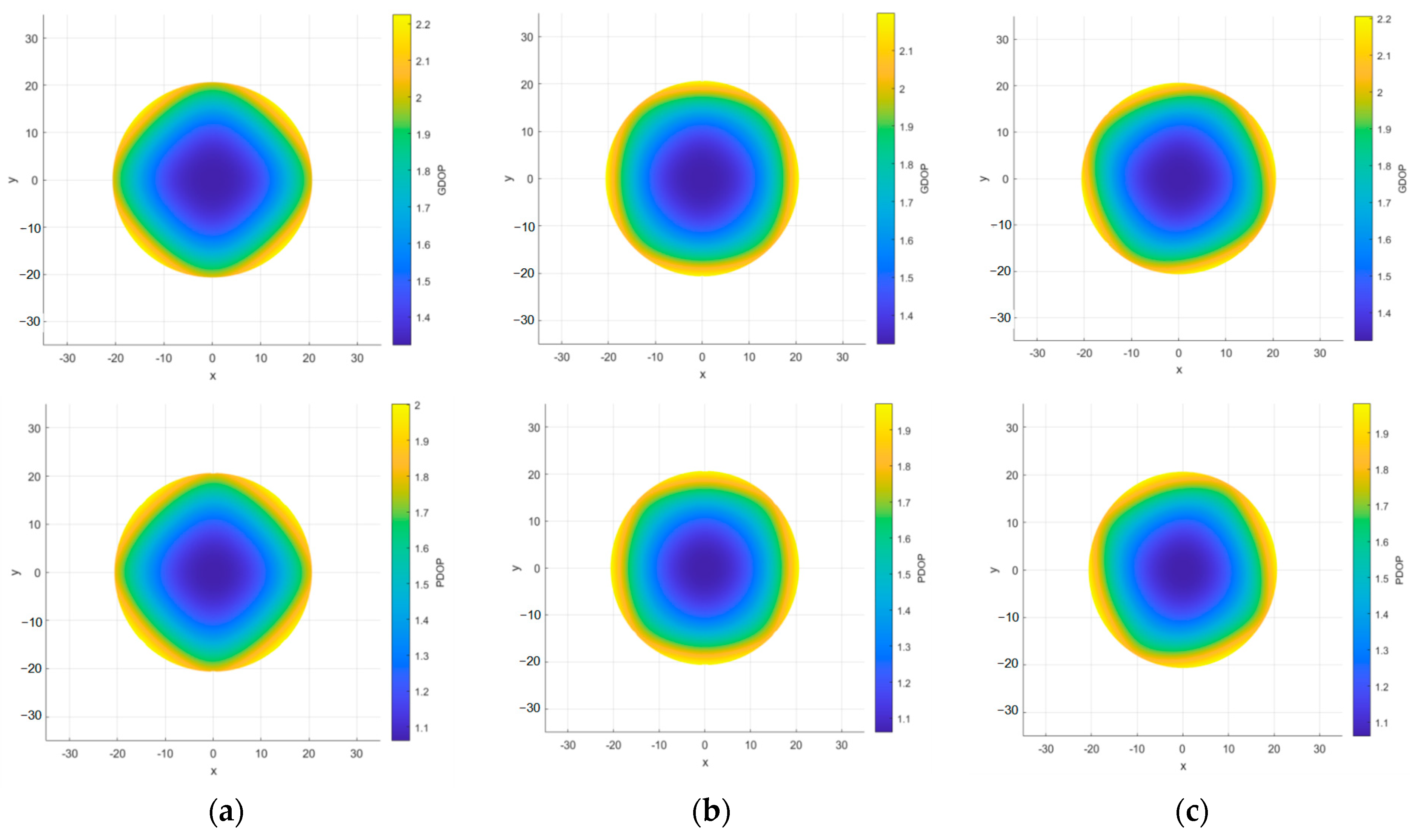
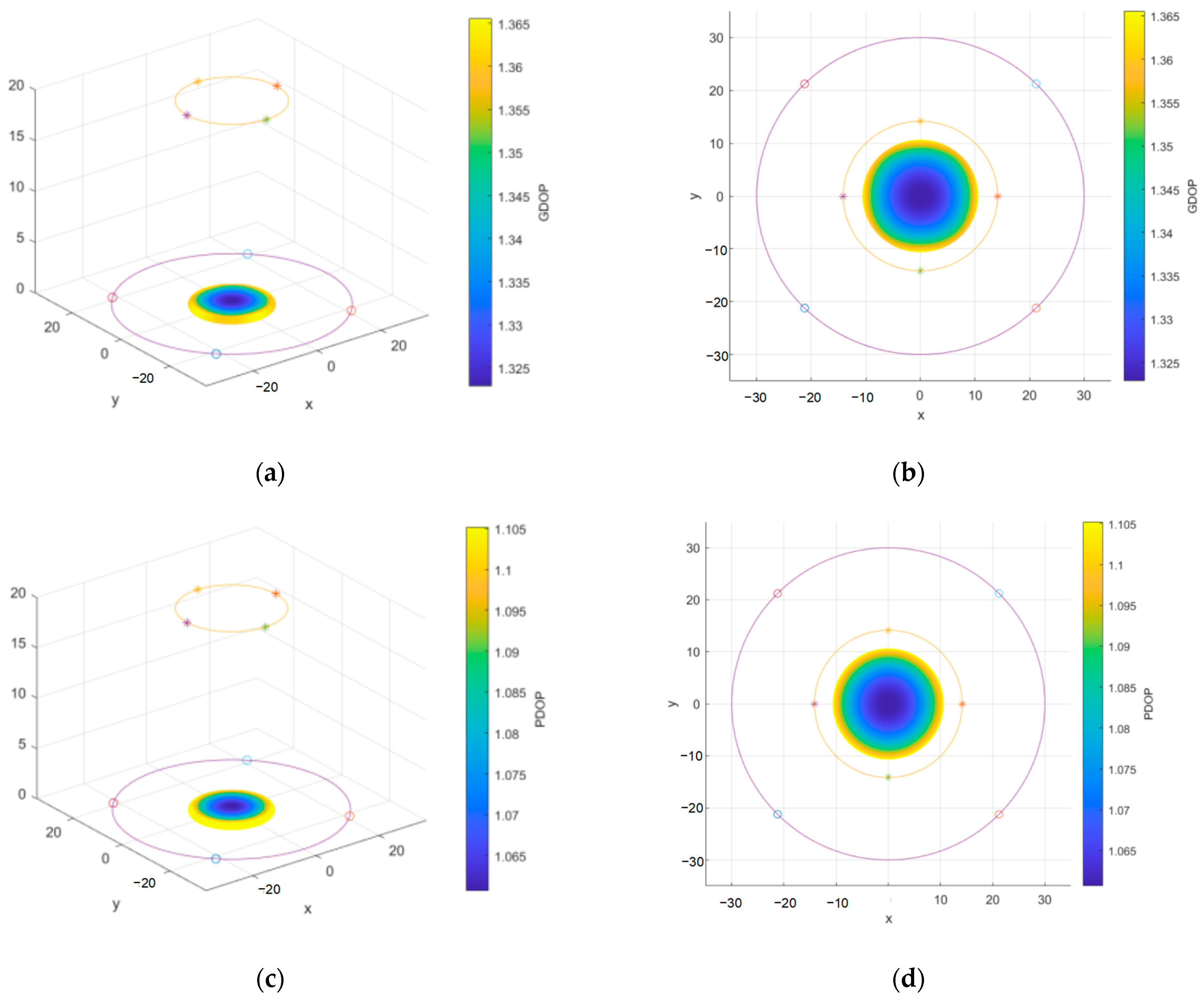
3.1.2. Design of Configuration for Minimum DOP on the Prior Target Region

In Section 3.1.1, we assume that the vertices of the nested cone formation are located at the target, which has inaccurate prior position information in practical terms. As shown in Figure 16, it is necessary to change the design specification of the optimal configuration from the DOP at the cone tip to a weighted average DOP value oriented towards a region, considering that DOP varies significantly in the plane far from the cone tip, which might be influenced by more factors.
Generally, it is believed that the detection error of ground targets satisfies the Gaussian distribution if the prior information is sufficiently reliable. It can be considered that the actual position of the target to be detected should be distributed within a circle with a certain radius centered on the target prior position, which we define as the target prior region.
Set the height for 2 DGs as h 1 = 30   m and h 2 = 20   m , then we obtain the distribution map of the DOP value in the target prior region shown in Figure 17. The consensus has been that the DOP will become lower as it approaches the cone tip. However, in the middle of each distribution map, the distribution is quite similar, so it is hard to determine which β could lead to a lower DOP.
In order to evaluate the accuracy of the target prior region, we apply differentiation to divide the ground. In the process of satellite configuration design [33], the Earth’s surface is divided into 5120 triangular units, and the average GDOP/PDOP is defined as the final evaluation indicator as Equation (27).
E ( GDOP g r o u n d ) = i = 1 n GDOP ( p i ) / n E ( PDOP g r o u n d ) = i = 1 n PDOP ( p i ) / n
GDOP ( p i ) and PDOP ( p i ) represents the GDOP/PDOP of the divided ground, which is centered at the point p i . Employing the above method of differentiating the ground near the target, the geoid can be approximated as a plane because the target prior region is much smaller than the Earth’s surface. As shown in Figure 18, the target prior region could be a planar circle with its radius R max = 10   m . The size of the radius reflects the confidence level of prior information. Divide the plane circle into 200 concentric circles from the inside out, keeping the difference Δ d in radius between adjacent concentric circles at 0.5 m, which divides the area into 200 equally wide rings. Then we use an equilateral triangle with a height of Δ d to fill the rings. According to the differentiation method above, we obtain:
k i = 2 l i 3 Δ d + 2 l i 1 3 Δ d = 4 π R i 3 Δ d + 4 π R i 1 3 Δ d k = i = 1 200 k i 2175
Taking the central DOP of an equilateral triangle as the DOP of the entire triangle, then Equation (29) becomes:
E ( GDOP g r o u n d ) = i = 1 20 j = 1 k i GDOP ( p i , j ) S i , j S E ( PDOP g r o u n d ) = i = 1 20 j = 1 k i PDOP ( p i , j ) S i , j S
where S i , j represents the area of the j th triangle on the ith ring, which is centered at p i , j , and S is the total area of the prior target region.
According to Equation (29), we studied the variation of DOP in the prior target region near the cone tip with the relative angle β . The PDOP and GDOP maintain the same trend of change, and both reach their minimum at β = 45 ° with symmetric distribution, as shown in Figure 19.
Fix the parameter β = 45 ° , we note that the GDOP and PDOP would change with the change in the height of DG. The average DOP would reach a lower value when the height or radius of the cone increases, which indicates that the average DOP will be influenced by more parameters. For these reasons, more simulation experiments were conducted on other combinations of cone angles with cos 2 φ 1 + cos 2 φ 2 = 2 3 , and the results are presented in Table 1.
The results obtained confirms two vital corollaries:
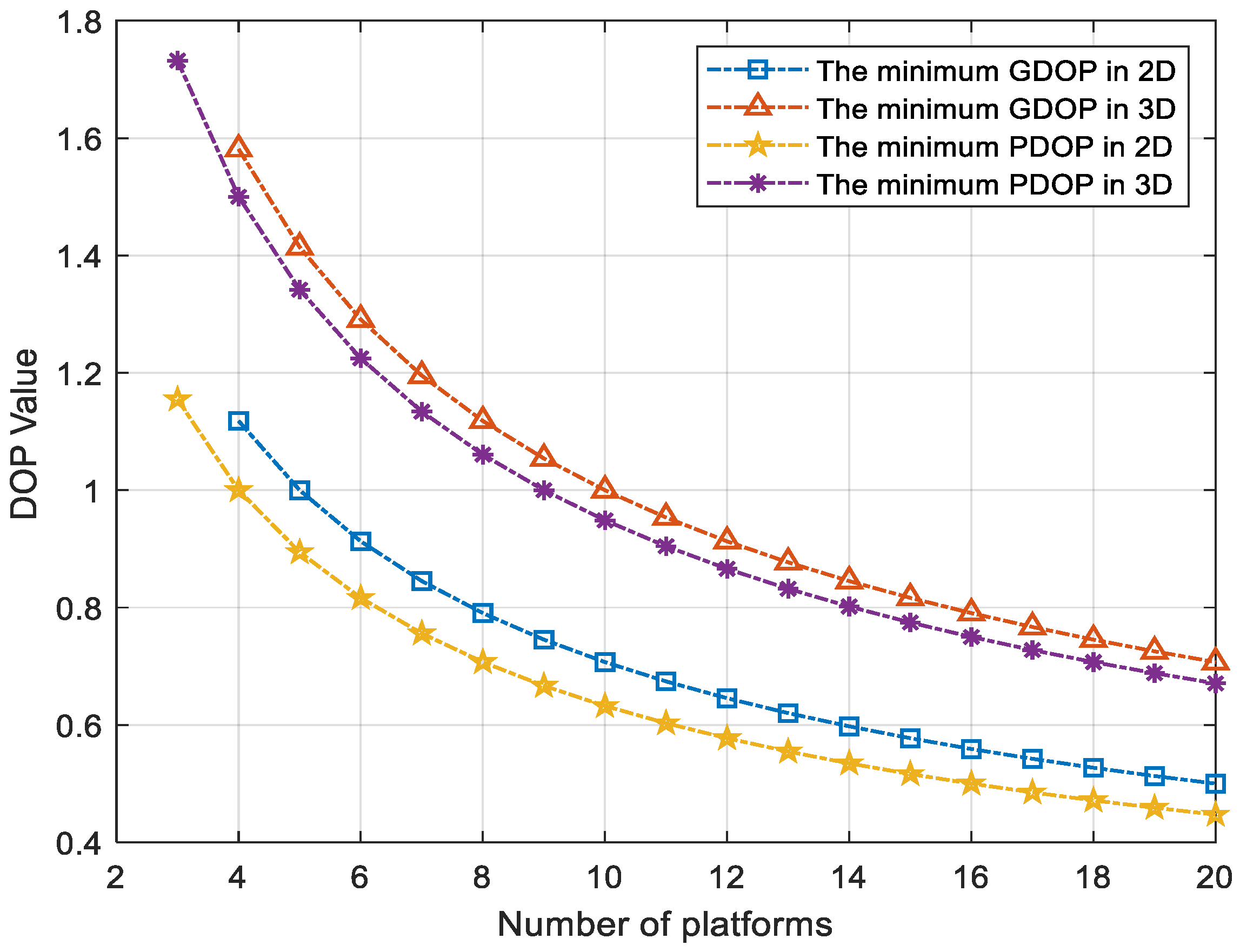
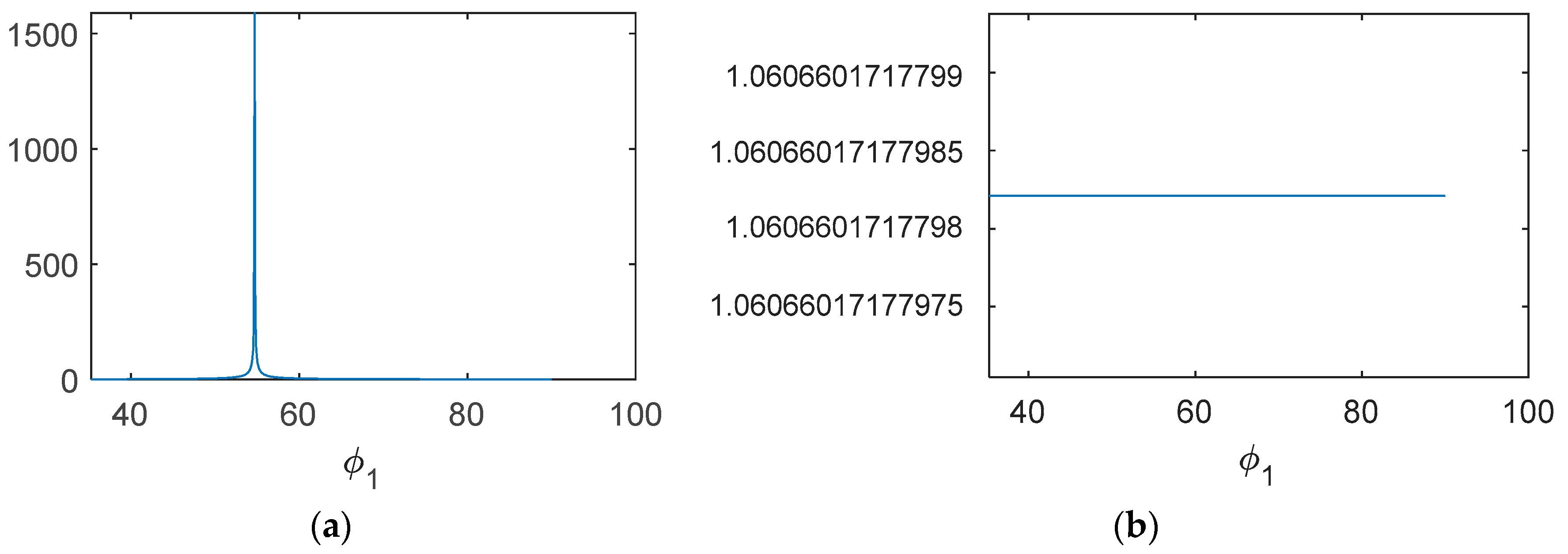
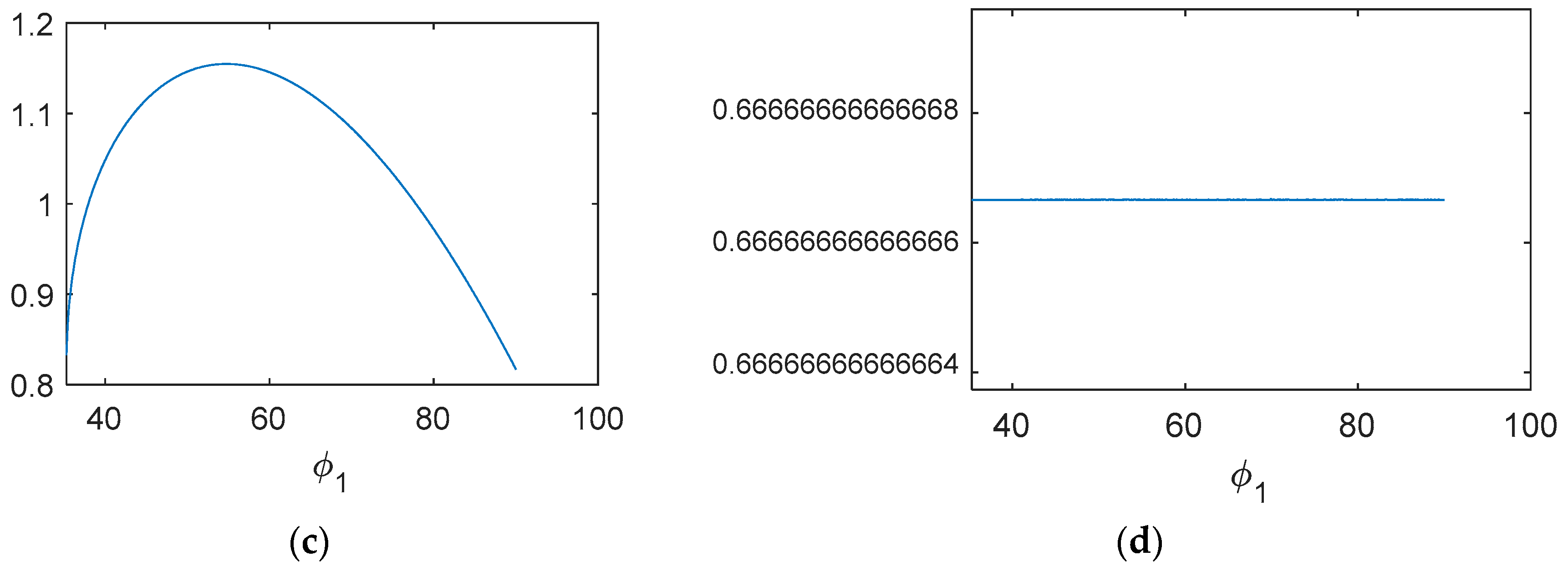
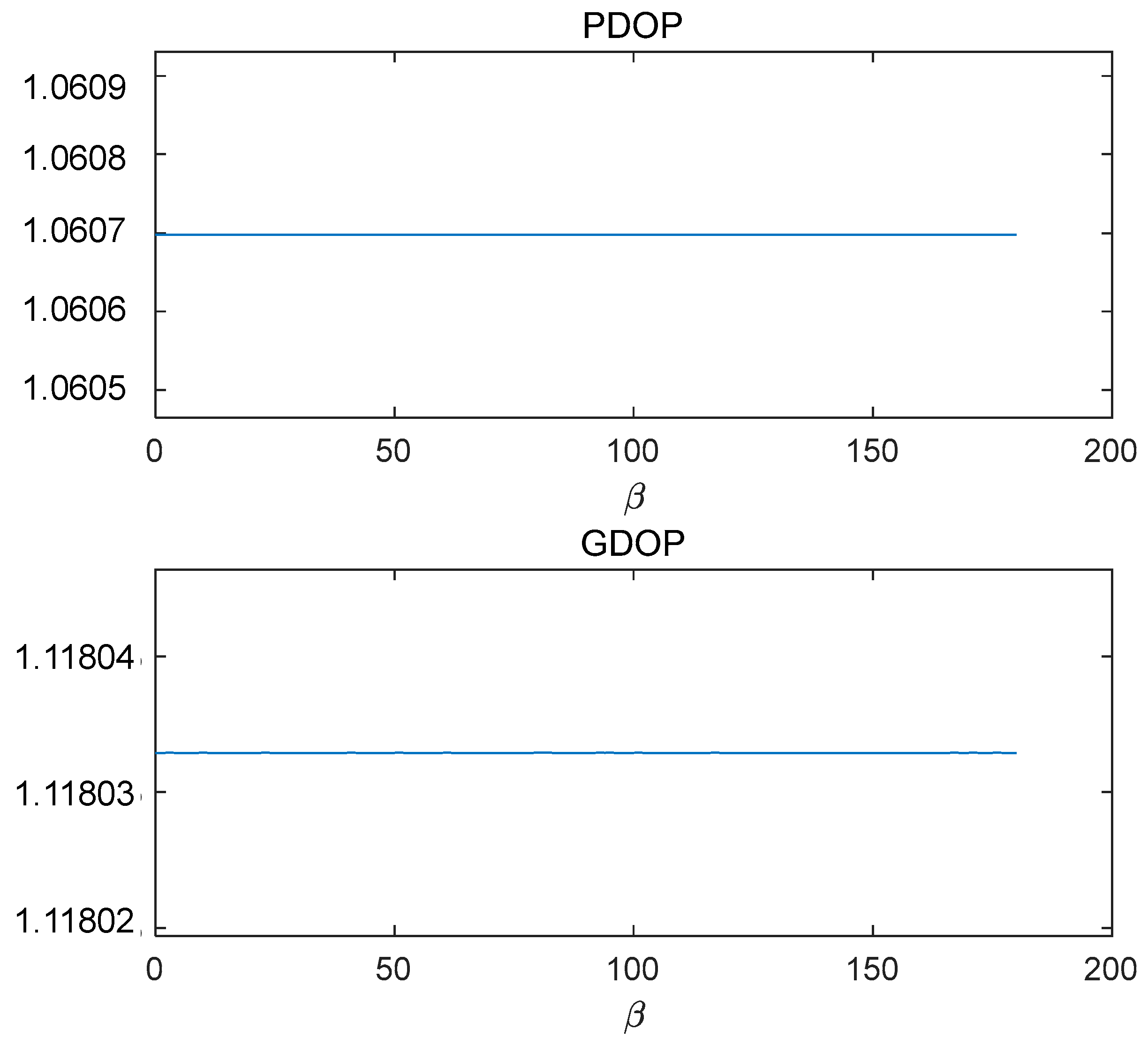
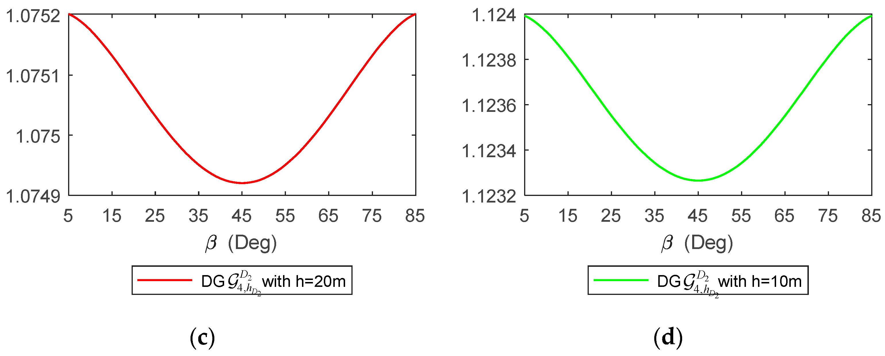
  • The trend of changes in Min_DOP, Center_DOP and E ( DOP g r o u n d ) with respect to the cone angle is consistent.
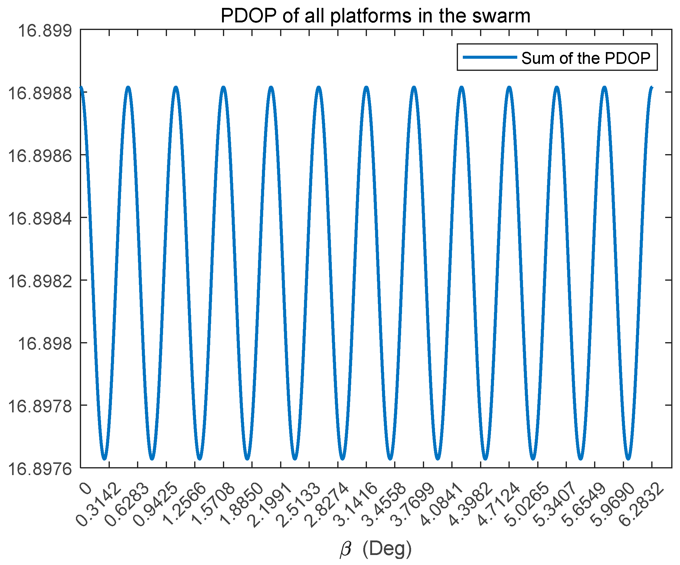
  • When the coning angles vary from 0 to π 2 , the variation amplitude of PDOP is much smaller than that of GDOP.
As mentioned, the average DOP value in the circular region centered on the ideal prior position of the target changes positively with the DOP at its center point. Therefore, the conditions for designing the optimal configuration for a single target are necessary conditions for obtaining the minimum average DOP on the target region. Now we have the optimal configuration to obtain minimum average DOP. The placements of all nodes in the DG are shown in Table 2 and in Figure 20.
In the optimal configuration designed, as shown in Figure 20, the minimum DOP at the target point would be obtained, but the average DOP would be affected by the height or radius of the cone configuration, as we mentioned in Figure 18. An extra group of parameters reflecting the size of the cone, which could influence the average DOP in the region, needs to be further researched. In fact, we have r i = h i tan φ i for each cone and tan φ i is a constant, i.e., r i and h i play the same role in reflecting the size of configuration.
The decrease in average DOP with the change in height is shown in Figure 21. In this set of simulations, we fixed the height of one DG and changed another. The result attributes that the enlargement for size of detection configuration benefits reducing the average of both GDOP and PDOP, which is consistent with the results shown in Figure 18. Specifically, when the radius of the configuration is smaller than the radius of the target region, the impact brought by radius changes on the average DOP is more significant. As the radius of the nested cone increases, the average DOP in the target region remains monotonically decreasing. Whereas the decrease in the average DOP will be very slow when the configuration reaches a huge size.
Above all, we draw conclusions about the parameter design for the nested cone configuration to obtain the average DOP in the target prior region. Because the trend of point DOP and the average DOP with coning angle is consistent, there is no need to change φ i and θ i for each cone when localization errors exist. The relative angle should maintain 45 ° to form the optimal configuration for the minimum of both point DOP and average DOP in the region. In addition, the larger configuration would theoretically lead to a lower average DOP, but the range between the detection node and the target should be considered with the sensors’ performance in practice.

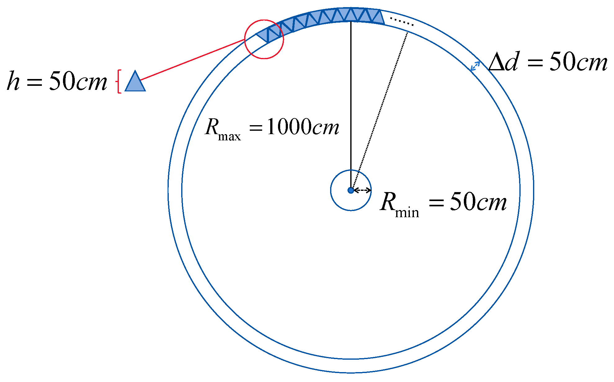
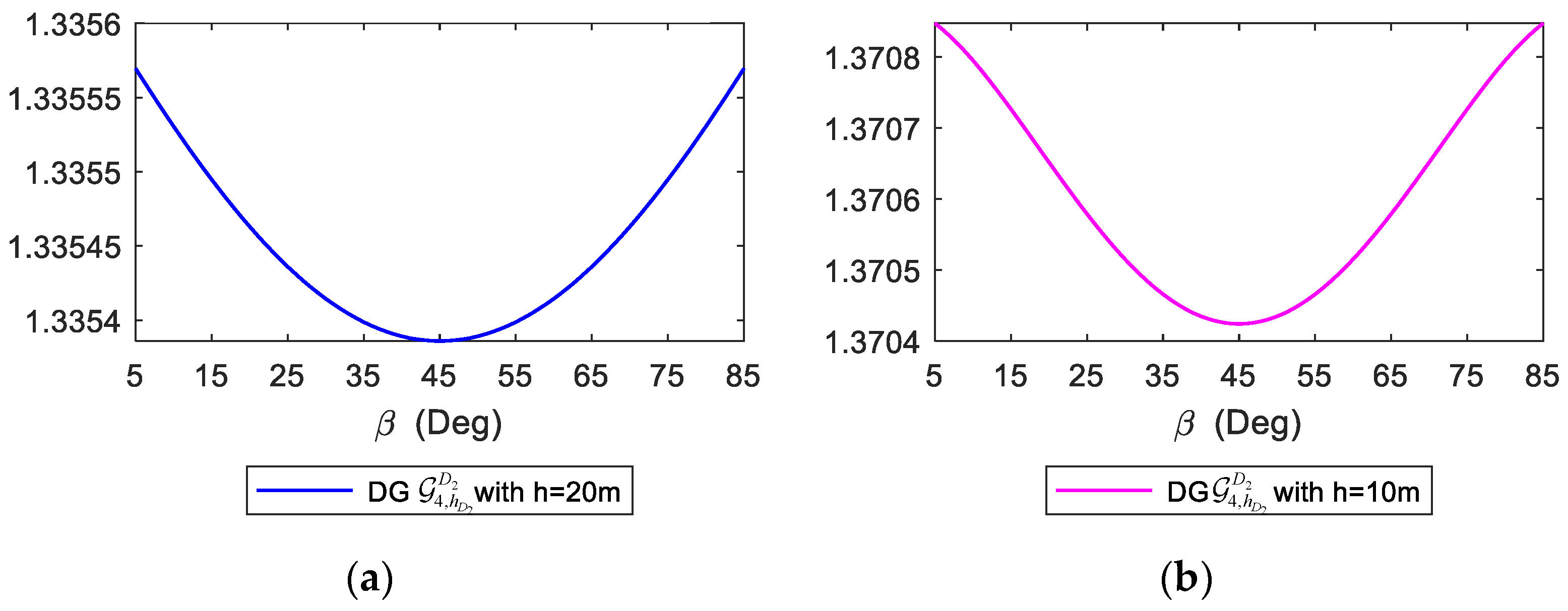
3.1.3. Design of Configuration for Minimum DOP with the Condition of Platforms’ Localization Error

In the research above, we create an optimal configuration for DGs to detect the ground target without considering the position error of platforms in the groups, which would invalidate the configuration and miss the minimum DOP. As shown in Figure 21, the unmanned platforms in DGs may not be exactly at their ideal position as arranged during the detection operation due to navigation errors. Considering the positioning error introduced by its own positioning performance, the true positions of each detection node will satisfy a Gaussian distribution centered on the ideal placed position.
If the drones leave their ideal arranged position, the accuracy of cooperative detection would directly decline. However, the position error cannot be eliminated or neglected in practice. To reduce the impact caught by position error, we carry out simulations to quantificationally analyze how DOP could increase with different position errors of platforms and study the relevant robustness of nest cone configurations.
In this section, we introduce the random positioning errors of each platform in the detection group, as shown in Figure 22. With the errors added, we applied Monte Carlo simulations 200 times repeatedly to calculate the point DOP and region DOP for each RMSE of the positioning error. The mathematical expectations and variances of the simulation with the same RMSE are shown in Figure 23.
In Figure 23, lines representing the expectation clearly show that both the prior position DOP and the average DOP on the target prior area will increase with the increase in positioning error of each detection node, which means the positioning error could deteriorate the detection accuracy severely. The sensitivity of GDOP to positioning errors is roughly the same as that of PDOP. When the positioning error reaches 5 m, E ( GDOP g r o u n d ) will increase by 9.5% and E ( PDOP g r o u n d ) will also increase by 8%. The GDOP distribution map of the target prior area is shown in Figure 24, with positioning RMSE = 1 m and RMSE = 3 m, respectively. As for the variances of 200 results of DOP with the same RMSE, the variance increases sharply with the increase in RMSE, which indicates that the detection accuracy is likely to be extremely poor or even divergent when the positioning accuracy of the detection platforms is low, which introduces great instability for the cooperative detection effect of the entire unmanned swarm.
In detail, at the beginning of the lines representing the average, the result with a small position disturbance is better than that without error. The reason can be explained in Figure 25 and Equation (29). In Figure 25a, influenced by small disturbances, the optimal configuration formed by the detection nodes is not severely disrupted but rather slightly increases in size. According to the result obtained in Section 3.1.2, the magnification of size would lead to a lower average DOP without considering the positioning error. Obviously, the conclusion also suits the situation that the RMSE of the detection nodes’ position is small. Another situation causing a lower average DOP is shown in Figure 25b. Without destroying the form of optimal configuration, the center of the projected circle deviates from the prior target point. In Equation (29), more DOP samples will be taken at the ring with a larger radius, which leads to the incorrect statistical average DOP.
The results reflect that the configuration with a small size would suffer severe influence from positioning errors. We enlarged one of the cones formed by G 4 , h D 2 D 2 with parameters φ 2 and θ 2 for optimal configuration. We designed and carried out simulations repeatedly, then plotted the result of the new configuration in Figure 26. Compared with Figure 24, incorrect statistical values disappear, and the DOP curves ascend quite slowly with the amplification of 2.1% for PDOP and 2.6% for GDOP when the RMSE is 5 m. In addition, the variances of DOP significantly decrease, indicating that the larger configuration would display stronger robustness against positioning errors of detection platforms.
The obvious conclusion obtained from the statistics of the Monte Carlo simulation prove the deterioration of DOP is mainly caused by destroying the configuration formed by DGs, reflecting the configuration designed based on Theorem 1, and Theorem 2 should be the optimal configuration to obtain minimum DOP, not only at the point but also covering the region. The result also shows clearly that the size of the detection configuration should be as large as possible within the measuring range for sensors to resist the influence caused by positioning errors, which is a vital scheme to ensure detection accuracy. Another way to deal with this problem is to improve the accuracy of localization of platforms in DGs, which is the main target for the design of AGs in the swarm.

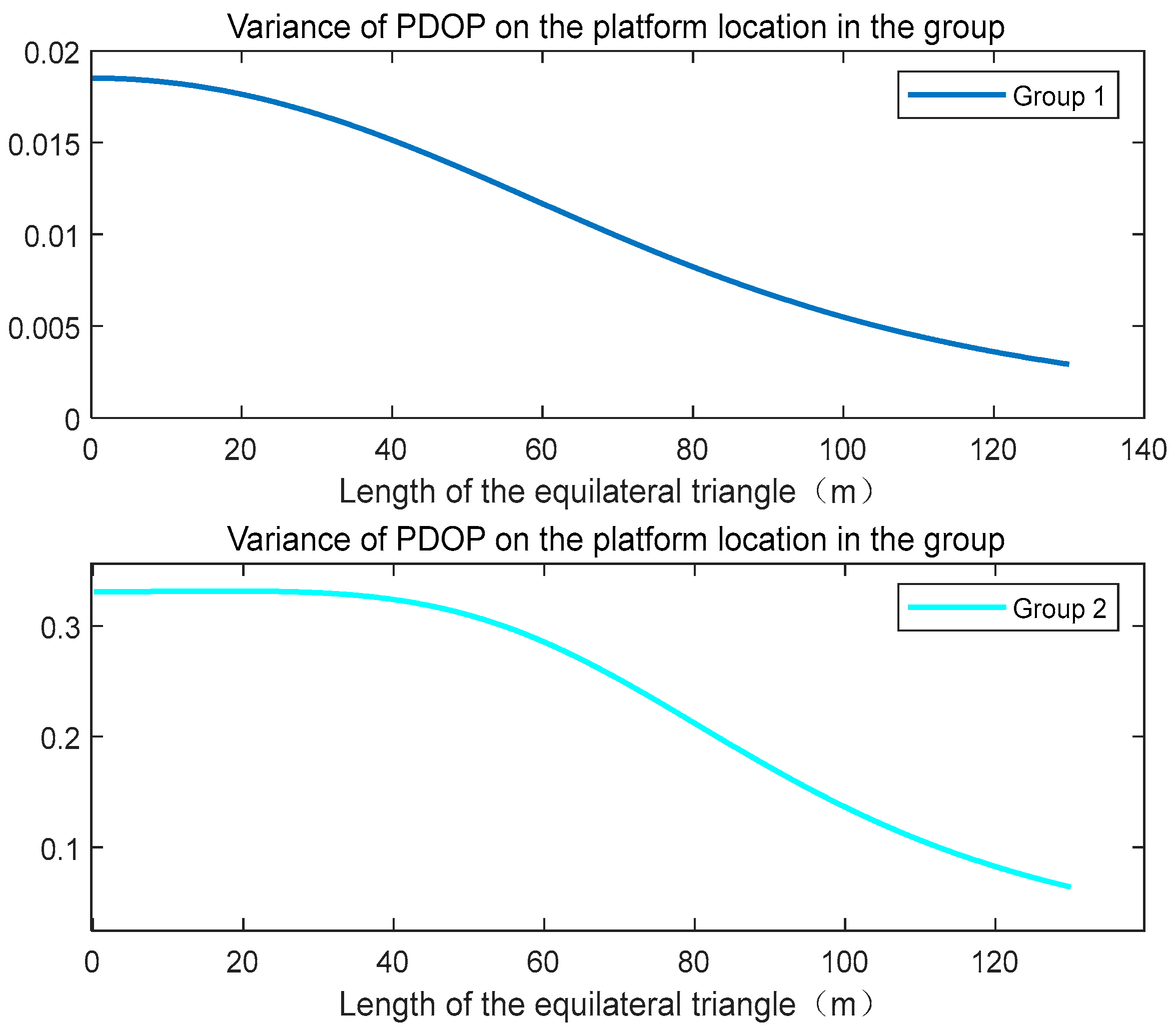
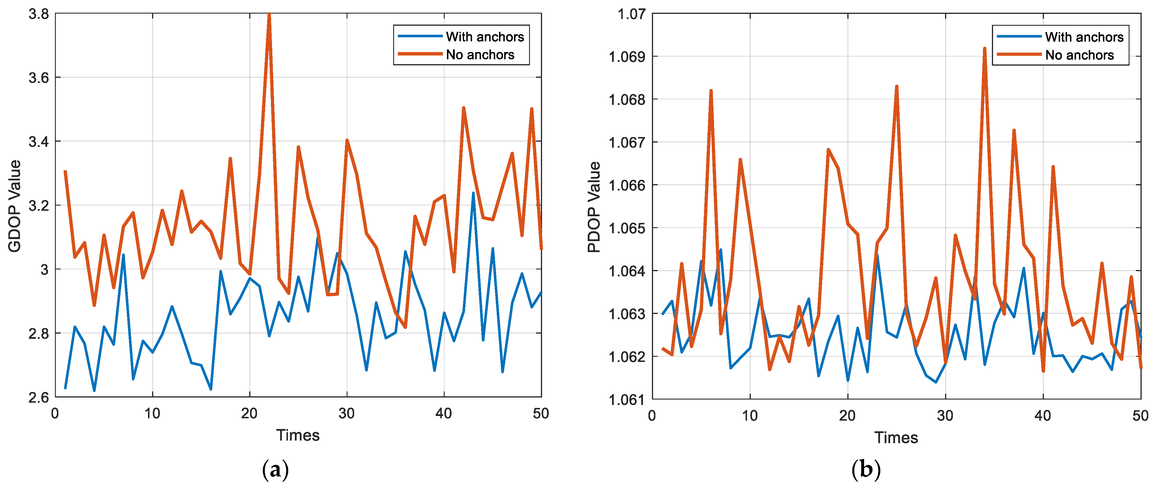
3.2. The Design of Configuration for AG

Because the size of the anchor configuration would be much larger compared with the anchors’ positioning errors, especially since all nodes G A , n i i are equipped with a high-accuracy navigation system, we ignore the stochastic error of nodes’ locations in the configuration design for AG. As mentioned above, the configuration design of AG is independent, serving to improve the positioning accuracy of nodes in DGs within the same swarm.
Two parameters should be determined in this step: The length of the equilateral triangular configuration and the relative angle β A between AG and DGs. In this section, we rechoose the parameters of nested cone configuration to be closer to reality: φ 1 = 45 ° and φ 2 = 65.91 ° . The heights of G 4 , h D 1 D 1 and G 4 , h D 2 D 2 are fixed as 30 m and 20 m, respectively. As set in Section 3.1, the GDOP cannot be calculated because the number of anchors is less than 4, so we only apply the sum of PDOP of 8 nodes in DG as the revenue function. The value of each PDOP at the detection node with increasing l is shown in Figure 27 and Figure 28.
In the figures, the PDOP at each placement for the detection node is not monotonically decreasing with the expansion of AG configuration. Two special positions must be noted: One is the inflection point marked as x i g . When l i = x i g , the sum of PDOP within one DG would reach its minimum. We mark another point worth focusing on as x i k , which satisfies d D O P i ( l ) d l l = x i k = 1 . When l i < x i k , the curve of PDOP is sharply decreased, whereas when l i > x i k , the decline with increasing l is slow.
By comparing Figure 27 and Figure 28, it can be concluded that x i k is related to the coning angle φ and radius r of the cone configuration of the DG. If the radius of the coning angle becomes larger, the value of x i k will be higher. Similarly, x i g would also be affected by the 2 parameters mentioned, and the larger the radius is, the bigger x i g will be as well. The difference is that the influence of the change in coning angle is contrary, i.e., we will obtain a smaller x i g in a cone with a larger φ . In Figure 29, we plot x i k and x i g with different parameters on one number axis to visually present the conclusion.
Furthermore, by zooming in parts of the curves in Figure 27 and Figure 28, the PDOP of different nodes in one group varies more slightly with l i becoming longer, which is demonstrated by the variance statistics in Figure 30. Although the variance is not vital for the accuracy of the localization for detection nodes, maintaining consistent positioning accuracy for all nodes within one group would benefit the control of drones in practice and better suit the assumption of homogeneous DG we set.
Similar to the design of the detection configuration, in addition to determining the size of the anchor configuration, it is also necessary to determine the relative angle β , which is shown in Figure 31. The determination of relative angle can refer to the conclusion in Section 3.1.2, which is related to the properties of rotationally symmetric images.
Applying the design of detection configuration in Section 3.1, we note that the detection configuration and anchor configuration are both central symmetry figures. The new figure combined by 2 configurations would coincide with the β rotating per π 6 . Define β = 0 when the triangle’s median coincides with the square’s diagonal. Setting equal positioning weights for all detection nodes, we obtain the objective function as Equation (30). The value of this function with the rotation of β is shown in Figure 32.
max ( DOP n o d e ) = max ( j = 1 q ( α j i = 1 n i DOP n o d e _ i ) ) α j = 1 q ,   j = 1 ,   2 q
The curve in Figure 32 reflects that the sum of PDOP varies periodically with a period as π 6 , which is consistent with the geometric characteristics of the swarm configuration. The objective function would reach its minimum when β = π 4 + k π 6 ,   k = 0 ,   1 ,   2 , ,   11 .
We noticed that the objective function includes DOPs of all nodes in 2 DGs with different configurations. In fact, for a single DG, the condition for obtaining the minimum sum of DOPs is the same as the conclusion mentioned. When the axis of the regular triangle coincides with the diagonal of the square, the minimum sum of DOPs at all detection nodes within the group is obtained. As shown in Figure 33 and Figure 34, the minimum sum of DOPs for DG1 and DG2 would be obtained when β = π 4 + k π 6 ,   k = 0 ,   1 ,   2 , ,   11 and β = k π 6 ,   k = 0 ,   1 ,   2 , ,   11 , respectively.
Comparing Figure 32 with Figure 33 and Figure 34, it is not difficult to find that the change trend of the objection function is quasi-synchronous with the sum of PDOPs of nodes in DG2 due to the greater amplitude of the change in the sum value of DG2 than that of DG1. This phenomenon indicates that if β is not the optimal value as designed, the sum PDOP of the group would be more influenced.
In conclusion, we find the best relative angle β to make the AG localize all nodes in DGs with the best accuracy. The best l for optimal configuration can also be found according to the curves. In fact, PDOPs vary extremely sightly when the l is bigger than x i k or close to x i g , which provides minor influence on the accuracy of the localization to detection nodes. For this reason, we trust any l i ( x i k , x i g ) would be a decent parameter if l = x i g is hard to realize for ground vehicles when facing complex environments.

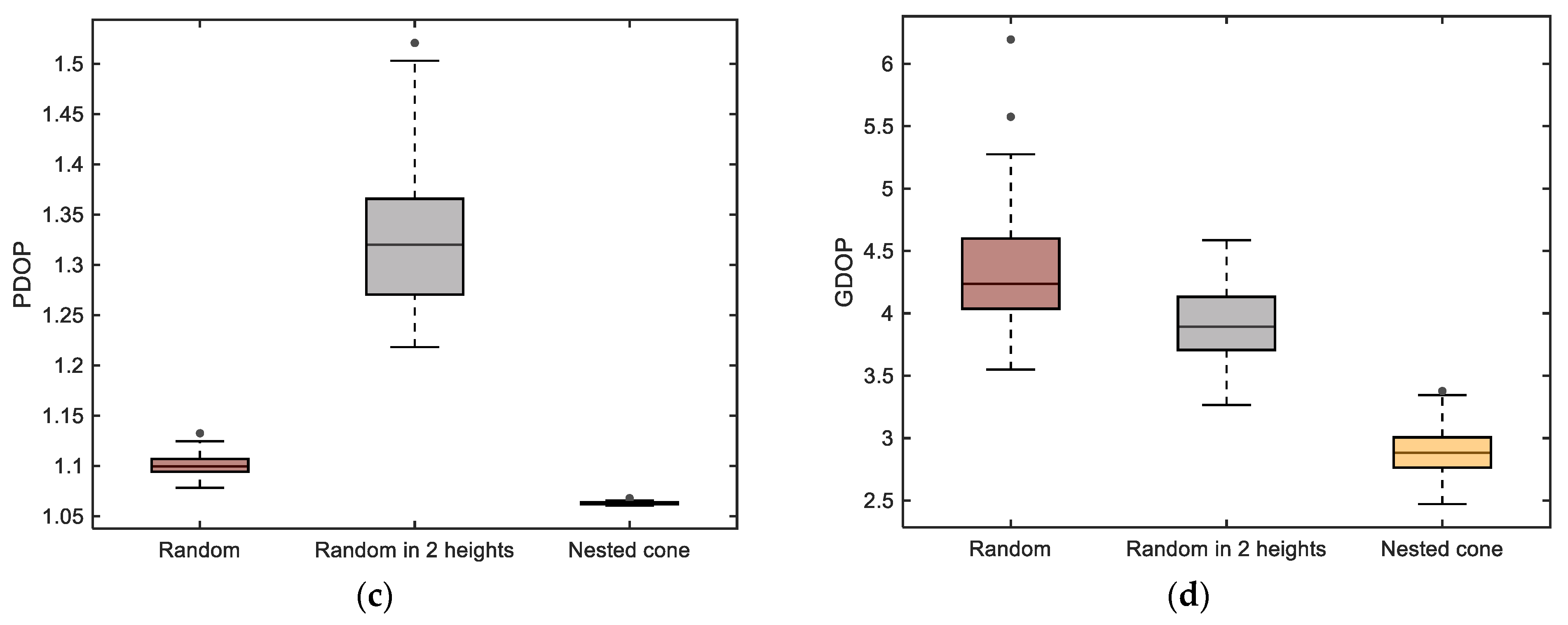
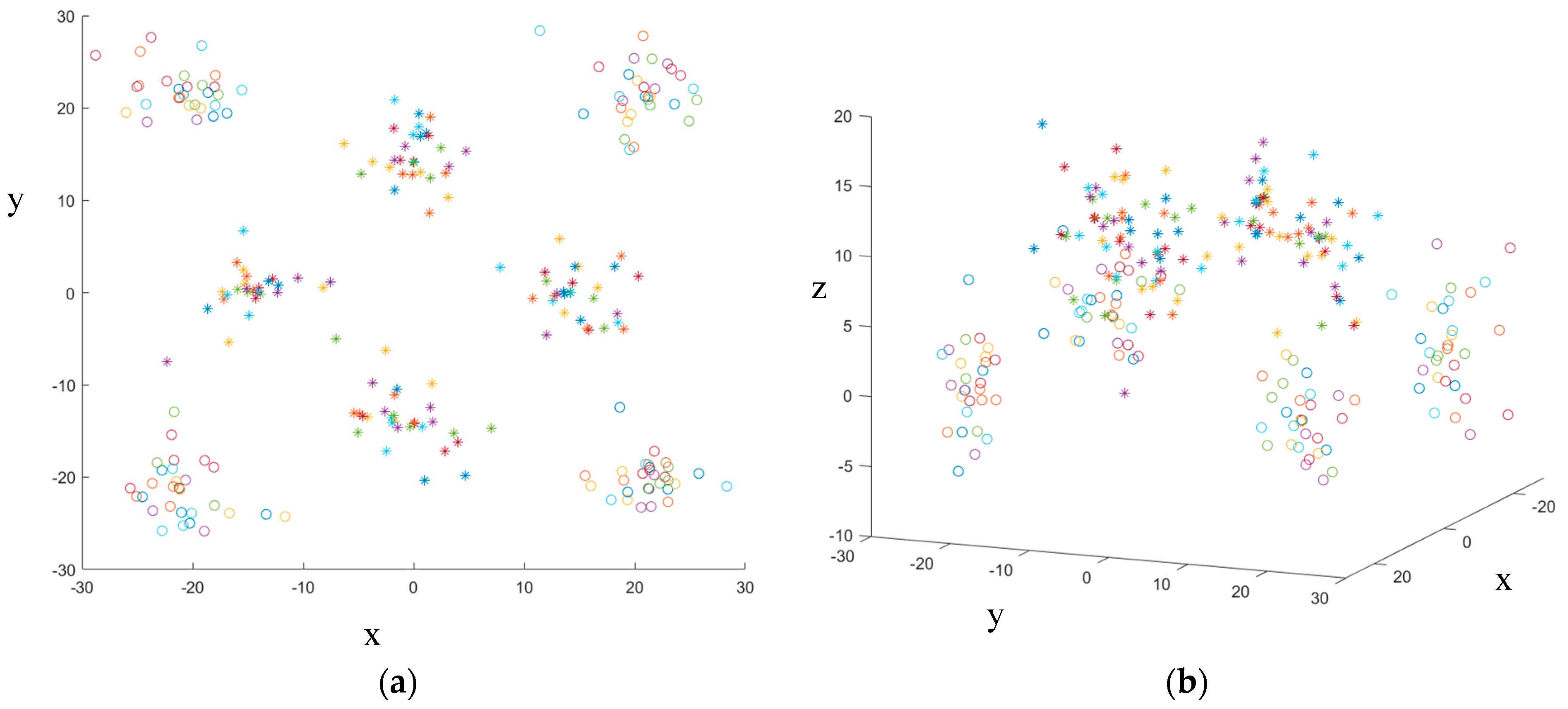
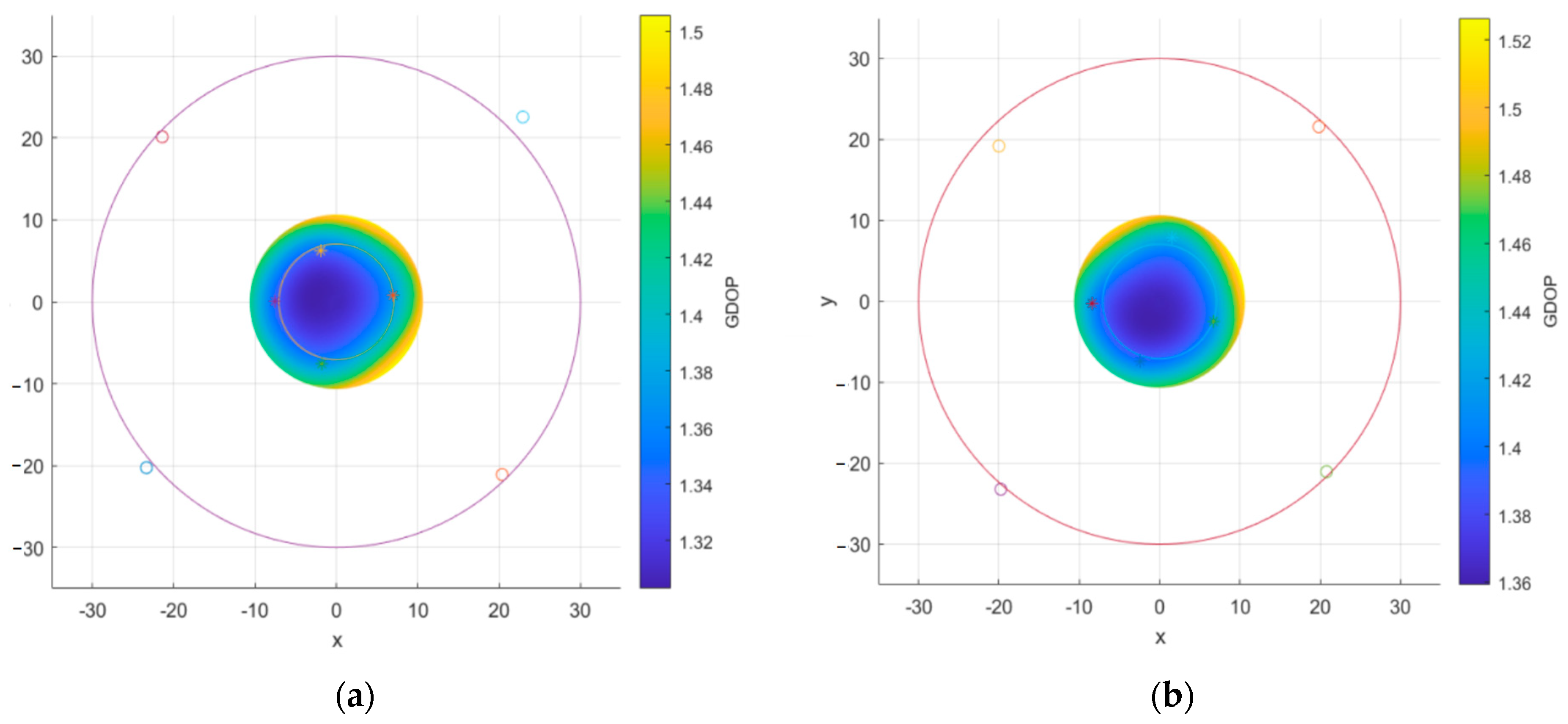
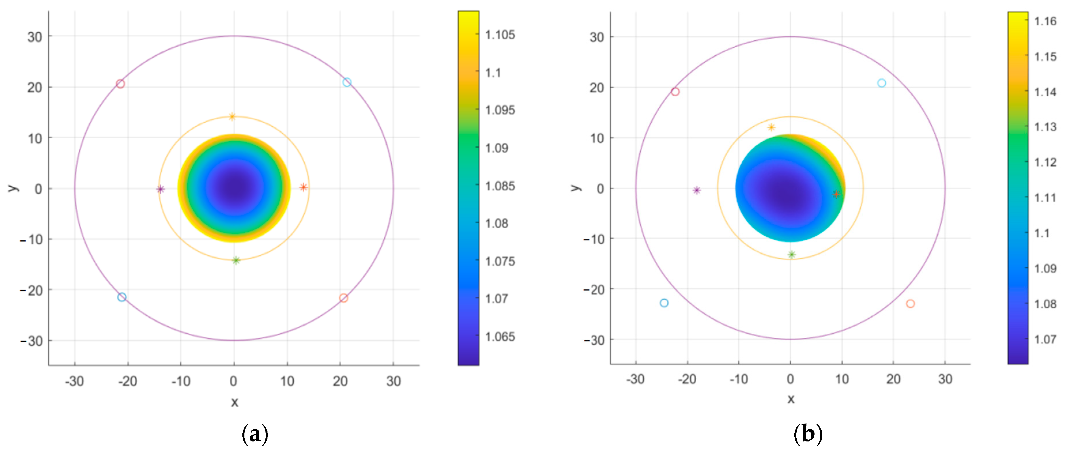
3.3. Comparison between Designed Optimal Configuration and Random Placement

In this subsection, we calculate the PDOP of one set of swarms equipped with different sensors for detection. In the simulation, the RMSE of localization of nodes in DGs is set at 3 m without cooperative navigation, and the range error of nodes in AG is 1 m. We selected the results obtained by our method and random placement to carry out the comparative experiment, in which we considered the positioning error of detection UAVs and conducted 100 Monte Carlo simulations. By comparing their DOP at the target point, we determine the performances of different configurations.
The swarm consists of 6 UAVs and 3 UGVs. The placement of six nodes based on the different methods is presented in Table 3. As the design based on the method proposed in this paper, we divide 6 UAVs into 2 groups at different heights. As comparisons, one random configuration places detection nodes in 2 heights as well, and another just places all nodes in one height. In Figure 35, we show the average DOP on the circular region with a radius of 5 m on the ground. From the result, we can see both GDOP and PDOP meet a lower value, which means the relevant configuration could lead to better detection accuracy. The boxplots show the statistical data of all simulations, which we could use to analyze the robustness of different configurations for DOP. Obviously, the nested cone configuration performs better. However, when facing positioning errors, the GDOP would be affected much more than the PDOP.
As for the fixed optimal configurations for DGs, we compare the average DOP after adding AG with optimal placement and without AG in Figure 36. By adding UGVs as anchors, the average PDOP and GDOP on the prior region decreased by 9.1% and 1.1%, respectively. In fact, the AG would perform a more vital role when the localization errors of detection nodes rise up by more than 3 m, as we have set now.

4. Conclusions

This article proposes a design method for the optimal detection configuration of a heterogeneous swarm based on the nested cone configuration. Considering positioning errors at detection nodes and the prior information of the target, we conduct a large number of simulation experiments to determine the parameters for the configuration of a swarm to obtain the minimum DOP. Besides the optimal conditions, the threshold for the design of configuration parameters was also discussed and given as recommendations. This is because, in complex engineering practice, the placement of nodes is often interfered with by more factors, such as the performance of unmanned platforms and airborne sensors, mission requirements, including obstacle limitations, terrain factors, and mission requirements. Therefore, we strive to provide an informative suggestion through the experiments in the paper in order to make appropriate adjustments to the theoretical optimal configuration based on the specific situations in practical applications.
Oriented to the heterogeneous swarm, the design of an optimal detection configuration based on the nested cone has the following advantages:
  • The process of grouping is more intuitive, suiting the working characteristics of heterogeneous swarms much better.
  • The modeling of different groups distributed in different cones is independent of each other, making it easy to add constraints to specific groups based on specific tasks or establish conditional functions when facing more complex optimization problems.
  • The calculation of DOP is simple and fast, which improves the speed of optimal design.
In summary, the design method in this article not only leverages the advantages of heterogeneous swarms but also has a fast optimization speed and good applicability. However, some questions remain unsettled:
  • The calculation of DOP requires the noise of airborne sensors to be independent white noise, but the noise characteristics of sensors such as LiDAR and airborne radar do not strictly satisfy this requirement.
  • The design of the nested cone configuration relies on prior position information about the target.
  • The design of this formation only focuses on the optimal DOP, which is the detection accuracy requirement, without considering detection coverage, efficiency, and other indicators.
In addition, the article utilizes sufficient experimental evidence to prove that the new configuration remains optimal after superposing different groups with optimal configurations. There is indeed a lack of strict mathematical proof in the design of certain parameters, which is also a major challenge for nested cone models in transitioning from the optimal design for a single point to the optimal design for a region.
When it comes to piratical engineering, the designed method based on nested cones has an advantage in convergent speed and stability compared with other methods facing convex optimization problems. Different from the sensor placement, the arrangement of all nodes relies on the instant communication system because the nodes are all movable, which requires more research to avoid or reduce the effect brought by communication latency.
Overall, the cone nested configuration for minimum DOP is a suitable design solution for heterogeneous swarm detection. In future work, proving the problem using strict mathematical proof would be a major focus. In addition, combining other optimization algorithm ideas or flexibly combining deep neural networks to design the parameters of the formation will make the nested cone formation more widely applicable and achieve better design effects.

Author Contributions

Conceptualization, Y.L.; methodology, Y.L.; software, Y.L.; validation, Y.L. and R.Y.; formal analysis, P.J.; investigation, Y.G.; resources, Z.X.; data curation, Y.G.; writing—original draft preparation, Y.L. and Y.M.; writing—review and editing, Y.L. and Y.M.; supervision, Y.G.; project administration, Y.L. and R.Y.; funding acquisition, R.Y. and P.J. All authors have read and agreed to the published version of the manuscript.

Funding

The APC was funded by Natural Science Foundation of China: 62203456, 42276199.

Data Availability Statement

The data presented in this study are available on request from the corresponding author. The data are not publicly available due to the further research relying on the data is still underway.

Acknowledgments

Thanks to the help and hardware support from Yalin Fei and teachers in the Navigation and Guidance Laboratory.

Conflicts of Interest

The authors declare no conflicts of interest.

References

  1. Yang, A.W.; Liang, X.L.; Hou, Y.Q. An Autonomous Cooperative Interception Method with Angle Constraints Using a Swarm of UAVs. IEEE Trans. Veh. Technol. 2023, 72, 15436–15449. [Google Scholar] [CrossRef]
  2. Cai, W.Y.; Liu, Z.Q.; Zhang, M.Y. Cooperative Artificial Intelligence for underwater robotic swarm. Robot. Auton. Syst. 2023, 164, 104410. [Google Scholar] [CrossRef]
  3. Farid, A.M.; Kuan, L.M. Effective UAV patrolling for swarm of intruders with heterogeneous behavior. Robotica 2023, 41, 1673–1688. [Google Scholar] [CrossRef]
  4. Chen, K.; Fan, C.L. Heterogeneous swarm control based on two-layer topology. Int. J. Robust Nonlinear Control 2023, 33, 1. [Google Scholar] [CrossRef]
  5. Zhen, Z.Y.; Wen, L.D. Improved contract network protocol algorithm based cooperative target allocation of heterogeneous UAV swarm. Aerosp. Sci. Technol. 2021, 119, 107054. [Google Scholar] [CrossRef]
  6. Jiang, T.H. Research on Formation Deployment and Effectiveness Evaluation Method for Multi-UUV Cooperative Operations. Master’s Thesis, Control Science and Engineering Harbin Engineering University, Harbin, China, 2020. [Google Scholar]
  7. Chen, G.J. Research on the Construction and Optimization of Multi-UUV Formations for Collaborative Detection. Master’s Thesis, Control Science and Engineering Harbin Engineering University, Harbin, China, 2021. [Google Scholar]
  8. Xu, S.; Wu, L.L. A Hybrid Approach to Optimal TOA-Sensor Placement With Fixed Shared Sensors for Simultaneous Multi-Target Localization. IEEE Trans. Signal Process. 2022, 70, 1197–1212. [Google Scholar] [CrossRef]
  9. Xu, S.; Rice, M. Optimal TOA-sensor placement for two target localization simultaneously using shared sensors. IEEE Commun. Lett. 2021, 25, 2584–2588. [Google Scholar] [CrossRef]
  10. Xu, S. Optimal Sensor Placement for Target Localization Using Hybrid RSS, AOA and TOA Measurements. IEEE Commun. Lett. 2020, 24, 1966–1970. [Google Scholar] [CrossRef]
  11. Chen, S.J.; Ho, K.C. Achieving Asymptotic Efficient Performance for Squared Range and Squared Range Difference Localizations. IEEE Trans. Signal Process. 2013, 61, 2836–2849. [Google Scholar] [CrossRef]
  12. Beck, A.; Stoica, P.; Li, J. Exact and approximate solutions of source localization problems. IEEE Trans. Signal Process. 2008, 56, 1770–1778. [Google Scholar] [CrossRef]
  13. Zhou, R.H.; Sun, H.M.; Li, H. TDOA and track optimization of UAV swarm based on D-optimality. J. Syst. Eng. Electron. 2020, 31, 1140–1151. [Google Scholar] [CrossRef]
  14. Zhou, R.H.; Sun, H.M.; Li, H. Hybrid TDOA/FDOA and track optimization of UAV swarm based on A-optimality. J. Syst. Eng. Electron. 2023, 34, 149–159. [Google Scholar] [CrossRef]
  15. Zhang, F.B.; Wu, X.Q.; Ma, P. Consistent Extended Kalman Filter-Based Cooperative Localization of Multiple Autonomous Underwater Vehicles. Sensors 2022, 22, 4563. [Google Scholar] [CrossRef] [PubMed]
  16. Fang, X.P.; Li, J.B. Optimal AOA Sensor-Source Geometry with Deployment Region Constraints. IEEE Commun. Lett. 2022, 26, 793–797. [Google Scholar] [CrossRef]
  17. Xu, B.; Fei, Y.L.; Wang, X.Y. Optimal topology design of multi-target AUVs for 3D cooperative localization formation based on angle of arrival measurement. Ocean Eng. 2023, 271, 113758. [Google Scholar] [CrossRef]
  18. Wang, Y.; Zhou, T.; Yi, W. A GDOP-Based Performance Description of TOA Localization with Uncertain Measurements. Remote Sens. 2022, 14, 910. [Google Scholar] [CrossRef]
  19. Ganesh, L.; Rao, G.S. TDOA Measurement Based GDOP Analysis for Radio Source Localization. Procedia Comput. Sci. 2016, 85, 740–747. [Google Scholar] [CrossRef]
  20. Sharp, I.; Yu, K.; Guo, Y.J. GDOP Analysis for Positioning System Design. IEEE Trans. Veh. Technol. 2009, 58, 3371–3382. [Google Scholar] [CrossRef]
  21. Xue, S.Q.; Yang, Y.X. Understanding GDOP minimization in GNSS positioning: Infinite solutions, finite solutions and no solution. Adv. Space Res. 2017, 59, 775–785. [Google Scholar] [CrossRef]
  22. Zhang, J.; Wu, Z.L. PDOP Analysis of Walker Constellation. Astron. Res. Technol. 2009, 2, 107–118. [Google Scholar]
  23. Xue, S.Q.; Yang, Y.X. A Nested Cone Structure for Minimum GDOP Positioning Configuration. Geomat. Inf. Sci. Wuhan Univ. 2014, 11, 1369–1374. [Google Scholar]
  24. Xue, S.Q.; Yang, Y.X. The minimum GDOP positioning configuration solution set derived from orthogonal trigonometric functions. Geomat. Inf. Sci. Wuhan Univ. 2014, 7, 820–825. [Google Scholar]
  25. Wang, C.Y. Study on UWB Positioning Method and Configuration Optimization. Doctor’s Thesis, China University of Mining and Technology, Xuzhou, China, 2020. [Google Scholar]
  26. Ding, L.Q.; Liu, Y.F.; Wu, N. Research on Unmanned Aircraft Collaborative Detection Configuration. Command Control Simul. 2022, 44, 12–18. [Google Scholar]
  27. Miao, S.; Hou, J.Y. Dynamic base stations selection method for passive location based on GDOP. PLoS ONE 2022, 17, e0272487. [Google Scholar] [CrossRef] [PubMed]
  28. Wan, J.; Dang, Y.M. Research of Buoy Array with Minimum GDOP for Underwater Positioning. Bull. Surv. Mapp. 2016, 5, 22–25, 31. [Google Scholar]
  29. Liu, Y.L.; Yu, R.H. Attitude Determination for Unmanned Cooperative Navigation Swarm Based on Multivectors in Covisibility Graph. Drones 2023, 7, 40. [Google Scholar] [CrossRef]
  30. Zhu, X.D.; Lai, J.Z. Robust adaptive cooperative localization method for multiple UAVs based on configuration optimization. J. Chin. Inert. Technol. 2023, 31, 650–658. [Google Scholar]
  31. Wang, C.Y.; Ning, Y.P. Optimized deployment of anchors based on GDOP minimization for ultra-wideband positioning. J. Spat. Sci. 2022, 67, 455–472. [Google Scholar] [CrossRef]
  32. Zhao, J.; Sun, J.M. Distributed coordinated control scheme of UAV swarm based on heterogeneous role. Chin. J. Aeronaut. 2022, 35, 81–97. [Google Scholar] [CrossRef]
  33. Xue, S.Q.; Yang, Y.X. Positioning configurations with the lowest GDOP and their classification. J. Geod. 2015, 89, 49–71. [Google Scholar] [CrossRef]
Figure 1. e i in the 3D Cartesian coordinate system.
Drones 08 00011 g001
Figure 2. The relationship between the lowest DOP and the number of platforms.
Drones 08 00011 g002
Figure 3. The configuration geometry with the lowest GDOP. (a) Cone configuration. (b) Descartes configuration. (c) Walker configuration.
Drones 08 00011 g003
Figure 4. The two-dimensional cone configuration. The stars represent the node and the triangle represents the target.
Drones 08 00011 g004
Figure 5. Three-dimensional cones: (a) single cone configuration; (b) coaxial nested cone configuration.
Drones 08 00011 g005
Figure 6. Three-dimensional cone configuration and its orthogonal projection configuration. The stars represent the node and the triangle represents the target.
Drones 08 00011 g006
Figure 7. Three types of platforms in the swarm: (a) UGV; (b) small drones; (c) large drones.
Drones 08 00011 g007
Figure 8. Platforms divided into different groups for cooperative detection.
Drones 08 00011 g008
Figure 9. Optimal configuration design method for cooperative heterogeneous unmanned swarm.
Drones 08 00011 g009
Figure 10. The design for G D , n j j and G A , n i i .
Drones 08 00011 g010
Figure 11. Detection configuration for drones: (a) single cone detection configuration G 4 , 3 ; (b) nested cone configuration G 4 , 3 1 + G 4 , 3 2 .
Drones 08 00011 g011
Figure 12. The 2D configuration G 4 , 2 with the minimum GDOP.
Drones 08 00011 g012
Figure 13. The relationship between variables and φ i (a) GDOP (b) PDOP (c) cos ( ϕ 1 ) + cos ( ϕ 2 ) (d) cos 2 ( ϕ 1 ) + cos 2 ( ϕ 2 ) .
Drones 08 00011 g013aDrones 08 00011 g013b
Figure 14. The orthogonal projection of the placement of G 4 , h D 1 D 1 and G 4 , h D 2 D 2 .
Drones 08 00011 g014
Figure 15. GDOP and PDOP remain constant with the change in relative angle β .
Drones 08 00011 g015
Figure 16. The inaccurate prior information causes the tip of the cone to not be at the target exactly.
Drones 08 00011 g016
Figure 17. The distribution map of the DOP value: (a) β = 0 (b) β = 45 ° (c) β = 60 ° .
Drones 08 00011 g017
Figure 18. Differentiation method of the prior target region.
Drones 08 00011 g018
Figure 19. Variation of DOP in the prior target region near the cone tip with the relative angle β . (a,b) Average GDOP on the target region. (c,d) Average PDOP on the target region.
Drones 08 00011 g019aDrones 08 00011 g019b
Figure 20. The distribution map of the DOP value in the target prior region with optimal configuration for DGs. The symbol “*” represents the nodes in G 4 , h D 1 D 1 and circles represent the nodes in G 4 , h D 2 D 2 . (a,b) GDOP distribution map. (c,d) PDOP distribution map.
Drones 08 00011 g020
Figure 21. Drones may leave their ideal arranged position due to navigation errors.
Drones 08 00011 g021
Figure 22. Location of detection nodes under random position errors in the experiments.The symbol “*” represents the nodes in G 4 , h D 1 D 1 and circles represent the nodes in G 4 , h D 2 D 2 . (a) Projection distribution on x-y plane. (b) 3D spatial distribution.
Drones 08 00011 g022
Figure 23. Expectations and variances of DOP at the target point the target prior area with height of G 4 , h D 2 D 2 being 10 m: (a) Average value of GDOP in simulations. (b) Average value of PDOP in simulations. (c) Variance of GDOP in simulations. (d) Variance of PDOP in simulations.
Drones 08 00011 g023aDrones 08 00011 g023b
Figure 24. The GDOP distribution map of the target prior area. (a) RMSE = 1 m (b) RMSE = 3 m.
Drones 08 00011 g024
Figure 25. Special cases for lower DOP caused by positioning error. (a) Radius increases without destroying the cone. (b) The ideal cone shifts without being destroyed.
Drones 08 00011 g025
Figure 26. Expectations and variances of DOP at the target point the target prior area with a height of 20 m: (a) Average value of GDOP in simulations. (b) The average value of PDOP in simulations. (c) Variance of GDOP in simulations. (d) Variance of PDOP in simulations.
Drones 08 00011 g026aDrones 08 00011 g026b
Figure 27. PDOP on the platforms’ placement in DG 1.
Drones 08 00011 g027
Figure 28. PDOP on the platforms’ placement in DG 2.
Drones 08 00011 g028
Figure 29. The position of x i k and x i g in different cones on the number axis.
Drones 08 00011 g029
Figure 30. Variance of PDOP on the location of platforms in the group.
Drones 08 00011 g030
Figure 31. The relationship between the AG and DGs.
Drones 08 00011 g031
Figure 32. The sum of PDOP at all platforms’ placements in the swarm.
Drones 08 00011 g032
Figure 33. Sum of PDOP on the placements of platforms in the DG 1.
Drones 08 00011 g033
Figure 34. Sum of PDOP on the placements of platforms in the DG 2.
Drones 08 00011 g034
Figure 35. Results of simulation for different configurations: (a,c) PDOP in each simulation. (b,d) GDOP in each simulation.
Drones 08 00011 g035aDrones 08 00011 g035b
Figure 36. Effect of AG on DOP on prior region: (a) GDOP. (b) PDOP.
Drones 08 00011 g036
Table 1. DOP at target point and the average DOP on the target prior region with different angle for nested cone configuration.
φ 1 = 35.26 ° φ 2 = 90 ° φ 1 = 37.08 ° φ 2 = 79.99 ° φ 1 = 45 ° φ 2 = 65.91 ° φ 1 = 53.76 ° φ 2 = 55.54 ° φ 1 = 40 ° φ 2 = 65 ° φ 1 = 50 ° φ 2 = 65 °
Min_GDOP1.321.572.6814.432.483.38
Min_PDOP1.061.061.061.061.071.06
Center_GDOP1.321.572.8732.252.583.75
Center_PDOP1.061.061.061.061.071.06
E ( GDOP g r o u n d ) 1.341.572.8024.062.553.63
E ( PDOP g r o u n d ) 1.061.071.071.081.071.07
Min_DOP represents the minimum value in the region. Center_DOP is the DOP at the target prior point. E ( DOP g r o u n d ) is the average DOP in the region.
Table 2. Locations of all nodes in the DG when forming the optimal configuration for minimum DOP.
DG   1   G 4 , h D 1 D 1 DG   2   G 4 , h D 2 D 2
Node 1 ( h 1 tan φ 1 cos θ 1 , 1 h 1 tan φ 1 sin θ 1 , 1 h 1 ) ( h 2 tan φ 2 cos θ 2 , 1 h 2 tan φ 2 sin θ 2 , 1 h 2 )
Node 2 ( h 1 tan φ 1 cos θ 1 , 2 h 1 tan φ 1 sin θ 1 , 2 h 1 ) ( h 2 tan φ 2 cos θ 2 , 2 h 2 tan φ 2 sin θ 2 , 2 h 2 )
Node 3 ( h 1 tan φ 1 cos θ 1 , 3 h 1 tan φ 1 sin θ 1 , 3 h 1 ) ( h 2 tan φ 2 cos θ 2 , 3 h 2 tan φ 2 sin θ 2 , 3 h 2 )
Node 4 ( h 1 tan φ 1 cos θ 1 , 4 h 1 tan φ 1 sin θ 1 , 4 h 1 ) ( h 2 tan φ 2 cos θ 2 , 4 h 2 tan φ 2 sin θ 2 , 4 h 2 )
θ 1 , 1 ,   θ 1 , 2 ,   θ 1 , 3 ,   θ 1 , 4 and θ 2 , 1 ,   θ 2 , 2 ,   θ 2 , 3 ,   θ 2 , 4 form an equal difference sequence separately with difference as 90 ° .
Table 3. Placements of nodes in DG in the swarm.
Detection
Nodes
Random FormationRandom Formation
in 2 Heights
Nested Method
x/my/mz/mx/my/mz/mx/my/mz/m
UAV15−3130−10−28031.6331.6320
UAV242353022150−31.6331.6320
UAV3−621330−2−50−31.63−31.6320
UAV4−555430−725031.63−31.6320
UAV512−27302711030.00030
UAV615−3230−12−2160030.0030
UAV7321530152160−30.00030
UAV8−122730−21−1600−30.0030
Disclaimer/Publisher’s Note: The statements, opinions and data contained in all publications are solely those of the individual author(s) and contributor(s) and not of MDPI and/or the editor(s). MDPI and/or the editor(s) disclaim responsibility for any injury to people or property resulting from any ideas, methods, instructions or products referred to in the content.

