Observing Individuals and Behavior of Hainan Gibbons (Nomascus hainanus) Using Drone Infrared and Visible Image Fusion Technology

Abstract

The Hainan gibbon (Nomascus hainanus) is one of the most endangered primates in the world. Infrared and visible images taken by drones are an important and effective way to observe Hainan gibbons. However, a single infrared or visible image cannot simultaneously observe the movement tracks of Hainan gibbons and the appearance of the rainforest. The fusion of infrared and visible images of the same scene aims to generate a composite image which can provide a more comprehensive description of the scene. We propose a fusion method of infrared and visible images of the Hainan gibbon for the first time, termed Swin-UetFuse. The Swin-UetFuse has a powerful global and long-range semantic information extraction capability, which is very suitable for application in complex tropical rainforest environments. Firstly, the hierarchical Swin Transformer is applied as the encoder to extract the features of different scales of infrared and visible images. Secondly, the features of different scales are fused through the $l_1$-norm strategy. Finally, the Swing Transformer blocks and patch-expanding layers are utilized as the decoder to up-sample the fusion features to obtain the fused image. We used 21 pairs of Hainan gibbon datasets to perform experiments, and the experimental results demonstrate that the proposed method achieves excellent fusion performance. The infrared and visible image fusion technology of drones provides an important reference for the observation and protection of the Hainan gibbons.

1. Introduction

Primates are the closest biological relatives of human beings. Human evolution, animal behavior, and emerging unknown diseases are closely related to primates [1]. Unfortunately, the deterioration of the ecological environment threatens the extinction of approximately 60% of primate species worldwide [1]. The Hainan gibbon (Nomascus hainanus) is the rarest primate species in the world [2]. Habitat transformation, natural forest cover, landscape shape index, and distance to the nearest roads—Zhang et al. [3] pointed out that these four factors led to a dramatic decline of Hainan gibbons. There are only 37 remaining Hainan gibbons in the world, living in approximately 15 square kilometers of forest fragments in the Bawangling National Nature Reserve in Hainan province, China [4]. The Hainan gibbon is an “extremely endangered” species and is in danger of extinction. For the endangered Hainan gibbons, it is vital to create effective monitoring and conservation techniques.

T. Turvey et al. [5] estimated the number of Hainan gibbons by interviewing 709 villagers and conducting field surveys, but such large-scale surveys cost a lot of time, resources, and manpower. Dufourq et al. [6] developed a call monitoring device to detect the calls of different Hainan gibbons, but this method could not capture the appearance of Hainan gibbons. Chan et al. [7] built several artificial canopy bridges over the forest for the Hainan gibbons to pass through. Wang et al. [4] used an infrared-triggered camera to recognize Hainan gibbons, but the camera was only able to capture a fixed, small range of images.

In recent years, drones have become an important research tool for wildlife observation. Drone surveys have the advantages of precise size estimation, less disturbance, and broader area coverage [8]. Zhang et al. [9] estimated the population density of Hainan gibbons using a single infrared sensor drone. The authors in [8] used a drone to research the waterbird populations, ungulates, and non-human primates. Degollada et al. [10] identified fin whales (Balaenoptera physalus) using a drone. The authors in [11] used a drone to identify black-necked swans (Cygnus melancoryphus). In addition, Povlsen et al. [12] observed European hares (Lepus europaeus) using a drone. Keshet et al. [13] used a drone to determine animal damage of crops. The use of drones for wildlife surveys is promising. However, these above methods of drone-based surveys were only based on a single infrared or visible image, which may lead to some deviations in observation.

Infrared (IR) and visible image fusion provides a new method for observing the movement tracks of Hainan gibbons and the appearance of the rainforest. When there is insufficient light, dense fog, or forest blocks, one can determine the body size and estimate the population parameters of gibbons based on the thermal radiation information of gibbons in IR images. However, visible images can hardly provide useful information about gibbons in these situations. This is because dense fog or forests block most gibbon tracks. Hainan gibbons generally inhabit high-altitude tree canopies [14] and feed on fleshy fruits and leaves [15]. One can observe the adequacy of the amount of fruits and leaves based on visible light images as it relates to the gibbon’s food sources. In addition, one can determine whether the ecosystem has been damaged based on visible images. However, since IR images are radiation images, they cannot provide a complete appearance of the ecosystem. IR and visible image fusion is the combination of the advantages of the two images to generate an information-rich fused image. The fused images can not only observe gibbon body size and estimate gibbon population parameters but also provide a detailed appearance of the ecosystem at the same time. A single IR or visible image cannot achieve both effects simultaneously; this is the advantage of fused images. In addition, rhesus macaques (Macaca mulatta) also live in the Hainan Bawangling National Nature Reserve. A single IR or visible image may confuse Hainan gibbons and rhesus macaques, resulting in incorrect recognition. The fused images can improve the accuracy of target recognition. In addition, the fused images can monitor the behavior of gibbons and reflect their health status. IR and visible image fusion is a low-cost method for observing Hainan gibbons, which is an important supplement to existing observation methods.

Since the complementary nature of IR and visible image fusion is well suited for human or computer vision tasks, more and more fusion methods are being proposed. Ma et al. [16] proposed an IR and visible image fusion method termed a dual-discriminator conditional generative adversarial network (DDcGAN). Their method established an adversarial game between a generator and two discriminators, and the generator was continually optimized by the discriminator with adversarial learning to generate the desired fusion image. Ma et al. [17] developed a fusion approach termed generative adversarial network with multi-classification constraints (GANMcC), which transforms image fusion into a multi-distribution simultaneous estimation problem. Zhang et al. [18] proposed a fast unified image fusion network based on the proportional maintenance of gradient and intensity (PMGI), and unified the image fusion problem into the texture and intensity proportional maintenance problems of the source images. Xu et al. [19] proposed a unified and unsupervised image fusion network, termed U2Fusion. The method used feature extraction and information measurement to estimate the importance of the corresponding source images. Xu et al. [20] proposed a fusion rule based on classification saliency (CSF) to solve the IR and visible image fusion problem. The method applied a classifier to classify the two types of source images, and then the importance of each pixel is quantified as its contribution to the classification result. The authors in [21] proposed a fusion method based on disentangled representation (CSF). The method first performed the decomposition depending on the source of information in the IR and visible images. Then, different strategies were applied for the fusion of these different types of representations. Finally, the fused representations were fed into a pre-trained generator to generate the fusion result. In addition, the methods based on principal component analysis networks [22,23] also achieved good fusion performance.

Although these fusion methods have achieved relatively good fusion performance on public datasets, there are still some drawbacks. Specifically, most existing fusion methods mainly concentrate on convolutional neural networks (CNNs) [24]. Due to the locality of the convolution operations, they cannot learn global and long-range semantic information interactions well, which may lose some important context and degrade part of the fusion performance [25]. In 2021, Liu et al. [26] proposed a Swin Transformer with multi-head self-attention and shifted window mechanisms, which has a powerful ability for long-range dependencies modeling. In 2022, Cao et al. [25] proposed a medical image segmentation algorithm based on a Swin Transformer and an U-net, called Swin-Unet. This method has a powerful global and long-range semantic information extraction capability [25]. The feature extraction capability is very suitable for application in complex tropical rainforest environments.

Inspired by this, we present a novel IR and visible image fusion method based on Swin-Unet for Hainan gibbons, termed Swin-UetFuse. To our knowledge, this is the first time that the living habits and habitats of Hainan gibbons have been observed through the IR and visible image fusion method. The proposed framework is made up of three components: an encoder, a fusion rule, and a decoder. The encoder and decoder are both constructed based on Swin Transformer blocks to obtain global and long-range semantic information. In the complex tropical rainforest environment, the features obtained by Swin Transform have a stronger representation ability in focusing on IR Hainan gibbon targets and tropical rainforest details. In the encoder, a hierarchical Swin Transformer with shift windows is employed to capture multi-scale context features of the input images. In the decoder, a symmetric Swin Transformer is used for decoding operations. Specifically, to begin with, the fused features are up-sampled via the patch expanding layers to acquire up-sampled features. Subsequently, the up-sampled features are concatenated with the multi-scale features of the encoder through skip connections. In the end, these concatenated features restore the spatial resolution of the image by means of a series of Swin Transformer blocks and patch expanding layers. The skip connections reduce the semantic gap between the features of the encoder and decoder, and preserve more information from the encoder.

A fusion example of the Hainan gibbon is demonstrated in Figure 1. Figure 1a,b indicate the IR and visible images captured by the drone, respectively, and Figure 1c denotes the fused image using the proposed approach. The IR image precisely locates the position of the Hainan gibbon and captures its infrared spectrum, but it cannot provide clear background details. In complex tropical rainforest environments, the visible image cannot capture useful information about the Hainan gibbon. The fused image in Figure 1c combines the advantages of both images, appearing to have a bright thermal target and clear background details.

The contribution of this paper is twofold:

• We propose an IR and visible image fusion method based on Hainan gibbon for the first time, termed Swin-UetFuse. The Swin-UetFuse has a powerful global and long-range semantic information extraction capability;
• We utilized 21 pairs of Hainan gibbon dataset to perform experiments, and the experimental results demonstrate that the proposed method achieves excellent fusion performance.

Following is how the remaining sections are arranged: Section 2 introduces the study area and the proposed method; Section 3 describes the experiments and discussions; Section 4 summarizes the whole article.

2. Materials and Methods

2.1. Study Area

This study was conducted in the Bawangling National Nature Reserve in Changjiang Li Autonomous County, Hainan Province, China (109°14′47.35″ E, 19°5′45.17″ N). The Bawangling Nature Reserve protects Hainan gibbons and other rare animals and plants. The reserve belongs to the tropical monsoon climate with 1657 mm of yearly rainfall on average, and its altitude ranges from 590 m to 1560 m [27]. In addition, the reserve is rugged and mountainous, and covered with tropical evergreen rainforests, with trees reaching up to 30 m [9].

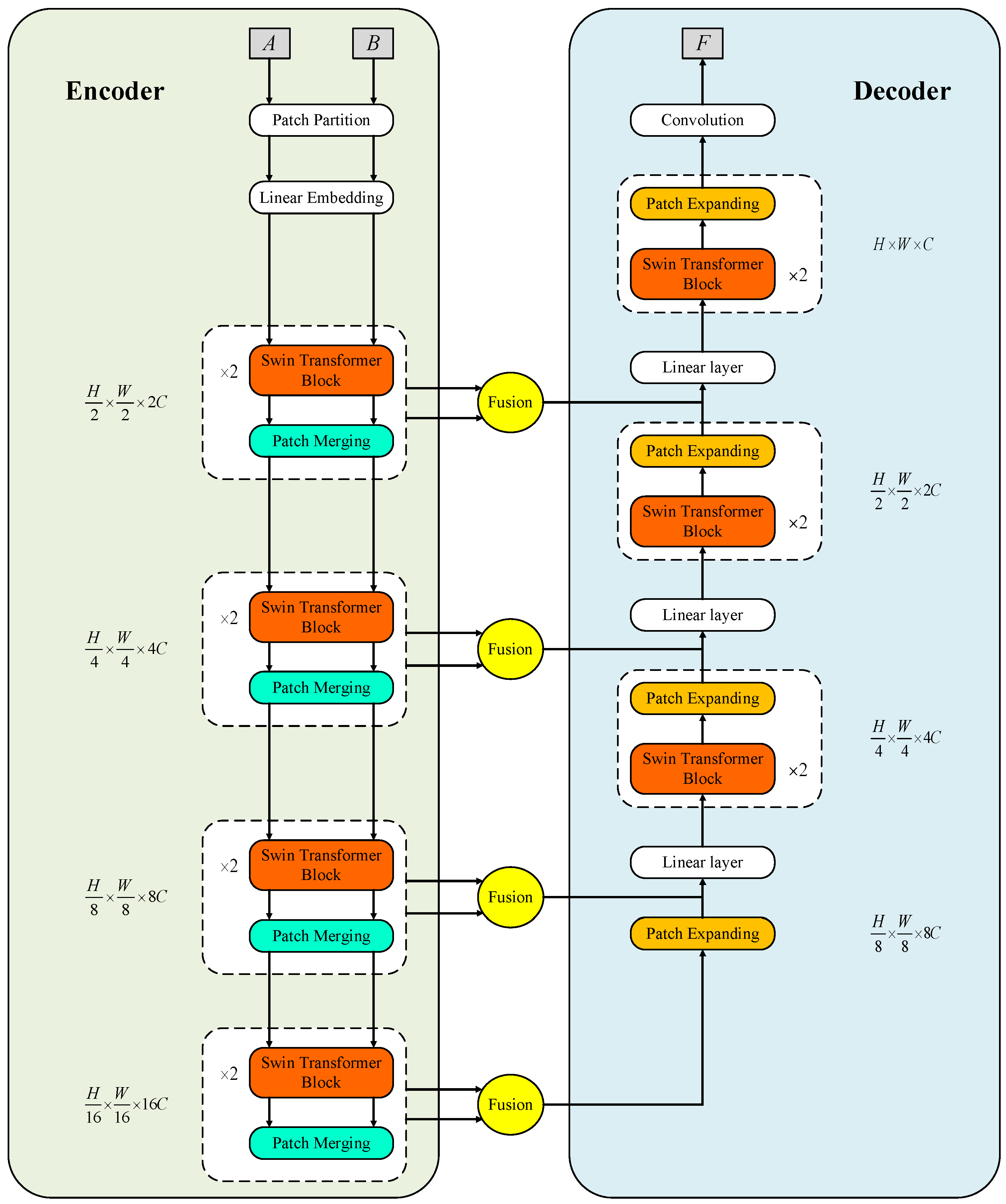
2.2. The Proposed Fusion Method Based on Hainan Gibbon

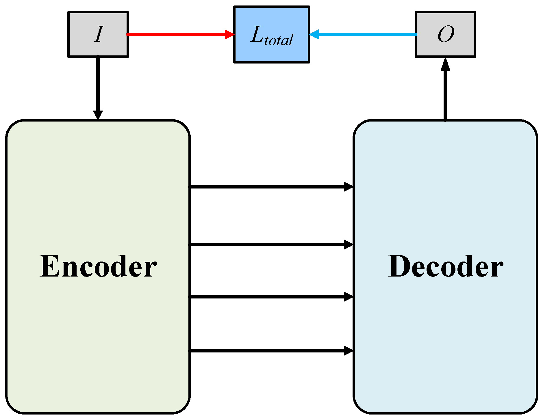
In the complex tropical rainforest environment, the proposed method has stronger representation ability in focusing on infrared Hainan gibbon targets and tropical rainforest details. The proposed method is divided into three sections, as seen in Figure 2: an encoder on the left, a fusion strategy in the middle, and a decoder on the right. A denotes an IR image, B indicates a visible image, and F represents a fused image. Firstly, in the encoder, our algorithm extracts multi-scale features of IR and visible images through Swing Transformer blocks and patch-merging layers [25,26]. Multi-scale deep features can preserve long-distance information. Secondly, the images of different modalities are fused in each scale by a $l_1$-norm based on a row-and-column vector dimension fusion strategy [28]. In the end, a decoder based on the skip connection reconstructs the fused multi-scale features [29].

2.2.1. Encoder

The role of the encoder is to extract multi-scale and long-range semantic features. Suppose that the IR image A and the visible image B are two pre-registered images. In our work, we set $S\in \left\{A,B\right\}$. The input image $S\in {\mathbb{R}}^{H\times W\times C_{in}}$ is initially separated into non-overlapping patches through the patch partition module, and each patch is set as a concatenation of pixel values, where H represents height, W indicates width, and $C_{in}$ refers to the number of channels. Actually, the patch partition module is a $1\times 1$ kernel convolution operation, and it is defined as:

$$\begin{array}{c}\hfill ens{t}_S^0=H_{PP}\left(S\right),\end{array}$$

(1)

where $H_{PP}\left(·\right)$ denotes the patch partition module operation. Then, a linear embedding layer is used to project feature dimension $C_{in}$ into dimension C. Standard Swin Transformer [26] has four architectures, namely Swin-T (Tiny), Swin-S (small), Swin-B (base), and Swin-L (large). The C in Swin-T and Swin-S was set to 96, Swin-B was set to 128, and Swin-L was set to 192. A larger C means larger computational resources. To save computational resources, we set C to 96, i.e., $ens{t}_S^0\in {\mathbb{R}}^{H\times W\times 96}$.

The $ens{t}_S^0$ generates hierarchical feature representations through four stage modules, where each stage module includes two consecutive Swin Transformer blocks and a patch merging layer. Each stage module is calculated as follows:

$$\begin{array}{c}\hfill ens{t}_S^m=H_{P{M}_m}\left(H_{ENST{B}_m}\left(ens{t}_S^{m-1}\right)\right),m=1,2,3,4,\end{array}$$

(2)

$$\begin{array}{c}\hfill H_m,W_m,C_m=\frac{H}{2^m},\frac{W}{2^m},2^{m}C,\end{array}$$

(3)

where $H_{ENST{B}_m}$ denotes the m-th stage Swin Transformer block in the encoder, which aims to extract the long-distance information of the input samples. $H_{P{M}_m}$ indicates the m-th stage patch merging layer, which functions as a double down-sampling of the resolution and extends the output dimension to 2C. Specifically, the patch merging layer splits the input features into four components and concatenates them together. With such a clever design, the feature resolution will be down-sampled by $2\times$ and the feature dimension will be expanded to $2\times$ the original dimension. Deep features are produced at various sizes by combining many layers of Swin Transformer blocks and patch merging layers.

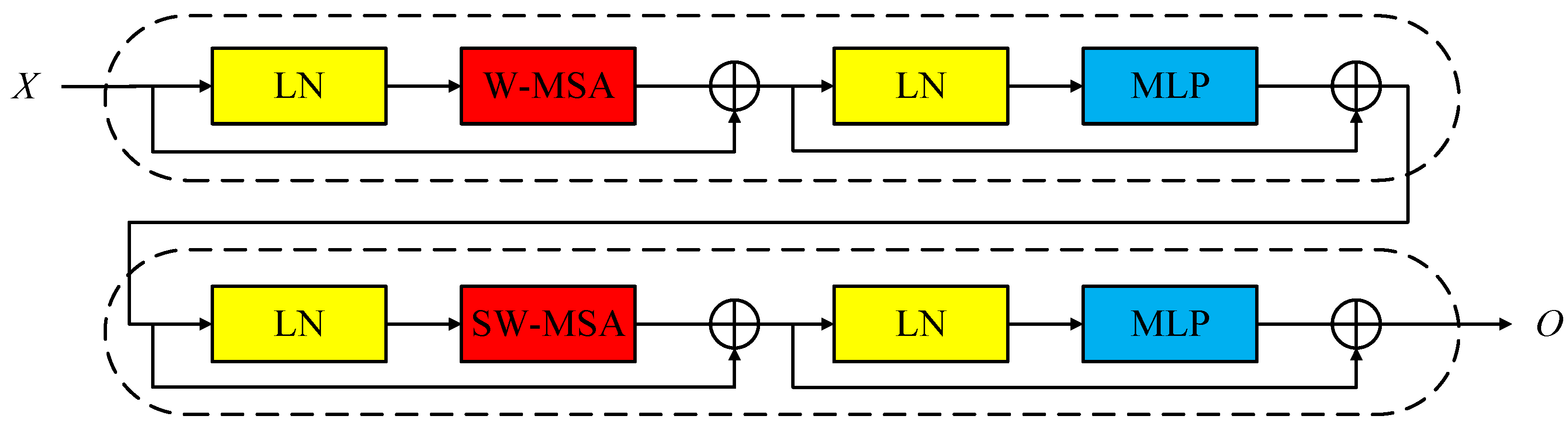
2.2.2. Swin Transformer Block

The Swin Transformer block is a multi-headed self-attention Transformer layer that is based on local attention and shifted window mechanisms [26]. Figure 3 depicts the two successive Swin Transformer blocks’s structural layout, including a windows multi-head self-attention (W-MSA) layer, a shifted windows multi-head self-attention (SW-MSA) layer, four LayerNorm (LN) layers, and two multi-layer perceptron (MLP) layers. A LN layer is employed before each MSA and each MLP, and a residual connection is used after each layer.

For an input sample of size $H\times W\times C$, it is first divided into non-overlapping $M\times M$ local windows and reshaped into $\frac{HW}{M^2}\times M^2\times C$ features, where the total number of windows is $\frac{HW}{M^2}$. Secondly, the corresponding self-attention mechanism is performed in each window. For a local window feature $X\in {\mathbb{R}}^{M^2\times C}$, the query Q, key K, and value V are described below:

$$\begin{array}{c}\hfill Q=X{W}^Q,K=X{W}^K,V=X{W}^V,\end{array}$$

(4)

where $W^Q$, $W^K$, and $W^V$ are learnable projection weight matrices that are shared across different windows.

The computation of the attention mechanism includes the following:

$$\begin{array}{c}\hfill \mathrm{Attention}\left(Q,K,V\right)=\mathrm{SoftMax}\left(\frac{Q{K}^T}{\sqrt{d}}+B\right)V,\end{array}$$

(5)

where B is the learnable relative positional encoding and d is the dimension of keys.

The Swin Transformer block is capable of effectively obtaining global characteristics, and its whole processing is as follows:

$$\begin{array}{c}\hfill \begin{array}{c}X=\mathrm{W}-\mathrm{MSA}\left(\mathrm{LN}\left(X\right)\right)+X\hfill \\ X=\mathrm{MLP}\left(\mathrm{LN}\left(X\right)\right)+X\hfill \\ X=\mathrm{SW}-\mathrm{MSA}\left(\mathrm{LN}\left(X\right)\right)+X\hfill \\ O=\mathrm{MLP}\left(\mathrm{LN}\left(X\right)\right)+X\hfill \end{array}\end{array}$$

(6)

where X denotes the local window of the input and O represents the output.

2.2.3. Fusion Strategy

In our work, a $l_1$-norm based on row and column vector dimensions fusion strategy [28] is used to deal with features of different scales. $ens{t}_S^m\left(i\right)$ and $ens{t}_S^m\left(j\right)$ denote the row vector and column vectors of $ens{t}_S^m\left(i,j\right)$, respectively, where $S\in \left\{A,B\right\}$, $m=1,2,3,4$.

Firstly, the weights of the row vectors of $ens{t}_A^m\left(i\right)$ and $ens{t}_B^m\left(i\right)$ are calculated through the $l_1$-norm, and then their activity level measurements, ${\alpha }_A^m\left(i\right)$ and ${\alpha }_B^m\left(i\right)$, are computed:

$$\begin{array}{c}\hfill {\alpha }_A^m\left(i\right)=\frac{exp\left({∥ens{t}_A^m\left(i\right)∥}_1\right)}{exp\left({∥ens{t}_A^m\left(i\right)∥}_1\right)+exp\left({∥ens{t}_B^m\left(i\right)∥}_1\right)},\end{array}$$

(7)

$$\begin{array}{c}\hfill {\alpha }_B^m\left(i\right)=\frac{exp\left({∥ens{t}_B^m\left(i\right)∥}_1\right)}{exp\left({∥ens{t}_A^m\left(i\right)∥}_1\right)+exp\left({∥ens{t}_B^m\left(i\right)∥}_1\right)},\end{array}$$

(8)

where ${∥·∥}_1$ represents the $l_1$-norm.

Then, the fusion feature $f_{row}^m\left(i,j\right)$ of the row vector dimension is obtained through a weighted-average strategy:

$$\begin{array}{c}\hfill f_{row}^m\left(i,j\right)={\alpha }_A^m\left(i\right)\times ens{t}_A^m\left(i,j\right)+{\alpha }_B^m\left(i\right)\times ens{t}_B^m\left(i,j\right).\end{array}$$

(9)

The fusion strategy of column vector dimension is the same as that of row vector dimension. The activity level measurements ${\beta }_A^m\left(j\right)$ and ${\beta }_B^m\left(j\right)$ of the column vector dimension are calculated by the following formulas:

$$\begin{array}{c}\hfill {\beta }_A^m\left(j\right)=\frac{exp\left({∥ens{t}_A^m\left(j\right)∥}_1\right)}{exp\left({∥ens{t}_A^m\left(j\right)∥}_1\right)+exp\left({∥ens{t}_B^m\left(j\right)∥}_1\right)},\end{array}$$

(10)

$$\begin{array}{c}\hfill {\beta }_B^m\left(j\right)=\frac{exp\left({∥ens{t}_B^m\left(j\right)∥}_1\right)}{exp\left({∥ens{t}_A^m\left(j\right)∥}_1\right)+exp\left({∥ens{t}_B^m\left(j\right)∥}_1\right)}.\end{array}$$

(11)

Then, the fusion feature $f_{col}^m$ of the column vector dimension is obtained through a weighted-average strategy:

$$\begin{array}{c}\hfill f_{col}^m\left(i,j\right)={\beta }_A^m\left(j\right)\times ens{t}_A^m\left(i,j\right)+{\beta }_B^m\left(j\right)\times ens{t}_B^m\left(i,j\right).\end{array}$$

(12)

When $f_{row}^m\left(i,j\right)$ and $f_{col}^m\left(i,j\right)$ are obtained, the final fusion feature $f^m\left(i,j\right)$ is generated by using a specific equation:

$$\begin{array}{c}\hfill f^m\left(i,j\right)=f_{row}^m\left(i,j\right)+f_{col}^m\left(i,j\right).\end{array}$$

(13)

2.2.4. Decoder

The decoder is made up of a patch-expanding layer, three stage modules, and one convolution layer, as illustrated in Figure 2. Each stage module consists of a linear layer, two consecutive Swin Transformer blocks, and a patch-expanding layer. The patch-expanding layer, in contrast to the patch-merging layer, reshapes features of nearby dimensions into a huge feature map with a $2\times$ up-sampling of resolution, and decreases the feature dimension to $1/\phantom{12}2$ of the previous dimension in accordance. In particular, the up-sampled features of the decoder are connected to the corresponding multi-scale fusion features of the encoder through skip connections, with the intention of minimizing the semantic gap between the encoder and decoder, preserving more information from the previous layer to obtain a better fusion result. Since the dimension of the concatenated features after the skip connection is twice that of the original feature, a linear layer is employed to keep the concatenated feature dimension the same as the up-sampled feature dimension. With this architecture, the decoder can utilize the features’ multi-scale structure to its fullest potential.

A detailed description of the algorithmic steps in the decoder is introduced. $f^1$, $f^2$, $f^3$, and $f^4$ refer to fused features at different scales in the encoder, respectively. Firstly, $f^4$ is up-sampled through the patch-expanding layer and concatenated with $f^3$:

$$\begin{array}{c}\hfill des{t}^0=\left[H_{P{E}_1}\left(f^4\right),f^3\right],\end{array}$$

(14)

where $H_{P{E}_1}\left(·\right)$ denotes the first patch-expanding layer in the decoder, $\left[·\right]$ represents the concatenation layer (also known as skip connection), and $des{t}^0\in {\mathbb{R}}^{\frac{H}{8}\times \frac{W}{8}\times 8C}$.

Due to the fact that the dimensions of concatenated features are twice those of the original features, a linear layer is applied to restore the concatenated features to their original dimensions. The first stage module in the decoder is calculated as follows:

$$\begin{array}{c}\hfill ides{t}^1=H_{P{E}_2}\left(H_{DEST{B}_1}\left(L{L}_1\left(des{t}^0\right)\right)\right),\end{array}$$

(15)

$$\begin{array}{c}\hfill des{t}^1=\left[ides{t}^1,f^2\right],\end{array}$$

(16)

where $L{L}_1\left(·\right)$ denotes the first linear layer in the decoder, $H_{DEST{B}_1}\left(·\right)$ indicates the first Swin Transformer block in the decoder, $H_{P{E}_2}\left(.\right)$ represents the second patch-expanding layer in the decoder, and ${\mathit{dest}}^1\in {\mathbb{R}}^{\frac{H}{4}\times \frac{W}{4}\times 4C}$.

The second stage module is calculated as follows:

$$\begin{array}{c}\hfill ides{t}^2=H_{P{E}_3}\left(H_{DEST{B}_2}\left(L{L}_2\left(des{t}^1\right)\right)\right),\end{array}$$

(17)

$$\begin{array}{c}\hfill des{t}^2=\left[ides{t}^2,f^1\right],\end{array}$$

(18)

where $L{L}_2\left(·\right)$ denotes the second linear layer in the decoder, $H_{DEST{B}_2}\left(·\right)$ indicates the second Swin Transformer block in the decoder, $H_{P{E}_3}\left(.\right)$ represents the third patch-expanding layer in the decoder, and ${\mathit{dest}}^2\in {\mathbb{R}}^{\frac{H}{2}\times \frac{W}{2}\times 2C}$.

The third stage module is calculated as follows:

$$\begin{array}{c}\hfill des{t}^3=H_{P{E}_4}\left(H_{DEST{B}_3}\left(L{L}_3\left(des{t}^2\right)\right)\right),\end{array}$$

(19)

$$\begin{array}{c}\hfill F=\mathrm{CONV}\left(des{t}^3\right),\end{array}$$

(20)

where $L{L}_3\left(·\right)$ denotes the third linear layer in the decoder, $H_{DEST{B}_3}\left(·\right)$ indicates the third Swin Transformer block in the decoder, $H_{P{E}_4}\left(.\right)$ represents the fourth patch-expanding layer in the decoder, $\mathrm{CONV}\left(·\right)$ represents convolution operation [24], and F denotes the fused image. It is worth noting that the third-stage module does not have a skip connection.

2.2.5. Loss Function

The training framework of our algorithm is shown in Figure 4. In the training stage, we just consider encoder and decoder networks (the fusion strategy is discarded). After the encoder and decoder weights are fixed, we utilize the fusion strategy to fuse. In order to ensure that the reconstructed image is more similar to the original image, the loss function $L_{total}$ is defined below:

$$\begin{array}{c}\hfill L_{total}=L_{l_1}+\lambda L_{ssim},\end{array}$$

(21)

where $L_{l_1}$ and $L_{ssim}$ represent the $l_1$ loss function and structure similarity (SSIM) [30] loss, respectively, $\lambda$ indicates the trade-off between $L_{l_1}$ and $L_{ssim}$.

The role of $L_{l_1}$ is to make the reconstructed image more similar to the input image. The formula for $L_{l_1}$ is:

$$\begin{array}{c}\hfill L_{l_1}=\frac{1}{HW}\sum \left|O-I\right|,\end{array}$$

(22)

where H is height, W indicates width, I represents input training samples, and O denotes outputs. A smaller $L_{l_1}$ indicates that the input and output images are more similar.

$L_{ssim}$ calculates the structural similarity measurement between the input image and the output image to make the O and the I more similar in structure. $L_{ssim}$ is computed as:

$$\begin{array}{c}\hfill L_{ssim}=1-\mathrm{SSIM}\left(O-I\right),\end{array}$$

(23)

where SSIM $\left(·\right)$ refers to the structural similarity measure [30]. A smaller $L_{ssim}$ indicates that the input and output images are more similar in structure.

The main steps of the proposed IR and visible image fusion method are summarized in Algorithm 1.

Algorithm 1 The proposed infrared and visible image fusion algorithm

Training phase

1. Initialize the networks of Swin-UnetFuse;

2. Update the parameters of networks via minimizing $L_{total}$ according to Equations (21)–(23).

Testing (fusion) phase

Part 1: Encoder

1. Feed infrared image A and visible image B into a series of Swin Transformer blocks and

patch merging layers to generate of different scales features $ens{t}_S^m,m=1,2,3,4,S\in \left\{A,B\right\}$

according to Equations (1)–(3);

Part 2: Fusion strategy

2. Perform $l_1$-norm based on row and column vector dimensions fusion strategy to $ens{t}_A^m$ and

$ens{t}_B^m$ to generate $f^m$ according to Equations (7)–(13);

Part 3: Decoder

3. Perform up-sampling and concatenating operation to generate $des{t}^0$ according to Equation (14);

4. Perform a series of linear layers, Swin Transformer blocks, patch expanding layers and

concatenation layers to generate $des{t}^3$ according to Equations (15)–(19);

5. Feed the $des{t}^3$ into the convolution operation to generate the result F according to Equation (20).

3. Experiments and Discussion

The section includes five parts: the first part introduces the infrared and visible dataset of Hainan gibbons that we photographed; the second part is about experimental setups; the third part describes the evaluation metrics of images; the fourth part is three ablation studies; and a comparison of our approach and other approaches is shown in the final part.

3.1. Infrared and Visible Dataset of Hainan Gibbons

There are currently 37 Hainan gibbons in 5 social groups (groups A, B, C, D, and E). The object of our observation was group C, which has only eight Hainan gibbons: three subadults (one 3-year-old, one 5-year-old, and one 6-year-old) and five adults (9–16 years old) [9]. In order to observe and study the Hainan gibbons, our team took a large number of infrared and visible photos of the life of Hainan gibbons in Hainan Bawangling National Nature Reserve by using an infrared camera and a visible camera in the drone [31]. The drone, model Dajiang Innovation (DJI) Mavic 2 Enterprise Advanced, is equipped with a quadcopter and a three-axis stabilization system. The infrared camera adopts an Uncooled VOx Microbolometer sensor with a resolution of $640\times 512$, and a spectral band of 8–14 $\mathsf{\mu }\mathrm{m}$. The visible camera adopts a $1/\phantom{12^{\prime \prime }}{2}^{\prime \prime }$ CMOS sensor with 48 million pixels, and a maximum image size of $8000\times 6000$.

When a drone approaches a gibbon, it may cause the gibbon to avoid the drone. In order not to disturb the gibbons, we determined threshold flight distances for both above-canopy and within-understory drone flights that would not cause any disturbance to gibbons while still being able to collect clear images. We chose 30 m above the canopy and 20 m in the understory as the flight distance for surveys. The gibbons did not respond to the drone at these two threshold distances, but when we flew the drone closer, the gibbons left. Therefore, we chose these two threshold distances as the flight parameters, and the flights did not cause any disturbance to the gibbons.

We selected 21 pairs of IR and visible images as the test images, converted each pair of images to grayscale, and registered them according to [32]. Figure 5 shows four pairs of testing images.

3.2. Experimental Setups

In the training stage, we trained the Swin-UetFuse with 5000 images from the MS-COCO dataset [33], and each image was converted to a size of $224\times 224$ and a grayscale range of −1 to 1. For our approach, we set $1\times 1$ for the patch size and $7\times 7$ for the sliding window size. Furthermore, we selected Adam as the optimizer and set the following parameters: $1\times {10}^{-5}$ for learning rate, 2 for batch size, and 2 for epoch. The head numbers of the four Swin Transformer blocks in the encoder were set to 3, 6, 12, and 24, respectively. The head numbers of the three Transformer blocks in the decoder were set to 6, 12, and 24, respectively.

In the fusion stage, we converted the grayscale range of test images to −1 and 1 and applied the sliding window $224\times 224$ to partition them into several patches, where the value of invalid region is filled with 0. After the combination of each patch pair, we conducted the reverse operation according to the previous partition order to obtain the fusion image. The experimental environments of our method were Intel Core i7 11700, RAM 64G, NVIDIA GeForce RTX 3070 8 GB and PyTorch.

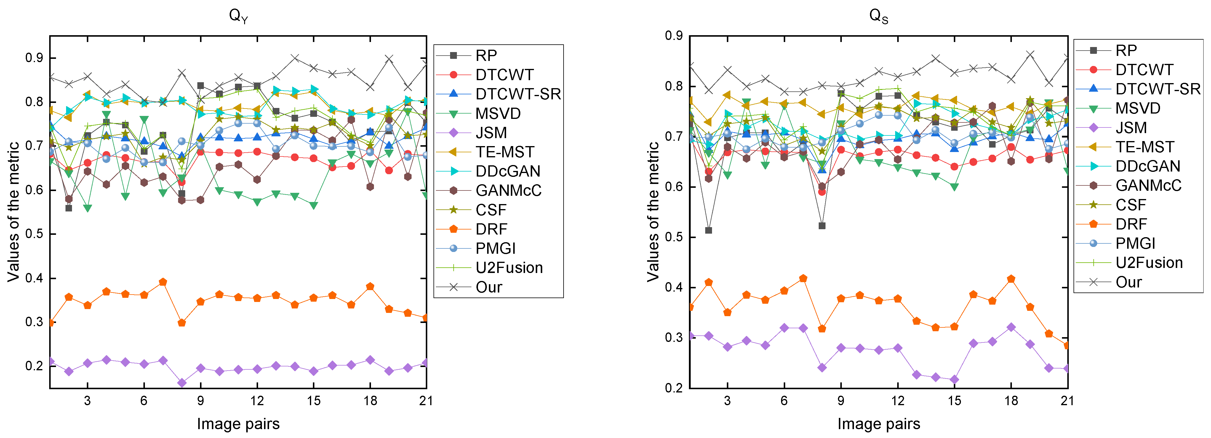
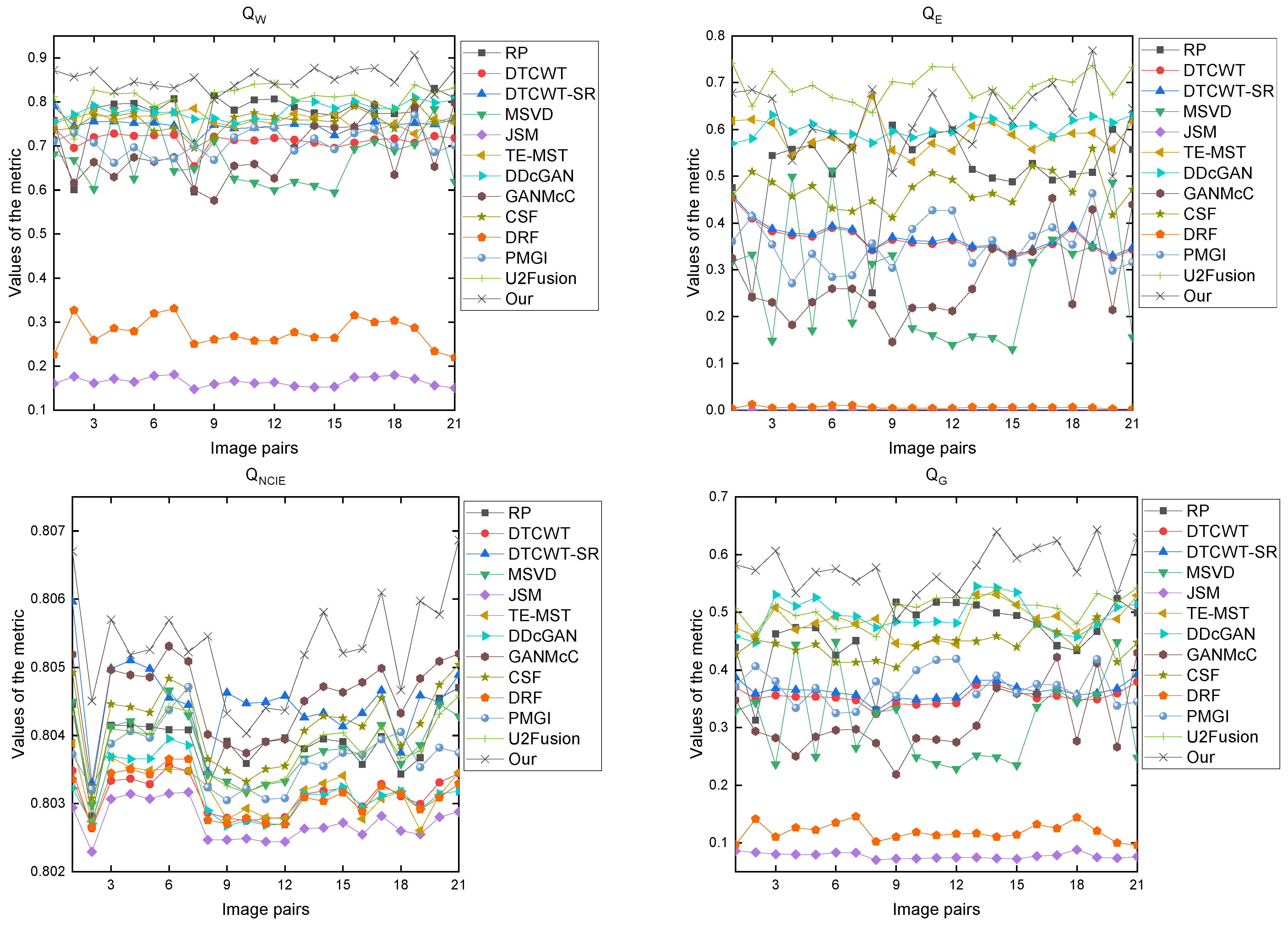
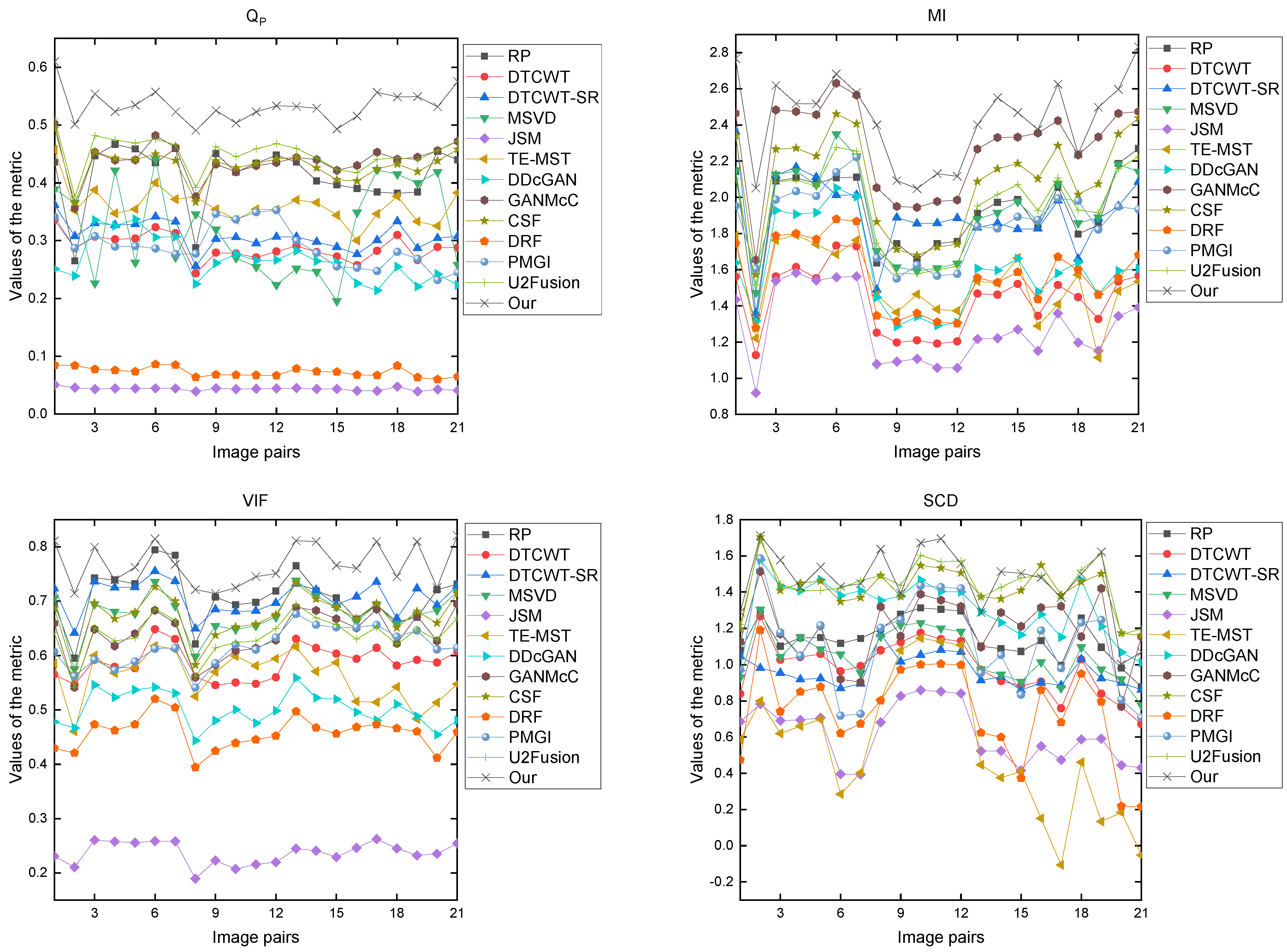
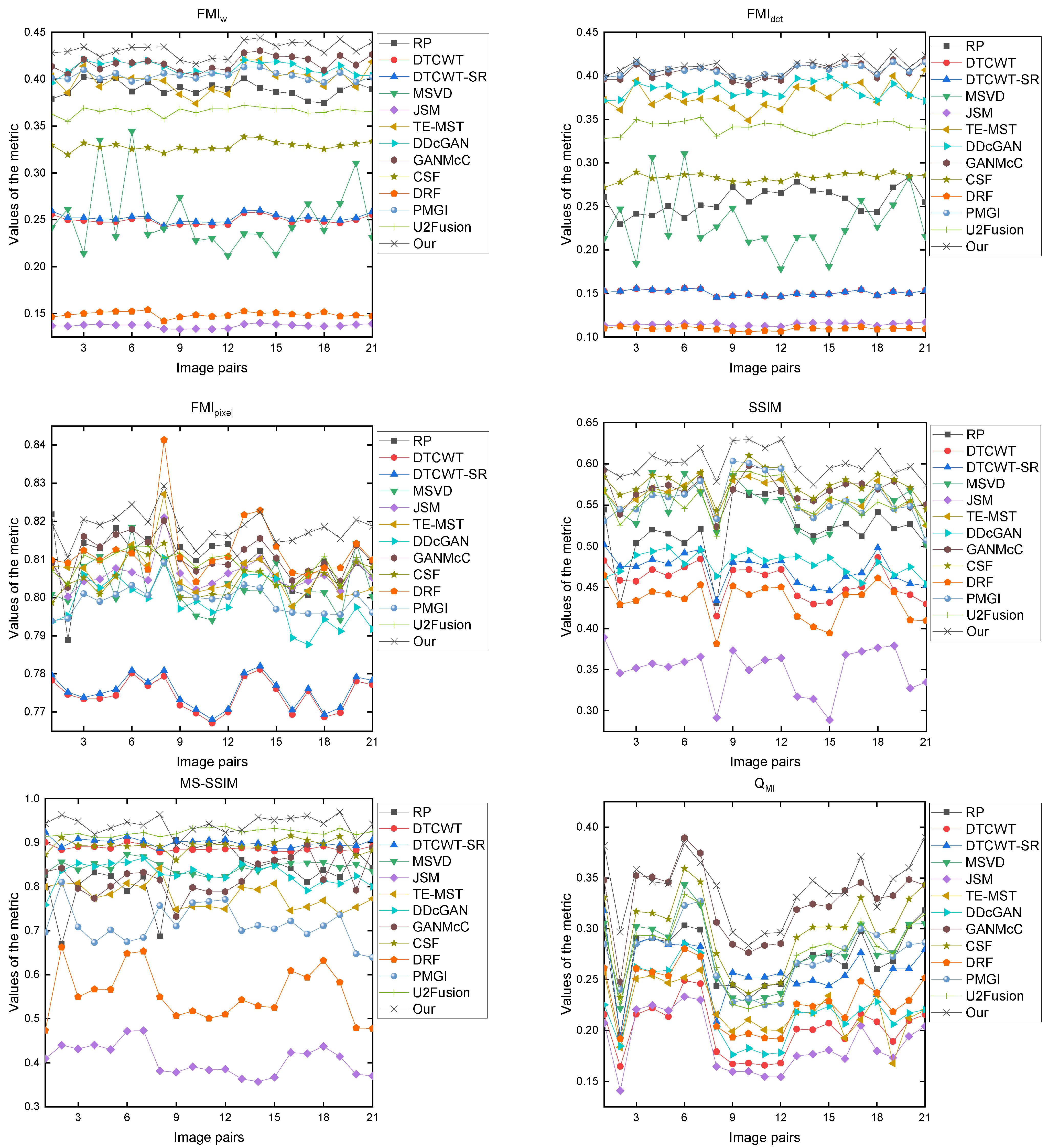
3.3. Image Fusion Evaluation

Image fusion evaluation includes subjective evaluation and objective evaluation. The subjective evaluation of a fused image is done with the use of human vision, including color, brightness, definition, contrast, noise, fidelity, etc. The subjective evaluation is essentially to judge whether the fused image gives a satisfactory feeling.

In order to comprehensively evaluate the image fusion performance, we selected 16 significant objective evaluation metrics to assess the fusion performance: $FM{I}_w$, $FM{I}_{dct}$ and $FM{I}_{pixel}$ [34], structural similarity index measure ($SSIM$) [30], the multi-scale structural similarity ($MS-SSIM$) [35], normalized mutual information ($Q_{MI}$) [36], Yang’s metric ($Q_Y$) [37], Piella’s three metrics ($Q_S$, $Q_W$, $Q_E$) [38], nonlinear correlation information entropy ($Q_{NCIE}$) [39], gradient-based metric ($Q_G$) [40], phase-congruency-based metric ($Q_P$) [41], mutual information ($MI$) [42], visual information fidelity ($VIF$) [43], sum of the correlations of differences ($SCD$) [44]. In all metrics, larger values demonstrate better fusion performance.

3.4. Ablation Studies

In this section, we performed three ablation studies: the ablation study of the parameter $\lambda$ in the loss function, the skip connection ablation study, and the multiple scales ablation study. We adopted 21 pairs of images as test images and used the above-mentioned 16 evaluation metrics as the reference standard for fusion performance. If an algorithm obtains more optimal values, its fusion performance will be stronger.

3.4.1. The Ablation Study of the Parameter $\lambda$ in the Loss Function

In this ablation study, we set $\lambda =10$, $\lambda =100$, $\lambda =1000$, and $\lambda$ = 10,000, respectively. All other parameters were the same.

Table 1. The average values of different $\lambda$ methods.

Method	${\mathit{FMI}}_{\mathit{w}}$	${\mathit{FMI}}_{\mathit{dct}}$	${\mathit{FMI}}_{\mathit{pixel}}$	$\mathit{SSIM}$	$\mathit{MS}-\mathit{SSIM}$	${\mathit{Q}}_{\mathit{MI}}$	${\mathit{Q}}_{\mathit{Y}}$	${\mathit{Q}}_{\mathit{S}}$	${\mathit{Q}}_{\mathit{W}}$	${\mathit{Q}}_{\mathit{E}}$	${\mathit{Q}}_{\mathit{NCIE}}$	${\mathit{Q}}_{\mathit{G}}$	${\mathit{Q}}_{\mathit{P}}$	$\mathit{MI}$	$\mathit{VIF}$	$\mathit{SCD}$
10	0.3626	0.3797	0.7980	0.5551	0.8501	0.2760	0.6625	0.6900	0.7161	0.3621	0.8038	0.3258	0.3807	1.9280	0.6557	1.2981
100	0.4239	0.4017	0.8107	0.5924	0.9073	0.3153	0.7989	0.7868	0.8005	0.5066	0.8047	0.5254	0.4934	2.2362	0.7199	1.2902
1000	0.4317	0.4100	0.8185	0.6010	0.9413	0.3396	0.8494	0.8210	0.8523	0.6272	0.8053	0.5765	0.5339	2.4336	0.7677	1.4630
10,000	0.4175	0.3932	0.8077	0.5927	0.9158	0.3200	0.8198	0.7990	0.8167	0.5386	0.8048	0.5416	0.4907	2.2820	0.7315	1.3487

displays the various metrics’ average values. Bold typefaces are used to denote the best results. When $\lambda =1000$, the model obtained 16 optimal values. Therefore, in the later experiments, we set $\lambda$ to 1000.

3.4.2. The Skip Connection Ablation Study

In the comparison experiment, we removed all skip connections, and all other settings were the same.

Table 2. The average values of different methods.

Method	${\mathit{FMI}}_{\mathit{w}}$	${\mathit{FMI}}_{\mathit{dct}}$	${\mathit{FMI}}_{\mathit{pixel}}$	$\mathit{SSIM}$	$\mathit{MS}-\mathit{SSIM}$	${\mathit{Q}}_{\mathit{MI}}$	${\mathit{Q}}_{\mathit{Y}}$	${\mathit{Q}}_{\mathit{S}}$	${\mathit{Q}}_{\mathit{W}}$	${\mathit{Q}}_{\mathit{E}}$	${\mathit{Q}}_{\mathit{NCIE}}$	${\mathit{Q}}_{\mathit{G}}$	${\mathit{Q}}_{\mathit{P}}$	$\mathit{MI}$	$\mathit{VIF}$	$\mathit{SCD}$
Without skip connection	0.1850	0.1439	0.7845	0.4875	0.7958	0.2169	0.5471	0.5999	0.6010	0.1656	0.8031	0.2320	0.1535	1.4842	0.5467	0.6338
Skip connection	0.4317	0.4100	0.8185	0.6010	0.9413	0.3396	0.8494	0.8210	0.8523	0.6272	0.8053	0.5765	0.5339	2.4336	0.7677	1.4630

displays the various metrics’ average values. Bold typefaces are used to denote the best results. The table demonstrates that the approach with the skip connections achieved better fusion performance due to the fact that the skip connections compensate for the spatial loss of down-sampling and preserve more information from the encoder.

3.4.3. The Multiple Scales Ablation Study

We explored the effect of multiple scales on fusion performance. In the comparison experiment, we removed all patch-merging layers, patch-expanding layers, and linear layers. All other settings were the same.

Table 3. The average values of different methods.

Method	${\mathit{FMI}}_{\mathit{w}}$	${\mathit{FMI}}_{\mathit{dct}}$	${\mathit{FMI}}_{\mathit{pixel}}$	$\mathit{SSIM}$	$\mathit{MS}-\mathit{SSIM}$	${\mathit{Q}}_{\mathit{MI}}$	${\mathit{Q}}_{\mathit{Y}}$	${\mathit{Q}}_{\mathit{S}}$	${\mathit{Q}}_{\mathit{W}}$	${\mathit{Q}}_{\mathit{E}}$	${\mathit{Q}}_{\mathit{NCIE}}$	${\mathit{Q}}_{\mathit{G}}$	${\mathit{Q}}_{\mathit{P}}$	$\mathit{MI}$	$\mathit{VIF}$	$\mathit{SCD}$
Without multiple scales	0.4362	0.4115	0.8143	0.6045	0.9156	0.3479	0.7997	0.7859	0.8006	0.5216	0.8052	0.5221	0.5066	2.4631	0.7185	1.3999
Multiple scales	0.4317	0.4100	0.8185	0.6010	0.9413	0.3396	0.8494	0.8210	0.8523	0.6272	0.8053	0.5765	0.5339	2.4336	0.7677	1.4630

displays the various metrics’ average values. Bold typefaces are used to denote the best results. The table shows that the multiscale model obtained 11 best values, indicating that the multi-scale model has better fusion performance. This is because the model reconstructs the source images by fusing images of different scales, so the fusion results obtained a more natural visual experience.

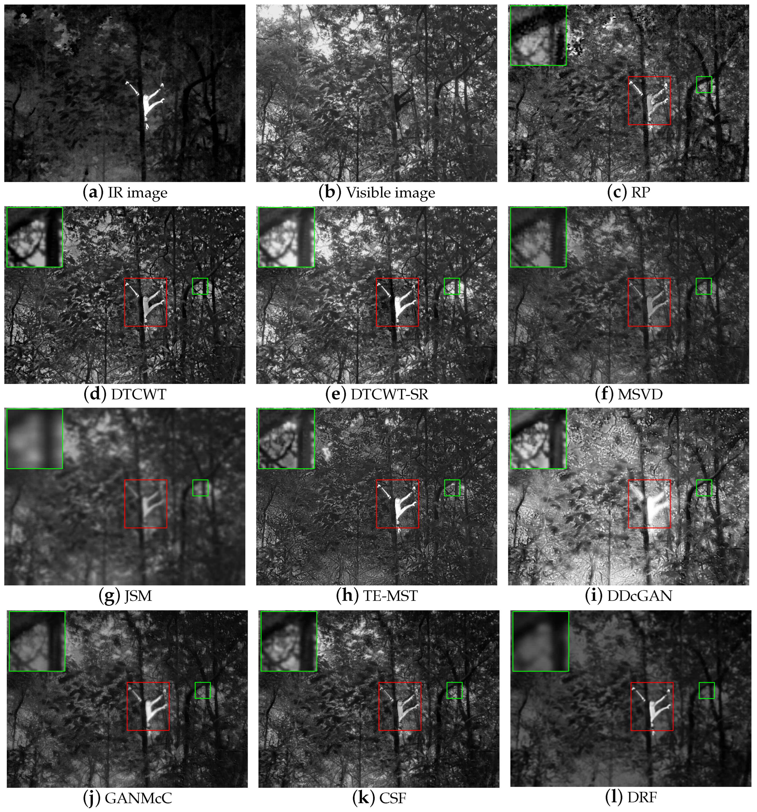
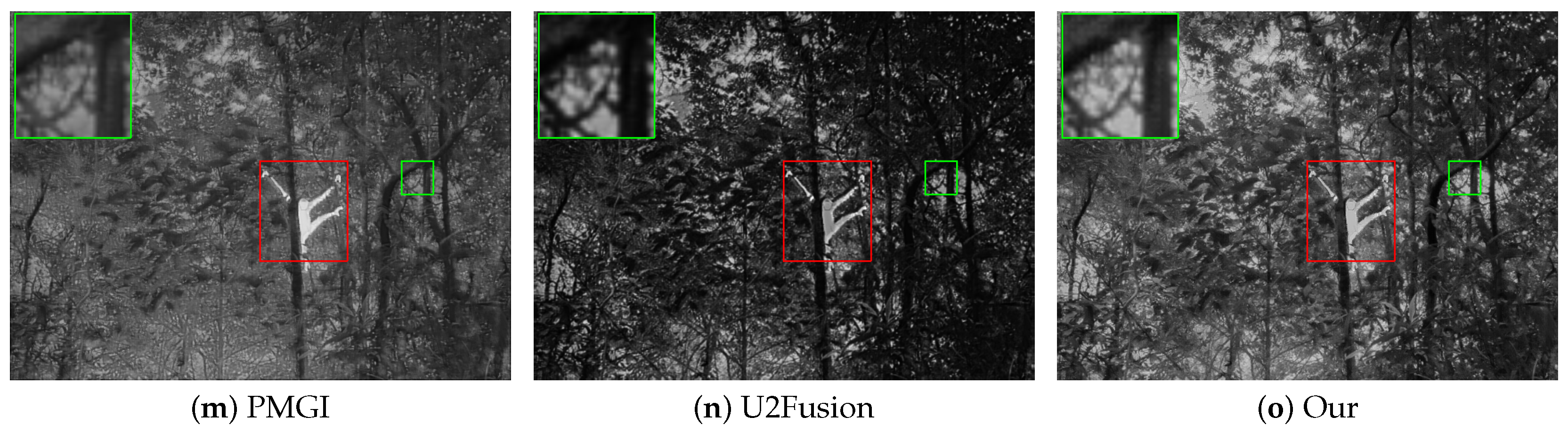
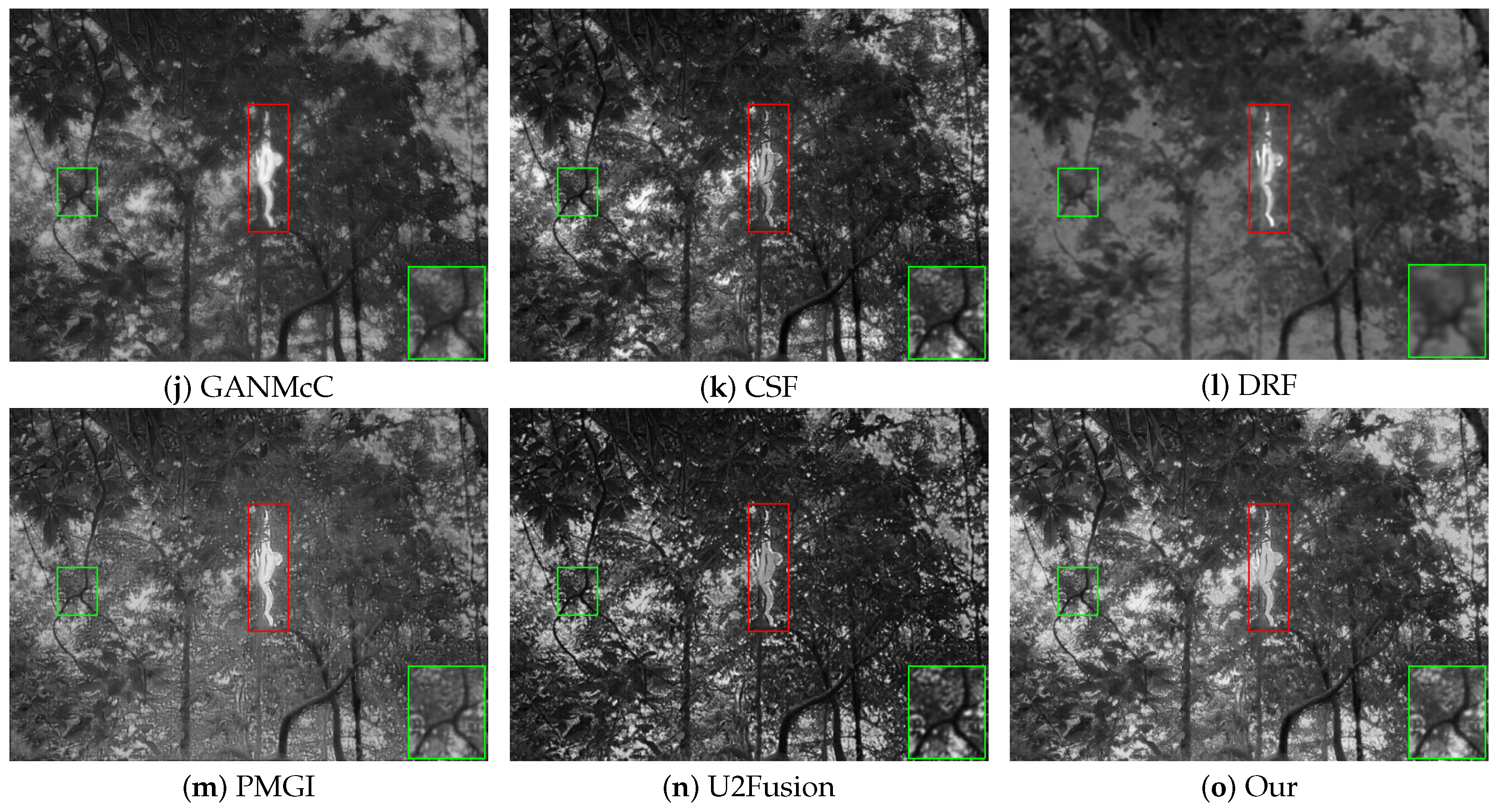
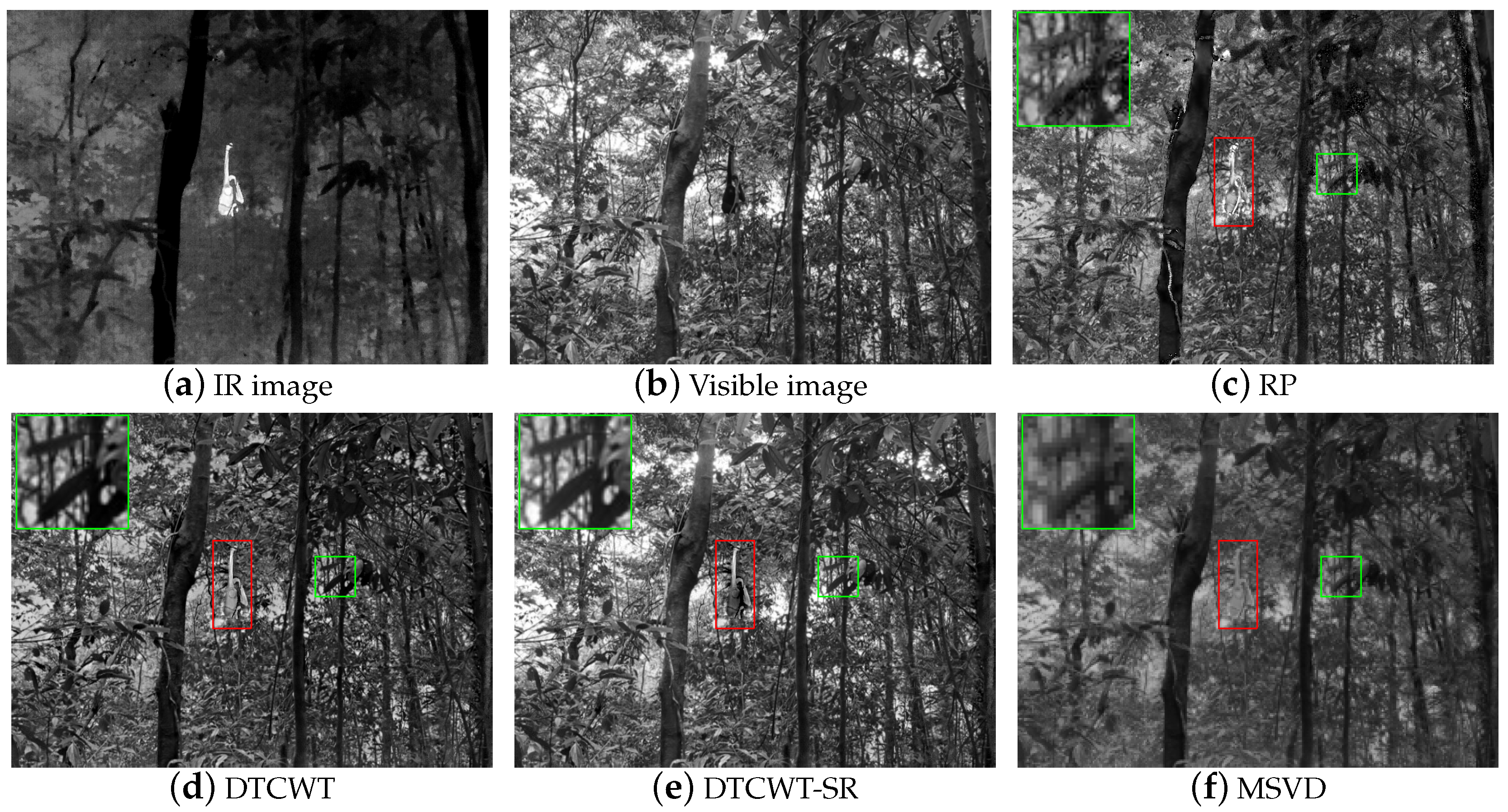
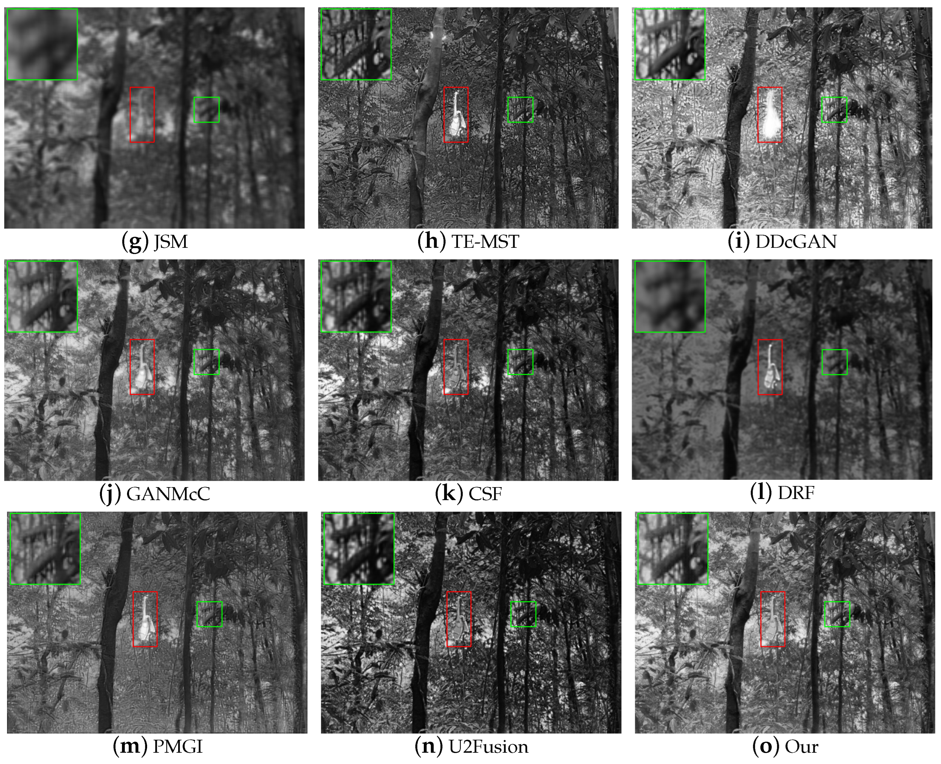
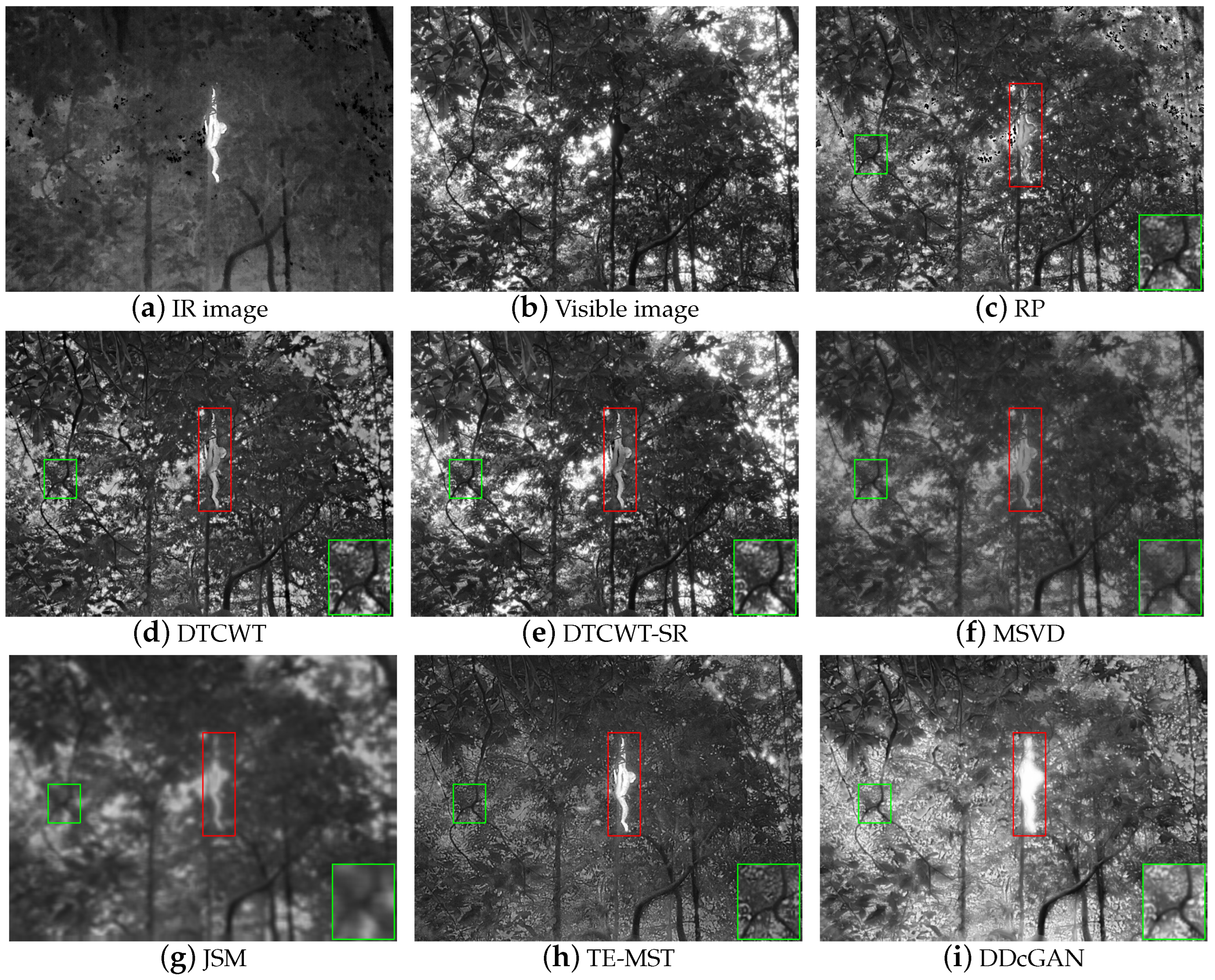
3.5. Experimental Results and Discussion

We selected twelve representative competitive algorithms to compare with ours in terms of subjective and objective evaluation. These twelve comparison algorithms included RP [45], DTCWT [46], DTCWT-SR [47], MSVD [48], JSM [49], TE-MST [50], DDcGAN [16], GANMcC [17], CSF [20], DRF [21], PMGI [18], and U2Fusion [19]. The corresponding parameter settings in the comparison algorithms were set to the default values given by their authors. It is worth noting that these comparison algorithms are based on ordinary IR and visible image fusion methods rather than the method developed by Hainan gibbons. This is because our method is the first one developed for Hainan gibbons. Figure 6, Figure 7 and Figure 8 show three representative examples of fusion results. A few areas of the fusion results have been magnified for easier reference.

In Figure 6, the drone’s infrared and visible cameras capture a Hainan gibbon hanging on a tree. The IR image amply displays the gibbon’s thermal radiation data, but the tropical rainforest in the background is blurred. The visible image vividly depicts the features of the tropical rainforest; however, it is difficult to capture useful information about the gibbon. The best fusion result for this case would be to clearly capture background features while also collecting thermal radiation information from the gibbon. The tropical rainforests in the RP and MSVD results introduce some noise (as shown in the green boxes in Figure 6c,f). Although the DTCWT and TE-MST approaches achieve good fusion results, the tropical rainforests in their backgrounds lack some details (see Figure 6d,h). As a classic fusion method, the DTCWT-SR method achieves good fusion performance in this example (see Figure 6e). The tropical rainforests in the JSM and DRF results are clearly blurred (as shown in the green boxes in Figure 6g,l). The fusion result based on the DDcGAN technique looks overexposed (as shown in Figure 6i). The GANMCC and U2Fusion techniques introduce too much infrared spectrum, causing their results to look too dark (as shown in Figure 6j,n). The tropical rainforests in the CSF and PMGI schemes lack some details (see the tropical rainforests in Figure 6k,m). The proposed approach well extracts the information about the Hainan gibbon’s thermal radiation and the tropical rainforest’s details with a more natural visual experience (as shown in the boxes in Figure 6o).

In Figure 7, the drone’s infrared and visible cameras capture a Hainan gibbon preparing to jump. The Hainan gibbons in the fusion results of RP, DTCWT, DTCWT-SR, and MSVD lose a lot of energy, resulting in unnatural visual effects (see gibbons in Figure 7c–f). The Hainan gibbon and tropical rainforest in the JSM-based approach are fuzzy (see Figure 7g). Although the TE-MST technique emphasizes the Hainan gibbon, the tropical rainforest loses some details, giving rise to an abnormal visual sensation (as shown in the tropical rainforest in Figure 7h). The result of DDcGAN is overexposed (as shown in Figure 7i). Although the Hainan gibbons in the GANMCC and DRF results are high brightness, the tropical rainforests in their results are fuzzy (see the tropical rainforest in Figure 7j,l). This is because these two methods introduce excessive infrared spectra. In addition, the Hainan gibbons in the CSF and U2Fusion algorithms are low-brightness (see gibbons in Figure 7k,n). The PMGI approach achieves a great fusion result, but the tropical rainforest lacks some details (as shown in the tropical rainforest in Figure 7m). Compared with other approaches, our approach has a high-brightness Hainan gibbon and clear tropical rainforest details (as shown in the boxes in Figure 7o).

In Figure 8, the drone’s infrared and visible cameras capture a Hainan gibbon hanging on a tree by one hand. The Hainan gibbons in RP, DTCWT, and DTCWT-SR approaches introduce lots of noise, resulting in unnatural visual perception (see the gibbons in Figure 8c–e). The tropical rainforests in the MSVD and JSM models are clearly blurred (see green boxes in Figure 8f,g). The TE-MST algorithm achieves good fusion, but the rainforest lacks some details. The DDcGAN technique is overexposed. The tropical rainforests in GANMCC, DRF, and PMGI results are missing a large number of details (see the green boxes in Figure 8j,l,m). The CSF and U2Fusion approaches introduce too much infrared spectrum, leading the Hainan gibbons in their images to suffer from low brightness and contrast (as shown in the gibbons in Figure 8k,n). Our method locates the gibbon well and has clear background details (as shown in the boxes in Figure 8o).

Figure 9 and Figure 10 show the evaluation metrics of each pair of testing images. For better observation,

Table 4. The average values of different methods.

Method	${\mathit{FMI}}_{\mathit{w}}$	${\mathit{FMI}}_{\mathit{dct}}$	${\mathit{FMI}}_{\mathit{pixel}}$	$\mathit{SSIM}$	$\mathit{MS}-\mathit{SSIM}$	${\mathit{Q}}_{\mathit{MI}}$	${\mathit{Q}}_{\mathit{Y}}$	${\mathit{Q}}_{\mathit{S}}$	${\mathit{Q}}_{\mathit{W}}$	${\mathit{Q}}_{\mathit{E}}$	${\mathit{Q}}_{\mathit{NCIE}}$	${\mathit{Q}}_{\mathit{G}}$	${\mathit{Q}}_{\mathit{P}}$	$\mathit{MI}$	$\mathit{VIF}$	$\mathit{SCD}$
RP	0.3896	0.2567	0.8094	0.5200	0.8309	0.2714	0.7453	0.7059	0.7721	0.5118	0.8039	0.4649	0.4132	1.9215	0.7074	1.1432
DTCWT	0.2496	0.1511	0.7745	0.4567	0.8877	0.2007	0.6694	0.6612	0.7133	0.3651	0.8031	0.3536	0.2887	1.4343	0.5872	0.9799
DTCWT-SR	0.2522	0.1512	0.7755	0.4718	0.9005	0.2606	0.7169	0.6969	0.7480	0.3691	0.8045	0.3636	0.3095	1.9059	0.7066	0.9616
MSVD	0.2519	0.2303	0.8030	0.5500	0.8446	0.2772	0.6425	0.6784	0.6673	0.2734	0.8038	0.3107	0.3213	1.9276	0.6768	1.0470
JSM	0.1370	0.1147	0.8062	0.3496	0.4070	0.1872	0.1993	0.2764	0.1646	0.0002	0.8027	0.0774	0.0435	1.2778	0.2369	0.6169
TE-MST	0.3997	0.3767	0.8061	0.5605	0.7792	0.2208	0.7934	0.7611	0.7587	0.5860	0.8032	0.4837	0.3614	1.5199	0.5611	0.5390
DDcGAN	0.4116	0.3830	0.7988	0.4787	0.8285	0.2203	0.7916	0.7212	0.7808	0.6027	0.8032	0.4945	0.2660	1.6030	0.5017	1.3101
GANMcC	0.4170	0.4050	0.8110	0.5673	0.8240	0.3260	0.6634	0.6891	0.6833	0.2757	0.8046	0.3131	0.4395	2.2785	0.6397	1.1982
CSF	0.3286	0.2834	0.8051	0.5766	0.8934	0.2976	0.7233	0.7287	0.7559	0.4710	0.8042	0.4419	0.4305	2.0935	0.6726	1.4168
DRF	0.1492	0.1095	0.8123	0.4332	0.5559	0.2301	0.3474	0.3636	0.2756	0.0057	0.8031	0.1188	0.0729	1.5634	0.4572	0.7395
PMGI	0.4036	0.4065	0.7994	0.5574	0.7134	0.2724	0.7021	0.7022	0.7066	0.3521	0.8037	0.3715	0.2906	1.8591	0.6162	1.1040
U2Fusion	0.3662	0.3414	0.8085	0.5558	0.9234	0.2775	0.7544	0.7406	0.8064	0.6934	0.8039	0.5057	0.4512	1.9436	0.6375	1.4455
Our	0.4317	0.4100	0.8185	0.6010	0.9413	0.3396	0.8494	0.8210	0.8523	0.6272	0.8053	0.5765	0.5339	2.4336	0.7677	1.4630

displays the various methods’ average values. Bold typefaces are used to denote the best results. In Table 4, it can be seen that our method achieved the best results among all other metrics except for $Q_E$. $Q_E$ is a fusion quality metric based on image edge dependence. The larger the $Q_E$, the better the fusion performance. U2Fusion is an excellent fusion algorithm and achieved the best score in the $Q_E$ metric.

Overall, none of the 12 comparison methods performed the fusion task well, and all had some drawbacks. Figure 6, Figure 7, Figure 8, Figure 9 and Figure 10 and Table 4 show that the Swin-UetFuse had better fusion performance than the 12 comparison methods. This is because the Swin-UetFuse has a powerful global and long-range semantic information extraction capability, and the capability is very suitable for application in complex tropical rainforest environments. The Swin-UetFuse technology provides an important reference for the observation and protection of the Hainan gibbons.

4. Conclusions

In the article, we propose a fusion method of IR and visible images based on Hainan gibbon for the first time, termed Swin-UetFuse. The Swin-UetFuse is a U-shaped encoder-decoder structure with skip connections, which aims to extract global and long-range semantic information. The skip connections reduce the semantic gap between the encoder and decoder, preserving more information from the previous layer. We used 21 pairs of Hainan gibbon dataset to perform experiments, and the experimental results demonstrate that the proposed method achieves excellent fusion performance. The IR and visible image fusion technology of drones provides an important reference for the observation and protection of the Hainan gibbon. In future work, we will design the Swin UetFuse technology into a cell phone application that fuses IR and visible images from drones in real time, so that the fused images can better discriminate between Hainan gibbons and other creatures. In addition, there are other state-protected animals in Hainan Bawangling Nature Reserve, such as Hainan peacock-pheasant (Polyplectron katsumatae), Hainan partridge (Arborophila ardens), and water monitor (Varanus salvator). In future work, we will apply the Swin-UetFuse technology to other animals.

References

1. Estrada, A.; Garber, P.A.; Rylands, A.B.; Roos, C.; Fernandez-Duque, E.; Di Fiore, A.; Nekaris, K.A.I.; Nijman, V.; Heymann, E.W.; Lambert, J.E.; et al. Impending extinction crisis of the world’s primates: Why primates matter. Sci. Adv. 2017, 3, e1600946. [Google Scholar] [CrossRef] [PubMed]
2. IUCN. The IUCN Red List of Threatened Species; Version 2019-2. 2019. Available online: http://www.iucnredlist.org (accessed on 10 July 2023).
3. Zhang, Y.; Yu, J.; Lin, S.; He, J.; Xu, Y.; Tu, J.; Jiang, H. Spatiotemporal variation of anthropogenic drivers predicts the distribution dynamics of Hainan gibbon. Glob. Ecol. Conserv. 2023, 43, e02472. [Google Scholar] [CrossRef]
4. Wang, X.; Wen, S.; Niu, N.; Wang, G.; Long, W.; Zou, Y.; Huang, M. Automatic detection for the world’s rarest primates based on a tropical rainforest environment. Glob. Ecol. Conserv. 2022, 38, e02250. [Google Scholar] [CrossRef]
5. Turvey, S.T.; Bryant, J.V.; Duncan, C.; Wong, M.H.; Guan, Z.; Fei, H.; Ma, C.; Hong, X.; Nash, H.C.; Chan, B.P.; et al. How many remnant gibbon populations are left on Hainan? Testing the use of local ecological knowledge to detect cryptic threatened primates. Am. J. Primatol. 2017, 79, e22593. [Google Scholar] [CrossRef]
6. Dufourq, E.; Durbach, I.; Hansford, J.P.; Hoepfner, A.; Ma, H.; Bryant, J.V.; Stender, C.S.; Li, W.; Liu, Z.; Chen, Q.; et al. Automated detection of Hainan gibbon calls for passive acoustic monitoring. Remote Sens. Ecol. Conserv. 2021, 7, 475–487. [Google Scholar] [CrossRef]
7. Chan, B.P.L.; Lo, Y.F.P.; Hong, X.J.; Mak, C.F.; Ma, Z. First use of artificial canopy bridge by the world’s most critically endangered primate the Hainan gibbon Nomascus hainanus. Sci. Rep. 2020, 10, 15176. [Google Scholar] [CrossRef]
8. Rahman, D.A.; Sitorus, A.B.Y.; Condro, A.A. From Coastal to Montane Forest Ecosystems, Using Drones for Multi-Species Research in the Tropics. Drones 2021, 6, 6. [Google Scholar] [CrossRef]
9. Zhang, H.; Wang, C.; Turvey, S.T.; Sun, Z.; Tan, Z.; Yang, Q.; Long, W.; Wu, X.; Yang, D. Thermal infrared imaging from drones can detect individuals and nocturnal behavior of the world’s rarest primate. Glob. Ecol. Conserv. 2020, 23, e01101. [Google Scholar] [CrossRef]
10. Degollada, E.; Amigó, N.; O’Callaghan, S.A.; Varola, M.; Ruggero, K.; Tort, B. A Novel Technique for Photo-Identification of the Fin Whale, Balaenoptera physalus, as Determined by Drone Aerial Images. Drones 2023, 7, 220. [Google Scholar] [CrossRef]
11. Jiménez-Torres, M.; Silva, C.P.; Riquelme, C.; Estay, S.A.; Soto-Gamboa, M. Automatic Recognition of Black-Necked Swan (Cygnus melancoryphus) from Drone Imagery. Drones 2023, 7, 71. [Google Scholar] [CrossRef]
12. Povlsen, P.; Linder, A.C.; Larsen, H.L.; Durdevic, P.; Arroyo, D.O.; Bruhn, D.; Pertoldi, C.; Pagh, S. Using Drones with Thermal Imaging to Estimate Population Counts of European Hare (Lepus europaeus) in Denmark. Drones 2022, 7, 5. [Google Scholar] [CrossRef]
13. Keshet, D.; Brook, A.; Malkinson, D.; Izhaki, I.; Charter, M. The Use of Drones to Determine Rodent Location and Damage in Agricultural Crops. Drones 2022, 6, 396. [Google Scholar] [CrossRef]
14. Zhang, A.; Li, Z.; Zang, R.; Liu, S.; Long, W.; Chen, Y.; Liu, S.; Liu, H.; Qi, X.; Feng, Y.; et al. Food plant diversity in different-altitude habitats of Hainan gibbons (Nomascus hainanus): Implications for conservation. Glob. Ecol. Conserv. 2022, 38, e02204. [Google Scholar] [CrossRef]
15. Du, Y.; Li, D.; Yang, X.; Peng, D.; Tang, X.; Liu, H.; Li, D.; Hong, X.; Song, X. Reproductive phenology and its drivers in a tropical rainforest national park in China: Implications for Hainan gibbon (Nomascus hainanus) conservation. Glob. Ecol. Conserv. 2020, 24, e01317. [Google Scholar] [CrossRef]
16. Ma, J.; Xu, H.; Jiang, J.; Mei, X.; Zhang, X.P. DDcGAN: A dual-discriminator conditional generative adversarial network for multi-resolution image fusion. IEEE Trans. Image Process. 2020, 29, 4980–4995. [Google Scholar] [CrossRef]
17. Ma, J.; Zhang, H.; Shao, Z.; Liang, P.; Xu, H. GANMcC: A generative adversarial network with multiclassification constraints for infrared and visible image fusion. IEEE Trans. Instrum. Meas. 2020, 70, 1–14. [Google Scholar] [CrossRef]
18. Zhang, H.; Xu, H.; Xiao, Y.; Guo, X.; Ma, J. Rethinking the image fusion: A fast unified image fusion network based on proportional maintenance of gradient and intensity. Proc. AAAI Conf. Artif. Intell. 2020, 34, 12797–12804. [Google Scholar] [CrossRef]
19. Xu, H.; Ma, J.; Jiang, J.; Guo, X.; Ling, H. U2Fusion: A unified unsupervised image fusion network. IEEE Trans. Pattern Anal. Mach. Intell. 2020, 44, 502–518. [Google Scholar] [CrossRef]
20. Xu, H.; Zhang, H.; Ma, J. Classification saliency-based rule for visible and infrared image fusion. IEEE Trans. Comput. Imaging 2021, 7, 824–836. [Google Scholar] [CrossRef]
21. Xu, H.; Wang, X.; Ma, J. DRF: Disentangled representation for visible and infrared image fusion. IEEE Trans. Instrum. Meas. 2021, 70, 1–13. [Google Scholar] [CrossRef]
22. Li, S.; Zou, Y.; Wang, G.; Lin, C. Infrared and visible image fusion method based on principal component analysis network and multi-scale morphological gradient. Infrared Phys. Technol. 2023, 133, 104810. [Google Scholar] [CrossRef]
23. Li, S.; Zou, Y.; Wang, G.; Lin, C. Infrared and Visible Image Fusion Method Based on a Principal Component Analysis Network and Image Pyramid. Remote Sens. 2023, 15, 685. [Google Scholar] [CrossRef]
24. LeCun, Y.; Bottou, L.; Bengio, Y.; Haffner, P. Gradient-based learning applied to document recognition. Proc. IEEE 1998, 86, 2278–2324. [Google Scholar] [CrossRef]
25. Cao, H.; Wang, Y.; Chen, J.; Jiang, D.; Zhang, X.; Tian, Q.; Wang, M. Swin-unet: Unet-like pure transformer for medical image segmentation. In Proceedings of the Computer Vision—ECCV 2022 Workshops, Tel Aviv, Israel, 23–27 October 2022; pp. 205–218. [Google Scholar]
26. Liu, Z.; Lin, Y.; Cao, Y.; Hu, H.; Wei, Y.; Zhang, Z.; Lin, S.; Guo, B. Swin transformer: Hierarchical vision transformer using shifted windows. In Proceedings of the IEEE/CVF International Conference on Computer Vision, Montreal, BC, Canada, 11–17 October 2021; pp. 10012–10022. [Google Scholar]
27. Long, W.; Zang, R.; Ding, Y. Air temperature and soil phosphorus availability correlate with trait differences between two types of tropical cloud forests. Flora-Morphol. Distrib. Funct. Ecol. Plants 2011, 206, 896–903. [Google Scholar] [CrossRef]
28. Wang, Z.; Chen, Y.; Shao, W.; Li, H.; Zhang, L. SwinFuse: A Residual Swin Transformer Fusion Network for Infrared and Visible Images. arXiv 2022, arXiv:2204.11436. [Google Scholar] [CrossRef]
29. Ronneberger, O.; Fischer, P.; Brox, T. U-net: Convolutional networks for biomedical image segmentation. In Proceedings of the 18th International Conference of the Medical Image Computing and Computer-Assisted Intervention (MICCAI 2015), Munich, Germany, 5–9 October 2015; pp. 234–241. [Google Scholar]
30. Wang, Z.; Bovik, A.C.; Sheikh, H.R.; Simoncelli, E.P. Image quality assessment: From error visibility to structural similarity. IEEE Trans. Image Process. 2004, 13, 600–612. [Google Scholar] [CrossRef]
31. Zhang, H.; Turvey, S.T.; Pandey, S.P.; Song, X.; Sun, Z.; Wang, N. Commercial drones can provide accurate and effective monitoring of the world’s rarest primate. Remote Sens. Ecol. Conserv. 2023. early view. [Google Scholar] [CrossRef]
32. Li, J.; Hu, Q.; Ai, M. RIFT: Multi-modal image matching based on radiation-variation insensitive feature transform. IEEE Trans. Image Process. 2019, 29, 3296–3310. [Google Scholar] [CrossRef]
33. Lin, T.Y.; Maire, M.; Belongie, S.; Hays, J.; Perona, P.; Ramanan, D.; Dollár, P.; Zitnick, C.L. Microsoft coco: Common objects in context. In European Conference on Computer Vision; Springer: Berlin/Heidelberg, Germany, 2014; pp. 740–755. [Google Scholar]
34. Haghighat, M.; Razian, M.A. Fast-FMI: Non-reference image fusion metric. In Proceedings of the 2014 IEEE 8th International Conference on Application of Information and Communication Technologies (AICT), Astana, Kazakhstan, 15–17 October 2014; pp. 1–3. [Google Scholar]
35. Ma, K.; Zeng, K.; Wang, Z. Perceptual quality assessment for multi-exposure image fusion. IEEE Trans. Image Process. 2015, 24, 3345–3356. [Google Scholar] [CrossRef]
36. Hossny, M.; Nahavandi, S.; Creighton, D. Comments on ’Information measure for performance of image fusion’. Electron. Lett. 2008, 44, 1066–1067. [Google Scholar] [CrossRef]
37. Yang, C.; Zhang, J.Q.; Wang, X.R.; Liu, X. A novel similarity based quality metric for image fusion. Inf. Fusion 2008, 9, 156–160. [Google Scholar] [CrossRef]
38. Piella, G.; Heijmans, H. A new quality metric for image fusion. In Proceedings of the 2003 International Conference on Image Processing (Cat. No. 03CH37429), Barcelona, Spain, 14–17 September 2003; Volume 3, p. III–173. [Google Scholar]
39. Wang, Q.; Shen, Y.; Jin, J. Performance evaluation of image fusion techniques. Image Fusion Algorithms Appl. 2008, 19, 469–492. [Google Scholar]
40. Xydeas, C.; Petrovic, V. Objective image fusion performance measure. Electron. Lett. 2000, 36, 308–309. [Google Scholar] [CrossRef]
41. Zhao, J.; Laganiere, R.; Liu, Z. Performance assessment of combinative pixel-level image fusion based on an absolute feature measurement. Int. J. Innov. Comput. Inf. Control 2007, 3, 1433–1447. [Google Scholar]
42. Qu, G.; Zhang, D.; Yan, P. Information measure for performance of image fusion. Electron. Lett. 2002, 38, 1. [Google Scholar] [CrossRef]
43. Sheikh, H.R.; Bovik, A.C. Image information and visual quality. IEEE Trans. Image Process. 2006, 15, 430–444. [Google Scholar] [CrossRef]
44. Aslantas, V.; Bendes, E. A new image quality metric for image fusion: The sum of the correlations of differences. Aeu-Int. J. Electron. Commun. 2015, 69, 1890–1896. [Google Scholar] [CrossRef]
45. Toet, A. Image fusion by a ratio of low-pass pyramid. Pattern Recognit. Lett. 1989, 9, 245–253. [Google Scholar] [CrossRef]
46. Lewis, J.J.; O’Callaghan, R.J.; Nikolov, S.G.; Bull, D.R.; Canagarajah, N. Pixel-and region-based image fusion with complex wavelets. Inf. Fusion 2007, 8, 119–130. [Google Scholar] [CrossRef]
47. Liu, Y.; Liu, S.; Wang, Z. A general framework for image fusion based on multi-scale transform and sparse representation. Inf. Fusion 2015, 24, 147–164. [Google Scholar] [CrossRef]
48. Naidu, V. Image fusion technique using multi-resolution singular value decomposition. Def. Sci. J. 2011, 61, 479. [Google Scholar] [CrossRef]
49. Gao, Z.; Zhang, C. Texture clear multi-modal image fusion with joint sparsity model. Optik 2017, 130, 255–265. [Google Scholar] [CrossRef]
50. Chen, J.; Li, X.; Luo, L.; Mei, X.; Ma, J. Infrared and visible image fusion based on target-enhanced multiscale transform decomposition. Inf. Sci. 2020, 508, 64–78. [Google Scholar] [CrossRef]
Figure 1. An example of infrared and visible image fusion in a Hainan gibbon.
Drones 07 00543 g001
Figure 2. The structure of Swin-UnetFuse.
Drones 07 00543 g002
Figure 3. The architecture of two successive Swin Transformer blocks.
Drones 07 00543 g003
Figure 4. The Swin-UnetFuse training model in this paper.
Drones 07 00543 g004
Figure 5. Illustrations of four pairs of testing images.
Drones 07 00543 g005
Figure 6. Fusion results of the first pair of source images.
Drones 07 00543 g006aDrones 07 00543 g006b
Figure 7. Fusion results of the second pair of source images.
Drones 07 00543 g007aDrones 07 00543 g007b
Figure 8. Fusion results of the third pair of source images.
Drones 07 00543 g008aDrones 07 00543 g008b
Figure 9. Objective comparisons of the eight metrics, i.e., F M I w , F M I d c t , F M I p i x e l , S S I M , M S S S I M , Q M I , Q Y , and Q S .
Drones 07 00543 g009aDrones 07 00543 g009b
Figure 10. Objective comparisons of the eight metrics, i.e., Q W , Q E , Q N C I E , Q G , Q P , M I , V I F , and S C D .
Drones 07 00543 g010aDrones 07 00543 g010b