Abstract
Rubber tree is one of the essential tropical economic crops, and rubber tree powdery mildew (PM) is the most damaging disease to the growth of rubber trees. Accurate and timely detection of PM is the key to preventing the large-scale spread of PM. Recently, unmanned aerial vehicle (UAV) remote sensing technology has been widely used in the field of agroforestry. The objective of this study was to establish a method for identifying rubber trees infected or uninfected by PM using UAV-based multispectral images. We resampled the original multispectral image with 3.4 cm spatial resolution to multispectral images with different spatial resolutions (7 cm, 14 cm, and 30 cm) using the nearest neighbor method, extracted 22 vegetation index features and 40 texture features to construct the initial feature space, and then used the SPA, ReliefF, and Boruta–SHAP algorithms to optimize the feature space. Finally, a rubber tree PM monitoring model was constructed based on the optimized features as input combined with KNN, RF, and SVM algorithms. The results show that the simulation of images with different spatial resolutions indicates that, with resolutions higher than 7 cm, a promising classification result (>90%) is achieved in all feature sets and three optimized feature subsets, in which the 3.4 cm resolution is the highest and better than 7 cm, 14 cm, and 30 cm. Meanwhile, the best classification accuracy was achieved by combining the Boruta–SHAP optimized feature subset and SVM model, which were 98.16%, 96.32%, 95.71%, and 88.34% at 3.4 cm, 7 cm, 14 cm, and 30 cm resolutions, respectively. Compared with SPA–SVM and ReliefF–SVM, the classification accuracy was improved by 6.14%, 5.52%, 12.89%, and 9.2% and 1.84%, 0.61%, 1.23%, and 6.13%, respectively. This study’s results will guide rubber tree plantation management and PM monitoring.
1. Introduction
The natural rubber produced by the rubber tree is known as one of the four major industrial raw materials, along with steel, coal, and oil, and is the only renewable resource among them. Rubber trees are widely planted in the tropical areas of Asia, Africa, Oceania, and Latin America [1], among which China has planted more than 11,000 km² of rubber trees [2]. Powdery mildew (PM) is the main infectious disease of rubber trees, caused by Oidium heveae B.A (OH) Steinmann, and it has been widely distributed in all rubber-growing countries since the disease was first detected in Java, Indonesia, in 1918 [3]. PM can reduce the photosynthesis of rubber tree leaves and slow down the growth rate of rubber trees, and when the infection is severe, it causes secondary leaf drop on rubber trees, leading to a delayed harvesting period and reduced natural rubber yield by up to 45% [4,5]. Some studies have shown that the rate of natural rubber yield loss is highly correlated with the severity of PM [6]. Current traditional detection methods for PM in rubber trees are based on visual diagnosis and polymerase chain reaction (PCR) diagnosis. However, visual diagnosis is inefficient and time-consuming, and although PCR is the most reliable detection method, it requires specialized equipment and personnel [7,8]. The shortcomings of these methods make it difficult to guide rubber tree disease management accurately, so a rapid and economical method to detect the disease is urgently needed.
Remote sensing technology has provided an important technical solution for large-area, rapid, and accurate monitoring of crop pests and diseases. Santoso et al. [9] explored the possibility of using QuickBird satellite imagery to detect basal stem rot disease. Zhang et al. [10] used the PlanetScope satellite to acquire multi-temporal, high-resolution remote sensing images to monitor the occurrence and development of pine wilt disease. However, satellite optical images are often affected by bad weather such as clouds, rain, and fog during the imaging process, making it difficult to acquire usable remote sensing images in a timely manner. Compared with satellite platforms, unmanned aerial vehicle (UAV) platforms have been widely used for crop disease monitoring with the advantages of low cost and short revisit cycles [11]. Pádua et al. [12] used the crop height model (CHM) to segment individual canopies on UAV multispectral images for multi-temporal analysis of chestnut ink disease and nutrient deficiency in chestnut trees by extracting vegetation indices and spectral bands. Yang et al. [13] constructed the hail vegetation index (HGVI) and ratio vegetation index (RVI) to identify cotton hail damage based on the red band and near-infrared band of UAV multispectral images, respectively. The results showed that both HGVI and RVI were more than 90% accurate, and kappa coefficients were above 0.85 at different sampling fields. In general, vegetation index (VI) features are more sensitive to internal physiological changes in leaves caused by diseases, while texture features (TF) are sensitive to external morphological changes in leaves [14]. Therefore, many studies have also improved the ability to represent diseases by combining spectral and texture features.
In recent years, the scale problem has become a hotspot of remote sensing research, and the selection of appropriate spatial resolution images for agricultural monitoring can improve the crop monitoring area and reduce the cost of operation. Ye et al. [15] analyzed the effect of classification of banana Fusarium wilt at different spatial resolutions (0.5 m, 1 m, 2 m, 5 m, and 10 m resolution), and the results showed that good identification accuracy of Fusarium wilt was obtained when the resolution was higher than 2 m. As the resolution decreased, the identification accuracy of Fusarium wilt showed a decreasing trend. Wei et al. [16] analyzed the effect on wheat lodging identification at different spatial resolutions (1.05 cm, 2.09 cm, and 3.26 cm), and found that the classification accuracy could be effectively improved by selecting appropriate spatial resolutions and classification models. Meanwhile, an appropriate feature optimization method can not only achieve the purpose of data reduction and improve the accuracy of the model, but also ensure the stability, robustness, and high generalization ability of the model. Zhao et al. [17] selected 15 potential vegetation indices based on UAV multispectral images and used the minimal redundancy maximal relevance (MRMR) algorithm to select three sensitive spectral features for the construction of an areca yellow leaf disease classification model, ensuring the maximum relevance of the feature while removing the advantage of redundant features. Ma et al. [18] used analysis of variance (ANOVA) and successive projection algorithm (SPA) to extract sensitive vegetation index features and texture features of forest trees with different damage levels to improve the generalization ability of the Erannis jacobsoni Djak severity model. In addition, the appropriate choice of data analysis method is very important, as it directly affects the reliability and accuracy of the results. Narmilan et al. [19] examined white leaf disease in sugarcane using four ML algorithms: XGBoost (XGB), Random Forest (RF), Decision Tree (DT), and K-Nearest Neighbors (KNN). The results showed that the XGB, RF, and KNN models all achieved an overall accuracy (OA) of more than 94% in detecting white leaf disease. Rodríguez et al. [20] proposed a UAV-based multispectral image assessment and detection method for potato late blight, evaluating the performance of five machine learning algorithms: RF (OA = 84.2%), Gradient Boosting Classifier (GBC) (OA = 77.7%), SVM (OA = 86.9%), LSVM (OA = 87.5%), and KNN (OA = 80.6%).
The above studies show that UAV remote sensing technology provides a fast and effective way to monitor crop pests and diseases. In this study, we used UAV multispectral images and accurate ground truth data as data sources, and different feature selection methods (SPA, ReliefF, and Boruta–SHAP) to extract sensitive spectral and texture features at different image spatial resolutions (3.4 cm, 7 cm, 14 cm, and 30 cm) combined with KNN, SVM, and RF algorithms to construct PM monitoring models. Our research objectives are (1) to evaluate the effects of different image spatial resolutions on the classification accuracy of rubber tree PM, (2) to explore the best classification method for UAV multispectral images, and (3) to build a rubber tree PM monitoring model in different spatial resolution images using suitable feature selection methods and classification methods. The results will provide guidance for rubber tree PM management.
2. Materials and Methods
2.1. Study Area
PM occurs mainly in spring when rubber trees are in the leaf-extraction stage and OH infects the living host cells of young leaves or buds, resulting in defoliation of young leaves and discoloration and curling of the margins of old leaves [21], as shown in Figure 1. At the beginning, when the young leaves are infected with the disease, radial silvery-white mycelium appears on the leaf surface or leaf back. With the development of the disease, a layer of white powdery material appears on the spots, forming white powdery spots of various sizes. When the disease turns serious, the front and back of the diseased leaf are covered with white powder, and the leaf displays crinkled deformation and yellowing, and can easily fall off.
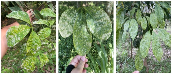
Figure 1.
The symptoms of rubber tree powdery mildew.
The experiment was performed from 25 to 27 April 2022 at the rubber forest study area of the Chinese Academy of Tropical Agricultural Sciences in Danzhou City, Hainan Province (109°28′30″ E, 19°32′40″ N), as shown in Figure 2. The total area of the study area was about 14,720 m2, with 648 rubber trees planted in 26 rows with a spacing of 3 m and a row spacing of 7.3 m. The height of the trees was about 12–15 m, and the rubber tree species was RY73397.
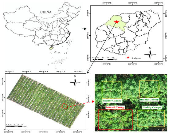
Figure 2.
Location of the study area.
2.2. Data Acquisition and Processing
2.2.1. UAV Multispectral Image Acquisition
Multispectral image data was acquired by a DJI Phantom 4 multispectral (P4M) drone with a real-time kinematic (RTK) module attached to it. The multispectral imaging system consists of one visible (RGB) camera and five multispectral cameras (blue, green, red, red edge, and near-infrared bands). The main parameters are listed in Table 1.

Table 1.
Main parameters of the DJI Phantom 4 multispectral drone.
The flight at the site of the study area was conducted between 12:00 p.m. and 13:00 p.m. on 25 April 2022, with clear and cloudless weather. In mapping, the setting of UAV flight parameters is critical in obtaining stable image data. DJI GS Pro software was used for route planning, and the UAV flight plan parameters were set to a flight height of 60 m, a flight speed of 4.2 m/s, 80% frontal overlap rate, and 70% side overlap rate. Multispectral images were acquired by taking photos at equal time intervals, and the total duration of the mission was 8 min and 22 s. The resolution of the multispectral image acquired was 3.4 cm/pixel. Figure 3a shows the flight route of the UAV aerial photography mission performed in the study area, Figure 3b shows the DJI Phantom 4 multispectral (P4M) used to acquire multispectral images, and Figure 3c shows the diffuse reflectance board for radiometric calibration.

Figure 3.
(a) Flight route (green line) and parameters, (b) DJI Phantom 4 multispectral (P4M), (c) Diffuse reflectance board (right).
2.2.2. Ground Truth Data Collection
Ground observation data was collected on 25–26 April 2022. To ensure the reliability of the observed data, a combination of telescopic high branch shears, mechanical rising ladder, and visual observations by UAV was used for ground observation, as shown in Figure 4a–c. Specifically, firstly, experts visually inspected the trees by drones, then collected leaves for identification with high branch shears and a mechanical rising ladder, and finally recorded the locations of the canopy that showed either healthy or PM symptoms by a handheld D-RTK2 high-precision GNSS mobile station, which provides highly accurate positioning (horizontal precision of 0.01 m).
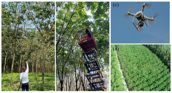
Figure 4.
(a) Telescopic high branch shears, (b) mechanical rising ladder, (c) P4M, (d) rubber plantation.
In this paper, the classification criterion used is the percentage of infected PM leaf area to the total leaf area of the canopy. If the percentage of infected PM leaf area to the total leaf area of the canopy was less than 5%, the canopy was considered healthy, otherwise it was considered diseased (with a canopy consisting of a diameter of 30–50 cm containing 30–40 leaves). Finally, we labeled 526 canopy samples from 153 rubber trees, including 271 healthy samples and 255 diseased samples. Then, these sample data were divided into a training set (75%) and a validation set (25%).
2.2.3. Data Preprocessing
A total of 1200 multispectral images were acquired by DJI Phantom 4 multispectral (P4M). Two-dimensional multispectral reconstruction was performed using DJI Terra software (version 3.3.4; DJI Inc., Shenzhen, China), including image stitching, geometric correction, and radiometric correction. The radiometric correction allows the conversion of each pixel value (defined as Digital Number (DN)) into radiance, which is the amount of radiation coming from the surface affected by solar radiation [22]. Specifically, we collected the calibration images before the flight using two standard reflectance panels with the reflectance of 0.25 and 0.5, as shown in Figure 3c. Afterward, the calibration parameters of the calibration images were extracted using the new radiometric calibration tool in DJI Terra software, the calibration parameters were used to pre-process the DN values of each image during the 2D multispectral reconstruction, and the corrected multispectral image data were finally generated. Meanwhile, in order to evaluate the effect of classification accuracy of images with different spatial resolutions, we chose to resample the original multispectral image of 3.4 cm and use the nearest neighbor resampling algorithm to generate multispectral images with resolutions of 7 cm, 14 cm, and 30 cm. This method is widely used because of its fast implementation and simplicity [23], and the value of the output pixel is determined by the center of the nearest pixel on the input grid, which is more suitable for classification tasks. It has been widely used in the field of UAV-based crop monitoring for multiple scale crop simulations, such as wheat yellow rust [14], banana wilt [15], and citrus greening disease [24].
2.3. Feature Extraction of Multispectral Images
2.3.1. Extraction of Vegetation Index (VI) and Texture Features (TF)
Vegetation indices have been widely used in UAV remote sensing disease monitoring. The infection of rubber tree leaves with PM leads to internal physiological and biochemical changes, such as suppression of photosynthesis, reduction of chlorophyll content, and decrease of water content [25]. In this study, we selected 22 vegetation indices related to crop diseases from the crop disease monitoring literature as candidate spectral features, as shown in Table 2. Rubber trees infected with PM also have changes in external morphology, such as the appearance of powdery mildew patches on the front or back of leaves, leaves turning yellow, wilt, and other symptoms. Gray-Level Co-Occurrence Matrix (GLCM) [26], introduced by Haralick for texture feature extraction, is a common method to describe texture by the study of spatial correlation properties of gray levels. In this study, we selected eight commonly used TFs as candidate texture features, including Mean (Mea), Variance (Var), Homogeneity (Hom), Contrast (Con), Dissimilarity (Dis), Entropy (Ent), Second Moment (Sec), and Correlation (Cor). The GLCM tool in ENVI 5.3 software was utilized to extract the GLCM values for five bands (40 texture features in total) in the multispectral image, and specifically by extracting the average GLCM texture values for four offsets ([0, 1], [1, 1], [0, 1], [1, −1]) in the image through the 3 × 3 pixel sliding window.

Table 2.
Candidate vegetation indices extracted from UAV multispectral images.
2.3.2. Feature Selection
A total of 22 vegetation index features and 40 texture features were extracted from the multispectral images as candidate features for constructing the rubber tree PM classification model. Due to the large number of candidate features, it was necessary to perform correlation analysis and feature selection on the selected VIs and TFs features to remove redundant features. The successive projections algorithm (SPA) [41] is a forward selection algorithm, where the principle of selecting variables is first to select an initial variable and then add a new variable with the lowest information redundancy at each iteration. It reduces the fitting complexity in the model building process and speeds up the fitting operation by ensuring the minimum covariance between the selected features. The main principle of the ReliefF algorithm [42] is to randomly select a sample R from the training sample set each time and then to find out k-nearest neighbor samples from the sample set of the same type of R. After that, k-nearest neighbor samples are found from the sample set that are not of the same type, multiple sample points are constantly randomly selected for updating the feature weights to obtain the feature weight ordering, and finally the effective features are selected by setting the threshold value.
Boruta–SHAP is a wrapper feature selection method that combines the Boruta feature selection algorithm with Shapley values [43]. SHAP values show the importance of each feature in the model prediction, as shown in Equation (1).
where denotes the contribution or importance of the th feature, is the set of all features, is the subset of with feature , and is the prediction result of .
The Boruta–SHAP algorithm creates “shadow features” for each feature and shuffles the values of the shadow features, then calculates the SHAP values of both the features and the shadow features by the base model. Meanwhile, the maximum SHAP value of the shadow features is used as the threshold value; if the SHAP value of the feature is higher than this threshold value, it is considered as “important” and kept, while below the threshold value it is considered as “unimportant” and deleted. This process is repeated until the importance is assigned to all features.
2.4. Identification Model of Rubber Tree Powdery Mildew
Three classifier methods of KNN (K-Nearest Neighbors), SVM (Support Vector Machines), and RF (Random forest) were used in this study to construct the rubber tree PM monitoring model.
KNN is a non-parametric, supervised learning classifier, which uses proximity to make classifications or predictions about the grouping of an individual data point [44]. Narmilan et al. [19] used the KNN algorithm for white leaf disease detection in sugarcane fields. Oide et al. [45] used the KNN algorithm for pine wilt detection. In this study, the optimal parameters of leaf_size, n_neighbors, distance metric P, and the weights of the nearest neighbor samples of each sample were derived using 10-fold cross-validation and grid search methods, and the system defaults were used for the other parameters.
RF is an algorithm based on decision trees and a self-service resampling method [46,47]. The principle of RF is to build multiple decision trees and fuse them to get a more accurate and stable model, which is a combination of the bagging idea and random selection features. In this study, min_samples_leaf and min_samples_split were set to 4, the optimal parameters of max_depth and n_estimators were found by 10-fold cross-validation and grid search method, and the default values of the system were used for other parameters.
The SVM algorithm is based on optimal hyperplanes to classify data points with minimum error separation. These hyperplanes are used to convert features from low to high dimensions by kernel functions. The SVM algorithm has been widely used for crop disease detection [48,49]. In this study, the radial basis function was chosen as the kernel function and 10-fold cross-validation and grid search method were used to find the optimal parameters of the penalty factor C. The default values of the system were used for the other parameters. The specific parameters of the three classification methods are in Table A1 in Appendix A.
2.5. Accuracy Assessment
In this study, to comprehensively evaluate the performance of the model, we constructed the confusion matrix (Equation (2)) with true positives (TP), false positives (FP), true negatives (TN), and false negatives (FN), after which we calculated the model evaluation parameters such as overall accuracy (OA) (Equation (3)) and Kappa Coefficient (KC) (Equation (4)). This work was carried out in a Windows 10 operating system. The model construction was performed with Python programming language and the scikit-learn machine learning library. The data analysis was performed with SPSS27 and Matlab2022a.
3. Results
3.1. Correlation Analysis of Spectral Features and Texture Features
In order to determine the relationship of spectral and textural features extracted from UAV multispectral images with PM, the feature parameters (22 VIs and 40 TFs) were correlated with PM, as shown in Figure 5 and Figure 6. For vegetation index features, there are 13 features with absolute values of correlation coefficients (|R|) greater than 0.3, of which 10 features are greater than 0.5 (specifically, |R|DVIRE = 0.697, |R|GDVI = 0.686, and |R|TCARI = 0.635), which indicates that these spectral features are useful for rubber tree PM monitoring. For texture features, there are 21 features with absolute values of correlation coefficients greater than 0.3, and three of them are greater than 0.5 (specifically, |R|Blue-MEA = 0.773, |R|NIR-MEA = 0.637, and |R|RE-MEA = 0.635), which indicates that these texture features are also useful for rubber tree PM monitoring, with the specific correlation coefficients shown in Table 3 and Table 4.
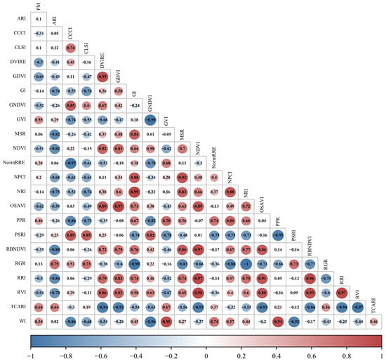
Figure 5.
Correlation analysis heatmap between spectral features and PM of rubber trees.
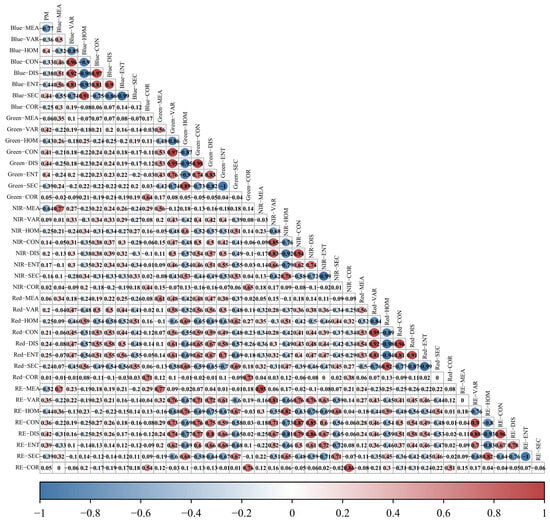
Figure 6.
Correlation analysis heatmap between textural features and PM of rubber trees.

Table 3.
Specific values and significance levels of correlation coefficients for spectral features.

Table 4.
Specific values and significance levels of correlation coefficients for texture features.
3.2. Feature Selection at Different Resolutions
3.2.1. Feature Selection Based on the SPA
The SPA was used for feature selection in four different resolution scenes, and the variation of the root mean square error (RMSE) of the SPA is shown in Figure 7. The orange line represents the 3.4 cm resolution feature set, the blue line represents the 7 cm resolution feature set, the red line represents the 14 cm resolution feature set, and the black line represents the 30 cm resolution feature set. When the resolution was 3.4 cm, 7 cm, 14 cm, and 30 cm, the number of features selected by the SPA was 14, 17, 9, and 8, respectively, and the corresponding RMSE was 0.169, 0.177, 0.233, and 0.282, respectively; thus, the RMSE increases with the increase of resolution.
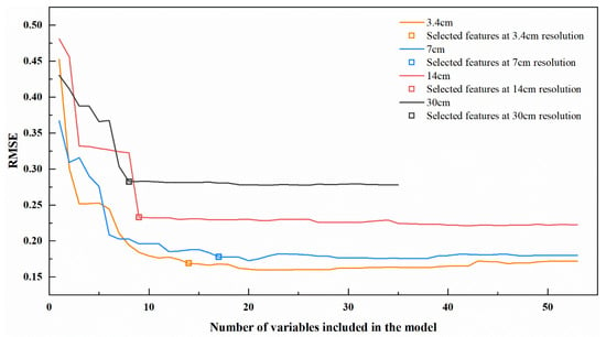
Figure 7.
RMSE plots for the number of variables selected by SPA at different resolutions.
3.2.2. Feature Selection Based on the ReliefF Algorithm
The ReliefF algorithm was used for feature selection to evaluate the importance of each feature, as shown in Figure 8. The feature variables with weights greater than 0.05 were selected as ReliefF feature subsets for datasets with spatial resolutions of 3.4 cm, 7 cm, and 14 cm, and the number of selected features was 23, 18, and 14, respectively. Meanwhile, for datasets with a resolution of 30 cm, considering that most of the features have low weight values, the weight thresholds were set individually, feature variables with weights greater than 0.03 were selected as ReliefF feature subsets, and the number of selected features was 8.
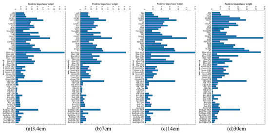
Figure 8.
Importance weight plot of the number of variables selected by ReliefF at different resolutions. (a) 3.4 cm, (b) 7 cm, (c) 14 cm, (d) 30 cm.
3.2.3. Feature Selection Based on the Boruta–SHAP Algorithm
The Boruta–SHAP algorithm was used for feature selection, as shown in Figure 9. These features were ranked in order of importance from top to bottom, where green features were selected, blue features were “shadow features”, and red features were removed. When the resolution was 3.4 cm, 7 cm, 14 cm, and 30 cm, the number of features selected by Boruta–SHAP was 44, 43, 40, and 34, respectively, and 18, 19, 22, and 34 features were removed, respectively. The specific feature variables are shown in Table 5.
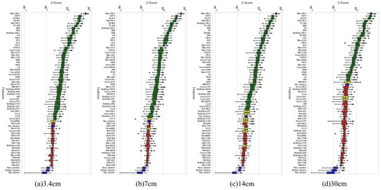
Figure 9.
Z-Score plot of the number of variables selected by Boruta–SHAP at different resolutions. (a) 3.4 cm, (b) 7 cm, (c) 14 cm, (d) 30 cm.

Table 5.
Features selected by SPA, Boruta–SHAP, and ReliefF at different resolutions.
3.3. Construction of Rubber Tree Powdery Mildew Identification Model
The feature sets selected by SPA, ReliefF, and Boruta–SHAP at different resolutions were input into KNN, SVM, and RF algorithms, respectively, to construct the rubber tree powdery mildew monitoring model, and the results of the training and validation sets are shown in Table 6 and Table 7. The accuracy of the three models in the training set is higher than that of the validation set in general. For the single model in the training set, the accuracy of KNN, SVM, and RF were 88.4~96.6%, 87.1~98.4%, and 93.7~99.5% at four different resolutions, respectively; RF showed the best classification, followed by the SVM model, while the KNN model was the worst.

Table 6.
Comparison of the classification effects of KNN, SVM, and RF models with different feature selection algorithms at different resolutions (training set).

Table 7.
Comparison of the classification effects of KNN, SVM, and RF models with different feature selection algorithms at different resolutions (validation set).
For a single model on the validation set, the classification accuracies of KNN, SVM, and RF at the four different resolutions were 73.2% to 93.3%, 79.1% to 98.2%, and 78.5% to 96.3%, respectively, and the SVM model in general had better classification than the KNN and RF classifiers. With 3.4 cm resolution, the feature set selected by the SPA had classification accuracies of 92.1%, 92.1%, and 95.7% in the KNN, SVM, and RF models, respectively, which keeps high classification accuracy on the basis of feature reduction. The feature set selected by the ReliefF algorithm had classification accuracies of 93.8%, 96.3%, and 95.7% in the KNN, SVM, and RF models, respectively, which is an improvement in overall accuracy compared to the SPA feature set. The feature set selected by the Boruta–SHAP algorithm was more robust, with classification accuracies of 95.1%, 98.2%, and 96.3% in the KNN, SVM, and RF models, respectively, with higher overall classification accuracies compared to the SPA and ReliefF algorithms. Meanwhile, with the SVM model as the benchmark, the classification accuracy of Boruta–SHAP–SVM reached 98.16%, 96.32%, 95.71%, and 88.34% at 3.4 cm, 7 cm, 14 cm, and 30 cm resolutions, respectively, and the classification accuracy was improved compared with SPA–SVM and ReliefF–SVM by 6.14%, 5.52%, 12.89%, and 9.2% and 1.84%, 0.61%, 1.23%, and 6.13%, respectively.
3.4. Rubber Tree Powdery Mildew Mapping
In this study, we used SPA, ReliefF, and Boruta–SHAP algorithms to select sensitive features as input to construct a classification model for rubber tree PM monitoring at different resolutions. From the analysis in Section 3.3, it can be seen that the SVM model with Boruta–SHAP-algorithm-selected features as input had the best overall performance at different resolutions, so the model was used for spatial distribution mapping of rubber tree PM. As shown in Figure 10, the results of PM pixel classification based on the SVM model at different resolutions (where orange indicates diseased areas and green indicates healthy areas), the rubber tree PM infection area is larger and the disease is more serious in the northwest direction of the study area. Meanwhile, comparing the recognition results, we also found that the classification results at different resolutions were basically the same. However, as the resolution decreases, the background areas such as tree branches, shadows, and canopy plants are confused with each other and result in incorrect classification. Despite this phenomenon, the constructed monitoring model for rubber tree PM identifies disease areas well at different resolutions.
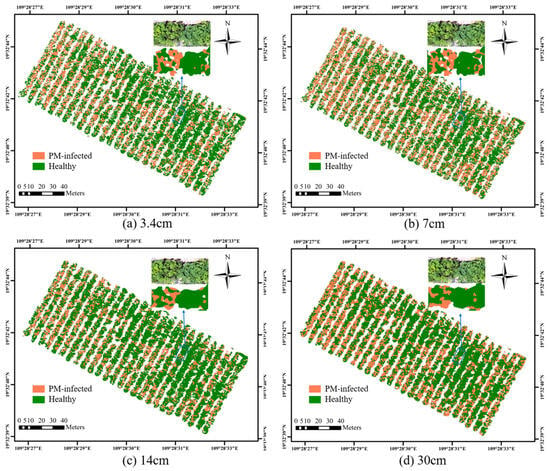
Figure 10.
Distribution and detail maps of powdery mildew of rubber trees at different resolutions. (a) 3.4 cm, (b) 7 cm, (c) 14 cm, (d) 30 cm.
4. Discussion
We found that the best monitoring accuracy was achieved for images with a spatial resolution of 3.4 cm in comparing remote sensing images with different resolutions. Meanwhile, when the images have a spatial resolution greater than 14 cm, good monitoring accuracy for rubber tree PM is achieved. The high spatial resolution of the UAV images depends on the flight altitude, but a lower flight altitude will slow down the monitoring efficiency of the UAV. For example, in the monitoring range of this study area, the flight altitude and the number of photos for acquiring 3.4 cm, 7 cm, 14 cm, and 30 cm resolutions are 60 m, 125 m, 260 m, 500 m and 208, 62, 16, and 4 photos, respectively, which indicates that choosing the appropriate flight altitude can substantially improve the efficiency of rubber tree PM identification with a certain monitoring accuracy guaranteed.
Feature selection is a critical step in model construction, and smart selection of features can reduce training time and improve accuracy [50]. To the best of our knowledge, most existing studies rely on empirical direct selection of spectral features or texture features to monitor crops [51], and these features have a large degree of redundancy. In this study, redundant features with a high correlation were removed using SPA, ReliefF, and Boruta–SHAP algorithms. For the SPA, each selected feature is related to the previous one in the process of selecting features, but the initial features are selected by random selection, so that the selected features may have more redundant information. For example, for SPA-selected features at 3.4 cm resolution in Figure 5 and Figure 6, the correlation between MSR and NPCI was 0.92, and the correlation between OSAVI and GDVI was 0.97. The ReliefF algorithm only considers feature relevance and does not analyze redundancy, and it needs to set the threshold manually for feature selection. The Boruta–SHAP algorithm enhances the explanatory ability of important features by adding SHAP values and reduces the number of features by selecting features which do not affect the performance of the model. Although the final selected features have redundancy and a higher number of features, the constructed model is more robust. Meanwhile, this study used KNN, SVM, and RF algorithms to construct models to compare the performance in four feature sets (all feature set, SPA feature set, ReliefF feature set, and Boruta–SHAP feature set) as shown in Table 7; the results show that compared with KNN and RF models, SVM models achieved 98.16%, 96.32%, 95.71%, and 88.34% of the highest classification accuracy, respectively, which also indicates that the SVM model has better generalization ability.
Although the above scheme achieved relatively well-classified results, there were misclassifications, and the misclassified samples were mostly near the soil edge and shaded ground. This may be due to the intensive planting of rubber trees; there is a large height difference between the lower canopy and the upper canopy in rubber trees, so the shading of different canopies can easily cause the mixing of healthy and shaded areas, and with the lower resolution, this phenomenon will be exacerbated. As shown in Figure 11, the gray-blue box shows the misclassification due to the mixed pixels of shade and canopy, and the orange box shows the misclassification as the resolution reduction further exacerbates the mixed pixels.

Figure 11.
Misclassification of healthy and shaded areas.
This study demonstrated that UAV-based multispectral images are well suited for rubber tree powdery mildew monitoring. Meanwhile the simulation at different scales also well achieved accuracy of detection. However, as the resolution decreases, the mixed pixel effect becomes more and more serious, leading to the decrease of monitoring accuracy. In the future, we will fly the UAV at different altitudes to acquire images with different spatial resolutions instead of simulating the image resolution. In addition, because this study used single-date multispectral images, which is a limitation in determining changes in spectral and textural parameters caused by rubber tree powdery mildew, multi-temporal monitoring of the full period of rubber tree powdery mildew development should be studied in the future. In addition, crop disease monitoring depends heavily on appropriate platforms and sensors, so in the future we will integrate other sensors (hyperspectral, thermal infrared, etc.) for remote sensing monitoring of rubber tree powdery mildew.
5. Conclusions
Rubber tree is one of the important tropical economic crops, and PM is the most damaging disease affecting the growth of rubber trees. In this study, we combined the effects of resolution (3.4 cm, 7 cm, 14 cm, 30 cm), feature selection (SPA, ReliefF, Boruta–SHAP), and classification models (KNN, SVM, RF) on monitoring PM in rubber trees. The results show that the resolution has a great influence on the identification of rubber tree PM, and the classification accuracy is high (>90%) with a spatial resolution greater than 14 cm. Compared with SPA and ReliefF algorithms, the Boruta–SHAP algorithm has better performance in optimizing feature sets with different resolutions, which reduces data dimensionality and improves data processing efficiency with a higher guarantee of high accuracy. Compared with KNN and RF models, the SVM model has a higher monitoring accuracy and generalization ability. Meanwhile, the highest overall recognition accuracy (98.16%) was achieved for rubber tree PM with the features of the Boruta–SHAP algorithm selection and the SVM model. This research provides technical support and reference for the rapid and nondestructive monitoring of rubber tree PM.
Author Contributions
Conceptualization, T.Z., J.F. and W.F.; data curation, Y.L.; formal analysis, C.Y. and W.F.; funding acquisition, W.F., J.W. and X.Z.; investigation, T.Z., C.Y. and Y.L.; methodology, T.Z. and W.F.; project administration, J.F., W.F., J.W. and X.Z.; resources, Y.L. and W.F.; software, T.Z.; supervision, W.F., H.Z., J.W. and X.Z.; validation, T.Z., J.F. and C.Y.; visualization, H.Z.; writing—original draft, T.Z.; writing—review and editing, W.F. and H.Z. All authors have read and agreed to the published version of the manuscript.
Funding
This work was supported by the National Natural Science Foundation of China (Grant No. 32160424), the Key R&D projects in Hainan Province (Grant No. ZDYF2020042), the Natural Science Foundation of Hainan Province (Grant No. 521RC1036), the Key R&D Projects in Hainan Province (Grant No. ZDYF2020195), the Academician Lan Yubin Innovation Platform of Hainan Province, the Key R&D projects in Hainan Province (Grant No. ZDYF2021GXJS036), the Innovative research projects for graduate students in Hainan Province (Grant No. Qhyb2021-11), and the Hainan Province Academician Innovation Platform (Grant No. YSPTZX202008).
Data Availability Statement
Not applicable.
Acknowledgments
We would like to thank the reviewers for their valuable suggestions on this manuscript.
Conflicts of Interest
The authors declare no conflict of interest.
Appendix A

Table A1.
The specific parameters of the three classification methods.
Table A1.
The specific parameters of the three classification methods.
| Type | KNN | SVM | RF |
|---|---|---|---|
| All feature | |||
| 3.4 cm | leaf_size = 10, n_neighbors = 9, P = 1, weights = ‘uniform’ | C = 147, gamma = 1/62, kernel = ‘rbf’ | max_depth = 10, n_estimators = 400 |
| 7 cm | leaf_size = 10, n_neighbors = 13, P = 1, weights = ‘distance’ | C = 186, gamma = 1/62, kernel = ‘rbf’ | max_depth = 10, n_estimators = 400 |
| 14 cm | leaf_size = 10, n_neighbors = 7, P = 1, weights = ‘distance’ | C = 182, gamma = 1/62, kernel = ‘rbf’ | max_depth = 10, n_estimators = 400 |
| 30 cm | leaf_size = 10, n_neighbors = 15, P = 1, weights = ‘distance’ | C = 187, gamma = 1/62, kernel = ‘rbf’ | max_depth = 14, n_estimators = 1000 |
| SPA | |||
| 3.4 cm | leaf_size = 10, n_neighbors = 5, P = 1, weights = ‘distance’ | C = 177, gamma = 1/14, kernel = ‘rbf’ | max_depth = 14, n_estimators = 600 |
| 7 cm | leaf_size = 10, n_neighbors = 13, P = 1, weights = ‘distance’ | C = 188, gamma = 1/17, kernel = ‘rbf’ | max_depth = 8, n_estimators = 1000 |
| 14 cm | leaf_size = 10, n_neighbors = 7, P = 1, weights = ‘distance’ | C = 197, gamma = 1/9, kernel = ‘rbf’ | max_depth = 6, n_estimators = 600 |
| 30 cm | leaf_size = 10, n_neighbors = 11, P = 1, weights = ‘distance’ | C = 131, gamma = 1/8, kernel = ‘rbf’ | max_depth = 14, n_estimators= 1000 |
| ReliefF | |||
| 3.4 cm | leaf_size = 10, n_neighbors = 5, P = 1, weights = ‘distance’ | C = 185, gamma = 1/23, kernel = ‘rbf’ | max_depth = 8, n_estimators = 400 |
| 7 cm | leaf_size = 10, n_neighbors = 5, P = 1, weights = ‘uniform’ | C = 179, gamma = 1/18, kernel = ‘rbf’ | max_depth = 14, n_estimators = 400 |
| 14 cm | leaf_size = 10, n_neighbors = 5, P = 1, weights = ‘uniform’ | C = 194, gamma = 1/14, kernel = ‘rbf’ | max_depth = 8, n_estimators = 600 |
| 30 cm | leaf_size = 10, n_neighbors = 5, P = 1, weights = ‘distance’ | C = 112, gamma = 1/8, kernel = ‘rbf’ | max_depth = 10, n_estimators = 400 |
| Boruta–SHAP | |||
| 3.4 cm | leaf_size = 10, n_neighbors = 5, P = 1, weights = ‘uniform’ | C = 105, gamma = 1/44, kernel = ‘rbf’ | max_depth = 12, n_estimators = 1000 |
| 7 cm | leaf_size = 10, n_neighbors = 11, P = 1, weights = ‘distance’ | C = 127, gamma = 1/43, kernel = ‘rbf’ | max_depth = 12, n_estimators = 400 |
| 14 cm | leaf_size = 10, n_neighbors = 9, P = 1, weights = ‘uniform’ | C = 162, gamma = 1/40, kernel = ‘rbf’ | max_depth = 12, n_estimators = 800 |
| 30 cm | leaf_size = 10, n_neighbors = 11, P = 2, weights = ‘distance’ | C = 199, gamma = 1/28, kernel = ‘rbf’ | max_depth = 8, n_estimators = 400 |
References
- Singh, A.K.; Liu, W.; Zakari, S.; Wu, J.; Yang, B.; Jiang, X.J.; Zhu, X.; Zou, X.; Zhang, W.; Chen, C.; et al. A Global Review of Rubber Plantations: Impacts on Ecosystem Functions, Mitigations, Future Directions, and Policies for Sustainable Cultivation. Sci. Total Environ. 2021, 796, 148948. [Google Scholar] [CrossRef]
- Bai, R.; Wang, J.; Li, N. Climate Change Increases the Suitable Area and Suitability Degree of Rubber Tree Powdery Mildew in China. Ind. Crops Prod. 2022, 189, 115888. [Google Scholar] [CrossRef]
- Liyanage, K.K.; Khan, S.; Mortimer, P.E.; Hyde, K.D.; Xu, J.; Brooks, S.; Ming, Z. Powdery Mildew Disease of Rubber Tree. For. Pathol. 2016, 46, 90–103. [Google Scholar] [CrossRef]
- Qin, B.; Zheng, F.; Zhang, Y. Molecular Cloning and Characterization of a Mlo Gene in Rubber Tree (Hevea brasiliensis). J. Plant Physiol. 2015, 175, 78–85. [Google Scholar] [CrossRef]
- Cao, X.; Xu, X.; Che, H.; West, J.S.; Luo, D. Effects of Temperature and Leaf Age on Conidial Germination and Disease Development of Powdery Mildew on Rubber Tree. Plant Pathol. 2021, 70, 484–491. [Google Scholar] [CrossRef]
- Zhai, D.-L.; Thaler, P.; Luo, Y.; Xu, J. The Powdery Mildew Disease of Rubber (Oidium heveae) Is Jointly Controlled by the Winter Temperature and Host Phenology. Int. J. Biometeorol. 2021, 65, 1707–1718. [Google Scholar] [CrossRef]
- Li, X.; Bi, Z.; Di, R.; Liang, P.; He, Q.; Liu, W.; Miao, W.; Zheng, F. Identification of Powdery Mildew Responsive Genes in Hevea Brasiliensis through MRNA Differential Display. Int. J. Mol. Sci. 2016, 17, 181. [Google Scholar] [CrossRef]
- Azizan, F.A.; Kiloes, A.M.; Astuti, I.S.; Abdul Aziz, A. Application of Optical Remote Sensing in Rubber Plantations: A Systematic Review. Remote Sens. 2021, 13, 429. [Google Scholar] [CrossRef]
- Santoso, H.; Gunawan, T.; Jatmiko, R.H.; Darmosarkoro, W.; Minasny, B. Mapping and Identifying Basal Stem Rot Disease in Oil Palms in North Sumatra with QuickBird Imagery. Precis. Agric. 2011, 12, 233–248. [Google Scholar] [CrossRef]
- Zhang, B.; Ye, H.; Lu, W.; Huang, W.; Wu, B.; Hao, Z.; Sun, H. A Spatiotemporal Change Detection Method for Monitoring Pine Wilt Disease in a Complex Landscape Using High-Resolution Remote Sensing Imagery. Remote Sens. 2021, 13, 2083. [Google Scholar] [CrossRef]
- Shafi, U.; Mumtaz, R.; García-Nieto, J.; Hassan, S.A.; Zaidi, S.A.R.; Iqbal, N. Precision Agriculture Techniques and Practices: From Considerations to Applications. Sensors 2019, 19, 3796. [Google Scholar] [CrossRef]
- Pádua, L.; Marques, P.; Martins, L.; Sousa, A.; Peres, E.; Sousa, J.J. Monitoring of Chestnut Trees Using Machine Learning Techniques Applied to UAV-Based Multispectral Data. Remote Sens. 2020, 12, 3032. [Google Scholar] [CrossRef]
- Yang, W.; Xu, W.; Wu, C.; Zhu, B.; Chen, P.; Zhang, L.; Lan, Y. Cotton Hail Disaster Classification Based on Drone Multispectral Images at the Flowering and Boll Stage. Comput. Electron. Agric. 2021, 180, 105866. [Google Scholar] [CrossRef]
- Guo, A.; Huang, W.; Dong, Y.; Ye, H.; Ma, H.; Liu, B.; Wu, W.; Ren, Y.; Ruan, C.; Geng, Y. Wheat Yellow Rust Detection Using UAV-Based Hyperspectral Technology. Remote Sens. 2021, 13, 123. [Google Scholar] [CrossRef]
- Ye, H.; Huang, W.; Huang, S.; Cui, B.; Dong, Y.; Guo, A.; Ren, Y.; Jin, Y. Recognition of Banana Fusarium Wilt Based on UAV Remote Sensing. Remote Sens. 2020, 12, 938. [Google Scholar] [CrossRef]
- Wei, Y.; Yang, T.; Ding, X.; Gao, Y.; Yuan, X.; He, L.; Wang, Y.; Duan, J.; Feng, W. Wheat lodging region identification based on unmanned aerial vehicle multispectral imagery with different spatial resolutions. Smart Agric. 2023, 5, 56–67. [Google Scholar]
- Zhao, J.; Jin, Y.; Ye, H.; Huang, W.; Dong, Y.; Fan, L.; Ma, H.; Jiang, J. Remote Sensing Monitoring of Areca Yellow Leaf Disease Based on UAV Multi-Spectral Images. Trans. Chin. Soc. Agric. Eng. 2020, 36, 54–61. [Google Scholar]
- Ma, L.; Huang, X.; Hai, Q.; Gang, B.; Tong, S.; Bao, Y.; Dashzebeg, G.; Nanzad, T.; Dorjsuren, A.; Enkhnasan, D. Model-Based Identification of Larix Sibirica Ledeb. Damage Caused by Erannis Jacobsoni Djak. Based on UAV Multispectral Features and Machine Learning. Forests 2022, 13, 2104. [Google Scholar] [CrossRef]
- Narmilan, A.; Gonzalez, F.; Salgadoe, A.S.A.; Powell, K. Detection of White Leaf Disease in Sugarcane Using Machine Learning Techniques over UAV Multispectral Images. Drones 2022, 6, 230. [Google Scholar] [CrossRef]
- Rodriguez, J.; Lizarazo, I.; Prieto, F.; Angulo-Morales, V. Assessment of Potato Late Blight from UAV-Based Multispectral Imagery. Comput. Electron. Agric. 2021, 184, 106061. [Google Scholar] [CrossRef]
- Mei, S.; Hou, S.; Cui, H.; Feng, F.; Rong, W. Characterization of the Interaction between Oidium Heveae and Arabidopsis Thaliana. Mol. Plant Pathol. 2016, 17, 1331–1343. [Google Scholar] [CrossRef]
- Di Gennaro, S.F.; Toscano, P.; Gatti, M.; Poni, S.; Berton, A.; Matese, A. Spectral Comparison of UAV-Based Hyper and Multispectral Cameras for Precision Viticulture. Remote Sens. 2022, 14, 449. [Google Scholar] [CrossRef]
- Borra-Serrano, I.; Peña, J.M.; Torres-Sánchez, J.; Mesas-Carrascosa, F.J.; López-Granados, F. Spatial Quality Evaluation of Resampled Unmanned Aerial Vehicle-Imagery for Weed Mapping. Sensors 2015, 15, 19688–19708. [Google Scholar] [CrossRef]
- Garcia-Ruiz, F.; Sankaran, S.; Maja, J.M.; Lee, W.S.; Rasmussen, J.; Ehsani, R. Comparison of Two Aerial Imaging Platforms for Identification of Huanglongbing-Infected Citrus Trees. Comput. Electron. Agric. 2013, 91, 106–115. [Google Scholar] [CrossRef]
- Wang, L.-F.; Wang, M.; Zhang, Y. Effects of Powdery Mildew Infection on Chloroplast and Mitochondrial Functions in Rubber Tree. Trop. Plant Pathol. 2014, 39, 242–250. [Google Scholar] [CrossRef]
- Liang, Y.; Kou, W.; Lai, H.; Wang, J.; Wang, Q.; Xu, W.; Wang, H.; Lu, N. Improved Estimation of Aboveground Biomass in Rubber Plantations by Fusing Spectral and Textural Information from UAV-Based RGB Imagery. Ecol. Indic. 2022, 142, 109286. [Google Scholar] [CrossRef]
- Gitelson, A.A.; Kaufman, Y.J.; Stark, R.; Rundquist, D. Novel Algorithms for Remote Estimation of Vegetation Fraction. Remote Sens. Environ. 2002, 80, 76–87. [Google Scholar] [CrossRef]
- Zhou, J.; Yungbluth, D.; Vong, C.N.; Scaboo, A.; Zhou, J. Estimation of the Maturity Date of Soybean Breeding Lines Using UAV-Based Multispectral Imagery. Remote Sens. 2019, 11, 2075. [Google Scholar] [CrossRef]
- Patrick, A.; Pelham, S.; Culbreath, A.; Holbrook, C.C.; De Godoy, I.J.; Li, C. High Throughput Phenotyping of Tomato Spot Wilt Disease in Peanuts Using Unmanned Aerial Systems and Multispectral Imaging. IEEE Instrum. Meas. Mag. 2017, 20, 4–12. [Google Scholar] [CrossRef]
- Zarco-Tejada, P.J.; Berjón, A.; Lopez-Lozano, R.; Miller, J.R.; Martín, P.; Cachorro, V.; González, M.R.; De Frutos, A. Assessing Vineyard Condition with Hyperspectral Indices: Leaf and Canopy Reflectance Simulation in a Row-Structured Discontinuous Canopy. Remote Sens. Environ. 2005, 99, 271–287. [Google Scholar] [CrossRef]
- Chandel, A.K.; Khot, L.R.; Sallato, B. Apple Powdery Mildew Infestation Detection and Mapping Using High-Resolution Visible and Multispectral Aerial Imaging Technique. Sci. Hortic. 2021, 287, 110228. [Google Scholar] [CrossRef]
- Rouse, J.W. Monitoring the Vernal Advancement of Retrogradation of Natural Vegetation; Type III, Final Report; NASA/GSFC: Greenbelt, MD, USA, 1974; Volume 371.
- Filella, I.; Serrano, L.; Serra, J.; Penuelas, J. Evaluating Wheat Nitrogen Status with Canopy Reflectance Indices and Discriminant Analysis. Crop Sci. 1995, 35, 1400–1405. [Google Scholar] [CrossRef]
- Wang, Z.J.; Wang, J.H.; Liu, L.Y.; Huang, W.J.; Zhao, C.J.; Wang, C.Z. Prediction of Grain Protein Content in Winter Wheat (Triticum Aestivum L.) Using Plant Pigment Ratio (PPR). Field Crops Res. 2004, 90, 311–321. [Google Scholar] [CrossRef]
- Merzlyak, M.N.; Gitelson, A.A.; Chivkunova, O.B.; Rakitin, V.Y.U. Non-destructive Optical Detection of Pigment Changes during Leaf Senescence and Fruit Ripening. Physiol. Plant. 1999, 106, 135–141. [Google Scholar] [CrossRef]
- Wang, F.-M.; Huang, J.-F.; Tang, Y.-L.; Wang, X.-Z. New Vegetation Index and Its Application in Estimating Leaf Area Index of Rice. Rice Sci. 2007, 14, 195–203. [Google Scholar] [CrossRef]
- Zheng, H.; Cheng, T.; Zhou, M.; Li, D.; Yao, X.; Tian, Y.; Cao, W.; Zhu, Y. Improved Estimation of Rice Aboveground Biomass Combining Textural and Spectral Analysis of UAV Imagery. Precis. Agric. 2019, 20, 611–629. [Google Scholar] [CrossRef]
- Xue, L.; Cao, W.; Luo, W.; Dai, T.; Zhu, Y. Monitoring Leaf Nitrogen Status in Rice with Canopy Spectral Reflectance. Agron. J. 2004, 96, 135–142. [Google Scholar] [CrossRef]
- Haboudane, D.; Miller, J.R.; Tremblay, N.; Zarco-Tejada, P.J.; Dextraze, L. Integrated Narrow-Band Vegetation Indices for Prediction of Crop Chlorophyll Content for Application to Precision Agriculture. Remote Sens. Environ. 2002, 81, 416–426. [Google Scholar] [CrossRef]
- Woebbecke, D.M.; Meyer, G.E.; Von Bargen, K.; Mortensen, D.A. Color Indices for Weed Identification under Various Soil, Residue, and Lighting Conditions. Trans. ASAE 1995, 38, 259–269. [Google Scholar] [CrossRef]
- YIN, Y.; WANG, G. Hyperspectral Characteristic Wavelength Selection Method for Moldy Maize Based on Continuous Projection Algorithm Fusion Information Entropy. J. Nucl. Agric. Sci. 2020, 34, 356–362. [Google Scholar]
- Wang, Z.; Zhang, Y.; Chen, Z.; Yang, H.; Sun, Y.; Kang, J.; Yang, Y.; Liang, X. Application of ReliefF Algorithm to Selecting Feature Sets for Classification of High Resolution Remote Sensing Image. In Proceedings of the 2016 IEEE International Geoscience and Remote Sensing Symposium (IGARSS), Beijing, China, 10–15 July 2016; pp. 755–758. [Google Scholar]
- Akbar, S.; Ali, F.; Hayat, M.; Ahmad, A.; Khan, S.; Gul, S. Prediction of Antiviral Peptides Using Transform Evolutionary & SHAP Analysis Based Descriptors by Incorporation with Ensemble Learning Strategy. Chemom. Intell. Lab. Syst. 2022, 230, 104682. [Google Scholar]
- Islam, N.; Rashid, M.M.; Wibowo, S.; Xu, C.-Y.; Morshed, A.; Wasimi, S.A.; Moore, S.; Rahman, S.M. Early Weed Detection Using Image Processing and Machine Learning Techniques in an Australian Chilli Farm. Agriculture 2021, 11, 387. [Google Scholar] [CrossRef]
- Oide, A.H.; Nagasaka, Y.; Tanaka, K. Performance of Machine Learning Algorithms for Detecting Pine Wilt Disease Infection Using Visible Color Imagery by UAV Remote Sensing. Remote Sens. Appl. Soc. Environ. 2022, 28, 100869. [Google Scholar] [CrossRef]
- Ong, P.; Teo, K.S.; Sia, C.K. UAV-Based Weed Detection in Chinese Cabbage Using Deep Learning. Smart Agric. Technol. 2023, 4, 100181. [Google Scholar] [CrossRef]
- Xu, P.; Fu, L.; Xu, K.; Sun, W.; Tan, Q.; Zhang, Y.; Zha, X.; Yang, R. Investigation into Maize Seed Disease Identification Based on Deep Learning and Multi-Source Spectral Information Fusion Techniques. J. Food Compos. Anal. 2023, 119, 105254. [Google Scholar] [CrossRef]
- Zhang, H.; Huang, L.; Huang, W.; Dong, Y.; Weng, S.; Zhao, J.; Ma, H.; Liu, L. Detection of Wheat Fusarium Head Blight Using UAV-Based Spectral and Image Feature Fusion. Front. Plant Sci. 2022, 13, 1004427. [Google Scholar] [CrossRef]
- DadrasJavan, F.; Samadzadegan, F.; Seyed Pourazar, S.H.; Fazeli, H. UAV-Based Multispectral Imagery for Fast Citrus Greening Detection. J. Plant Dis. Prot. 2019, 126, 307–318. [Google Scholar] [CrossRef]
- Venkatesh, B.; Anuradha, J. A Review of Feature Selection and Its Methods. Cybern. Inf. Technol. 2019, 19, 3–26. [Google Scholar] [CrossRef]
- Torresan, C.; Berton, A.; Carotenuto, F.; Di Gennaro, S.F.; Gioli, B.; Matese, A.; Miglietta, F.; Vagnoli, C.; Zaldei, A.; Wallace, L. Forestry Applications of UAVs in Europe: A Review. Int. J. Remote Sens. 2017, 38, 2427–2447. [Google Scholar] [CrossRef]
Disclaimer/Publisher’s Note: The statements, opinions and data contained in all publications are solely those of the individual author(s) and contributor(s) and not of MDPI and/or the editor(s). MDPI and/or the editor(s) disclaim responsibility for any injury to people or property resulting from any ideas, methods, instructions or products referred to in the content. |
© 2023 by the authors. Licensee MDPI, Basel, Switzerland. This article is an open access article distributed under the terms and conditions of the Creative Commons Attribution (CC BY) license (https://creativecommons.org/licenses/by/4.0/).