Abstract
The aerial flexible-joint robot (AFJR) manipulation system has been widely used in recent years. To handle uncertainty, the input saturation and the output constraint existing in the system, a fixed-time observer-based adaptive control scheme (FTOAC) is proposed. First, to estimate the input saturation and disturbances from the internal force between the robot and the flight platform, a fixed-time observer is designed. Second, a tangent-barrier Lyapunov function is introduced to implement the output constraint. Third, adaptive neural networks are introduced for the online identification of nonlinear unknown dynamics in the system. In addition, a fixed-time compensator is designed in this paper to eliminate the adverse effects caused by filtering errors. The stability analysis shows that all the signals of the closed-loop system are bounded, and the system satisfies the condition of fixed-time convergence. Finally, the simulation results prove the superiority of the proposed control strategy by comparing it with the previous schemes.
1. Introduction
In recent years, the application of unmanned aerial vehicles (UAVs) has been extended to active missions by equipping them with robotic arms [1,2], such as picking up and transporting important materials or reaching hard-to-reach places for emergency repairs [3]. Due to the advantages of being lightweight and having high mobility and low energy consumption, robotic arms with flexible joints (FJRs) are suitable for application in UAVs [4]. The dynamics model of the aerial flexible-joint robot (AFJR) is a highly coupled system, which is composed of both the UAV and a robotic manipulator [5]. The AFJR usually works in a hovering state when grasping a target. Therefore, the challenging work for the control of the AFJR is to achieve accurate-fast control for the FJR subsystem. At this moment, the coupling effect of the UAV to manipulation is treated as a disturbance. Moreover, the nonlinear unknown dynamics of FJR systems [6,7], output constraints, and input saturation [8,9] are inevitable in actual applications. Therefore, it is valuable to study the tracking control of the AFJR by considering these issues.
Nonlinear system control approaches are broadly classified as asymptotic stabilization control and finite-time control. The system with asymptotic stability control has an infinite stabilization time. In addition, finite-time control can realize system stabilization in a bounded time. Many researchers have investigated finite-time control for FJR systems recently [10,11]. The finite-time strategy, on the other hand, determines the stability time based on the initial conditions. To circumvent this limitation, fixed-time control is proposed, which allows the system to converge to equilibrium in a finite time regardless of the initial conditions. Because of this trait, fixed-time stability is more suitable for engineering applications. In [12], an adaptive fuzzy event-triggered fixed-time real-tracking control method was proposed for FJR systems. S. Binazadeh et al. [13] designed a fixed-time super-torsional sliding mode tracking strategy for nonlinear networked FJRs.
In terms of dealing with unknown dynamics in nonlinear systems, neural network-based control is an effective solution. In [14], an adaptive neural control method for electrically driven FJRs was studied, applying radial basis function neural networks (RBFNNs) to approximate the unknown nonlinearity of the system. In [15], an adaptive neural network control based on integral Lyapunov functions was proposed for task tracking under the uncertainty of the FJR. In [16], nonlinear functions were approximated by using neural networks (NN). The authors of [17] proposed an observer-based RBFNN to estimate the state variables of a normal system. Most of the above NN-based schemes were carried out in the backstepping framework. However, the computing explosion problem is unavoidable for repeated differentiation of virtual control. To solve this issue, a command filtering method was used in [18,19,20]. To eliminate the effect of filtering errors, instruction filtering compensation strategies were proposed in [21,22]. Inspired by the above analysis, this paper intends to investigate fixed-time stable neural network control schemes to solve the fast-stability problem of FJR systems when considering the complexity explosion problem and filtering disturbances.
In the above-mentioned works, disturbances were not considered, such as the internal force between the arm and the drone, and input saturation. The performance and stability of the AFJR would significantly degrade [23,24]. Therefore, an AFJR should be able to tolerate unknown disturbances. The commonly used anti-saturation methods are function approximation and auxiliary system compensation. The saturation function approximation methods employ the mean value theorem to handle the unknown function, but the approximation error cannot be avoided [25,26]. On the contrary, via the auxiliary system approaches, the errors between the nominal and saturated inputs are treated as disturbances. By introducing an observer to estimate the disturbances and designing a compensated controller, the input saturation can be handled precisely to make the system out of the saturation region [27,28,29]. For example, the tracking control of a multi-link FJR system with input saturation was studied in [30], where an auxiliary dynamic system was used to handle the input saturation. In [31], two auxiliary systems were introduced to handle the input saturation of a free-flying FJR. A nonlinear perturbation observer was proposed in [32] for handling the input saturation of the FJR. By disturbance observer techniques, the disturbances of the aerial manipulation system can be addressed [33,34]. As a result, combining the fixed-time stability theory and the observer technique to deal with input saturation and model coupling disturbances in the AFJR is worth investigating.
Furthermore, in some practical areas of work, the outputs of robotic systems are subject to special constraints, which receive attention from scholars. In [35], the tangent-type barrier Lyapunov function was used for the system with output constraints. By designing error bounds, the unknown Euler–Lagrange system satisfies the prescribed tracking accuracy and output constraints [36]. For unconstrained feedback nonlinear systems with asymmetric and time-varying output constraints, the barrier Lyapunov function (BLF) and error transformation techniques was used [37]. The tangent-type barrier Lyapunov function was used in [38] to handle the state constraints of the FJR. In [39], the output constraint of RMFJ was implemented to improve the safety of the robot. The authors of [40] proposed an instruction filter-based backstepping control method for trajectory tracking control of FJR with full state constraints. Although the above studies successfully addressed the effect of saturation nonlinearity and output constraints, it is still worth further research on how to deal with the fixed-time stability of FJR systems with the input saturation and output constraint.
Inspired by the above analysis, a fixed-time observer-based adaptive tracking control scheme (FTOAC) is proposed for the Aerial FJR with an input saturation and output constraint, where the main contributions are:
- Unlike the works of [14,41], which requires the approximation of each subfunction of the nonlinear function sets, this paper cleverly converts the unknown set of nonlinear functions present in the n-link FJR system into the forms of the norm, so that the whole controller needs only two neural networks and one adaptive law, thus saving computational resources.
- Through the dynamic surface technique, a command filter is introduced to avoid the “complexity explosion” problem during backstepping design, and a fixed-time compensator is designed to handle the influences of the filtering errors.
- Different from [42], the input saturation and output constraint are solved simultaneously via the proposed FTOAC scheme, where a fixed-time observer is designed to estimate the input saturation and disturbances existing in the AFJR, and the tangent-type Lyapunov barrier function is constructed to realize the constraint out of the system.
2. Problem Statement and Preliminaries
2.1. Problem Statement
The AFJR system can be seen in Figure 1. The system can be decoupled as the FJR subsystem and UAV subsystem. The AFJR usually works in a hovering state when grasping a target. Therefore, the main control task of the AFJR is to achieve accurate-fast control for the FJR subsystem, and the interactions generated by the UAV platform are treated as disturbances [43]. In combination with [24], the dynamic model of the n-link FJR can be written as
where the interpretations of the symbols therein are shown in Table 1.
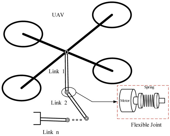
Figure 1.
Structure of Aerial FJR.

Table 1.
The symbols of the FJR system.
Moreover, the input voltage range of the motor is limited to certain specific voltages in practice, i.e., the motor saturation limit [44]. Thus, it is inevitable that the actuator is subject to input saturation. The i-th control input with saturation nonlinearity can be expressed as
where indicates the saturation value of the control input. In addition, the FJR system needs to consider obstacles in the motion space when performing the task, so the output is often constrained. In introducing the variables , the system with input saturation and output constraint can be represented as
where , and the output is constrained in the following compact set
This paper aims to suggest a fixed-time tracking scheme for the FJR system so that the output can follow the desired trajectory , all the signals in the system are bounded, the output constraint requirements are not violated, and the input saturation can be overcome.
2.2. Preliminaries
To achieve fixed-time tracking control for the Aerial FJR system existing unknown continuous functions, input saturations, and out constraints, the following definitions, assumptions, and lemmas are given.
Assumption 1
[38]. The reference trajectory satisfies with , and its n-th order time derivatives are continuously bounded.
Assumption 2.
The disturbancesof the AFJR are bounded with , where are positive constants .
Remark 1.
Assumption 1 is the basic requirement of the backstepping control method. Assumption 2 provides that the internal disturbances from the drone are bounded, which is a basic prerequisite for the stability of the whole control system.
Definition 1
[45]. Considering a smooth-nonlinear dynamic system , assume that the system is stable at the origin. If holds for all , in which is a finite time constant, the system is stable in a finite-time interval. If the time constant has an upper bound, the system is fixed-time stable.
Lemma 1.
[46]. For a positive definite function , if there exists , , and , such that
Then, the nonlinear system is globally practical fixed-time stable, and the converging time satisfies
Remark 2.
Definition 1 provides the definition of the fixed-time stability system. Lemma 1 shows how to design the Lyapunov function for a fixed-time controller. To achieve the fixed-time control, the AFJR system should satisfy the conditions of Definition 1 and Lemma 1.
Lemma 2.
[47]. For real variables ,, if are positive constants, the relationship holds
Lemma 3.
[48]. Let and , then
Lemma 4.
[49]. If an unknown continuous function is defined on a compact , can be approximated by the RBFNN
Define , where are the vectors of the i-th neural network.
Remark 3.
Due to the existence of unknown parameters and unknown kinetic functions within the system, the controller cannot be designed directly. With the help of Lemma 4, RBFNNs are used to estimate the unknown dynamics of the system.
3. The Design of FTOAC
Combining DSC, backstepping techniques, and neural networks, the FTOAC is designed in this section.
3.1. The Fixed-Time Observer
Unlike the approximated method of [42], we try to compensate for the disturbance, where the i-th disturbance is defined as
Thus, the model of n-link FJR can be rewritten as
where .
Design the observer as
where
Theorem 1.
Consider the saturation system described by(13), and assume that the term satisfies , where is a known constant. Define and as the states of the designed fixed-time observers. Then, the terms can be estimated within a fixed time through and .
The proof of Theorem 1 is presented in Appendix A.
3.2. The Dynamic Surfaces
To overcome the problem of “complex explosion”, the first-order filter is introduced as
in which is a positive designed constant, represents the input vector, and denotes the output vector.
Then, a compensated mechanism as follows is designed to eliminate the filtering errors.
where are positive constants and are the filter errors
Remark 4.
The backstepping design needs to directly derive the virtual control law. Because the virtual control law of a nonlinear system is complex, the derivation is sometimes infeasible. By introducing the filter, the derivation of the virtual control law can be avoided. However, filter errors have some impact on the system performance. Given this, this paper considers a filter compensation mechanism convergence to eliminate the filtering error while meeting the fixed-time stability requirements.
Therefore, the dynamic surfaces are given as
3.3. The Design Process of the Backstepping Controller
Step 1: To achieve the output constraint, the Lyapunov barrier function [38] is adopted as
where , .
By defining the function , the derivative of can be obtained as
Importing (17) into (21) results in
Construct the virtual control law as
where are positive design constants.
Taking the first equation of (17), and (23) into (21) generates
Step 2: According to (19), we have
Taking the second equation of (13) and (17) into (25) results in
According to (18) and (19), we know that . Thus, (26) can be rewritten as
Choose the Lyapunov function as
where , is the estimation of , and is a positive constant.
Taking the derivative of leads to
where
Based on Lemma 4, a neural network system can be used to approximate the unknown function . For any given , we have
where , and . Through Young’s inequality, one obtains
where is a positive design parameter.
By inserting(31) and (32) into (29), one obtains
Design the virtual control law as
where .
Taking (34) into (33) generates
Step 3: Choose the candidate Lyapunov function as
Taking its derivative leads to
Based on (19), we have
Substituting (13) (17) into the equation (38) generates
By combining (19) with (18), we have
Accordingly, (37) can be rewritten as
By Young’s inequality, Bringing (35) into (41) results in
Construct the virtual control law as
where .
Therefore, one obtains
Step 4: Because , we have
According to (13) and (14), we have
The candidate Lyapunov function is constructed as
Taking the derivative for results in
According to (46), we have
where the functions are defined as
Based on Lemma 4, can be approximated as
with the estimated error . By performing the same with (31), we have
Then, becomes
Design the actual controller as
Inserting (54) into (53) leads to
Design the adaptive law as
By combining with (56), we have
According to Lemma 2 and Lemma 3, one obtains
Step 5: Choose the Lyapunov function as
According to (17), we have
Then,
where .
Similar to [39], can be obtained in a limited time with .
With the help of Young’s inequality, one obtains
where .
Bringing (62) into (61) yields
in which .
3.4. Stability Analysis
Theorem 2.
For the FJR (13) with the input saturation (2) and the output-constrained condition (4), by introducing the actual controller (54) in conjunction with the virtual control laws (23), (34), (43) and the adaptive law (56), all signals of the closed-loop control system are bounded, the system can track the reference signals within the fixed-time .
Proof.
Construct the whole Lyapunov function as
By combining (58) with (63), we have
in which .
The inequation (65) can be rewritten as
where According to Lemma 1, by choosing the appropriate parameters, the tracking errors can be limited to a small residual set within a fixed-time interval. The proof of Theorem 2 has been finished. The overall control scheme is shown in Figure 2.
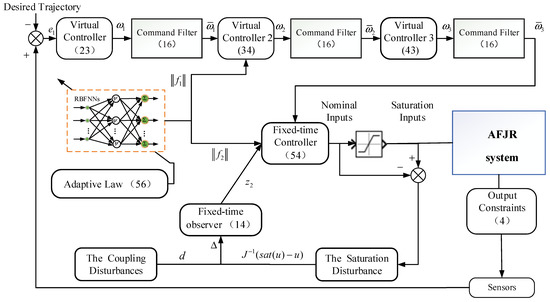
Figure 2.
System control structure diagram.
The sensors are used to detect the output signal of the AFJR. The tracking error can be obtained by comparing the output signal with the desired trajectory. Then, by introducing the command filter and the compensation mechanism, dynamic surfaces are designed. Based on the dynamic surface technique, the backstepping technique, and the fixed-time stability theory, the virtual controllers and the actual fixed-time controller are constructed in turn, in which the RBFNNs and the adaptive law are used to approximate the unknown function in the system. A fixed-time observer is introduced to estimate the disturbances .
4. Simulation
This section introduces a series of simulation examples to demonstrate the effectiveness of the presented control scheme in this paper. The simulations are carried out in MATLAB R2021a/Simulink. A two-link FJR is chosen as the object and its dynamics are described by Equation (1) with
where
As referred to in the literature [10], the parameters of the two-link FJR are listed in Table 2. The initial values of the system are chosen as and are the desired trajectories of joint 1 and joint 2, respectively. Then, select the constants of the control system as The designed parameters of filters 1, 2, and 3 are selected as , respectively. The parameters of the compensated mechanism are . The RBFNNs of this paper include 11 nodes, and the center and width of the Gaussian functions are chosen respectively as and
Table 2.
The parameters of the two-link FJR system.
4.1. The FTOAC under Filtering Compensation and Saturations
To analyze the effects of the filter compensation and different input saturation values on the control performance, four cases with different control parameters are chosen for comparison, as follows:
Case 1: The system works without the filter compensation (17), where the controller parameters are set as .
Case 2: The system works by the proposed FTOAC, where the controller parameters are set as
Case 3: The system works by the proposed FTOAC, where the controller parameters are set as
Case 4: The system works by the proposed FTOAC, where the controller parameters are set as
Case 1 represents the control scheme without the filter compensation. Cases 2, 3, and 4 represent the fixed-time stabilization control strategy with the filter compensation. The simulation results are shown in Figure 3, Figure 4, Figure 5 and Figure 6. Figure 3 and Figure 4 reveal the tracking performance. It can be seen that the system outputs can track the desired trajectory well using the proposed composite controller, and the tracking errors of both joints of the FJR are kept within a small range. In contrast, there is a lot of volatility in the tracking errors in Case 1. In comparing the tracking trajectories and error trajectories of Cases 2, 3, and 4, we know that the FJR system still has good tracking performance. However, the smaller the saturation value , the greater the vibration of the system.
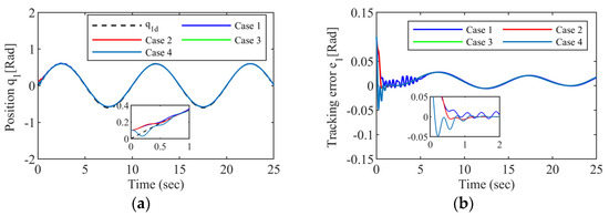
Figure 3.
Tracking performance of joint 1: (a) Tracking trajectory; (b) Tracking error.
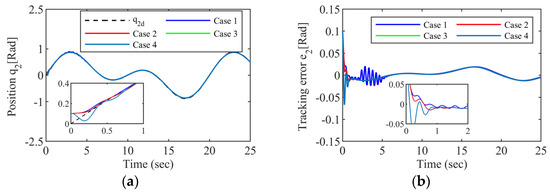
Figure 4.
Tracking performance of joint 2: (a) Tracking trajectory; (b) Tracking error.
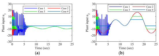
Figure 5.
The actual control input: (a) Joint 1; (b) Joint 2.
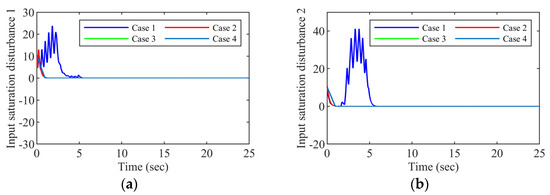
Figure 6.
The estimation of the input saturation: (a) Joint 1; (b) Joint 2.
In order to prove the correctness of the proposed method, we introduce the Mean Value (MV) and Root Mean Square (RMS) to evaluate the tracking error.
The quantities of the tracking errors are presented in Table 3. We know that Case 2 has the smallest MV and RMS.
Table 3.
Quantity table of tracking error.
Figure 5 shows the control inputs. All the plant inputs satisfy . Figure 6 shows the outputs of the fixed-time observer, which represents the estimation of the saturation disturbances. We can see that when the actuators are out of saturation, the state variables of the fixed-time observer can converge to zero quickly, thus restoring the system performance under the nominal controller. Therefore, we can conclude that the control scheme proposed in this paper can realize the tracking control of the FJR under different input saturations. The solution with filtered compensation is more effective than the one without compensation.
4.2. Comparisons between the FTOAC and the Conventional DSC
To further verify the effectiveness of the proposed controller, a comparison is carried out with the work of Song Ling et al. [42], which is also developed by the DSC-backstepping technique, but the asymptotic stabilization control strategy is adopted. The control laws of the compared method are designed as
and the adaptive law is designed as
The comparative simulations are performed with the same control parameters and the initial state of the system. The simulation results are shown in Figure 7, Figure 8 and Figure 9. Figure 7 and Figure 8 represent the tracking performance of joint 1 and joint 2, respectively. We can see that the tracking effect using the comparison scheme is not satisfactory where the expected trajectory changes more frequently. The system has a large overshoot, and when the system is in a steady state, the error fluctuation is still large, close to about 0.2 rad. On the contrary, the convergence performance of the error is faster using the FTOAC scheme proposed in this paper, and the errors stay in a very small range when the system is stable. Table 4 shows the mean value and root mean square of the tracking errors. It is obvious that the mean and root mean square values of the tracking error of the FTOAC are smaller.
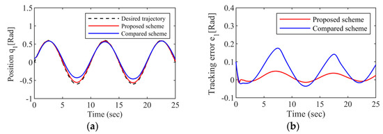
Figure 7.
Tracking performance of joint 1: (a) Tracking trajectory; (b) Tracking error.
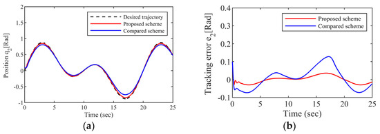
Figure 8.
Tracking performance of joint 2: (a) Tracking trajectory; (b) Tracking error.
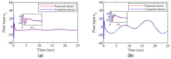
Figure 9.
The actual control input: (a) Joint 1; (b) Joint 2.
Table 4.
Quantity table of tracking error.
Figure 9 shows the actual control input of the system. By the FTOAC, the control input curve is smoother. According to the above analysis, it is clear that the control performance of the FTOAC scheme is much better than the compared scheme.
4.3. The FTOAC under Internal Disturbances from the Drone Platform
In order to verify the FTOAC can tolerate disturbances from the internal force between the arm and the quadrotor, we introduce the following simulation.
Case 1: The system works under the perturbation of internal forces on the robotic arm by the quadrotor UAV, where the disturbances are chosen as
Case 2: The system works under the disturbances and the input saturation .
It can be seen from Figure 10 and Figure 11 that the tracking performance of the system can still be guaranteed by using the FTOAC scheme proposed in this paper in the presence of coupling force interference between the subsystems of the aerial unmanned robotic arm and input saturation. According to Figure 12 and Figure 13, we can see that the unknown disturbances within the system can be approximated by our proposed fixed-time observer within a small time interval.
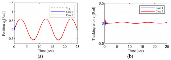
Figure 10.
Tracking performance of joint 1: (a) Tracking trajectory; (b) Tracking error.
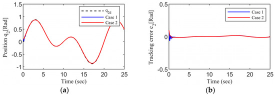
Figure 11.
Tracking performance of joint 2: (a) Tracking trajectory; (b) Tracking error.
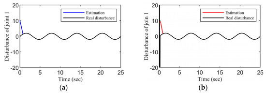
Figure 12.
Disturbance estimation of joint 1 for FTO: (a) Case 1; (b) Case 2.
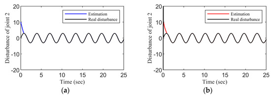
Figure 13.
Disturbance estimation of joint 2 for FTO: (a) Case 1; (b) Case 2.
5. Conclusions
By proposing an FTOAC scheme for the AFJR system, the nonlinear unknown dynamics of the system, the input saturation perturbation problem of the FJR, and the internal disturbances from the UAV are effectively learned and compensated. Then, a tangent-type Lyapunov function is introduced to implement the output constraint, and a fixed-time compensator is designed to eliminate the influences from filtering errors. The stability analysis shows that all the signals of the closed-loop system are bounded, and the system satisfies the condition of fixed-time convergence. The simulation results show that the FTOAC scheme has better control performance than the conventional DSC scheme and can tolerate disturbances from the internal force between the drone and the arm.
Future work will focus on the study of reinforcement learning control problems for AFJR systems and the development of physical platforms.
Author Contributions
Writing—original manuscript preparation, T.L.; Writing—review, editing, and funding acquisition, S.L.; Data curation, H.S.; Writing—review and editing, D.L. All authors have read and agreed to the published version of the manuscript.
Funding
This research was supported in part by the National Key Research and Development Program of China (2018AAA0101800 and 2020YFB1713300), the Guizhou Higher Education Institution Integrated Research Large Platform Project, UAV Test Flight Integrated Research Large Platform ([2020] 005).
Institutional Review Board Statement
Not applicable.
Informed Consent Statement
Not applicable.
Data Availability Statement
The data will be made available upon reasonable request.
Conflicts of Interest
The authors declare no conflict of interest.
Appendix A
Proof of Theorem 1. By taking the derivative of , one can obtain
Letting we have
Taking the derivative of provides
As a result, the error dynamics of the observer for Δ can be represented as
On the basis of the result presented in [50], when the observer gains , , and satisfy the condition (23), and can uniformly converge to the origin within a fixed time as
where . The minimum value of is obtained as long as . Recalling the definition it is proven that can approach within a fixed time.
References
- Ruggiero, F.; Lippiello, V.; Ollero, A. Aerial Manipulation: A Literature Review. IEEE Robot. Autom. Lett. 2018, 3, 1957–1964. [Google Scholar] [CrossRef]
- Xu, M.; Hu, A.; Wang, H. Image-Based Visual Impedance Force Control for Contact Aerial Manipulation. IEEE Trans. Autom. Sci. Eng. 2022, 20, 518–527. [Google Scholar] [CrossRef]
- Kobilarov, M. Nonlinear Trajectory Control of Multi-Body Aerial Manipulators. J. Intell. Robot. Syst. Theory Appl. 2014, 73, 679–692. [Google Scholar] [CrossRef]
- Rsetam, K.; Cao, Z.; Wang, L.; Al-Rawi, M.; Man, Z. Practically Robust Fixed-Time Convergent Sliding Mode Control for Underactuated Aerial Flexible JointRobots Manipulators. Drones 2022, 6, 428. [Google Scholar] [CrossRef]
- Liu, Y.C.; Huang, C.Y. DDPG-Based Adaptive Robust Tracking Control for Aerial Manipulators With Decoupling Approach. IEEE Trans. Cybern. 2022, 52, 8258–8271. [Google Scholar] [CrossRef]
- Montoya-Cháirez, J.; Moreno-Valenzuela, J.; Santibáñez, V.; Carelli, R.; Rossomando, F.G.; Pérez-Alcocer, R. Combined Adaptive Neural Network and Regressor-Based Trajectory Tracking Control of Flexible Joint Robots. IET Control Theory Appl. 2022, 16, 31–50. [Google Scholar] [CrossRef]
- Machado, O.; Rodriguez, F.J.; Bueno, E.J.; Martin, P. A Neural Network-Based Dynamic Cost Function for the Implementation of a Predictive Current Controller. IEEE Trans. Ind. Informatics 2017, 13, 2946–2955. [Google Scholar] [CrossRef]
- Yu, X.; Li, Y.; Zhang, S.; Xue, C.; Wang, Y. Estimation of Human Impedance and Motion Intention for Constrained Human–Robot Interaction. Neurocomputing 2020, 390, 268–279. [Google Scholar] [CrossRef]
- Yang, Y.; Huang, D.; Jin, C.; Liu, X.; Li, Y. Neural Learning Impedance Control of Lower Limb Rehabilitation Exoskeleton with Flexible Joints in the Presence of Input Constraints. Int. J. Robust Nonlinear Control 2022, 33, 4191–4209. [Google Scholar] [CrossRef]
- Wang, H.; Peng, W.; Tan, X.; Sun, J.; Tang, X.; Chen, I.M. Robust Output Feedback Tracking Control for Flexible-Joint Robots Based on CTSMC Technique. IEEE Trans. Circuits Syst. II Express Briefs 2021, 68, 1982–1986. [Google Scholar] [CrossRef]
- Zaare, S.; Reza, M. Continuous Fuzzy Nonsingular Terminal Sliding Mode Control of Flexible Joints Robot Manipulators Based on Nonlinear Finite Time Observer in the Presence of Matched and Mismatched Uncertainties. J. Franklin Inst. 2020, 357, 6539–6570. [Google Scholar] [CrossRef]
- Xie, Y.; Ma, Q.; Gu, J.; Zhou, G. Event-Triggered Fixed-Time Practical Tracking Control for Flexible-Joint Robot. IEEE Trans. Fuzzy Syst. 2022, 31, 67–76. [Google Scholar] [CrossRef]
- Binazadeh, S.; Ghasemi, R. Distributed Fixed Time Super-Twisting Sliding Mode Leader–Follower Tracking Protocol Design for Nonlinear Networked Flexible Joint Robots. Int. J. Dyn. Control 2020, 8, 908–916. [Google Scholar] [CrossRef]
- Ma, H.; Ren, H.; Zhou, Q.; Li, H.; Member, S.; Wang, Z. Observer-Based Neural Control of N -Link Flexible-Joint Robots. IEEE Trans. NEURAL NETWORKS Learn. Syst. 2022, 1–11. [Google Scholar] [CrossRef]
- Liu, Y.; Li, Z.; Su, H.; Su, C.Y. Whole-Body Control of an Autonomous Mobile Manipulator Using Series Elastic Actuators. IEEE/ASME Trans. Mechatronics 2021, 26, 657–667. [Google Scholar] [CrossRef]
- Liu, X.; Zhao, F.; Ge, S.S.; Wu, Y.; Mei, X. End-Effector Force Estimation for Flexible-Joint Robots with Global Friction Approximation Using Neural Networks. IEEE Trans. Ind. Informatics 2019, 15, 1730–1741. [Google Scholar] [CrossRef]
- Liu, X.; Yang, C.; Chen, Z.; Wang, M.; Su, C.Y. Neuro-Adaptive Observer Based Control of Flexible Joint Robot. Neurocomputing 2018, 275, 73–82. [Google Scholar] [CrossRef]
- Wang, H.; Kang, S.; Zhao, X.; Xu, N.; Li, T. Command Filter-Based Adaptive Neural Control Design for Nonstrict-Feedback Nonlinear Systems With Multiple Actuator Constraints. IEEE Trans. Cybern. 2022, 52, 12561–12570. [Google Scholar] [CrossRef]
- Li, Y.X. Finite Time Command Filtered Adaptive Fault Tolerant Control for a Class of Uncertain Nonlinear Systems. Automatica 2019, 106, 117–123. [Google Scholar] [CrossRef]
- Li, K.; Li, Y. Adaptive Neural Network Finite-Time Dynamic Surface Control for Nonlinear Systems. IEEE Trans. Neural Networks Learn. Syst. 2021, 32, 5688–5697. [Google Scholar] [CrossRef]
- Ma, M.; Wang, T.; Guo, R.; Qiu, J. Neural Network-Based Tracking Control of Autonomous Marine Vehicles with Unknown Actuator Dead-Zone. Int. J. Robust Nonlinear Control 2022, 32, 2969–2982. [Google Scholar] [CrossRef]
- Wang, Y.; Xu, N.; Liu, Y.; Zhao, X. Adaptive Fault-Tolerant Control for Switched Nonlinear Systems Based on Command Filter Technique. Appl. Math. Comput. 2021, 392, 125725. [Google Scholar] [CrossRef]
- Wang, L.; Chen, C.L.P.; Li, H. Event-Triggered Adaptive Control of Saturated Nonlinear Systems with Time-Varying Partial State Constraints. IEEE Trans. Cybern. 2020, 50, 1485–1497. [Google Scholar] [CrossRef] [PubMed]
- Ding, S.; Peng, J.Z.; Zhang, H.; Wang, Y.N. Neural Network-Based Adaptive Hybrid Impedance Control for Electrically Driven Flexible-Joint Robotic Manipulators with Input Saturation. Neurocomputing 2021, 458, 99–111. [Google Scholar] [CrossRef]
- Ma, Z.; Huang, P. Adaptive Neural-Network Controller for an Uncertain Rigid Manipulator With Input Saturation and Full-Order State Constraint. IEEE Trans. Cybern. 2022, 52, 2907–2915. [Google Scholar] [CrossRef]
- Cheng, X.; Zhang, Y.; Liu, H.; Wollherr, D.; Buss, M. Adaptive Neural Backstepping Control for Flexible-Joint Robot Manipulator with Bounded Torque Inputs. Neurocomputing 2021, 458, 70–86. [Google Scholar] [CrossRef]
- Yang, Z.; Li, S.; Yu, D.; Chen, C.L.P. BLS-Based Formation Control for Nonlinear Multi-Agent Systems with Actuator Fault and Input Saturation. Nonlinear Dyn. 2022, 109, 2657–2673. [Google Scholar] [CrossRef]
- Zhang, R.; Xu, B.; Shi, P. Finite Time Observer-Based Output Feedback Control of MEMS Gyroscopes with Input Saturation. Int. J. Robust Nonlinear Control 2022, 32, 4300–4317. [Google Scholar] [CrossRef]
- Liu, L.; Hong, M.; Gu, X.; Ding, M.; Guo, Y. Fixed-Time Anti-Saturation Compensators Based Impedance Control with Finite-Time Convergence for a Free-Flying Flexible-Joint Space Robot. Nonlinear Dyn. 2022, 109, 1671–1691. [Google Scholar] [CrossRef]
- Yao, W.; Guo, Y.; Wu, Y.F.; Guo, J. Robust Adaptive Dynamic Surface Control of Multi-Link Flexible Joint Manipulator with Input Saturation. Int. J. Control. Autom. Syst. 2022, 20, 577–588. [Google Scholar] [CrossRef]
- Liu, L.; Yao, W.; Guo, Y. Prescribed Performance Tracking Control of a Free-Flying Flexible-Joint Space Robot with Disturbances under Input Saturation. J. Franklin Inst. 2021, 358, 4571–4601. [Google Scholar] [CrossRef]
- Hu, Y.; Dian, S.Y.; Guo, R.; Li, S.C.; Zhao, T. Observer-Based Dynamic Surface Control for Flexible-Joint Manipulator System with Input Saturation and Unknown Disturbance Using Type-2 Fuzzy Neural Network. Neurocomputing 2021, 436, 162–173. [Google Scholar] [CrossRef]
- Kim, S.; Seo, H.; Kim, H.J. Multirotors With Multi-DOF Robotic Arms. IEEE/ASME Trans. Mechatron. 2018, 23, 702–713. [Google Scholar] [CrossRef]
- Emami, S.A.; Banazadeh, A. Simultaneous Trajectory Tracking and Aerial Manipulation Using a Multi-Stage Model Predictive Control. Aerosp. Sci. Technol. 2021, 112, 106573. [Google Scholar] [CrossRef]
- Yu, X.; He, W.; Li, H.; Sun, J. Adaptive Fuzzy Full-State and Output-Feedback Control for Uncertain Robots with Output Constraint. IEEE Trans. Syst. Man, Cybern. Syst. 2021, 51, 6994–7007. [Google Scholar] [CrossRef]
- Zhang, J.X.; Yang, G.H. Fault-Tolerant Output-Constrained Control of Unknown Euler–Lagrange Systems with Prescribed Tracking Accuracy. Automatica 2020, 111, 108606. [Google Scholar] [CrossRef]
- Wang, A.; Liu, L.; Qiu, J.; Feng, G. Event-Triggered Adaptive Fuzzy Output-Feedback Control for Nonstrict-Feedback Nonlinear Systems With Asymmetric Output Constraint. IEEE Trans. Cybern. 2022, 52, 712–722. [Google Scholar] [CrossRef]
- Sun, W.; Su, S.F.; Xia, J.; Nguyen, V.T. Adaptive Fuzzy Tracking Control of Flexible-Joint Robots with Full-State Constraints. IEEE Trans. Syst. Man, Cybern. Syst. 2019, 49, 2201–2209. [Google Scholar] [CrossRef]
- He, W.; Yan, Z.; Sun, Y.; Ou, Y.; Sun, C. Neural-Learning-Based Control for a Constrained Robotic Manipulator With Flexible Joints. IEEE Trans. Neural Networks Learn. Syst. 2018, 29, 5993–6003. [Google Scholar] [CrossRef]
- Yang, K.; Zhao, L. Command-Filter-Based Backstepping Control for Flexible Joint Manipulator Systems with Full-State Constrains. Int. J. Control. Autom. Syst. 2022, 20, 2231–2238. [Google Scholar] [CrossRef]
- Ouyang, Y.; Dong, L.; Wei, Y.; Sun, C. Neural Network Based Tracking Control for an Elastic Joint Robot with Input Constraint via Actor-Critic Design. Neurocomputing 2020, 409, 286–295. [Google Scholar] [CrossRef]
- Ling, S.; Wang, H.; Liu, P.X. Adaptive Fuzzy Dynamic Surface Control of Flexible-Joint Robot Systems with Input Saturation. IEEE/CAA J. Autom. Sin. 2019, 6, 97–106. [Google Scholar] [CrossRef]
- Samadikhoshkho, Z.; Lipsett, M. Decoupled Control Design of Aerial Manipulation Systems for Vegetation Sampling Application. Drones 2023, 7, 110. [Google Scholar] [CrossRef]
- Izadbakhsh, A. Robust Control Design for Rigid-Link Flexible-Joint Electrically Driven Robot Subjected to Constraint: Theory and Experimental Verification. Nonlinear Dyn. 2016, 85, 751–765. [Google Scholar] [CrossRef]
- Wang, H.; Xu, K.; Qiu, J. Event-Triggered Adaptive Fuzzy Fixed-Time Tracking Control for a Class of Nonstrict-Feedback Nonlinear Systems. IEEE Trans. Circuits Syst. I Regul. Pap. 2021, 68, 3058–3068. [Google Scholar] [CrossRef]
- Yao, Y.; Tan, J.; Wu, J.; Zhang, X. Event-Triggered Fixed-Time Adaptive Fuzzy Control for State-Constrained Stochastic Nonlinear Systems without Feasibility Conditions. Nonlinear Dyn. 2021, 105, 403–416. [Google Scholar] [CrossRef]
- Diao, S.; Sun, W.; Su, S.F.; Xia, J. Adaptive Fuzzy Event-Triggered Control for Single-Link Flexible-Joint Robots With Actuator Failures. IEEE Trans. Cybern. 2021, 52, 7231–7241. [Google Scholar] [CrossRef]
- Sun, Y.; Zhang, L. Fixed-Time Adaptive Fuzzy Control for Uncertain Strict Feedback Switched Systems. Inf. Sci. (Ny). 2021, 546, 742–752. [Google Scholar] [CrossRef]
- Zhang, J.; Niu, B.; Wang, D.; Wang, H.; Zhao, P.; Zong, G. Time-/Event-Triggered Adaptive Neural Asymptotic Tracking Control for Nonlinear Systems with Full-State Constraints and Application to a Single-Link Robot. IEEE Trans. Neural Networks Learn. Syst. 2022, 33, 6690–6700. [Google Scholar] [CrossRef]
- Basin, M.; Panathula, C.B.; Shtessel, Y. Multivariable Continuous Fixed-Time Second-Order Sliding Mode Control: Design and Convergence Time Estimation. IET Control Theory Appl. 2017, 11, 1104–1111. [Google Scholar] [CrossRef]
Disclaimer/Publisher’s Note: The statements, opinions and data contained in all publications are solely those of the individual author(s) and contributor(s) and not of MDPI and/or the editor(s). MDPI and/or the editor(s) disclaim responsibility for any injury to people or property resulting from any ideas, methods, instructions or products referred to in the content. |
© 2023 by the authors. Licensee MDPI, Basel, Switzerland. This article is an open access article distributed under the terms and conditions of the Creative Commons Attribution (CC BY) license (https://creativecommons.org/licenses/by/4.0/).