The Second Derivative of the NDVI Time Series as an Estimator of Fresh Biomass: A Case Study of Eight Forage Associations Monitored via UAS

Abstract

The estimation of crop yield is a compelling and highly relevant task in the scenario of the challenging climate change we are facing. With this aim, a reinterpretation and a simplification of the Food and Agriculture Organization (FAO) fundamentals are presented to calculate the fresh biomass of forage crops. A normalized difference vegetation index (NDVI) series observed from a multispectral camera on board an unmanned aircraft system (UAS) was the basis for the estimation. Eight fields in Spain of different rainfed intercropping forages were flown over simultaneously, with eight field measurements from February to June 2020. The second derivative applied to the NDVI time series determined the key points of the growing cycle, whereas the NDVI values themselves were integrated and multiplied by a standardized value of the normalized water productivity (WP*). The scalability of the method was tested using two scales of the NDVI values: the point scale (at the precise field measurement location) and the plot scale (mean of 400 m²). The resulting fresh biomass and, therefore, the proposal were validated against a dataset of field-observed benchmarks during the field campaign. The agreement between the estimated and the observed fresh biomass afforded a very good prediction in terms of the determination coefficient (R², that ranged from 0.17 to 0.85) and the agreement index (AI, that ranged from 0.55 to 0.90), with acceptable estimation errors between 10 and 30%. The best period to estimate fresh biomass was found to be between the second fortnight of April and the first fortnight of May.

1. Introduction

In the current climate change scenario, the prediction and estimation of crop production in terms of biomass or yield are paramount tasks for the agricultural scientific community; these have become urgent and highly important objectives in the response on the global scale to the food demands of a growing world population [1].

Crops whose productivity depends on the amount of plant biomass usually belong among forage cultivars, which are considered the main feed source for ruminants. These animals are capable of transforming an initially poor-quality foodstuff, generally cereal-based forages with a low protein content, into high-quality products for human consumption, such as milk and meat [2]. Thus, the improvement of forage quality can be translated into the optimization of animal productivity; thereby, more inefficient and unsustainable practices, such as purchasing protein supplements, can be avoided [3]. In this context, intercropping systems, i.e., the simultaneous growth of two or more species [4] in which cereal and legume species are combined, have emerged as a sustainable alternative that may be used to increase the quality and quantity of forages [5]. In contrast to grain crops, these forages are usually harvested with a certain moisture content and have the best nutritional properties; thus, their yields are quantified primarily in terms of fresh plant biomass.

Among the many methods for producing crop statistics described by the Food and Agriculture Organization (FAO) [6], the yield and biomass statistics are usually gathered using crop cuts and/or farmer declarations. During highly expensive surveys, experts may sample subplots within the plot and measure the production by area. This may include visual estimations and the giving of questionnaires to farmers. Alternatively, farmers may be requested to provide a post-harvest estimation of the production in a given area, although visits to parcels and granaries are common. The complexity of estimating biomass over mixed crops is even higher, since intercrops involve two or more crops growing in the same field. In this context, remote sensing and modeling approaches are emerging as alternative procedures to crop production or yield [6].

The FAO has also promoted global initiatives to facilitate the study and applications of the relationship between crop yield and water use by publishing comprehensive guides about the generic topic of “irrigation and drainage”, namely, paper 24: “Crop water requirements” [7], paper 33: “Yield response to water” [8], and paper 66: “Crop yield response to water” [9]. All of these publications attempt to assist farmers and agricultural managers in implementing effective agricultural practices to enhance yield while preserving water consumption. In particular, the FAO paper 66 relies on the AquaCrop model to simulate biomass and yield [10]. AquaCrop belongs to a model group that addresses crop biomass productivity in relation to water availability [11]. Therefore, it is a so-called water-driven model based on the concept of water productivity (WP). The conceptual equation at the core of AquaCrop states that biomass production is proportional to the cumulative amount of water transpired [12]. Since its launch, AquaCrop has been at the core of many studies [13,14,15], including a specific version supported by geographical information systems and remote sensing [16,17]. In fact, the new developments are mainly oriented toward remote sensing data assimilation, which provides the missing spatial information required [18].

However, other larger groups of models exist, either carbon-driven or solar-driven, in which the growth (and, therefore, biomass) estimations are based on carbon or light assimilation, respectively. A ten-year review of AquaCrop [18] performed a thorough and up-to-date revision of different families of models, with many examples. Far from physical modeling, other statistical approaches to predict yield and water production are also nurtured by satellite imagery. Simple or multiple regression models relating remote sensing data features with productivity are still in use [19,20] since they are the simplest and easiest methods to compute, although the results are often inconsistent and not easy to generalize [21]. More sophisticated artificial intelligence techniques from the fields of machine and deep learning, which apply algorithms based on convolutional neural networks, support vector machines, random forest, etc., have been progressively implemented owing to the increasing availability of large and high-quality datasets [21]. The work of van Klompenburg et al. (2020) [22] presents a systematic literature review of these crop yield prediction alternatives.

As ground-based phenological observations are limited, phenology derived from remote sensing can be used as an alternative to parameterize phenological models [23]. Remote sensing data offer many advantages in crop prediction. First and foremost, the images provide a wide spatial range and scalability; they are spatially seamless and may fill in situ data gaps [24]. Second, satellite data can provide a synoptic overview of actual growing conditions and can be used to diagnose discrepancies from normal conditions [25]. Finally, remote data assimilation allows different alternatives: direct substitution of the model parameters, calibration/initialization, or sequential assimilation of algorithms and models [26,27]. In particular, in AquaCrop, the remote sensing inputs are usually assimilated as either indicators or surrogates of the model parameters and include the data (or their derivative products) of remotely sensed temperature, vegetation indices, leaf area indices, soil moisture, the fraction of photosynthetically active radiation, and many others [27,28,29,30,31]. Other examples use satellite data to calibrate AquaCrop inputs [28,32,33], and in other cases, the remotely sensed time series provides the temporal metrics of the growing cycle, such as the start, end, or length of the growing season [16,30].

Among the many remote sensing products, the normalized difference vegetation index (NDVI) [34] seems to be the most popular input in crop production simulation models. The NDVI is simple and easy to interpret and is readily available from most satellite providers [32]. In addition, all multispectral commercial cameras on board unmanned aerial systems (UAS) include red and infrared bands, which are the basis of its calculation [35]. Many examples of yield estimation through UAS observations have also been proposed [35,36,37]. These platforms provide a superhigh spatial resolution but present the disadvantage of their lack of an automatic revisit, as in the case of satellites. Occasionally, this might hamper the monitoring of the complete growing cycle, including the key moments of crop development or senescence.

All applications of the NDVI for yield, biomass, or water productivity are related to the well-known fit between the NDVI time evolution and the growing cycle and phenology of many crops [35,38,39]. Therefore, the NDVI has been used as an effective indicator of crop yield or plant biomass [20,40,41] from different perspectives, such as the direct correlation or the aforementioned assimilation modeling. The shape of the NDVI curve and the particular features of it, such as the integrated, maximum, and moving average or the relative range, have been used as synoptic indicators of biomass or production [19,20]. As another indicator, the second derivative of the NDVI curve has been used for estimating phenological information such as the start of the growing season [42], while its maximum has been related to the beginning of the green-up phase [23,43]. The inflection points resulting from the second derivative of the NDVI curve have inspired our hypothesis on the determination of the period in which the biomass is produced, together with the NDVI value itself.

A novel and simple method was proposed to estimate the fresh biomass of several forage associations based on the joint use of the FAO66 guidelines regarding water productivity together with a temporal series of UAS imagery. The validation of the approach was performed after a field campaign to determine the direct measurements of the biomass that were coincident with those of the flights. The novelty of our proposal lies in (1) the use of the second derivative to determine the period in which the biomass is produced and (2) the replacement of the crop transpiration coefficient with the NDVI summation as a synoptic value of the crop and its status. The calculation is totally independent of any AquaCrop software: only the second derivative and summation of the NDVI series are needed. The detailed scale of the UAS imagery, together with the comprehensive dataset of field measurements, could help to validate the approach in a robust manner. Ultimately, since the majority of the parameterizations used in biomass estimations are only available for single crops, this research enabled the study and comparison of the biomass estimation among eight intercropping forage mixtures, including cereals (rye, triticale, oats, and barley) and legumes (vetch and pea).

2. Materials and Methods

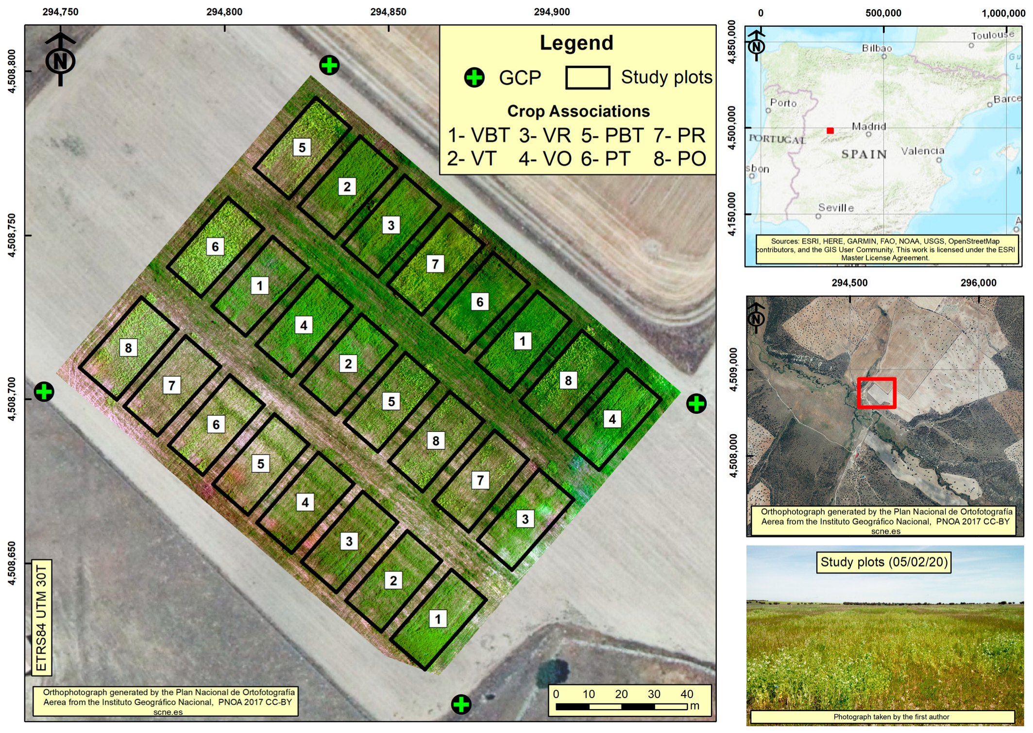
2.1. Study Area

The field experiment was carried out on the organic farm “Gallegos de Crespes” (40°42′13″ N–5°25′43″ W), located in the southwestern part of the province of Salamanca (Castilla y León, Spain) in a typical semiarid rangeland area, commonly known as “dehesa” (Figure 1). The field measurements and flights were conducted during the rainfed growing season of 2019–2020, i.e., from February to June. The geographical area has a continental Mediterranean climate, characterized by a high thermal range between short, hot summers and long, cold winters, very scarce precipitation (350–400 mm/year on average), and a frost period that extends from October to April.

Table 1. Meteorological conditions of the rainfed growing season in the study area.

Parameter	October 2019–June 2020
Mean temperature (°C)	9.5
Total precipitation (mm)	380.2
Spring precipitation (mm)	121.3
Average relative moisture (%)	81.1
Total solar radiation (MJ/m2)	3893.1

Data provided by the Spanish Meteorological Agency (AEMET).

shows the meteorological conditions of the studied period: the values were within the normal ranges for these climatic conditions. Therefore, it could be assumed that the potential yields of the forage associations during the period of study were not affected by weather conditions that differed from those of the expected average. Sandy–clay–loam soils characterize the edaphic conditions, which are developed over arkosic sandstones and are typically of slight acidity (pH 5.5–6.0).

The eight forage associations were constructed from the combination of six forage crops: vetch (Vicia sativa cv. “Rada”); pea (Pisum sativum cv. “Cabestrón”); triticale (Triticum × Secale cv. “Elleac”); six-row barley (Hordeum vulgare ssp. Hexastichum cv. “Yuriko”); rye (Secale cereale cv. “Serafino”); and oat (Avena sativa cv. RGT “Chapela”). Overall, four vetch-based and four pea-based associations, sown at a rate of 140 kg/ha (70% legume–30% cereal) and 130 kg/ha (60% legume–40% cereal), respectively, were proposed: vetch–barley–triticale (VBT); vetch–triticale (VT); vetch–rye (VR); vetch–oats (VO); pea–barley–triticale (PBT); pea–triticale (PT); pea–rye (PR); and pea–oats (PO). Each association was grown in triplicate in a randomized block design of 24 experimental plots of 400 m² each, accounting for a total surface width of one hectare flown over by the drone [44]. However, the field measurements of fresh biomass were only available for the first eight rows of plots, and therefore, a biomass estimation was conducted for these eight fields (Figure 1).

2.2. UAS and Direct Measurements

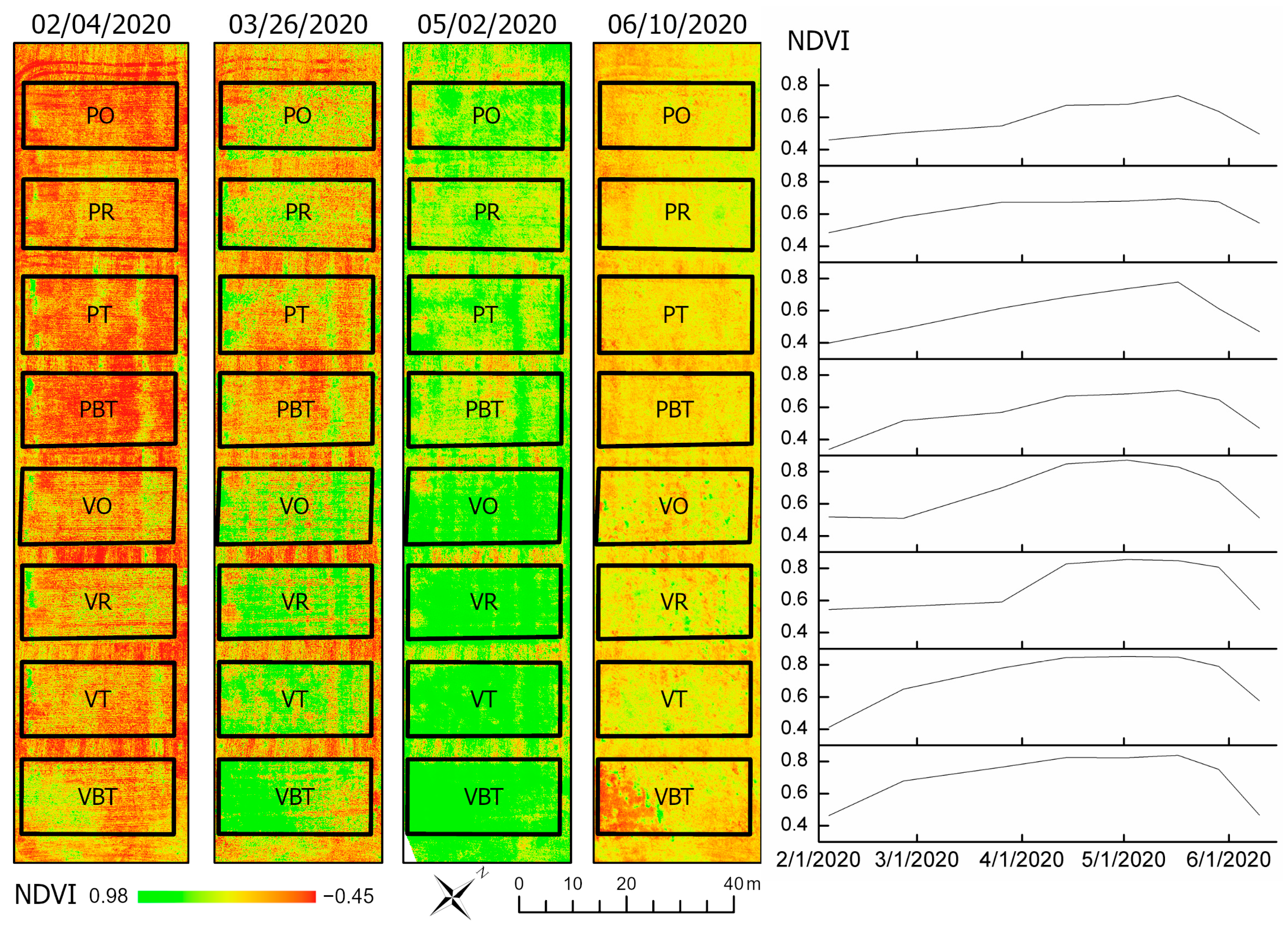
During the growing cycle of the associations, eight UAS flights were conducted on the dates 2/4/2020, 2/26/2020, 3/26/2020, 4/14/2020, 5/2/2020, 5/17/2020, 5/29/2020, and 6/10/2020. The drone mission was the same for each date, and all drones were flown around midday (to avoid shadows) using the flight planning software (DJI GS Pro and Pix4Dcapture). The flight duration was approximately 12 min.

Jointly with the flights, eight field campaigns were deployed in the first eight fields, 1–8 (Figure 1). These dates were selected to depict the key stages of the growing cycle, especially in April and May, when the main phenological changes take place.

2.2.1. UAS Imagery

The drone model was an Inspire1 from the DJI company (SZ DJI Technology Co., Ltd., Shenzhen, China), with a Micasense Red Edge M camera (AgEagle Sensor Systems Inc., d/b/a MicaSense, Wichita, KS, USA) on board [44]. This camera has an image resolution of 1280 × 960 pixels and captures a maximum of one image per second. The image spatial resolution was set to 3 cm, resulting in a flight at a height of 43 m. The camera was mounted in the drone using an in-house-made gimbal and included the GPS receiver and the downwelling light sensor (DLS, MicaSense Inc., Seattle, WA, USA). The DLS faces skyward to embed the solar irradiance data in the multispectral imagery spectrum during the flights [45], allowing the normalization of the varying illumination and thereby automatically adjusting the camera exposure. A calibrated reflectance panel completed the UAS equipment, which ensured a radiometrically corrected reflectance retrieval by taking images of it before and after each flight. The treatment of the images was performed in Pix4D Mapper software (Pix4D P.A., Prilly, Switzerland) using a customized template that included the radiometric calibration and the retrieval of the corrected reflectance maps together with the vegetation indices. In addition to the radiometric correction, geometric correction and ortho-mosaicking were performed by means of four permanent ground control points (GCPs) installed over the flight area (Figure 1, in green). Those points were then geolocated to georeference the images in the Pix4D mapper with centimetric errors. To do so, real-time kinematic (RTK) observations were recorded using a 1200 Leica GPS receiver (Leica Geosystems, Heerbrugg, Switzerland), whereas a local network service provided data from a reference station close to the area. The GPS equipment is described in Plaza et al. (2022) [46].

At each date, the images were registered and input into the Pix4DMapper, which transformed them into five reflectance maps, one per band. The radiometric and geometric corrections ensured a fair comparison of the maps from each date. Previous results obtained with the same dataset in Plaza et al. (2021) [44] suggested that the vegetation index that best followed the growing cycle in terms of biomass was the NDVI. Therefore, eight NDVI maps were composed from February to June (Figure 2) as the cornerstone for the biomass estimation. The NDVI was computed as the difference between the infrared and the red reflectances divided by the sum of both reflectances.

2.2.2. Field: Fresh Biomass in Eight Fields

All the methods performed during the study were conducted in accordance with the relevant guidelines and legislation. This experiment was conducted within the framework of a research project funded by the local government (see acknowledgements). Therefore, prior to the establishment of the experimental design and sample collection, the owners of the “Gallegos de Crespes” organic farm were included as collaborating members of the project; therefore, they gave their explicit permission to collect plants on their land.

Among other parameters, field estimations of fresh biomass were gathered during the eight flights through destructive sampling. Plants within a fenced area of 1/8 m² were cut, immediately fresh-weighed (gr/m²), and subsequently dry-weighed after being dried in an oven at 60 °C for 48 h until they were of a constant weight (dry biomass, gr/m²). The difference between the fresh and the dry biomass, expressed in %, was the percentage of water content, PWC (%). Two measurements were taken at each field and geolocated with the GPS and later averaged for each field and association. The measurements for the date 6/10/2020 were not used in this analysis, since the focus of the research was the fresh biomass, and at that date, the associations were in the senescence phase (the PWC was less than 50% for all the associations).

2.3. The WP* K_c,Tr Approach

The FAO66 methodology [9] estimates the biomass (g/m²) as the product of the normalized water productivity (${WP}^{\mathrm{*}}$, in g/m²) times the summation of the ratio between the crop transpiration ($T_r$, in mm) and the reference evapotranspiration (${ET}_0$, in mm) (Equation (1)). ${WP}^{\mathrm{*}}$ is the biomass water productivity normalized for climate (depending upon the location, season, and CO₂ concentrations). The normalization with respect to the location and season is obtained by dividing the daily amount of water transpired ($T_r$) by the reference evapotranspiration (${ET}_0$) for that day [12]. The normalization for CO₂ consists of considering the water productivity for a reference atmospheric CO₂ concentration of 369.41 ppm [12]. ${WP}^{\mathrm{*}}$ remains virtually constant over a range of environments and crops and is 18 g/m² for many crops [9,30]. The temporal limits $t_0$ and $t$ of the summation (with daily intervals) must be known.

$$B={WP}^{\mathrm{*}}\sum _{t_0}^t\frac{T_r}{{ET}_0}$$

(1)

$$B={WP}^{\mathrm{*}}\sum _{t_0}^t{K}_{c,Tr}$$

(2)

The ratio of $T_r$ to ${ET}_0$ is equivalent to the crop transpiration coefficient, denoted by $K_{c,Tr}$ and defined as the crop coefficient for transpiration “when the canopy fully covers the ground and stresses are absent” [9] (Equation (2)). In AquaCrop, this equation is inserted into a complete set of additional model components, including the characteristics and calculations pertaining to soil, crop, climate, and management [10]. In addition, stress conditions (water supply, temperature, soil fertility, and salinity, among others) modulate the core equation of AquaCrop by means of a variety of stress coefficients.

A time series of UAS imagery offers an alternative way to monitor $K_{c,Tr}$ during the entire growing season. Whereas $K_{c,Tr}$ has been related to the vegetation indices through a linear equation [30], our approach directly replaces $K_{c,Tr}$ with the NDVI. This solution is based on several analogies between $K_{c,Tr}$ and the NDVI. First, $K_{c,Tr}$ is proportional to the fraction of green canopy cover (CC in AquaCrop) and is thus continuously adjusted. Likewise, the linear relationship between CC and NDVI is well known [47,48,49], and their temporal dynamics are quite similar. Therefore, the NDVI time series seems to be able to threshold the temporal limits of the maximum CC. Second, the numeric limits of $K_{c,Tr}$ and the NDVI are within the same maximum range. Third, as stated before, the biomass calculation should be later refined in AquaCrop, taking into account stress conditions, crop physiology, and management through other coefficients. The NDVI precisely depicts the real state of the crop because it represents the actual response of the plant to the edaphoclimatic conditions, including any kind of stress. The NDVI may be considered a synoptic output of the vegetation activity. Therefore, the direct use of the NDVI might avoid the application of other coefficients.

The core of the proposed biomass calculation is therefore based on the use of the NDVI instead of $K_{c,Tr}$ in Equation (2) and on the estimation of the $t_0$ and $t$ limits of the summation based on the NDVI curve, as explained in the following section.

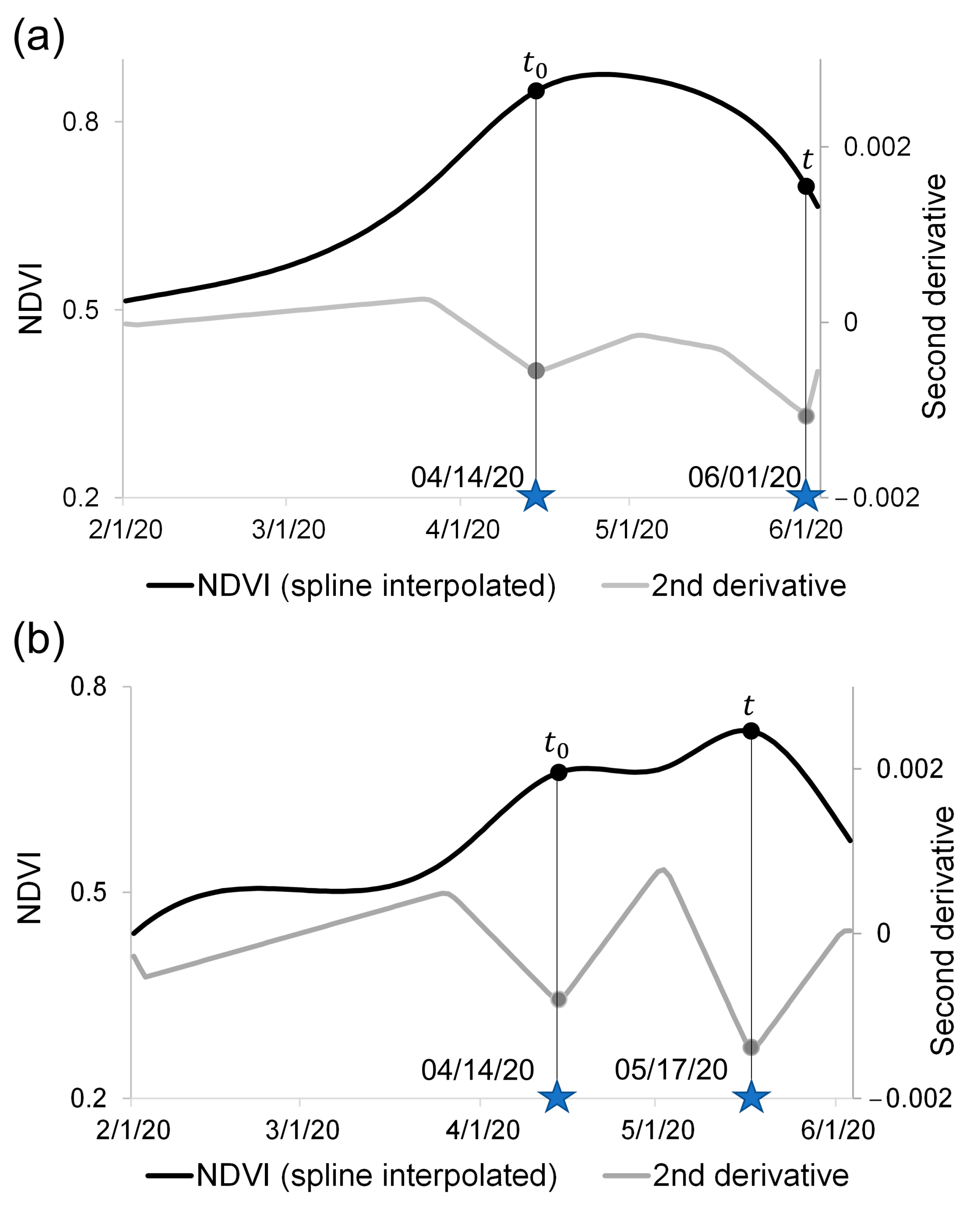
2.4. Use of the NDVI Second Derivative to Retrieve the Temporal Thresholds

The second derivative of a function indicates its curvature or its concavity/convexity. Our hypothesis was that the local minima second derivative may indicate the temporal onset (the day when the maximal convexity in the NDVI is reached and the slope is positive) and offset (the day when the maximal convexity in the NDVI is reached and the slope is negative) of the biomass production (Figure 3). During this period, the green canopy reaches its full development and fully covers the ground to its maturity (as required in the WP* K_c,Tr approach); thus, the NDVI at this stage may represent an estimator of the rate of fresh matter accumulation. After this, the declining phase due to leaf senescence begins.

The eight-point NDVI curve resulting from the flights (Figure 2) was fitted to a spline function prior to computing the second derivative. Then, by scanning the second derivative from the initial growing stages to the end of the cycle, two points of local minimum values of the second derivative were detected. These points correspond to the local maximal downward concavity of the derivative (Figure 3) and, consequently, the maximal convexity of the NDVI curve and were assumed to be the temporal limits of the fresh biomass production period, i.e., $t_0$ and $t$ in Equation (2).

2.5. Scalability

Two spatial resolutions for the NDVI were tested to study the scalability of the proposal:

(a)

At the point scale, the precise location of the ground measurements was used. The NDVI of each date was extracted at each location (two replicates per field) by applying a buffer of the same size as the fenced area used in the field sampling. For each association, the two NDVI values were averaged.

(b)

At the field scale, the NDVI was averaged for each whole experimental plot. The aim of the idea to use an averaged value for an area of 400 m² was to assess the robustness of the approach when using satellite scales, i.e., to estimate biomass production at the regional scale.

2.6. Validation of the Approach

To assess the feasibility of the proposed method, several comparisons between the estimated and the observed fresh biomass were performed. First, an exploratory analysis between the NDVI observations and the biomass measured at each date was conducted using the linear Pearson correlation coefficient, R. The NDVIs of the eight associations were compared to the fresh biomass measured for each plot over time (temporal evolution of NDVI vs. biomass) and at each date (NDVI vs. biomass for the eight associations combined at each date). These correlations aimed to preliminarily analyze which period (if any) of the NDVI series was better suited to retrieving fresh biomass.

The validation was then accomplished by the statistical comparison between the biomass estimations after the WP*NDVI method and the field observations using the following statistics: the mean absolute bias (MAB) (Equation (3)) to measure the difference between the observed and the estimated values; the coefficient of determination R² to measure how well the estimation predicted the fresh biomass; the root-mean-square difference (RMSD) (Equation (4)) to measure the differences between both datasets); and the agreement index (AI) (Equation (5)), which is typically used in hydrological modeling [50] to assess a model predictions. Specifically, the AI varies between 0 (total disagreement between predicted and observed values) and 1 (perfect agreement).

$$\mathrm{M}\mathrm{A}\mathrm{B}=\frac{\sum _{i=1}^n\left|x_i-y_i\right|}{n}$$

(3)

$$\mathrm{R}\mathrm{M}\mathrm{S}\mathrm{D}=\sqrt{\sum _{i=1}^n\frac{{(x_i-y_i)}^2}{n}}$$

(4)

$$\mathrm{A}\mathrm{I}=1-\frac{\sum _{i=1}^n{(x_i-y_i)}^2}{\sum _{i=1}^n{(|x_i-\stackrel{-}{x}|+|y_i-\stackrel{-}{x}|)}^2}$$

(5)

In the above equations, $x_i$ is the observed biomass for a given date for the eight associations, and $y_i$ is their fresh biomass estimated through the WP*NDVI approach. The average for those datasets is indicated by a bar. These statistics were obtained for the two scales of the analysis.

3. Results

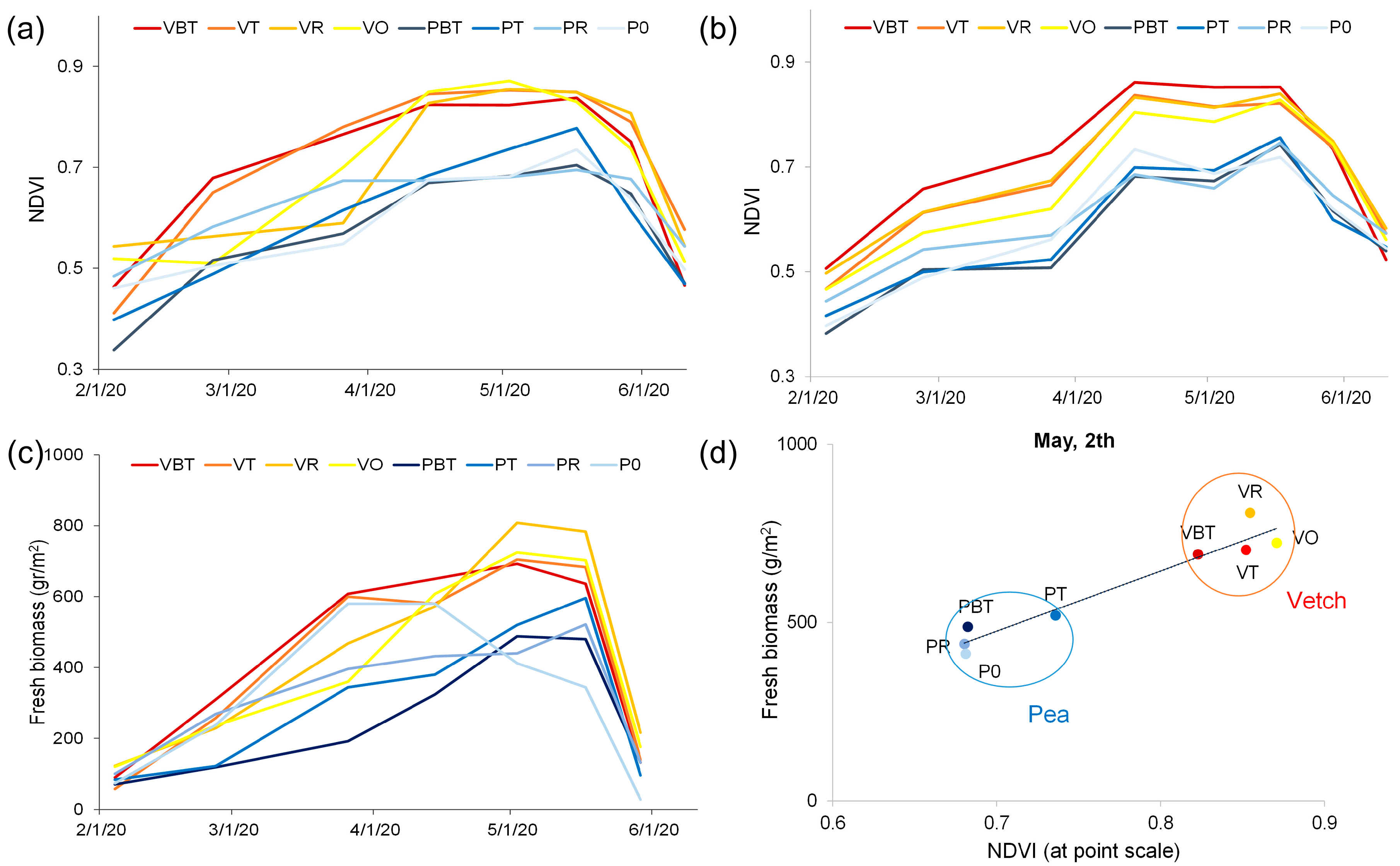
3.1. Exploratory Analysis of the Fresh Biomass–NDVI Relationships

The fresh biomass measurements for each association over time (

Table 2. Fresh biomass (gr/m²) for each association (field measurements).

Fresh Biomass (gr/m2)	VBT	VT	VR	VO	PBT	PT	PR	PO
2/4/2020	90.0	58.0	122.9	120.2	70.9	84.1	100.2	73.8
2/26/2020	309.6	257.3	228.6	236.1	118.9	121.8	268.9	237.6
3/26/2020	608.0	600.0	468.0	360.0	192.0	344.0	396.0	580.0
4/14/2020	650.0	580.0	572.0	608.0	324.0	380.0	232.0	580.0
5/2/2020	692.0	704.0	808.0	724.0	488.0	520.0	440.0	412.0
5/17/2020	636.0	883.0	783.5	772.0	480.0	596.0	621.5	344.0
5/29/2020	132.0	140.0	216.0	176.0	132.0	96.0	132.0	28.0

VBT: vetch–barley–triticale; VT: vetch–triticale; VR: vetch–rye; VO: vetch–oats; PBT: pea–barley–triticale; PT: pea–triticale; PR: pea–rye; and PO: pea–oats.

) showed two main characteristics: (1) a higher biomass for the vetch-based associations and (2) higher values between the second half of April and the first half of May.

The temporal evolution of both the NDVI and the fresh biomass for the eight associations (Figure 4) followed a similar pattern, which was typically shaped as a “plateau” [51,52]. However, a time lag was recognizable between them (except for the PO and VBT curves), which suggests that the time integration of the NDVI values would be a better option to calculate biomass than a direct estimation through the NDVI [53,54]. This temporal shape was also clear for the NDVI calculated at the field scale (Figure 4b), although in this case it was noticeable that the field average smoothed the NDVI, displaying smaller differences between the associations. Nonetheless, in both cases, the vetch-based associations exhibited a higher NDVI and biomass production (Figure 4). In fact, the behaviors of both associations in terms of NDVI and biomass were clearly distinguishable (Figure 4d). For the given example of 2 May in Figure 4d, less biomass, approximately 500 g/m² (5000 kg/ha), was related to a lower NDVI, approximately 0.7 for the associations containing pea, whereas a higher biomass, approximately 700 g/m² (7000 kg/ha), was related to a higher NDVI, approximately 0.85 for the vetch-based associations. These preliminary results suggested that the NDVI was a reasonable indicator of fresh biomass, as hypothesized in the methodology section.

The exploratory correlations between the temporal evolution of fresh biomass and the NDVI (

Table 3. Correlations (R of Pearson) between the temporal evolution of the NDVI and the fresh biomass for the eight associations.

Fresh Biomass vs. NDVI (R)	VBT	VT	VR	VO	PBT	PT	PR	PO
At point scale	0.79 *	0.78 *	0.72	0.85 *	0.77 *	0.88 **	0.70	0.35
At field scale	0.82 *	0.76 *	0.82 *	0.80 *	0.85 *	0.83 *	0.72	0.53

* Significant correlation at the 0.05 level (2-tailed). ** Significant correlation at the 0.01 level (2-tailed). NDVI: normalized difference vegetation index; VBT: vetch–barley–triticale; VT: vetch–triticale; VR: vetch–rye; VO: vetch–oats; PBT: pea–barley–triticale; PT: pea–triticale; PR: pea–rye; and PO: pea–oats.

) showed a good fit, with no remarkable differences between the scales and the associations. The correlation was significant (or very close to significant) for all the associations except for the PO association. This good fit between the temporal curve of the NDVI and that of the fresh biomass triggered the hypothesis of the research, while the aforementioned lag between them suggested the integration of the NDVI values.

The correlations between the NDVI and thefresh biomass calculated separately at each date for the eight associations (

Table 4. Correlations (R of Pearson) between the NDVI and the total fresh biomass of the eight associations on the seven measurement dates.

Fresh Biomass vs. NDVI (R)	2/4/20	2/26/20	3/26/20	4/14/20	5/2/20	5/17/20	5/29/20
At point scale	0.82 *	0.73 *	0.46	0.77 *	0.97 **	0.82 *	0.74 *
At field scale	0.51	0.70	0.72 *	0.87 **	0.91 **	0.88 **	0.72 *

* Significant correlation at the 0.05 level (2-tailed). ** Significant correlation at the 0.01 level (2-tailed). NDVI: normalized difference vegetation index.

) indicated that the highest correlations occurred in April and May and, more specifically, at the beginning of May. These results suggest that the period between April and May might be the best period to calculate the fresh biomass through the NDVI. Again, there were no remarkable differences when changing the NDVI scale of observation.

3.2. Results of $t_0$ and $t$

The second derivative of the NDVI curve afforded the limits $t_0$ and $t$ needed for the integration of the NDVI values. At the point scale, the results for $t_0$ were 14 April for all the associations except for PT. For $t$, it was 1 June for all of them except for PT and PO, for which $t$ was 17 May. Figure 3b and Figure 4a may explain this delay of $t$ for these pea-based associations due to the existence of a second peak in their NDVI curves.

At the field scale, the results for $t_0$ were similar to those at the point scale (14 April) for all the associations. However, $t$ resulted earlier for all of them (18 May for the vetch-based associations and 17 May for the pea-based ones). This difference with respect to the point scale results may be explained once again by the peak of the NDVI curve around these dates (Figure 4b). The similarity of the dates for all the associations could be explained by their similar NDVI curves (Figure 4b), owing to the averaging of the whole field.

3.3. Fresh Biomass Estimation: Regression and Errors

The results of the fresh biomass (kg/ha) estimated through the WP*NDVI method (

Table 5. Fresh biomass estimation through the WP*NDVI method for each association.

Fresh Biomass (kg/ha)	VBT	VT	VR	VO	PBT	PT	PR	PO
At point scale	7144.4	7369.7	7369.5	7294.3	5974.1	4596.5	6005.4	4235.9
At field scale	5381.6	5179.2	5196.9	5048.9	4234.1	4342.2	4204.4	4329.7

VBT: vetch–barley–triticale; VT: vetch–triticale; VR: vetch–rye; VO: vetch–oats; PBT: pea–barley–triticale; PT: pea–triticale; PR: pea–rye; and PO: pea–oats.

) showed differences between the two scales. The field scale afforded a reduced biomass production, which can be explained by the shorter period between $t_0$ and $t$ (from April to May) and the corresponding smaller number of NDVI values integrated in the summation. Moreover, although the difference between the vetch-based and the pea-based production was notable, these differences were more remarkable at the point scale. This result was not surprising, since the NDVIs of the associations were more variable, and consequently, so were the limits of $t_0$ and $t$. Overall, the deviations in the biomass obtained with both scales fit the differences that were also observed in the field measurements (Table 2).

Note that the smaller values of the resulting biomass for PO agreed well with the smaller fresh biomass field observed for the dates of late April and May (Figure 4c, pale blue line, and Table 2) owing to its earlier production compared with the other associations.

The statistical assessment (

Table 6. Statistical comparison between estimated and observed fresh biomass on the dates of April and May (point scale).

Fresh Biomass at Point Scale (kg/ha)	R2	MAB (kg/ha)	MAB (%)	RMSD (kg/ha)	AI
4/14/2020	0.17	1732.3	35.3	1975.2	0.58
5/2/2020	0.73	592.2	9.9	776.1	0.90
5/17/2020	0.69	834.9	13.1	939.5	0.88
5/29/2020	0.73	4933.7	375.2	4997.7	0.14

R², determination coefficient; MAB: mean absolute bias; RMSD: root-mean-square difference; and AI: agreement index.

and

Table 7. Statistical comparison between estimated and observed fresh biomass on the dates of April and May (field scale).

Fresh Biomass at Field Scale (kg/ha)	R2	MAB (kga/ha)	MAB (%)	RMSD (kg/ha)	AI
4/14/2020	0.66	1023.1	20.8	1116.2	0.67
5/2/2020	0.85	1297.8	21.7	1588.1	0.64
5/17/2020	0.51	1877.8	29.4	2125.8	0.55
5/29/2020	0.34	3424.6	260.4	3454.5	0.18

R², determination coefficient; MAB: mean absolute bias; RMSD: root-mean-square difference; and AI: agreement index.

) was conducted on the dates suggested by the previous exploratory analysis, i.e., those of April and May. Whereas the predictions were successful at both scales for the dates 5/2/20 and 5/17/20, the estimation failed for the date 5/29/20, probably because the moisture content and, therefore, the weight of the fresh biomass were notably smaller (Table 2) on this date, which coincided with the beginning of senescence and the NDVI decay. The estimation on 4/14/20, although satisfactory, afforded poorer statistics at the point scale, probably for the same reason, but in the opposite sense: the first half of April appeared as a relatively early period to estimate a final biomass. The dates that exhibited more accurate estimations were 5/2/20 and 5/17/20.

The statistical assessment of the biomass estimation revealed a very good fit in terms of R² and AI for both scales; the fit was slightly better at the point scale, and a very high AI was shown for the first half of May. At the plot scale, the best estimation took place for 5/2/22, and R² and AI were lower for the second half of May, whereas the MAB and RMSD were slightly worse. The MAB ranged from 10 to 30% (except for the end of May) and was remarkably better for the point scale retrieval (10 and 13% of MAB for the dates 5/2/20 and 5/17/20, respectively). In terms of absolute values, the MAB ranged from 592.2 to 1877.8 kg/ha, with all values being positive, i.e., the calculation underestimated the observed values.

4. Discussion

The integration of NDVI values to estimate plant biomass, net primary production, or grain yield is one of the most popular approaches for the remote sensing community [54,55]. The main difficulty of the retrieval based on the NDVI integration lies in (1) choosing the precise time-critical crop growth stages that lead to the final biomass accumulation and (2) searching for these key phenological stages and identifying them over the NDVI time series within which the integration is to be performed. Regarding the first issue, the proposal was made to begin biomass accumulation during the late flowering and maturity stages, as was also suggested by Hassan et al. (2019) [35], rather than at the green-up of the initial development phases, as proposed by many other authors [30,40,54] who sought a sudden increase that might signal the onset of significant photosynthetic activity [55]. This selection is in line with Calera et al. (2004) [51], who selected the NDVI plateau stage coinciding with the linear growth phase as an estimator of the potential rate of matter accumulation. In addition, this choice fits the FAO66 condition of using Kc,Tr when the canopy cover is full, since the NDVI second derivative limits ensure a CC close to 100%.

Regarding the second question, i.e., how to identify the NDVI critical growth stages, thresholds based on the NDVI maxima, averages, or moving averages have frequently been proposed [56,57]. Although these thresholds possess the advantage of being easy to recognize, they are not systematic and can be affected by local conditions, such as vegetation, soil, and illumination [55], as well as by sensor biases. The use of NDVI derivatives, although less frequent in the literature, may overcome these problems. The first, second, and third derivatives were applied to determine the start of the season as the date of the maximum increase in the respective NDVI derivative curve [23,42]. In particular, the maximum of the second derivative has been related to the beginning of the green-up phase [43] or to the time when the majority of pixels are turning green [42]. Our data confirmed that the maximum of the second derivative indicates the downward concavity of the NDVI curve (end of March in Figure 3a,b) and thus also the onset of the green-up. However, our perspective is rather different. The biomass accumulation was produced during a later stage, coinciding with the local minimum of the second derivative and the maximum convexity of the NDVI curve (Figure 3). In particular, in our study, this point corresponded to 14 April. Our proposal agrees with Labus et al. (2002) [58] and Doraiswamy and Cook (1995) [59] in that the early-season NDVI parameters were not consistent indicators of the wheat yields, and the NDVI growth profiles showed a stronger relationship with the yield later in the season during the grain-filling stage. Conversely, at the end of the curve, the green biomass production decayed before the offset of the cycle, in the middle of May, coinciding with the latter minimum of the second derivative. This point would be readily identifiable at the end of the cycle and would allow farmers to harvest during an optimal time of production and forage conditions. The method may also provide an early warning about a potential harvest decline due to adverse weather or crop conditions. In addition, this early-season estimation could not only reduce resource input and environmental pollution, but also increase crop yield and the subsequent profits [60,61], as well as determine inputs such as nutrients, pesticides, and water in order to optimize the yield potential.

While the NDVI has repeatedly been used in AquaCrop as a surrogate of some parameters, including CC or crop coefficients [16,30,31,32], our approach considered the NDVI as a single synoptic indicator of crop vigor, biomass production, and plant status. Supporting this idea, it was shown that the NDVI may include different stresses, such as the impacts of fire, frost, or drought, during sensitive crop stages [25]. Therefore, following the water productivity fundamentals, the integrated NDVI was multiplied by WP* as a constant. In this first attempt, a value of $W{P}^{*}=18 \mathrm{g}\mathrm{r}/{\mathrm{m}}^2$ (180 kg/ha) was chosen based on the literature. However, this value could be adapted to the specific characteristics of the forage associations. As a given example, taking into account that the NDVI maximum is 1, the expected maximum daily productivity would be 180 kg/ha. Furthermore, considering that the number of days ranged between 34 and 50 (depending on the association and the scale), the possible maximum fresh biomass production ranged from 6300 to 9000 kg/ha, which are considered feasible values of forage yield in a semiarid rangeland ecosystem such as the dehesa [62,63]. The actual results for the forage associations ranged from 4200 to 7400 kg/ha (Table 5) and were in line with the observed values and the different behavior observed with respect to the vetch-based and pea-based associations. The accuracy of these estimations in terms of the RMSD (excluding the failed date at the end of May) ranged from 700 to 2000 kg/ha, and the MAB ranged from 600 to 1900 kg/ha (all the values were positive), which represented error percentages ranging from 10 to 30% (Table 6 and Table 7). Although rather high, these numbers are in accordance with other crop biomass/yield estimations that used remote sensing and more complex approaches or models. Ajith et al. (2017) [64] used an integrated NDVI for rice and found error percentages ranging from 11 to 21%. Benedetti and Rossini (1993) [65] found an error from 10 to 19% using cumulative NDVI profiles in a regression model for wheat, and in a similar approach, Doraiswamy and Cook (1995) [59] found much higher and variable errors at the county/regional levels in two regions of the USA. Using the simple algorithm for the yield estimates (SAFY) model for maize with high spatial and temporal resolution remote sensing data, Battude et al. (2016) [66] found a relative error for dry biomass of 14%. Using the same model, Claverie et al. (2012) [67] found a relative error of 25% for maize and of 39% for sunflower. Ji et al. (2022) [68] used three machine learning algorithms for faba beans, obtaining yield estimation errors from 18 to 31%. Many other examples may be cited [69], although most of them present the error in terms of absolute errors of biomass (kg or tons per ha) for a given crop; so, they are hardly comparable to the forage associations studied here, which, in addition, are not frequently studied in the literature. In any case, the estimation may supply a rough estimate of forage biomass for livestock feeding that could otherwise have been difficult to draw from traditional surveys, as also stated by Benedetti and Rossini (1993) [65].

In addition to its simplicity, another relevant advantage that should be emphasized with regard to this approach is its objectivity. Occasionally, the parameterization of a model is applied in a relative manner, through comparison with other users or the same user over time, rather than applied as an absolute value [69]. This objectivity is sustained by the NDVI’s capacity to determine the status and vigor of the plant, which ultimately implies its biomass production capacity. While a higher NDVI value is associated with a faster growth rate and higher biomass accumulation during the vegetative stage [35], this higher NDVI is not always related to a higher grain yield. Nevertheless, there is a deep discussion in the scientific literature about the predictive capacity of the NDVI for biomass or grain yield depending on the developmental stage [40,65,70]. The approach performed reasonably well for fresh or green biomass, but this was not the case for the final biomass estimated at the end of May, when senescence had already initiated. The relationship between the biomass measured on 29 May and the NDVI on the same date for the eight associations showed good agreement in terms of R (Table 4), but substantial differences between the observed and the estimated weights were found on this date (Table 2 and Table 5, respectively). Hence, the MAB and RMSD were unacceptable. It should be highlighted that the focus of the work was the estimation of green forage for livestock feeding at the time of the highest nutritional quality of the forage crops. Hence, the last date was beyond the focus of the research.

In addition, the objectivity of the approach was built upon a new, systematic way to determine the key stages through the second derivative, although much more research should be conducted with other crops, different edaphoclimatic conditions, and remote sensors to validate the hypothesis. As the calculation directly depends on the NDVI values, one essential requirement is a previous, rigorous calibration and correction of the sensor reflectance to ensure a fair integration between the NDVIs from different dates. In this case, the radiometric calibration, together with the correction of the light conditions, guaranteed the stability of the images regardless of the illumination conditions and the sensor characteristics. Another remark that could be made is on the use of the red-edge band of the Micasense camera, profiting from its spectral capacity. However, this band was previously tested in comparison with crop parameters with the same dataset [44], and it was found that the indices based in the red-edge band did not correlate well with structural parameters such as LAI and biomass; however, it seemed better suited to the depiction of chemical parameters, as was also found in another similar research study [71].

The scale of observation is also a key factor to be accounted for. In this work, two scales of NDVI observations were used: point scale (approximately 1/8 m²) and plot scale (approximately 400 m²), both of which were enabled by the superhigh spatial resolution of the images. Other studies have compared regional vs. local results, profiting from the scalability of remote sensing images [58,65,66]. Predictions based on satellite platforms appear to improve with the increased radiometric purity of the pixels [59,65]. In this vein, UAS would seem a perfect alternative because the derived image resolution is much higher than that from satellite systems and because it excludes land cover mixed pixels and atmospheric effects. Our estimations using the UAS resolution were superior in terms of biomass and errors at the point scale, probably because the NDVI values that were strictly bound by the sampling area better fit the field estimations. In fact, when the NDVI was averaged onto a plot scale, the biomass variability between plots was slightly lost, particularly for the pea-based associations (Table 5). However, other authors [53] found that an integrated average NDVI determined using a window size larger than a 1 × 1 pixel improved the results. Considering that regional yield or biomass statistics usually provide an averaged value over large areas, it seems reasonable that the averaged values of the image may better fit those broad statistics. Further applications must then be applied at regional scales to appraise the method’s performance, particularly when using remote sensing sensors such as the Landsat series or Sentinel-2 or recent high-resolution systems such as Geosat-2. These optical sensors may allow long temporal NDVI series to be readily available, affording repeatability and continuous observations instead of labored drone campaigns.

5. Conclusions

There are well-recognized methods for the estimation of crop yield or biomass. Agronomic, physical, or statistical modeling assisted by remote sensing databases aims to estimate the agricultural production. One of the most popular approaches is the growth model developed by the Food and Agricultural Organization, AquaCrop; this model is particularly suited to the simulation of yield based on the response of herbaceous crops to water under limiting conditions. Our proposal implemented the idea of “water productivity” (WP*) from AquaCrop to develop a simple calculation of fresh biomass using an NDVI time series as the main input together with a conventional and accepted value of WP*. The main objective was then to evaluate the feasibility of the methodology when applied at superhigh spatial resolution over rainfed forage associations. The major novelty is the use of the second derivative to define the time limits of biomass production, which in turn demarcated the integration of the NDVI values. The second derivative of the NDVI time series resulted in being a strong indicator of the crop status, determining the key temporal points of the onset and offset of the forage yield and therefore creating an unexplored way to estimate the forage yield. The estimation was successful, with acceptable errors and good predictions. The best period to estimate fresh biomass occurred between the second half of April and the first half of May. During this period, a farmer may decide that the expected forage production is good enough to make the harvesting and haying process economically profitable or, on the contrary, that it would be better for the animals to consume the forage directly from the field, thus avoiding the costs of harvesting in situations with low expected forage yields. It should be highlighted that the method can be useful in estimating fresh biomass even one month before harvesting. Although the approach appeared to be scalable, the biomass estimation with the NDVI series should be supported by other large-scale remote sensors, as well as other single crops under different climatic and agricultural regimes.

References

1. Shem, G.; Kelonye, F. Prediction of Crop Yields under a Changing Climate. In Agrometeorology; Swaroop, R., Ed.; IntechOpen: London, UK, 2021; ISBN 978-1-83881-175-4. [Google Scholar]
2. Ghanbari-Bonjar, A.; Lee, H.C. Intercropped Wheat (Triticum aestivum L.) and Bean (Vicia faba L.) as a Whole-Crop Forage: Effect of Harvest Time on Forage Yield and Quality. Grass Forage Sci. 2003, 58, 28–36. [Google Scholar] [CrossRef]
3. Eskandari, H.; Ghanbari, A.; Javanmard, A. Intercropping of Cereals and Legumes for Forage Production. Not. Sci. Biol. 2009, 1, 7–13. [Google Scholar] [CrossRef]
4. Willey, R.W. Intercropping: Its Importance and Research Needs. Part 1, Competition and Yield Advantages; Field Crop Abstract: Washinton, DC, USA, 1979; Volume 32. [Google Scholar]
5. Belel, M.D.; Halim, R.A.; Rafii, M.Y.; Saud, H.M. Intercropping of Corn with Some Selected Legumes for Improved Forage Production: A Review. J. Agric. Sci. 2014, 6, p48. [Google Scholar] [CrossRef]
6. FAO Handbook on Crop Statistics: Improving Methods for Measuring Crop Area, Production and Yield; Pasetto, L. (Ed.) FAO Statistics Division (ESS): Rome, Italy, 2018. [Google Scholar]
7. Doorenbos, J.; Pruitt, W.O. Crop Water Requirements; Agriculture Organization of the UNited Nations: Rome, Italy, 1977; ISBN 92-5-100279-7. [Google Scholar]
8. Doorenbos, J.; Kassam, A.H. Yield Response to Water; Land and Water Development Division, Food and Agriculture Organization of the UNited Nations: Rome, Italy, 1979; ISBN 92-5-100744-6. [Google Scholar]
9. Steduto, P.; Hsiao, T.C.; Fereres, E.; Raes, D. Crop Yield Response to Water; Food and Agriculture Organization of the United Nations (FAO), Ed.; Food and Agriculture Organization of the United Nations (FAO): Rome, Italy, 2012; ISBN 978-92-5-107274-5. [Google Scholar]
10. Raes, D.; Steduto, P.; Hsiao, T.C.; Fereres, E. AquaCrop—The FAO Crop Model to Simulate Yield Response to Water: II. Main Algorithms and Software Description. Agron. J. 2009, 101, 438–447. [Google Scholar] [CrossRef]
11. Weiss, M.; Jacob, F.; Duveiller, G. Remote Sensing for Agricultural Applications: A Meta-Review. Remote Sens. Environ. 2020, 236, 111402. [Google Scholar] [CrossRef]
12. FAO. Book I: Understanding AquaCrop; Raes, D., Ed.; Food and Agriculture Organization of the United Nations (FAO): Rome, Italy, 2017; ISBN 9789251093900. [Google Scholar]
13. Biazin, B.; Wondatir, S.; Tilahun, G.; Asaro, N.; Amede, T. Using AquaCrop as a Decision-Support Tool for Small-Scale Irrigation Systems Was Dictated by the Institutional and Market Incentives in Ethiopia. Front. Water 2021, 3, 96. [Google Scholar] [CrossRef]
14. Greaves, G.E.; Wang, Y.-M.; Hess, T.; Knox, J. Assessment of FAO AquaCrop Model for Simulating Maize Growth and Productivity under Deficit Irrigation in a Tropical Environment. Water 2016, 8, 557. [Google Scholar] [CrossRef]
15. Heng, L.K.; Hsiao, T.; Evett, S.; Howell, T.; Steduto, P. Validating the FAO AquaCrop Model for Irrigated and Water Deficient Field Maize. Agron. J. 2009, 101, 488–498. [Google Scholar] [CrossRef]
16. Han, C.; Zhang, B.; Chen, H.; Wei, Z.; Liu, Y. Spatially Distributed Crop Model Based on Remote Sensing. Agric. Water Manag. 2019, 218, 165–173. [Google Scholar] [CrossRef]
17. Lorite, I.J.; García-Vila, M.; Santos, C.; Ruiz-Ramos, M.; Fereres, E. AquaData and AquaGIS: Two Computer Utilities for Temporal and Spatial Simulations of Water-Limited Yield with AquaCrop. Comput. Electron. Agric. 2013, 96, 227–237. [Google Scholar] [CrossRef]
18. Salman, M.; García-Vila, M.; Fereres, E.; Raes, D.; Steduto, P. The AquaCrop Model: Enhancing Crop Water Productivity. Ten Years of Development, Dissemination and Implementation 2009–2019; Food and Agriculture Organization of the United Nations (FAO), Ed.; Food and Agriculture Organization of the United Nations (FAO): Rome, Italy, 2021; ISBN 9789251352229. [Google Scholar]
19. Johnson, D.M.; Rosales, A.; Mueller, R.; Reynolds, C.; Frantz, R.; Anyamba, A.; Pak, E.; Tucker, C. USA Crop Yield Estimation with MODIS NDVI: Are Remotely Sensed Models Better than Simple Trend Analyses? Remote Sens. 2021, 13, 4227. [Google Scholar] [CrossRef]
20. Shammi, S.A.; Meng, Q. Use Time Series NDVI and EVI to Develop Dynamic Crop Growth Metrics for Yield Modeling. Ecol. Indic. 2021, 121, 107124. [Google Scholar] [CrossRef]
21. Lischeid, G.; Webber, H.; Sommer, M.; Nendel, C.; Ewert, F. Machine Learning in Crop Yield Modelling: A Powerful Tool, but No Surrogate for Science. Agric. For. Meteorol. 2022, 312, 108698. [Google Scholar] [CrossRef]
22. van Klompenburg, T.; Kassahun, A.; Catal, C. Crop Yield Prediction Using Machine Learning: A Systematic Literature Review. Comput. Electron. Agric. 2020, 177, 105709. [Google Scholar] [CrossRef]
23. Xu, H.; Twine, T.E.; Yang, X. Evaluating Remotely Sensed Phenological Metrics in a Dynamic Ecosystem Model. Remote Sens. 2014, 6, 4660–4686. [Google Scholar] [CrossRef]
24. Löw, F.; Biradar, C.; Fliemann, E.; Lamers, J.P.A.; Conrad, C. Assessing Gaps in Irrigated Agricultural Productivity through Satellite Earth Observations—A Case Study of the Fergana Valley, Central Asia. Int. J. Appl. Earth Obs. Geoinf. 2017, 59, 118–134. [Google Scholar] [CrossRef]
25. Li, Y.; Zhou, Q.; Zhou, J.; Zhang, G.; Chen, C.; Wang, J. Assimilating Remote Sensing Information into a Coupled Hydrology-Crop Growth Model to Estimate Regional Maize Yield in Arid Regions. Ecol. Modell. 2014, 291, 15–27. [Google Scholar] [CrossRef]
26. Delécolle, R.; Maas, S.J.; Guérif, M.; Baret, F. Remote Sensing and Crop Production Models: Present Trends. ISPRS J. Photogramm. Remote Sens. 1992, 47, 145–161. [Google Scholar] [CrossRef]
27. Jin, X.; Kumar, L.; Li, Z.; Xu, X.; Yang, G.; Wang, J.; Mutanga, O.; Baghdadi, N.; Atzberger, C.; Thenkabail, P.S. Estimation of Winter Wheat Biomass and Yield by Combining the AquaCrop Model and Field Hyperspectral Data. Remote Sens. 2016, 8, 972. [Google Scholar] [CrossRef]
28. Abi Saab, M.T.; El Alam, R.; Jomaa, I.; Skaf, S.; Fahed, S.; Albrizio, R.; Todorovic, M. Coupling Remote Sensing Data and AquaCrop Model for Simulation of Winter Wheat Growth under Rainfed and Irrigated Conditions in a Mediterranean Environment. Agronomy 2021, 11, 2265. [Google Scholar] [CrossRef]
29. Bastiaanssen, W.G.M.; Steduto, P. The Water Productivity Score (WPS) at Global and Regional Level: Methodology and First Results from Remote Sensing Measurements of Wheat, Rice and Maize. Sci. Total Environ. 2017, 575, 595–611. [Google Scholar] [CrossRef] [PubMed]
30. Campos, I.; González-Gómez, L.; Villodre, J.; Calera, M.; Campoy, J.; Jiménez, N.; Plaza, C.; Sánchez-Prieto, S.; Calera, A. Mapping Within-Field Variability in Wheat Yield and Biomass Using Remote Sensing Vegetation Indices. Precis. Agric. 2019, 20, 214–236. [Google Scholar] [CrossRef]
31. Kim, D.; Kaluarachchi, J. Validating FAO AquaCrop Using Landsat Images and Regional Crop Information. Agric. Water Manag. 2015, 149, 143–155. [Google Scholar] [CrossRef]
32. Tenreiro, T.R.; García-Vila, M.; Gómez, J.A.; Jiménez-Berni, J.A.; Fereres, E. Using NDVI for the Assessment of Canopy Cover in Agricultural Crops within Modelling Research. Comput. Electron. Agric. 2021, 182, 106038. [Google Scholar] [CrossRef]
33. Trombetta, A.; Iacobellis, V.; Tarantino, E.; Gentile, F. Calibration of the AquaCrop Model for Winter Wheat Using MODIS LAI Images. Agric. Water Manag. 2016, 164, 304–316. [Google Scholar] [CrossRef]
34. Rouse, J.W.; Haas, R.H.; Shell, J.A.; Deering, D.W.; Harlan, J.C. Monitoring the Vernal Advancement and Retrogradation (Green Wave Effect) of Natural Vegetation; Texas A & M University, Remote Sensing Center: College Station, TX, USA, 1974. [Google Scholar]
35. Hassan, M.A.; Yang, M.; Rasheed, A.; Yang, G.; Reynolds, M.; Xia, X.; Xiao, Y.; He, Z. A Rapid Monitoring of NDVI across the Wheat Growth Cycle for Grain Yield Prediction Using a Multi-Spectral UAV Platform. Plant Sci. 2019, 282, 95–103. [Google Scholar] [CrossRef]
36. Duan, B.; Fang, S.; Zhu, R.; Wu, X.; Wang, S.; Gong, Y.; Peng, Y. Remote Estimation of Rice Yield with Unmanned Aerial Vehicle (Uav) Data and Spectral Mixture Analysis. Front. Plant Sci. 2019, 10, 204. [Google Scholar] [CrossRef]
37. Kyratzis, A.; Skarlatos, D.; Fotopoulos, V.; Vamvakousis, V.; Katsiotis, A. Investigating Correlation among NDVI Index Derived by Unmanned Aerial Vehicle Photography and Grain Yield under Late Drought Stress Conditions. Procedia Environ. Sci. 2015, 29, 225–226. [Google Scholar] [CrossRef]
38. Atkinson, P.M.; Jeganathan, C.; Dash, J.; Atzberger, C. Inter-Comparison of Four Models for Smoothing Satellite Sensor Time-Series Data to Estimate Vegetation Phenology. Remote Sens. Environ. 2012, 123, 400–417. [Google Scholar] [CrossRef]
39. White, M.A.; Nemani, R.R. Real-Time Monitoring and Short-Term Forecasting of Land Surface Phenology. Remote Sens. Environ. 2006, 104, 43–49. [Google Scholar] [CrossRef]
40. Marti, J.; Bort, J.; Slafer, G.A.; Araus, J.L. Can Wheat Yield Be Assessed by Early Measurements of Normalized Difference Vegetation Index? Ann. Appl. Biol. 2007, 150, 253–257. [Google Scholar] [CrossRef]
41. Seo, B.; Lee, J.; Lee, K.D.; Hong, S.; Kang, S. Improving Remotely-Sensed Crop Monitoring by NDVI-Based Crop Phenology Estimators for Corn and Soybeans in Iowa and Illinois, USA. Field Crop. Res. 2019, 238, 113–128. [Google Scholar] [CrossRef]
42. Misra, G.; Buras, A.; Menzel, A.; Henebry, G.M.; Hoffman, F.M.; Kumar, J.; Zhang, X.; Moreno, J.; Atzberger, C.; Thenkabail, P.S. Effects of Different Methods on the Comparison between Land Surface and Ground Phenology—A Methodological Case Study from South-Western Germany. Remote Sens. 2016, 8, 753. [Google Scholar] [CrossRef]
43. Tan, B.; Morisette, J.T.; Wolfe, R.E.; Gao, F.; Ederer, G.A.; Nightingale, J.; Pedelty, J.A. An Enhanced TIMESAT Algorithm for Estimating Vegetation Phenology Metrics from MODIS Data. IEEE J. Sel. Top. Appl. Earth Obs. Remote Sens. 2011, 4, 361–371. [Google Scholar] [CrossRef]
44. Plaza, J.; Criado, M.; Sánchez, N.; Pérez-Sánchez, R.; Palacios, C.; Charfolé, F. UAV Multispectral Imaging Potential to Monitor and Predict Agronomic Characteristics of Different Forage Associations. Agronomy 2021, 11, 1697. [Google Scholar] [CrossRef]
45. Chandel, A.K.; Khot, L.R.; Yu, L.X. Alfalfa (Medicago Sativa L.) Crop Vigor and Yield Characterization Using High-Resolution Aerial Multispectral and Thermal Infrared Imaging Technique. Comput. Electron. Agric. 2021, 182, 105999. [Google Scholar] [CrossRef]
46. Plaza, J.; Sánchez, N.; García-Ariza, C.; Pérez-Sánchez, R.; Charfolé, F.; Caminero-Saldaña, C. Classification of Airborne Multispectral Imagery to Quantify Common Vole Impacts on an Agricultural Field. Pest Manag. Sci. 2022, 78, 2316–2323. [Google Scholar] [CrossRef]
47. Carlson, T.N.; Ripley, D.A. On the Relation between NDVI, Fractional Vegetation Cover, and Leaf Area Index. Remote Sens. Environ. 1997, 62, 241–252. [Google Scholar] [CrossRef]
48. Jiang, Z.; Huete, A.R.; Chen, J.; Chen, Y.; Li, J.; Yan, G.; Zhang, X. Analysis of NDVI and Scaled Difference Vegetation Index Retrievals of Vegetation Fraction. Remote Sens. Environ. 2006, 101, 366–378. [Google Scholar] [CrossRef]
49. Kustas, W.P.; Schmugge, T.J.; Humes, K.S.; Jackson, T.J.; Parry, R.; Weltz, M.A.; Moran, M.S. Relationships between Evaporative Fraction and Remotely Sensed Vegetation Index and Microwave Brightness Temperature for Semiarid Rangelands. J. Appl. Meteorol. Climatol. 1993, 32, 1781–1790. [Google Scholar] [CrossRef]
50. Willmott, C.J. Some Comments on the Evaluation of Model Performance. Bull. Am. Meteorol. Soc. 1982, 63, 1309–1313. [Google Scholar] [CrossRef]
51. Calera, A.; González-Piqueras, J.; Melia, J. Monitoring Barley and Corn Growth from Remote Sensing Data at Field Scale. Int. J. Remote Sens. 2004, 25, 97–109. [Google Scholar] [CrossRef]
52. Sánchez, N.; Martínez-Fernández, J.; González-Piqueras, J.; González-Dugo, M.P.; Baroncini-Turrichia, G.; Torres, E.; Calera, A.; Pérez-Gutiérrez, C. Water Balance at Plot Scale for Soil Moisture Estimation Using Vegetation Parameters. Agric. For. Meteorol. 2012, 166–167, 1–9. [Google Scholar] [CrossRef]
53. Wang, J.; Rich, P.M.; Price, K.P.; Dean Kettle, W. Relations between NDVI, Grassland Production, and Crop Yield in the Central Great Plains. Geocarto Int. 2005, 20, 5–11. [Google Scholar] [CrossRef]
54. Yang, L.; Wylie, B.K.; Tieszen, L.L.; Reed, B.C. An Analysis of Relationships among Climate Forcing and Time-Integrated NDVI of Grasslands over the U.S. Northern and Central Great Plains. Remote Sens. Environ. 1998, 65, 25–37. [Google Scholar] [CrossRef]
55. Reed, B.C.; Brown, J.F.; VanderZee, D.; Loveland, T.R.; Merchant, J.W.; Ohlen, D.O. Measuring Phenological Variability from Satellite Imagery. J. Veg. Sci. 1994, 5, 703–714. [Google Scholar] [CrossRef]
56. Lobell, D.B.; Ortiz-Monasterio, J.I.; Sibley, A.M.; Sohu, V.S. Satellite Detection of Earlier Wheat Sowing in India and Implications for Yield Trends. Agric. Syst. 2013, 115, 137–143. [Google Scholar] [CrossRef]
57. Mkhabela, M.S.; Bullock, P.; Raj, S.; Wang, S.; Yang, Y. Crop Yield Forecasting on the Canadian Prairies Using MODIS NDVI Data. Agric. For. Meteorol. 2011, 151, 385–393. [Google Scholar] [CrossRef]
58. Labus, M.P.; Nielsen, G.A.; Lawrence, R.L.; Engel, R.; Long, D.S. Wheat Yield Estimates Using Multi-Temporal NDVI Satellite Imagery. Int. J. Remote Sens. 2002, 23, 4169–4180. [Google Scholar] [CrossRef]
59. Doraiswamy, P.C.; Cook, P.W. Spring Wheat Yield Assessment Using NOAA AVHRR Data. Can. J. Remote Sens. 1995, 21, 43–51. [Google Scholar] [CrossRef]
60. McBratney, A.; Whelan, B.; Ancev, T.; Bouma, J. Future Directions of Precision Agriculture. Precis. Agric. 2005, 6, 7–23. [Google Scholar] [CrossRef]
61. Sekhar Panda, S.; Ames, D.P.; Panigrahi, S. Application of Vegetation Indices for Agricultural Crop Yield Prediction Using Neural Network Techniques. Remote Sens. 2010, 2, 673–696. [Google Scholar] [CrossRef]
62. Hernández, A.J.; Pastor, J.; Benayas, J.M.R. Forage Production under Duboptimal Conditions—An Overview of Drought Problems in Mediterranean-Type Ecosystems. In Grassland and Society, Proceedings of the 15th General Meeting of the European Grassland Federation, Wageningen, The Netherlands, 6–9 June 1994; Mannetje, L., Frame, J., Eds.; Wageningen Academic Publishers: Wageningen, The Netherlands, 1994; pp. 539–548. [Google Scholar]
63. Pérez-Corona, M.E.; Vâzquez-de-Aldana, B.R.; Criado, B.G.; Ciudad, A.G. Variations in Nutritional Quality and Biomass Production of Semiarid Grasslands. J. Range Manag. 1998, 51, 570–576. [Google Scholar] [CrossRef]
64. Ajith, K.; Geethalakshmi, V.; Ragunath, K.P.; Pazhanivelan, S.; Dheebakaran, G. Rice Yield Prediction Using MODIS—NDVI (MOD13Q1) and Land Based Observations. Int. J. Curr. Microbiol. Appl. Sci. 2017, 6, 2277–2293. [Google Scholar] [CrossRef]
65. Benedetti, R.; Rossini, P. On the Use of NDVI Profiles as a Tool for Agricultural Statistics: The Case Study of Wheat Yield Estimate and Forecast in Emilia Romagna. Remote Sens. Environ. 1993, 45, 311–326. [Google Scholar] [CrossRef]
66. Battude, M.; Al Bitar, A.; Morin, D.; Cros, J.; Huc, M.; Marais Sicre, C.; Le Dantec, V.; Demarez, V. Estimating Maize Biomass and Yield over Large Areas Using High Spatial and Temporal Resolution Sentinel-2 like Remote Sensing Data. Remote Sens. Environ. 2016, 184, 668–681. [Google Scholar] [CrossRef]
67. Claverie, M.; Demarez, V.; Duchemin, B.; Hagolle, O.; Ducrot, D.; Marais-Sicre, C.; Dejoux, J.F.; Huc, M.; Keravec, P.; Béziat, P.; et al. Maize and Sunflower Biomass Estimation in Southwest France Using High Spatial and Temporal Resolution Remote Sensing Data. Remote Sens. Environ. 2012, 124, 844–857. [Google Scholar] [CrossRef]
68. Ji, Y.; Chen, Z.; Cheng, Q.; Liu, R.; Li, M.; Yan, X.; Li, G.; Wang, D.; Fu, L.; Ma, Y.; et al. Estimation of Plant Height and Yield Based on UAV Imagery in Faba Bean (Vicia faba L.). Plant Methods 2022, 18, 1–13. [Google Scholar] [CrossRef]
69. Blatchford, M.L.; Mannaerts, C.M.; Zeng, Y.; Nouri, H.; Karimi, P. Status of Accuracy in Remotely Sensed and In-Situ Agricultural Water Productivity Estimates: A Review. Remote Sens. Environ. 2019, 234, 111413. [Google Scholar] [CrossRef]
70. Babar, M.A.; Reynolds, M.P.; Van Ginkel, M.; Klatt, A.R.; Raun, W.R.; Stone, M.L. Spectral Reflectance Indices as a Potential Indirect Selection Criteria for Wheat Yield under Irrigation. Crop Sci. 2006, 46, 578–588. [Google Scholar] [CrossRef]
71. Janoušek, J.; Jambor, V.; Marcoň, P.; Dohnal, P.; Synková, H.; Fiala, P. Using UAV-Based Photogrammetry to Obtain Correlation between the Vegetation Indices and Chemical Analysis of Agricultural Crops. Remote Sens. 2021, 13, 1878. [Google Scholar] [CrossRef]
Figure 1. Location map and experimental design.
Drones 07 00347 g001
Figure 2. NDVI maps for the eight crop association fields (only four dates are shown) together with the NDVI time evolution of each field (at the point scale). NDVI: normalized difference vegetation index; VBT: vetch–barley–triticale; VT: vetch–triticale; VR: vetch–rye; VO: vetch–oats; PBT: pea–barley–triticale; PT: pea–triticale; PR: pea–rye; and PO: pea–oats.
Drones 07 00347 g002
Figure 3. NDVI curve and second derivative for the (a) VO and (b) PO associations. The points determined by the two local minima of the second derivative correspond to the t0 and t thresholds for the NDVI summation. NDVI: normalized difference vegetation index.
Drones 07 00347 g003
Figure 4. NDVI temporal curves at the point scale (a) and at the field scale (b); biomass observations (c) and scatter plot between the NDVI (at the point scale) and the measured fresh biomass on 2 May (d). Vetch-based associations are represented in warm colors, and pea-based associations are represented in cold colors. NDVI: normalized difference vegetation index; VBT: vetch–barley–triticale; VT: vetch–triticale; VR: vetch–rye; VO: vetch–oats; PBT: pea–barley–triticale; PT: pea–triticale; PR: pea–rye; and PO: pea–oats.
Drones 07 00347 g004