Article

An ETA-Based Tactical Conflict Resolution Method for Air Logistics Transportation

1
College of Air Traffic Management, Civil Aviation Flight University of China, Guanghan 618307, China
2
School of Computer Science, Civil Aviation Flight University of China, Guanghan 618307, China
3
School of Electronic and Information Engineering, Beihang University, Beijing 100191, China
*
Author to whom correspondence should be addressed.
Drones 2023, 7(5), 334; https://doi.org/10.3390/drones7050334
Submission received: 10 April 2023 / Revised: 11 May 2023 / Accepted: 20 May 2023 / Published: 22 May 2023
(This article belongs to the Special Issue Unmanned Traffic Management Systems)

Abstract

:
Air logistics transportation has become one of the most promising markets for the civil drone industry. However, the large flow, high density, and complex environmental characteristics of urban scenes make tactical conflict resolution very challenging. Existing conflict resolution methods are limited by insufficient collision avoidance success rates when considering non-cooperative targets and fail to take the temporal constraints of the pre-defined 4D trajectory into consideration. In this paper, a novel reinforcement learning-based tactical conflict resolution method for air logistics transportation is designed by reconstructing the state space following the risk sectors concept and through the use of a novel Estimated Time of Arrival (ETA)-based temporal reward setting. Our contributions allow a drone to integrate the temporal constraints of the 4D trajectory pre-defined in the strategic phase. As a consequence, the drone can successfully avoid non-cooperative targets while greatly reducing the occurrence of secondary conflicts, as demonstrated by the numerical simulation results.

1. Introduction

With the mature development of small and lightweight drone technology, air logistics transportation using drones in urban areas is now feasible and has the potential to become an essential branch of the civil drone market. According to a report [1] by ASDReports, current applications of drone logistics in cities primarily include the distribution of medical supplies, point-to-point high-timeliness material distribution, and closed-area material distribution. However, the operation of drones in such scenarios is characterized by high density, as has been reported by SESAR [2] and NASA [3].
In the above-mentioned concept of urban air logistics operation, related technologies [4,5,6] have been a hot research field. However, many key safety problems associated with the complexity of urban scenes, high-density operations, and imperfect supporting infrastructure have yet to be resolved. Urban scenes have the characteristics of large flow, high density, and complex environments, resulting in frequent conflicts. Thus, resolving conflicts during the high-density operations of logistics drones is a potential problem restricting the development of air logistics transportation. Based on different flight phases, conflict reduction methods can be categorized into two types: strategic trajectory planning and tactical conflict resolution [7]. The former refers to pre-flight collision-free 4D trajectory planning before taking off, while the latter primarily aims to deal with the in-flight conflicts between the aircraft and cooperative or non-cooperative targets during the tracing process of the aforementioned planned 4D trajectory.
However, traditional in-flight tactical conflict resolution methods for urban air logistics face two key problems, which may become bottlenecks restricting the rapid development of the drone logistics industry. First, existing conflict resolution methods lack sufficient collision avoidance success rates and, so, do not yet satisfy the collision avoidance safety standards required by the relevant regulations in multi-target and high-density collision avoidance scenarios. Furthermore, these methods fail to consider the temporal constraints of the pre-defined strategic trajectories. Therefore, the drones may fail to reach their next trajectory points on time while executing their tactical conflict resolution strategies, leading to more severe secondary conflicts, and possibly even triggering a “domino effect” [8].
To address the problems described above, on the one hand, an innovative approach is followed to reconstruct the state space by introducing the concept of risk sectors based on deep reinforcement learning. This new concept enables both the position and relative distance to be expressed while using less information, resulting in a significant improvement in the success rate of flight missions (as demonstrated in Section 5). On the other hand, a novel reward setting based on the ETA is incorporated and a novel 4D conflict resolution method is proposed. This method takes into account the temporal constraints of the pre-defined 4D strategic trajectories and achieves safe avoidance with non-cooperative targets simultaneously, thereby reducing the occurrence of secondary conflicts.

1.1. Research Contributions

In summary, although various methods have been developed for drone tactical conflict resolution, none of them are suitable for future air logistics environments with high traffic flow and complex environmental characteristics for the following two reasons: first, the calculation speed and reliability of current methods are still relatively low, meaning that they cannot ensure the target safety levels for safe air logistics. Second, existing tactical conflict resolution methods do not take into account the temporal constraint of 4D trajectories pre-defined at the strategic level, which may result in secondary conflicts. Therefore, this study proposes a novel deep reinforcement learning-based tactical conflict resolution method by reconstructing the original state space, along with a novel ETA-based reward.
The specific contributions of this paper are as follows:
  • This study introduces the novel concept of risk sectors to describe the state space, which improves the success rate of tactical conflict resolution for unmanned aerial vehicles by allowing the same state information to express both the relative direction and distance with the collision avoidance target.
  • This study addresses the problem of tactical conflict resolution under the temporal constraints of the strategic 4D trajectory by modeling it as a multi-objective optimization problem. To the best of our knowledge, this problem is considered for the first time. Specifically, this study proposes a novel deep reinforcement learning method for tactical conflict resolution, introducing a criterion reward based on the estimated time of arrival at the next pre-defined waypoint to achieve the coupled goals of collision avoidance and timely arrival at the next 4D waypoint, thus reducing the risk of secondary conflicts.
  • The simulation results show that our method outperforms the traditional tactical confliction resolution method, achieving an improvement of 40.59% in the success rate of flight missions. In comparison with existing standards, our method can operate safely in scenarios with a non-cooperative target density of 0.26 aircraft per square nautical mile, providing a 3.3-fold improvement over TCAS II. We also adopt our method in a specific local scenario with two drones; the result of which indicated that the drones can successfully avoid secondary conflicts through our novel ETA-based temporal reward setting. Moreover, we analyze the effectiveness of each part of our ETA-based temporal reward in detail in the ablation experiment.

1.2. Organization

The remainder of this paper is structured as follows: Section 2 describes the related work in the field; Section 3 describes the problems studied in this paper and the relevant models. Section 4 introduces the background knowledge and relevant typical algorithms related to the methods applied in this paper. Section 5 elaborates on the settings for the state space, action space, and reward function of the reinforcement learning method applied in this paper, and the algorithmic processes are explained. In Section 6, the design of the simulation experiment platform and experimental tasks, processes, and results are introduced and detailed. In Section 7, the simulation results for our method are summarized and prospects for future research work are presented.

2. Related Work

Methods of conflict resolution [9] have been widely studied as one of the key safety technical problems of drones. The conflict resolution methods can be divided into the following two types [7] based on the occurrence time of conflicts: strategic trajectory planning methods for pre-flight potential conflicts and tactical conflict resolution methods for in-flight conflicts. Strategic trajectory planning methods generate a feasible pre-flight trajectory that avoids potential conflicts from the initial state to the final state, while tactical conflict resolution methods are designed to avoid conflicts with non-cooperative and cooperative targets during the actual flight by following the pre-defined strategic 4D trajectory.

2.1. Strategic Trajectory Planning Methods

Primarily dealing with potential conflicts, strategic trajectory planning methods generate a trajectory before takeoff. With the development of technology, strategic trajectory planning is gradually transitioning from a 3D trajectory planning to a 4D one.
(1) Three-dimensional trajectory planning
Graph search algorithms, such as the original A* algorithm, can only perform static path planning or locally avoid collisions with moving targets by integrating with other methods. However, as traffic densities increase, these algorithms may not ensure computational efficiency. With the minimum collision risk and fuel consumption as the objective function, Chen et al. [10] used the A* algorithm to plan two-dimensional trajectories for drones; in this scenario, the cost function can be adjusted based on practical demands. Maini and Sujit [11] proposed a two-stage algorithm that satisfies the accessible path and dynamic constraints of drones simultaneously. This algorithm improves upon Dijkstra’s algorithm by performing a backward search and using the path obtained during the first search as a prior result to speed up the search in the second stage. Abhishek et al. [12] proposed two mixed algorithms from a variant of the particle-swarm optimized algorithm. They optimized the particle-swarm algorithm to a harmonic search and genetic algorithm separately, reducing the traverse time and improving algorithm performance. In addition, the potential energy algorithm [13], geometry-based optimization methods [14], and sampling-based methods [15] are also often used for 3D trajectory planning.
(2) Four-dimensional trajectory planning
As a 3D trajectory lacks the ability of a “controlled time of arrival”, an air traffic management system based on a 3D trajectory suffers from low operational reliability and inefficient air traffic management. On this basis, the International Civil Aviation Organization (ICAO) proposed the Global Air Traffic Control Operation Concept (Doc9854) [16] in 2005 which clearly states that the precise control of the time domain of both manned and UAV is necessary to achieve a 4D trajectory flight. Following this concept, experts and scholars introduced the time dimension to flight trajectory planning and proposed a series of 4D flight trajectory planning methods that could effectively improve the utilization efficiency of airspace [17] and avoid the waste of airspace. Gardi et al. [18] proposed a functional development method of 4D trajectory planning, negotiation, and verification (4-PNV) based on a multi-target 4DT optimized algorithm. They also constructed a model applicable to aircraft dynamics, engine thrust, fuel consumption, and pollutant emissions, which was realized and evaluated in the multi-target 4DT optimized algorithm. Qian et al. [19] put forward a multi-aircraft collaborative 4D trajectory planning method that can be performed online. Chaimatanan et al. [20] proposed a hybrid-metaheuristic optimization algorithm for strategic 4D aircraft trajectories with the goal to minimize the interactions among aircraft trajectories in a given day.
In terms of application, FAA and Eurocontrol [21] have continuously tried to implement air traffic management based on 4D trajectories. The SESAR Horizon project organized by Eurocontrol has viewed trajectory management and 4DT [22] as its development focus, aiming to realize safer, smoother, and more energy-efficient flights through more accurate trajectory management. This paper focuses on the tactical conflict resolution problems that arise during the actual flight after takeoff while following a pre-defined strategic trajectory.

2.2. Strategies of Tactical Conflict Resolution

In the field of conflict resolution during flight, researchers usually use the geometric relationship between drones to achieve collision avoidance. Park et al. [23] used a simple geometry method to construct a model for the collision avoidance process where all aircraft share information through ADS-B. With this model, they viewed drones as mass points and judged conflict situations by calculating the closest points between two aircraft. Then, these aircraft could change their flight trajectories with the relative motion vectors calculated. Strobel et al. [24] proposed a geometry method that constructs a threat zone based on the acceleration, deceleration, and turning abilities of a non-cooperative target. Any drone that enters the threat zone within a certain time can calculate its avoidance angle based on the properties of the non-cooperative target to avoid this zone. Marchidan et al. [25] put forward a collision avoidance method based on guidance vectors that form smooth guidance vector fields around barriers using the kinematic decomposition of drones and calculates the normal motion components of drones relative to barrier boundaries. Then, they used the flow lines of these vector fields as the paths for drones to avoid collisions at uniform velocities; the effectiveness of this method was verified through simulation.
However, to cope with large numbers of drones, the implementation of U-space/UTM and operations in urban environments will only be possible with high levels of automation and the use of disruptive technologies such as Artificial Intelligence and the learning-based method [26,27]. Viewing the collision avoidance of vertical takeoff and landing of drones in cities with non-cooperative targets as a Markov decision process, Yang and Wei [28] constructed a model which they solved online with the Monte Carlo Tree Search (MCTS) algorithm. Chen et al. [29] used the object detection algorithm and deep reinforcement learning to realize the indoor autonomous flight of a miniature drone. The study assumed that an indoor drone has a wireless connection with a server with the training observation data on reinforcement learning. During the flight, the drone can learn obstacle avoidance strategies online and make decisions by using the information obtained from the server. However, this method does not take into account communication failure and the presence of dynamic obstacles. Cetin et al. [30] considered a joint state input containing images and scalars of drones in a suburban scenario built with AirSim and Unreal Engine and used DQN to achieve autonomous obstacle avoidance. However, it can only be used in relatively low-traffic-density environments. Wan et al. [31] improved the original DDPG (Deep Deterministic Policy Gradient) algorithm and proposed a Robust DDPG algorithm based on delayed learning, adversarial attack, and the hybrid exploration technique. With this improved algorithm, the dual-channel (traverse angle and velocity) control of drones in a dynamic environment was achieved, improving the training convergence and mission success rates. Recently, ACAS-X was also achieved through machine learning in recent standards delivered by RTCA SC-147 under the ACAS suite. [27,32]
However, the methods mentioned above have not considered the time dimension, and therefore cannot integrate well with 4D trajectories at the strategic level. For example, an aircraft executing one of the above conflict resolution strategies at the tactical level may not reach the next waypoint on time as pre-defined by the strategic trajectory. In such a case, secondary conflicts between aircraft are likely to occur and may even trigger a “domino effect” [8]. Therefore, while performing the tactical conflict resolution, we should take into account the time constraint of 4D trajectories at the strategic level at the same time so that aircraft can reach their next 4D flight waypoint on time.

3. Preliminaries

3.1. Problem Description

Following the standard specification for UTM and USS interoperability [33], in an urban low-altitude delivery mission scenario, the UAS service supplier (USS) needs to plan the 4D strategic trajectory for the drone before takeoff, which can be represented as a series of 4D waypoints. After takeoff, the drone must follow these waypoints and arrive at each one on time. The primary problem concerned in this paper is the tactical conflict resolution problem caused by non-cooperative targets after takeoff, which must be resolved under the temporal constraints of the strategic 4D trajectory. To accomplish this, two objectives should be met: 1. the drone should be able to safely avoid collision with any non-cooperative targets or static obstacles, and 2. the drone should arrive at the next 4D waypoint at the specific time pre-defined in the strategic path planning step, in order to minimize secondary conflicts. The overall schematic diagram of an urban logistics drone operation is shown in Figure 1.
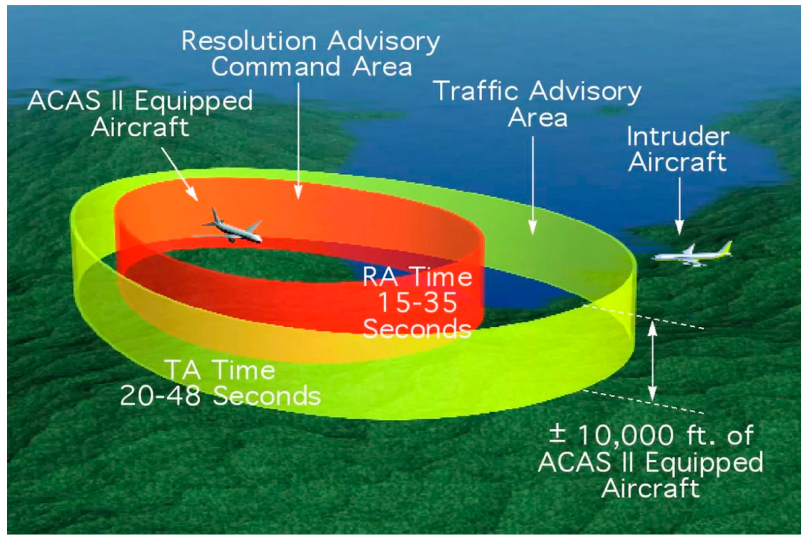
Moreover, as there is no clear collision avoidance standard for drones at present, we have assumed a reasonable collision judgment standard in the above scenario based on the existing standard. Currently, the collision avoidance system TCAS [35], used in civil aviation, mainly divides the airspace around an aircraft into “Traffic Advisory, TA”, and “Resolution Advisory, RA”, as shown in Figure 2. In the field of UAS, most of the literature and regulations emphasize the responsibilities of drone collision avoidance [36] or define the desired collision avoidance state of UTM [37], but do not elaborate on specific standards. In this paper, based on the performance of some actual logistics drones [38,39,40], we assume that a collision occurs between the drone and non-cooperative targets if the distance between them is less than 10 m.

3.2. Model Construction

Let  X  be the state space. Then denote  x 0 X  and  x f X  as the previous 4D waypoint and the next 4D waypoint, respectively. Assume that there are  n 1  static obstacles and  n 2  non-cooperative targets. Let  X i = 1 , , n 1 1 X  and  X i = 1 , , n 2 2 X  be the center of the  i th static obstacle and non-cooperative target, respectively. Then, the tactical conflict resolution problem can be described as follows:
min J ( u ) = J 1 + J 2
s.t.
x k + 1 = f ( x k , u k , k )
𝕊 = x t 0 = x 0 ,   x t f = x f ,
where  f ( )  is the state equation, whose specific explanation can be found in Equation (5);  x t 0  represents the initial state of the drone at the time of departure;  x t f  represents the final state of the drone at the time of mission completion; and  J 1  and  J 2  are the hazard cost function and the temporal difference cost function, respectively, which can be calculated as
J 1 = t = t 0 t f i = 0 n 1 R 1 ( x t , X i 1 ) + t = t 0 t f i = 0 n 2 R 2 ( x t , X i 2 ) J 2 = ( t f t ) 2 ,
where  t f  represents the estimated time of arrival of the drone at the next waypoint in the present situation;  t  represents the specific time of arrival pre-defined in the 4D trajectory planning;  R 1  represents the risk of the drone colliding with a static obstacle  X i 1  at time  t ; and  R 2  represents the risk of the drone colliding with the non-cooperative target  X i 2  at time  t . As can be seen from the above formula,  J 2  is a function that evaluates the difference between the estimated time of arrival of the drone at the next 4D waypoint and the specified time, with a smaller value indicating a smaller difference.
During the cruise stage, civil aviation drones generally fly in a fixed altitude layer [41]. Thus, in this study, we only consider the tactical conflict resolution of drones avoiding collisions with non-cooperative targets within the same altitude layer; that is, no changes in vertical altitude are considered. If a drone needs to avoid a collision, it can change its heading and speed by adjusting the speed of each rotor. Thus, the discrete state equation of the drone  x k + 1 = f ( x k , u k , k )  can be described as follows:
v k + 1 = v k + a k T x k + 1 = x k + v k T cos θ k y k + 1 = y k + v k T sin θ k θ k + 1 = θ k + ω k T ,
where  v k 0.1 , 10   m / s  represents the flight speed of the drone at time  k a k [ 3 , + 3 ]   m / s 2  represents the acceleration of the drone at time  k θ k  represents the yaw angle of the drone relative to the  x -axis at time  k ω k π / 30 , π / 30   r a d / s  represents the yaw angular velocity of the drone; and  x k  and  y k  are the drone’s horizontal and vertical coordinates in the Cartesian coordinate system at time  k , respectively.
By combining Equations (1)–(3) and (5), the problem studied in this paper can be defined as a discrete-time optimal control problem (DOCP), which involves determining a series of control factors  a k : t 0 , t f [ 3 , + 3 ]  and  ω k : t 0 , t f [ π / 30 , π / 30 ]  that minimize the performance indicator  J ( u )  while satisfying the objective set  S  and state equation  f ( )  at the same time.

4. Review of Typical Methods

4.1. Markov Decision Process and Reinforcement Learning

A Markov decision process (MDP) is a memory-less random control process in discrete time. Ronald A. Howard first improved the theoretical basis of the Markov decision process. Since then, MDP has been widely used in the fields of industrial automation, robotics, and artificial intelligence. A Markov decision process can be defined as a four-tuple  ( S , A , P , R ) , where S is a set of state sets and A is a set of action sets. The number of elements in these two sets can be finite or infinite; however, in general scenarios, the state and action sets with infinite numbers of elements are typically simplified to finite state and action sets. P is a probability density function,  P a s t , s = P s t + 1 = s s t = s , a t = a ,  providing the probability of state  s t ( s t S )  at time t, transferring to state  s t + 1 ( s t + 1 S ) at time t + 1 under action  a t ( a t A ). Finally, R is a reward function,  R a s t , s t + 1 , providing the reward value obtained after state  s t  is transferred to state  s t + 1  under the action  a t . The action  a  at any moment is provided by the strategy function  π a s = P A = a S = s  for a given state  s . The optimization goal of MDP is to determine the optimal strategy function  π *  through some method, thus achieving the maximum reward expectation of the system.
Reinforcement learning is an interactive learning method based on MDP. The related concept of reinforcement learning was first proposed by Minsky [42], and then refined by Bellman, Watkins, and others. The mechanism of reinforcement learning is similar to that of human reward and punishment, guiding learning through behavioral judgment.
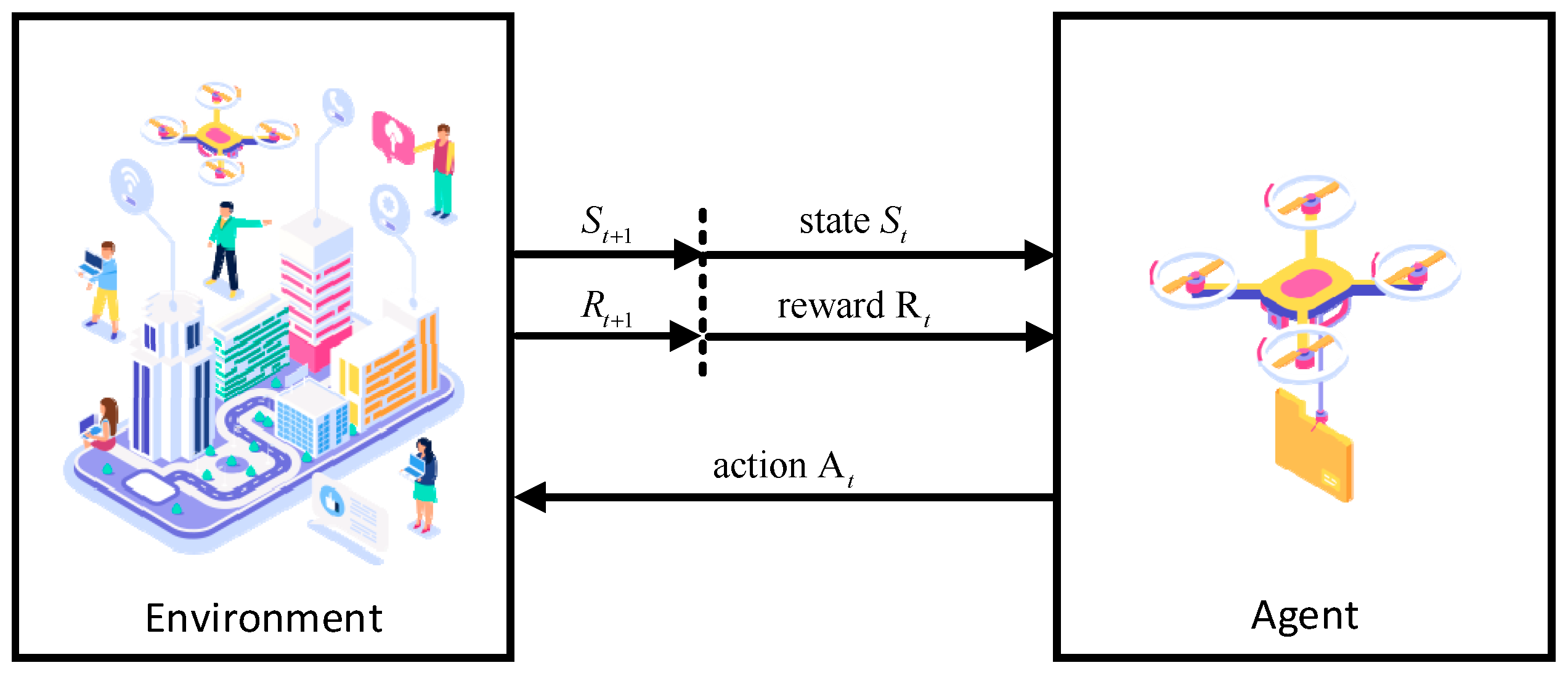
Based on MDP, reinforcement learning introduces the concepts of agent and environment, where the subject carrying out an action is referred to as an agent, and the entity that interacts with the agent is called the environment. Figure 3 shows a basic block diagram of reinforcement learning.
Specifically, in each interaction between the agent and environment, and following the pre-designed rules, the agent perceives a state of the environment, then selects and executes an action based on that state. After the agent completes an action, the environment will return a reward based on the new state achieved, indicating the quality of the action selected by the agent. Then, the agent determines the action plan that achieves the maximum reward by performing numerous explorations (i.e., trials and errors) in the environment.

4.2. Introduction of the D3QN Algorithm

4.2.1. Deep Q-Networks

The Deep Q-Network (DQN) is a deep reinforcement learning algorithm proposed by the DeepMind team [43]. By replacing the Q-table with a neural network, DQN resolves the “Curse of Dimensionality” problem encountered by the Q-learning algorithm when considering a continuous state space. In order to achieve a maximum accumulated reward in a task, the agent selects actions based on the states in the environment with the following optimal action–value function  Q * ( s , a ) :
Q * ( s , a ) = max π E   [ r t + γ r t + 1 + γ 2 r t + 2 + | s t = s , a t = a , π ] ,
where the  γ  represents the attenuation factor and  r t  refers to the reward at time step  t  that an agent can obtain after taking action  a  in the state  s  by the optimal strategy  π = P ( a | s ) .
Additionally, the experience replay method, as well as the target network, ensure the convergence of the model and the stability of training. The experience replay usually stores the experience sample  ( s t , a t , r t , s t + 1 )  of the agent at each time step  t  in the experience pool  D . During the learning process, experience samples  ( s , a , r , s ) ~ U ( D )  are randomly selected for network updating. After introducing the target network, the update loss function for the  i th iteration  L i ( w i )    is as follows:
L i ( w i )   =   E ( s , a , r , s ) ~ U ( D ) r + γ m a x a Q ( s , a ; w t ) Q ( s , a ; w e ) 2 ,
where  w e  and  w t  represent the parameters of the main and target networks, respectively, and  m a x a  is the maximum value. After each step  C , the parameters of the main network are updated, along with those of the target network.

4.2.2. Double DQN

In DQN, actions are selected and evaluated using the same networks, potentially leading to over-estimation, which is detrimental to model learning. To solve the over-estimation problem, Van Hasselt H. et al. [44] proposed a Double DQN algorithm, in which two structurally identical neural networks are used as the current and target networks. The current network is responsible for selecting actions, while the target network calculates error targets. By separating the action selection from value estimation, the algorithm mitigates the over-estimation of Q-values that can occur in the DQN algorithm when selecting the maximum Q-value for action execution, which could adversely affect the original network. The objective function used in Double Q-learning is:
Q t r t + 1 + γ Q ( S t + 1 , arg max a Q ( S t + 1 , a ; w e ) ; w t )   ( Double   Q-learning ) ,
where the parameter  w e  is used for action selection and the parameter  w t  is used for action evaluation.

4.2.3. Dueling DQN

For faster and better training results, Wang et al. [45] introduced a new neural network architecture that decouples the value function  V * s t  and advantage function  A * s t , a t  in DQN while sharing a common feature learning module. This function can evaluate the quality of each action while predicting the value function, allowing the state value function to be learned more frequently and accurately. The formula for each network output of Dueling DQN is as follows, where  w  represents the network parameters:
Q ( s , a ; w , α , β ) = V ( s ; w , β ) + A ( s , a ; w , α ) 1 | A | a A ( s , a ; w , α ) .
The optimal value function of the Dueling DQN algorithm is as follows:
Q t = r t + 1 + γ max α Q s t + 1 , a ; w t ,
where  w t  represents the parameters of TargetNet. With the TargetNet, all action values in the state can be obtained, following which a target value can be calculated based on the optimal action value.

4.2.4. Dueling Double DQN

The Dueling Double DQN (D3QN) algorithm was created by incorporating the ideas of the Double DQN algorithm into the Dueling DQN algorithm. The only difference between the D3QN algorithm and the Dueling DQN algorithm is how the target value is calculated. Applying the target network and evaluation network in Equation (11) (Dueling) separately, we can obtain the optimal value function of the D3QN algorithm as follows:
Q t = r t + 1 + γ Q s t + 1 , a r g m a x a Q s t + 1 , a ; w e ; w t ,
where  w e  represents the parameters of MainNet and  w t  represents the parameters of TargetNet. In this way, the action corresponding to the optimal action value under the state can be obtained with the MainNet, while the obtained action’s value under the state can be calculated to find the target value using the TargetNet, thus mitigating the over-estimation problem.

5. Method

5.1. Environment Construction for the Problem

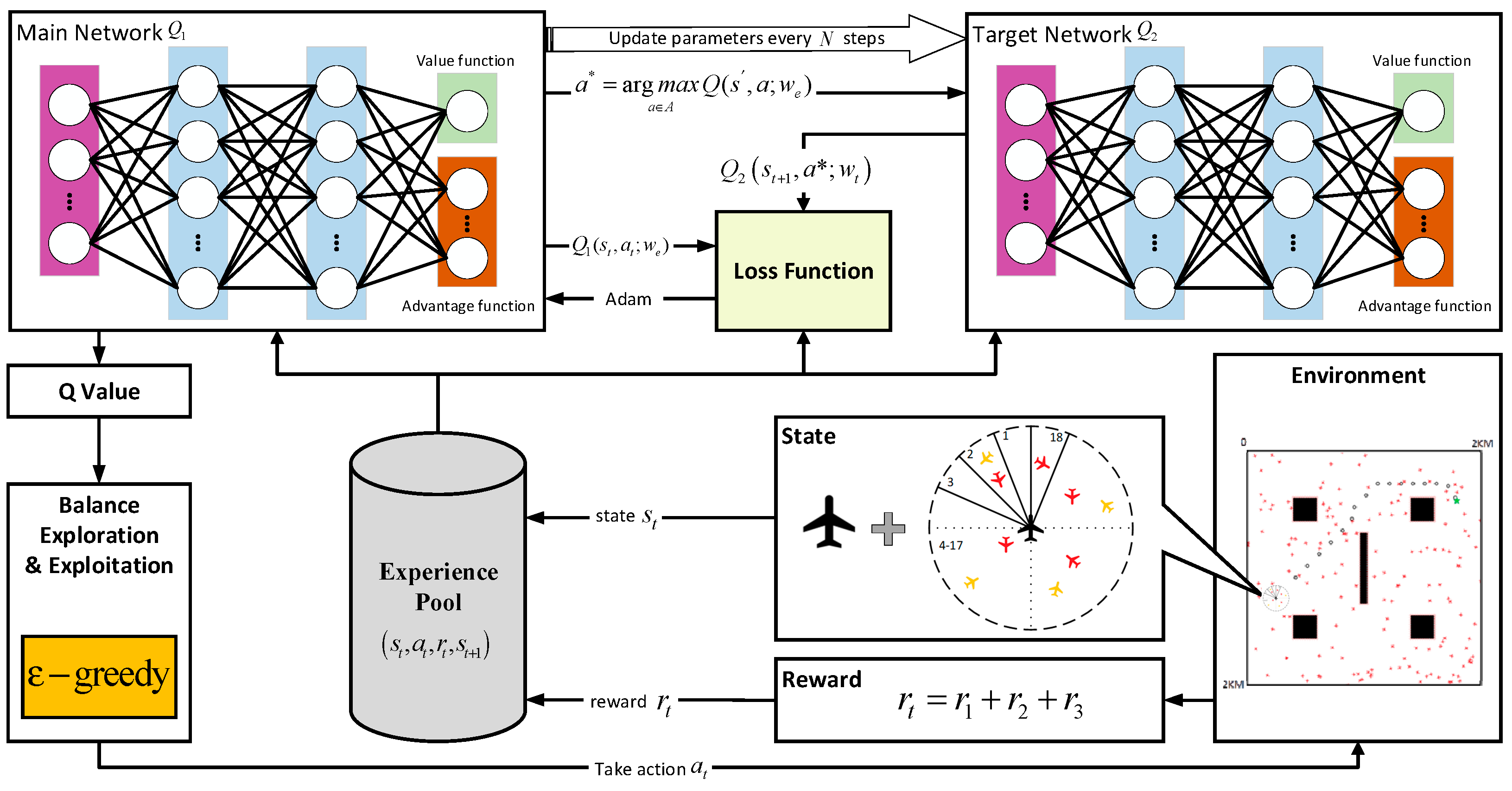
The maneuvering of a drone in flight to avoid collisions with non-cooperative targets can be viewed as a sequential decision optimization problem, which can be represented as a series of MDP. In this paper, the tactical conflict resolution problem under the temporal constraints of a strategic 4D trajectory is solved using the Dueling Double DQN algorithm with a novel state space description and an ETA-based reward. The integrated framework of this solution is depicted in Figure 4.

5.1.1. State Space

The state space is a subset of the agent’s observations of the environment, and we assume that the drone under control can accurately perceive its surrounding environment, including non-cooperative targets. Unlike the commonly researched consumer-grade drones, logistics drones require a higher level of safety standards and must comply with specific unmanned aircraft operational regulations [46]. Based on a literature review conducted earlier, existing methods have limitations regarding the number of targets they can avoid simultaneously, such that the success rate of these methods is heavily influenced by the number of non-cooperative targets. Therefore, they have not yet met the standards mentioned above. To improve the probability of success rates, the novel concept of risk sectors is introduced in this paper to reconstruct the state space, allowing for the position and distance of a non-cooperative target to be expressed simultaneously.
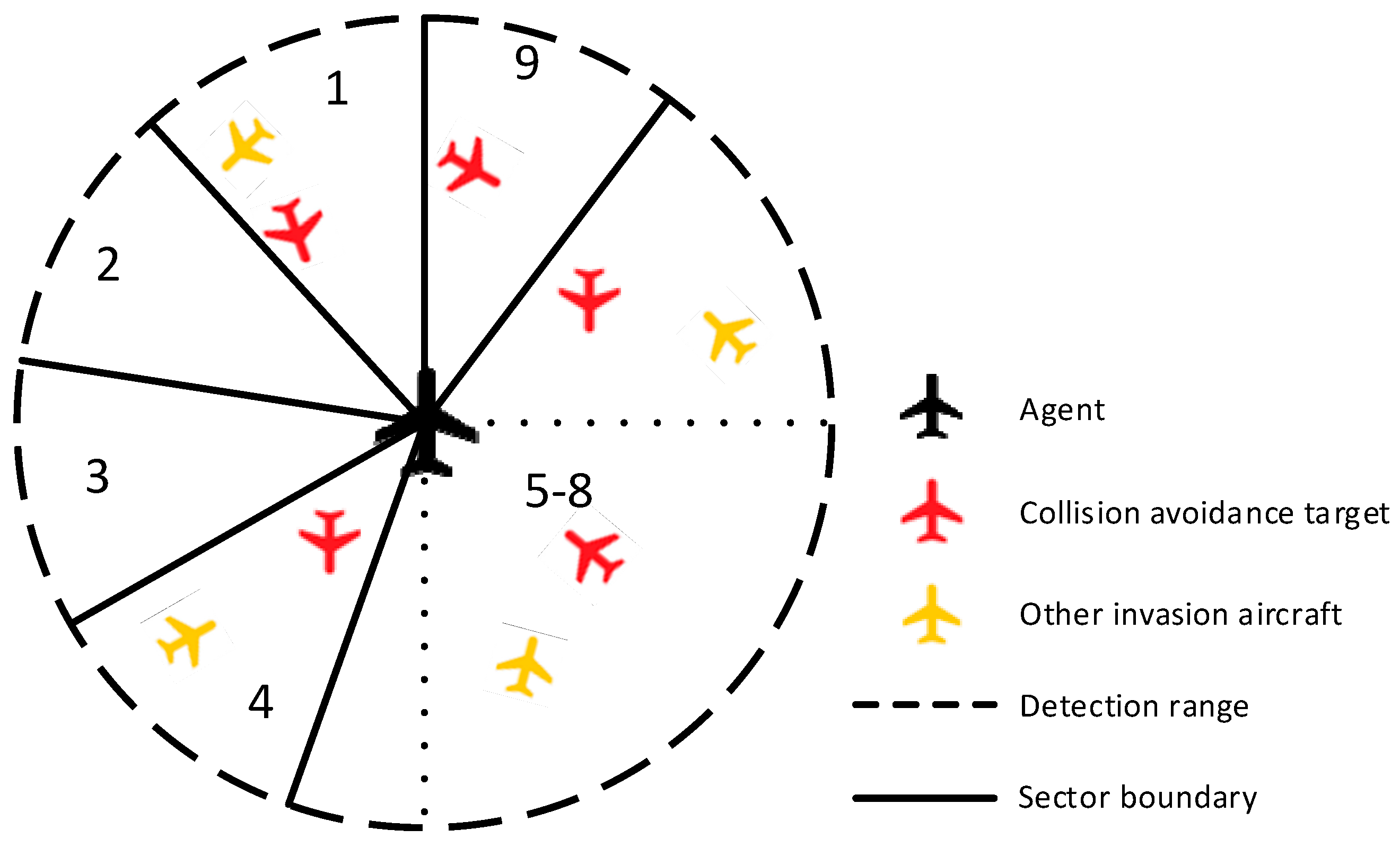
To achieve collision avoidance with an indefinite quantity of non-cooperative targets simultaneously using the deep reinforcement learning method, we first divide the detection range into N sectors and consider only the nearest non-cooperative target in each sector, as shown in Figure 5. If there are multiple threatening non-cooperative targets in a sector, their directions relative to the aircraft are limited to that sector, which can be assumed to be the same. Therefore, the non-cooperative target closest to the aircraft can describe the threat of the non-cooperative targets in that sector clearly, so, considering only the nearest non-cooperative target in each sector is reasonable.
The main purpose of this method is the reconstruction of the state space based on sectors, which provides implicit directional information for the neural networks while also reducing and fixing the dimension of the state space. This allows the relative distance, relative angle, and other threat information of non-cooperative targets in the same sector to be described using only the one-dimensional information of the relative distance to the nearest threatening target in that sector.
For instance, in Figure 5, there are nine non-cooperative targets within the detection range. With traditional methods, describing them requires at least two-dimensional information, including the relative angle and relative distance, resulting in a state space dimension of 18. In contrast, our method divides the detection space into nine sectors and uses the relative distance to the nearest threatening target in each sector as the state space, resulting in a fixed state space dimension of nine. As a result, this state space is much smaller than that in traditional methods and is not affected by the number of non-cooperative targets within the detection range, thus increasing the convergence ability and speed of neural network training.
In this paper, it is assumed that the detection range of a drone is a circle with the drone’s geometric center as its center and a radius of 100 m, and that the drone can obtain the information for all non-cooperative targets within this range. Specifically, considering the pre-defined four-dimensional waypoint constraints at the strategic level, the state space  S  at time  k  in this paper consists of three parts expressed as:
S k = [ S k 1 , S k 2 , S k 3 ]
where  S k 1 S k 2 , and  S k 3 , respectively, represent the status information of the drone itself, the pre-defined strategic trajectory temporal information, and the threat status information of the nearest target in each sector. In addition,  θ k  and  v k  denote the heading angle and the velocity of the drone at time  k , respectively. If the drone is currently between waypoint  n  and waypoint  n + 1 , we use  t e t a  to denote the estimated time of arrival (ETA) when the drone arrives at waypoint  n + 1 t n o w  to denote the current coordinated universal time, and  t n n + 1  to represent the temporal difference between the pre-defined time of arrival at waypoints n and n + 1 in the pre-determined 4D trajectory. If  d 1  and  d 2  denote the distance between the current position of the drone and waypoint  n + 1  and the distance between waypoints  n  and  n + 1 , respectively, as shown in Figure 6, then,  S k 1  and  S k 2  can be expressed as
S k 1 = [ θ k , v k ]
S k 2 = [ p k d , ψ k , p k t ] ,
where  p k d = d 1 / d 2  represents the normalized remaining distance between the current position of the drone and waypoint  n + 1 ψ k  represents the angle required for the drone to turn counterclockwise to face waypoint  n + 1  at time 𝑘, and  p k t = ( t e t a t n o w ) / t n n + 1  represents the normalized remaining time for the drone to reach waypoint  n + 1 .
The elements in  S k 3  represent the normalized relative distances between the current position of the drone and the non-cooperative targets. The position of the closest non-cooperative target in the  n th sector is denoted by  D n , and the state space is filled with a 1 if there is no threatening target in a certain sector. Then,  S k 3  can be represented as
S k 3 = [ D 1 , D 2 , D 3 , , D n ] .

5.1.2. Action Space

The algorithm selects an action for each subsequent state, starting from the initial moment. In each action, the drone’s yaw angle, acceleration, or both are controlled based on certain values. Based on the performance of some actual logistics drones [38,39,40], the action space consists of the left and right yaw and level flight, with yaw angle velocities in the range of  [ π / 30 , 0 , + π / 30 ]   r a d / s  and accelerations in the range of  3,0 , + 3   m / s 2 . Meanwhile, the final speed of the drone is limited to the range of 0.1–10 m/s. Once a new state is reached, the algorithm selects an appropriate yaw angle velocity and acceleration, based on the current state, in order to control the drone and maintain the current action until a new action is selected or the final state is reached. The discretized action space is described in Table 1.

5.1.3. Reward Function

The reward value is the only feedback a drone can receive from the environment and is used to evaluate the goodness or poorness of a selected action under the current state. For the problem described in Section 3, two objectives should be considered: 1. the drone should be able to safely avoid collision with any non-cooperative target or static obstacle, and 2. the drone should arrive at the next 4D waypoint at a specific time to minimize secondary conflicts. To accomplish these objectives, a collision avoidance reward and an ETA-based reward are introduced. Specifically, the collision avoidance reward  R 1  was designed to assess the safety performance of the drone at the current moment first. Meanwhile, the correlation between strategic-level trajectory planning and tactical-level conflict resolution is considered for the first time by introducing the estimated time of arrival. In this way, an ETA-based temporal reward was designed to provide non-sparse rewards for drones whose estimated time of arrival is not within the specified time window. Finally, a mixture of sparse and non-sparse rewards was designed to encourage drones to reach their next waypoint in a timely manner. The details of these rewards are discussed in the following.
(1) Collision avoidance reward  R 1
The comprehensive collision avoidance reward value  R 1 , which can be obtained in each time step, is calculated as follows:
R 1 = R u 1 + R u 2 ,
where  R u 1 = r u 1 + r u 2  is a non-sparse reward, designed to cope with the avoidance of non-cooperative targets (if any) within the drone detection range. Then,  r u 1  is defined as follows:
r u 1 = c 1 , i f             D k i D k 1 i 0 c 1 , i f             D k i D k 1 i < 0 ,
where the reward  c 1  or penalty  c 1  is based on the relative motion trends of the drone and non-cooperative targets in each sector;  D k i  and  D k 1 i  represent the distance between the drone and the closest non-cooperative target in sector  i  at time  k  and  k 1 , respectively; and  r u 2  is the penalty, which is based on the normalized distance of the closest non-cooperative target in each sector:
r u 2 = ( 1 D k i 100 ) α r 1 ,
where  α r 1  represents the danger penalty coefficient.
Meanwhile,  R u 2  is set to penalize collisions and can be denoted as
R u 2 = c 2 , D k i s j { D k i s j , D k i s j < c 3 } 2 c 2 , D k i { D k i , D k i < c 3 } ,
where  c 2  is the collision penalty value to stimulate drones to avoid non-cooperative targets and static obstacles,  c 3  is a collision threshold, and  D k i s j  represents the distance between the drone and static obstacle  s j .
(2) Temporal Reward  R 2
To meet the temporal constraints of the strategic 4D trajectory, by introducing the ETA of the next waypoint, an ETA-based temporal reward  R 2  is proposed in this paper which can be represented as
R 2 = r e + r l ,
where  r e  and  r l  are the early arrival penalty and late arrival penalty, respectively, and are defined as follows:
r e = ( p k t p k d ) α r 2 1 t r α r 2 2 0 ,   t r   >   0 ,   t r   <   0 ,
r l = ( p k t p k d ) α r 2 3 + t r α r 2 4 0 ,   t r   <   0 ,   t r   >   0 ,
where  t r    represents the time difference of arrival at the next waypoint between the pre-defined 4D trajectory and the current situation, defined as follows:
t r = t n + 1 t e t a ,
where  t e t a  can be calculated as
t e t a = t now + d 1 V .
In the above equation,  V  is the weighted velocity, which changes as the current state changes:
V = V = α v ( V a + V min ) V = α v ( V a + V max ) , , p k t > p k d + d t p k t + d < p k d ,
where  p k t  and  p k d  denote the normalized remaining time and the normalized remaining distance, respectively; and  d t  is the time window threshold.
As defined above, when the normalized remaining time  p k t  for the drone to reach the next waypoint is greater than the sum of the time window threshold  d t  and the normalized remaining distance  p k d , the drone exhibits an early arrival tendency. At this time, if the drone cannot arrive at the next waypoint on time while flying at the slowest speed ( V min ), an “early arrival” will inevitably occur and an early arrival penalty  r e  should be added to the drone. Vice versa, if the sum of the time window threshold  d t  and normalized remaining time  p k t  for the drone to reach the next waypoint is less than the normalized remaining distance  p k d , the drone exhibits a late arrival tendency. At this time, if the drone cannot arrive at the next waypoint on time while flying at the fastest speed ( V max ), a “late arrival” will inevitably occur and a late arrival penalty  r l  should be added to the drone.
(3) Mission reward  R 3
The final reward  R 3  is set to stimulate the drone to reach the geographic coordinates of the next 4D waypoint and can be expressed as follows:
R 3 = R g 1 + R g 2 ,
where  R g 1 = k 3 0  is a sparse reward, which is added when the geographic coordinates of the next 4D trajectory point are reached. Meanwhile,  R g 2 = r 3 1 + r 3 2  is a safety-first non-sparse mission reward that can be divided into two parts: the line-of-sight reward  r 3 1  and the destination distance reward  r 3 2 . In this regard,  r 3 1  is set to adjust the heading angle to fly to the next 4D waypoint, and can be represented as
r 3 1 = c 4 , ψ k 0 , π 18   35 18 π , 2 π and m = 0 c 5 , ψ k π 18 , 2 18 π 34 18 π , 35 18 π and m = 0 0 , ψ k 9 18 π , 27 18 π and m = 0 or m > 0 c 6 , ψ k 2 18 π , 9 18 π 27 18 π , 34 18 π and m = 0 ,
where  m  represents the number of non-cooperative targets within the detection range,  c 4  and  c 5  are the corresponding reward values,  c 6  is the penalty value for the situation that the next 4D trajectory point is in the opposite direction, and  r 3 2  is set to guide the drone to fly toward the next 4D waypoint, which can be represented as
r 3 2 = α r 3 1 ( d 1 k 1 d 1 k ) , m = 0 α r 3 2 D min k 1 D min k , m > 0 and D min k 1 D min k c 7 , m > 0 and D min k 1 < D min k ,
where  d 1 k 1  and  d 1 k  are the distance between the drone and the next waypoint at time  k 1  and  k , respectively;  D min k 1  and  D min k  are the minimum distances between the drone and the nearest non-cooperative target within detection range at times  k 1  and  k , respectively;  c 7  is the corresponding penalty value; and  α r 3 1  and  α r 3 2  are the reward coefficients.
Following the rewards set above, on the one hand, if any non-cooperative target is detected within the detection range, the drone will be guided to avoid any collision first, in order to ensure that safety is maintained, and then to the next 4D waypoint. On the other hand, if no target is detected within the detection range, the drone will be guided to the next 4D waypoint immediately.
As a result, by adding the rewards mentioned in Equations (16), (20) and (26), the final comprehensive reward that the drone can achieve after executing each action can be calculated  R = R 1 + R 2 + R 3 .

5.2. Algorithm

In practice, the greedy search strategy, delayed learning strategy, and multi-step learning have been introduced in the baseline D3QN algorithm to improve its robustness and results. According to the above developments, the D3QN with a reconstructed state space and a novel ETA-based reward is described in Algorithm 1. Lines 6–9 in the code are used to randomly select an action based on the greedy search strategy. In Line 12, a new state  s t + 1  is observed from the environment after the drone has executed the optimal action  a t . Then, in Lines 13–15, the collision avoidance reward  R 1 , final temporal reward  R 2 , and comprehensive mission reward  R 3  are obtained by Equations (20), (26) and (35), respectively.  E s  Line 18 represents the status of the episode (i.e., ended or not). In Line 18, the experience fragments  ( s t , a t , r t , s t + 1 , E s )  of the agent are stored in the experience pool. Finally, in Line 21, the Q-value is updated by using Equation (20).
Algorithm 1 Pseudocode of D3QN in this paper
1 Create a training environment
2 Initialize the network parameters and experience pool
3 for episode = 1 to M do
4 Initializing the Environment S
5 for t = 1 to T do
6    if random > ε then
7    pick an action at random
8    else
9    action  a t = max a Q ( s t + 1 , a ; w e )
10   end
11   execute the action  a t  
12   get  s t + 1 = e n v . O b s e r v a t i o n ( s t , a t )
13   get  R 1 = e n v . r e w a r d _ 1 ( s t , a t )
14   get  R 2 = e n v . r e w a r d _ 2 ( s t , a t )
15   get  R 3 = e n v . r e w a r d _ 3 ( s t , a t )
16    r t = R 1 + R 2 + R 3
17    E s = e n v . s t e p ( s t , a t )
18   store fragments  ( s t , a t , r t , s t + 1 , E s )  in the experience pool
19   if the current round is a training round then
20   randomly extract fragments  ( s t , a t , r t , s t + 1 , E s )  from the experience pool
21    update the Q-value
       Q ( s t , a t ) Q ( s t , a t ) + α ( R t + 1 + γ Q ( S t + 1 , arg max a Q ( S t + 1 , a ; w e ) ; w t ) Q ( s , a ; w e ) )
22    end
23    if the current round is the updated target network round then
24    copy the parameters  θ  of the current network to the target network
25    end
26    if  E s  is ended then
27    break
28 end

6. Simulation

6.1. Platform

6.1.1. Simulation Scene Setting

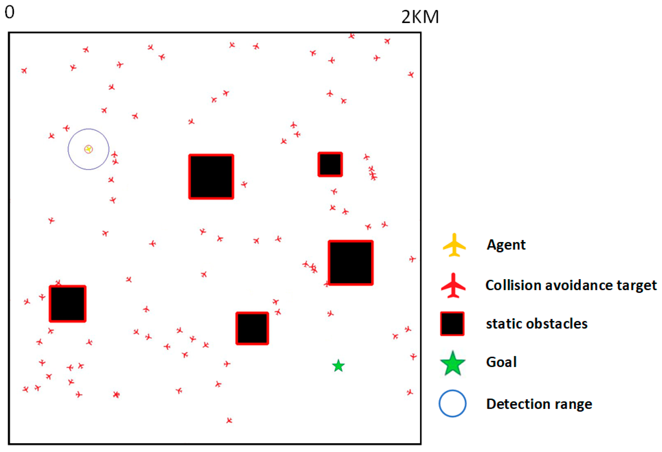
In this section, we consider a two-dimensional plane environment to demonstrate the superiority of our proposed method. Following the altitude division mentioned in the previous section, for the experimental scenario, we selected a true altitude of 120 m as the cruising altitude of the drone, and only the horizontal movement of the drone was considered at this altitude layer. The airspace includes the drone, non-cooperative targets, target points, and five static obstacles. The positions and sizes of the obstacles were randomly generated and independent of each other. The training airspace was a 2 km × 2 km area, gridded according to pixel points, where each pixel represents a square area of 2 m in length and width (as shown in Figure 7).
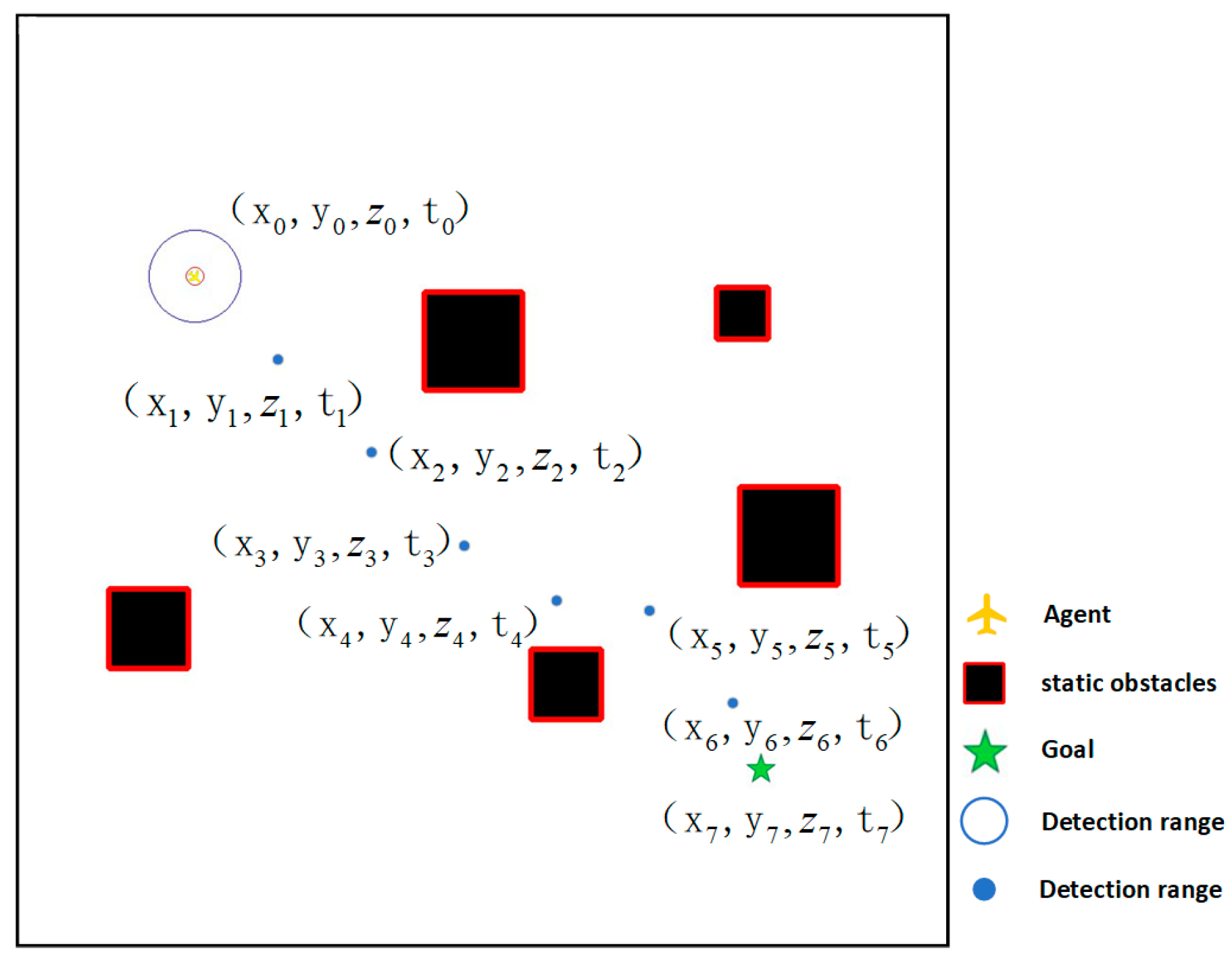
Following the standard specification for UTM and USS interoperability, the A* algorithm was used in the strategic trajectory planning phase to obtain a series of pre-determined 4D waypoints. Specifically, every 100 m along the path, a path point was selected. The time dimension simulation was conducted based on the distance between path points, planned cruising speed, and buffer time, in order to estimate the expected time to reach the next path point. The buffer time was determined according to the distance of the entire route and the elasticity time coefficient. The planned path, consisting of a series of 4D waypoints, is shown in Figure 8.

6.1.2. Reinforcement Learning Setting

The training process and structure of a deep reinforcement learning algorithm are largely influenced by the hyper-parameter settings. In order to remove the influence of the hyper-parameter settings on the training results, uniform settings were applied to the common parameters used by the algorithm. Following [47,48,49], the specific parameters of D3QN are listed in Table 2 below.
All the guidelines and tests discussed in this paper were completed in a Win10 system with unified software and hardware environment information. The CPU was an Intel(R) Xeon(R) W-2133, the motherboard was an Intel 440BX Desktop Reference Platform, and the GPU was an NVIDIA GeForce RTX 2080 Ti.
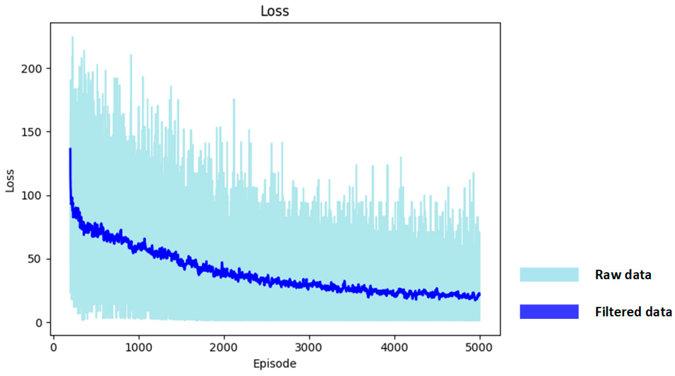
During the training process, the loss function and reward values per round are important indicators that reflect the convergence and performance of a deep reinforcement learning algorithm. In this study, the basic conflict resolution ability of the drone was pre-trained in a scenario with 40 non-cooperative targets in a 1 square kilometer area. The loss error values are shown in Figure 9.
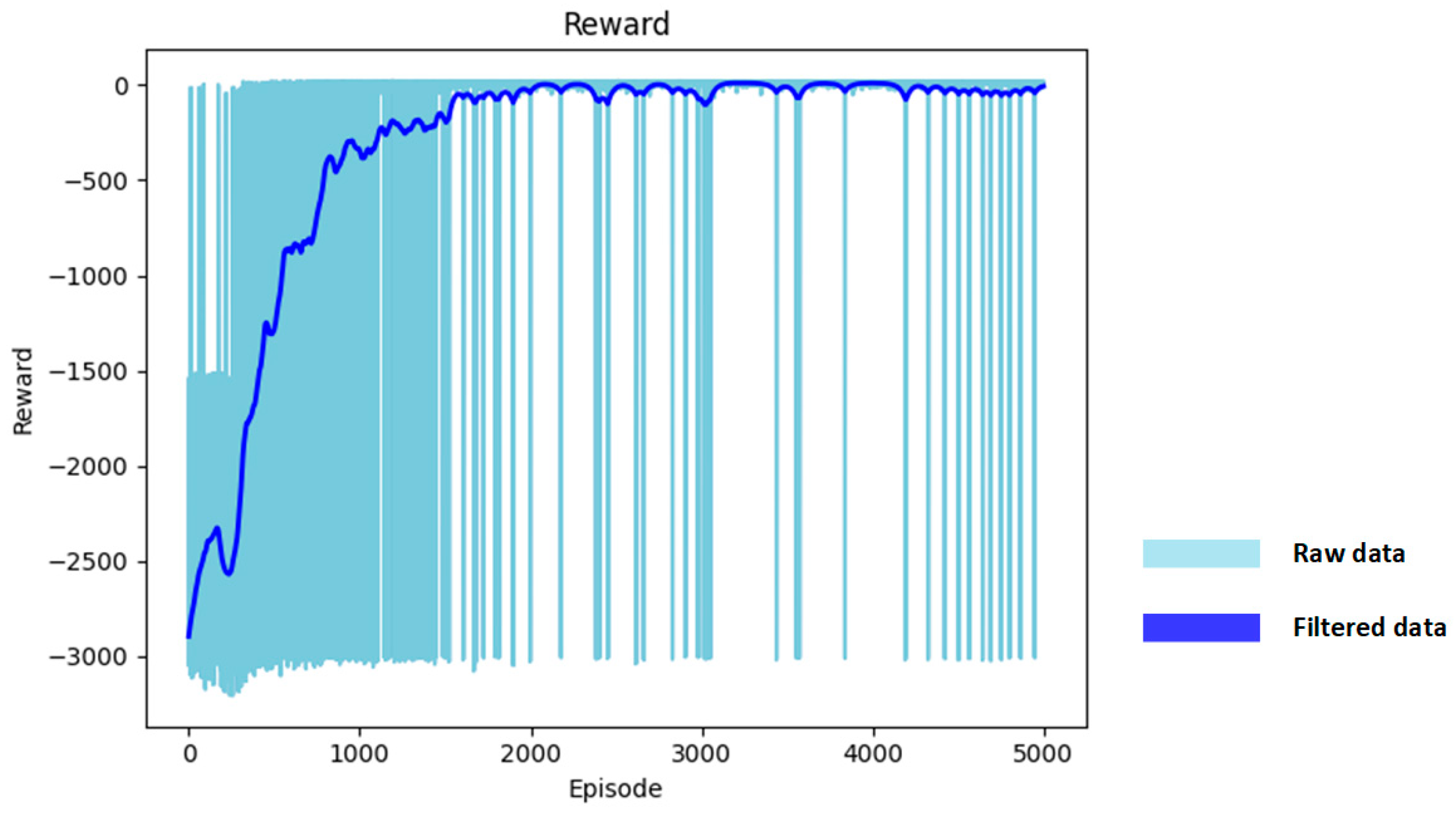
The figure shows that, as the number of training iterations increased, the loss error gradually decreased and stabilized, indicating that the algorithm had converged and learned a fixed strategy. The reward values for 5000 rounds of the algorithm are shown in Figure 10.
The figure shows that the average reward value of the drone constantly increased in the first 0–1500 iterations, indicating that the drone was continuously learning and optimizing its strategy. From 1500 to 5000 iterations, it can be observed that the average reward value gradually stabilized and approached the maximum value, indicating that a stable conflict resolution strategy had been formed.

6.2. Test 1: Comparison Analysis of Sector Improvement

6.2.1. Task Setting

The main objective of this experiment was to verify whether the method proposed in this paper for reconstructing the state space using the risk sector concept can improve the tactical conflict resolution success rate of an unmanned aerial vehicle (UAV). Based on the logistic UAV operating density obtained in Phase Two of NASA’s UTM Pilot Program (UPP), which is 14.57 UAVs per square kilometer [3], we set the number of non-cooperative targets in the above experimental scenario to 15 per square kilometer. In UAV conflict resolution using reinforcement learning, the state space usually consists of information such as distance, position, and velocity [50]. Therefore, for this experiment, we set up two state spaces for training and testing. The state space of experimental group 1, which consists of both the onboard information and the risk sectors constructed in Section 5.1.1, can be expressed as:
[ θ k , v k , p k d , ψ k , p k t , D 1 , , D 9 ] .
Experimental group 2 followed a commonly used method for the construction of the state space, where the first part was the same as that of experimental group 1, which records the information of the host aircraft. The second part records the normalized distance and bearing information of the nine closest non-cooperative targets and obstacles, which can be expressed as:
[ θ k , v k , p k d , ψ k , p k t , d i s t 1 , ψ 1 , D 2 , ψ 2 , D 9 , ψ 9 ] ,
where  ψ i , i = 1,2 , 3 , 9  represents the angle (in degrees) at which the unmanned aerial vehicle’s heading should be rotated counterclockwise to face the ith nearest non-cooperative target or obstacle.

6.2.2. Simulation Results

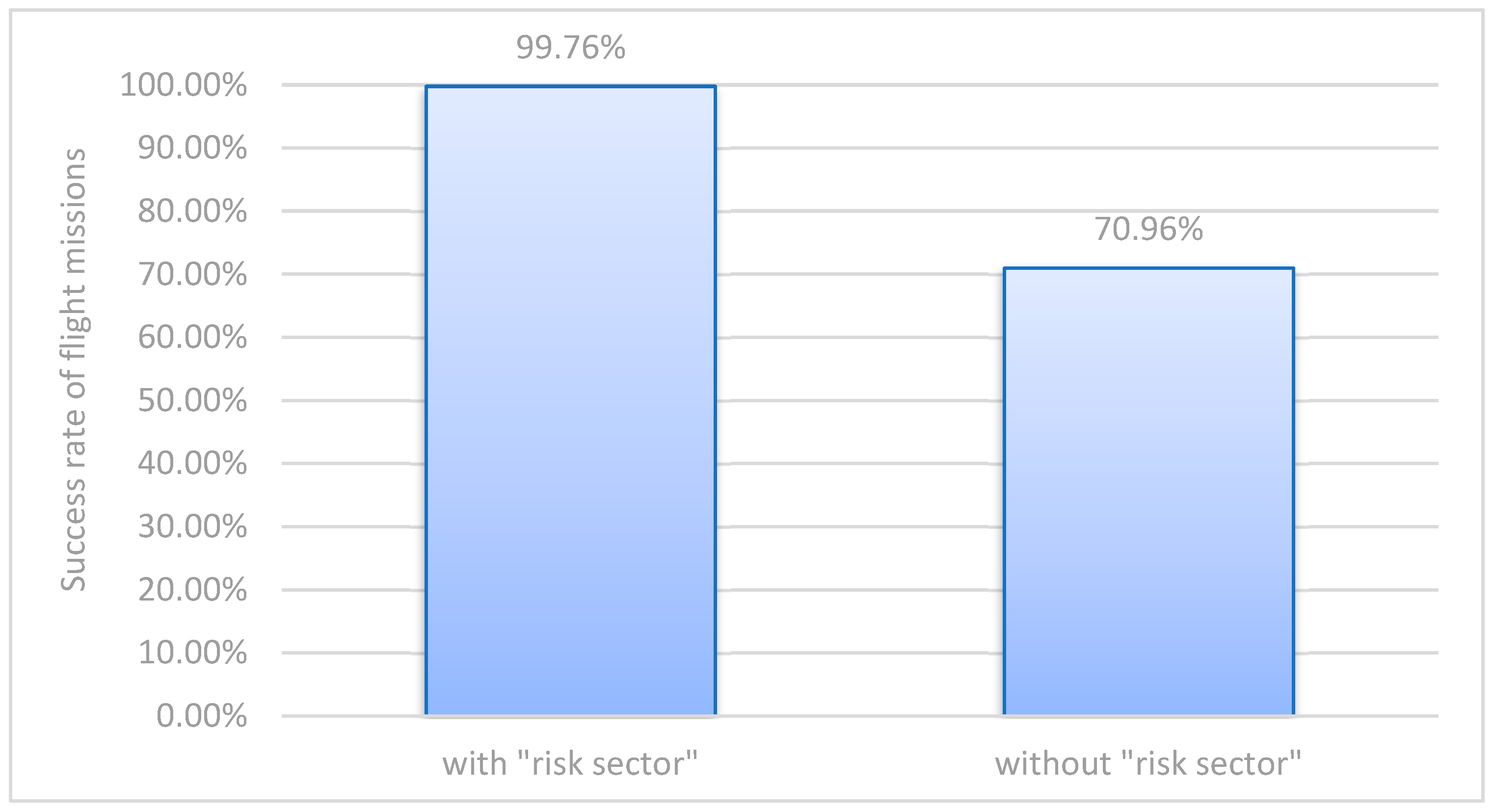
After training both experimental groups, the strategy for tactical conflict resolution with the highest success rate of flight missions was selected for each group and tested 10,000 times under the same parameters; the “Success rate of flight missions” indicates the probability of the drone successfully flying from the starting point to the end point while avoiding non-cooperative targets. This metric does not consider whether the drone arrives at the end point on time or not. Based on the test results shown in Figure 11, it can be seen that the reconstructed state space significantly increased the success rate of flight missions, with an improvement of 40.59% compared to the general solution.

6.3. Test 2: Ablation Study of the ETA-Based Temporal Rewards

6.3.1. Task Setting

To demonstrate the effectiveness of our ETA-based temporal rewards proposed in Section 5, in the next experiment, we mainly trained and tested different temporal reward strategies in the scenario described earlier, using 15 non-cooperative targets per square kilometer. Four different reward settings for the early arrival penalty  r e  and late arrival penalty  r l  were considered, including: (1) without  r e  and  r l ; (2) with  r e ; (3) with  r l ; and (4) with  r e  and  r l .

6.3.2. Simulation Results

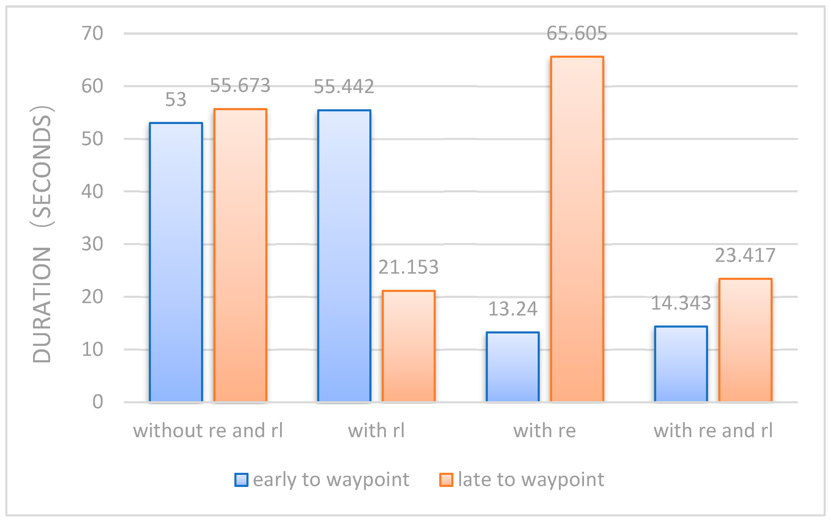
After training under the four reward settings, the conflict resolution strategy with the highest success rate was selected for 10,000 tests under the same parameters. From Figure 12 and Table 3, it can be seen that, after adding the late penalty  r l  to the drone, there was no significant change in early arrival compared to the reference group, but the duration of being late was reduced by 62%. After adding the early penalty  r e  to the group, although the duration of early arrival was reduced by 75.02%, the duration of being late increased by 17.84%. With the combined penalty (i.e.,  r e  and  r l ), the early and late arrival situations of the drones were both improved, with the duration of early arrival reduced by 72.94% and the duration of being late reduced by 57.94%, resulting in significant performance improvement. The reason why the effect of  r e  was more significant than that of  r l  may be that the subject of this study is a quadrotor that can perform a low-speed flight, while its maximum speed is limited. It is worth mentioning that the “on time rate” is influenced by the time window, i.e., only the drone reaching the 4D waypoint within the time window can be considered on time.
Furthermore, it is worth mentioning that, according to the experimental results given in Table 3, even after adding different temporal rewards to the conflict resolution strategy, the proposed approach can still maintain a very high success rate, with all being above 99%.

6.4. Test 3: Exploring the Maximum Density in the Scenario

6.4.1. Task Setting

The main purpose of this experiment was to verify whether the conflict resolution strategy proposed in this paper can achieve an equivalent level of safety flight capability as specified in the literature [51,52]; that is, “an accident rate lower than 0.2 per 10,000 flight hours”. For verifying this, under the condition of the same number of accidents per 10,000 h as TCASII, we found the maximum non-cooperative density of our method, which is 3.3 times higher than the original TCASII standard.
In this experiment, each pixel point was set to 20 m and the simulated scenario was expanded to 400 square kilometers. A total of 24 sets of non-cooperative target densities were set for 100,000 simulation tests, with 180,000 flight hours for each set.

6.4.2. Simulation Results

The experimental results shown in Figure 13 indicate that, in the scenario with a density of 0.2 aircraft per square kilometer, no collision accidents occurred during the 180,000 h of flight when using the strategy proposed in this paper. By observing the experimental data, it can be concluded that the density of non-cooperative targets in the airspace is linearly related to the number of accidents per 10,000 flight hours. After fitting the experimental data, it was calculated that when the accident rate per 10,000 flight hours is 0.2, as described above, the density of non-cooperative targets in the airspace is 0.89 aircraft per square kilometer which is 3.3 times higher than the TCAS II standard. It is worth mentioning that the blue line in Figure 13 is obtained by using the least square method and the expression is:  y = 0.95 x 0.063 .

6.5. Test 4: Case Study

6.5.1. Task Setting

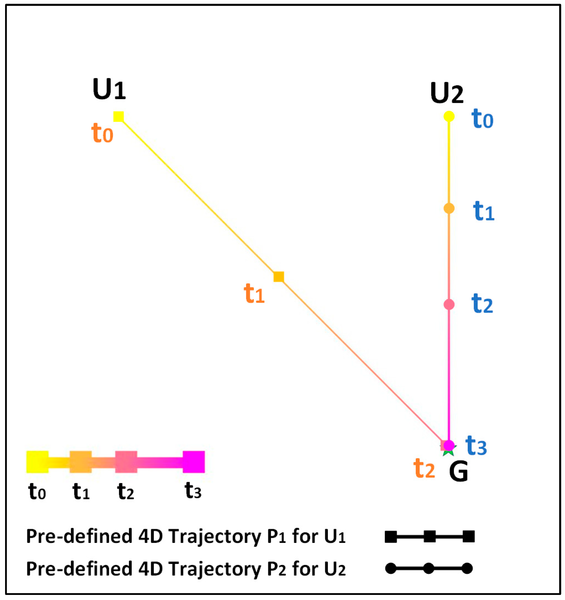
All of the cases detailed above demonstrate the superiority of our method from a macro perspective, such as its success rate. In this case study, we used a specific local scenario to illustrate the effectiveness of our method. Specifically, we compared the paths between two waypoints generated with and without our ETA-based temporal reward  R 2 . In this scenario, as shown in Figure 14, two drones  U 1  and  U 2  moved forward along the pre-planned 4D trajectories  P 1  and  P 2 , respectively, and arrived at the waypoint  G  at time  t 2  and  t 3 t 3  respectively. Obviously, there was no conflict between the two aircraft in the strategy path planning phase. However, after adding the non-cooperative targets into the scenario described above, the drones may fail to reach their next trajectory points on time while executing their tactical conflict resolution strategies, leading to secondary conflict. In the simulation, the non-cooperative target density was set to 15 per square kilometer, and we assumed that  U 2  can follow the pre-planned 4D trajectory  P 2  perfectly.

6.5.2. Simulation Results

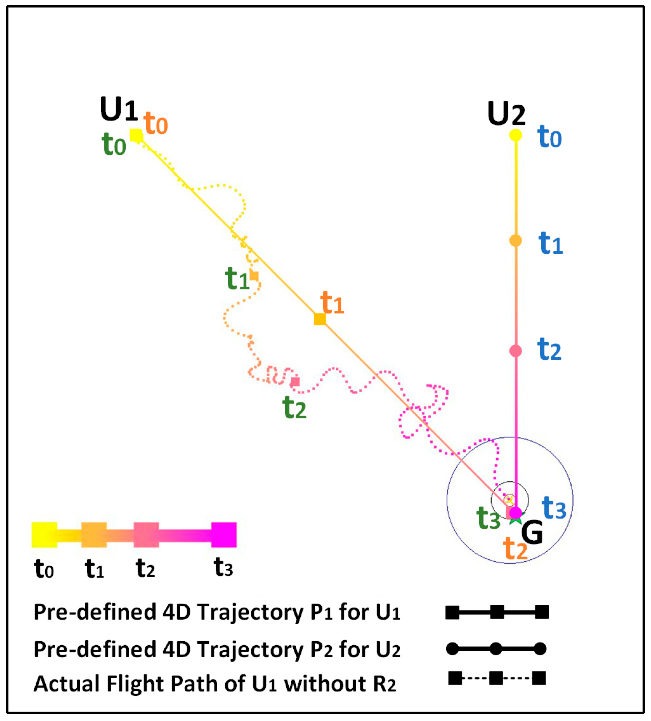
The actual flight trajectories generated by drones  U 1  and  U 2  with and without our ETA-based temporal reward  R 2  are shown in Figure 15 and Figure 16, respectively.
According to the results, it can be seen that, when  U 1  adopted the conflict resolution method without  R 2 , it was unable to reach the next path point  G  at the pre-defined time  t 2  due to executing the tactical conflict resolution strategies. When  U 1  reached the waypoint  G , it was already close to time  t 3 , meaning that there would be a secondary conflict with  U 2  at the waypoint  G . Conversely, in the same scenario with non-cooperative targets, when  U 1  adopted the conflict resolution method with  R 2 , it could still reach  G  at the specified time  t 2  after performing the collision avoidance maneuver with non-cooperative targets, thus avoiding any conflict with  U 2 .
Therefore, the 4D tactical conflict resolution method proposed in this paper based on the ETA can consider the safety avoidance of non-cooperative targets while taking into account the temporal constraints in the strategic 4D trajectory, reducing the occurrence of secondary conflicts caused by the execution of conflict resolution strategies.

6.6. Test 5: Robustness to Uncertainty

6.6.1. Task Setting

The main purpose of this experiment is to verify whether the conflict resolution strategy proposed in this paper can effectively resolve conflicts and ensure flight safety under different levels of noise interference.
In this experiment, the perception of non-cooperative targets in the aforementioned scenario was tested by adding Gaussian noise to the positional information on the non-cooperative targets, with the number of non-cooperative targets set to 15 per square kilometer.

6.6.2. Simulation Results

As shown in Table 4, the method proposed in this paper can still maintain a relatively high success rate of flight missions under three different levels of noise interference, indicating that the proposed method remains effective in the face of positional errors.
In addition, to show the efficiency of our method, the average calculation time of our method was also tested in the above scenarios. The result is listed in Table 4, and it is clearly seen that our method is sufficiently efficient.

6.7. Test 6: Ablation Study

6.7.1. Task Setting

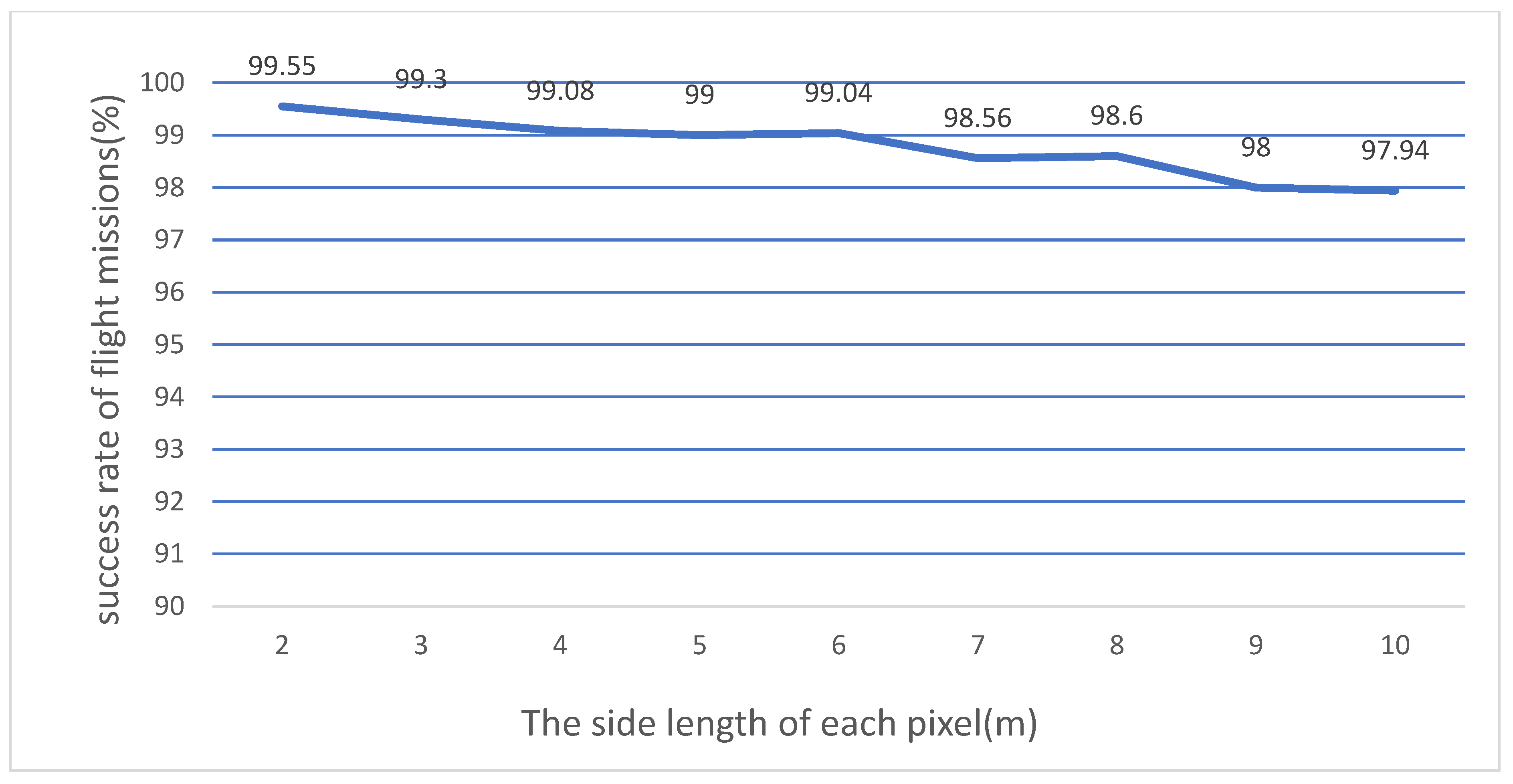
The main purpose of this experiment is to verify whether the method proposed in this paper can maintain good performance in scenarios of different scales.
In this experiment, the perception of non-cooperative targets in the aforementioned scenario was tested by setting the length that each pixel can represent while keeping the number of non-cooperative targets at 15 per square kilometer.

6.7.2. Simulation Results

According to Figure 17, it can be observed that the method proposed in this paper can still maintain a high success rate of flight missions as the length of each pixel represents increases. The slight decrease in the success rate of flight missions is possibly due to the heterogeneous distribution, which can cause a more extreme case with an increased number of non-cooperative targets, leading to the failure of conflict resolution.

7. Conclusions

While the tactical conflict resolution problem is fundamental in air logistics transportation, it is not an exaggeration to say that existing methods have not yet met the standard requirements for success rates in multi-target and high-density collision avoidance scenarios. In this paper, by introducing the risk sector concept and reconstructing the state space, our method achieved a 40.59% improvement in success rate compared with an existing method. Moreover, as existing methods do not consider the temporal constraints at the strategic level, a novel ETA-based temporal reward setting was designed. The combination of these contributions allowed our tactical conflict resolution method to generate a feasible collision-free path to the next waypoint while ensuring a specific arrival time under the temporal constraints of a pre-defined 4D trajectory. In future work, we aim to extend our method to tackle more practical scenarios, such as environments with cooperative targets.

Author Contributions

Conceptualization, C.L.; methodology, Y.Z.; software, W.G.; validation, W.G.; writing—original draft, W.G.; writing—review and editing, L.H., Y.Z. and X.Z. All authors have read and agreed to the published version of the manuscript.

Funding

This work was supported by the Civil Aviation Flight University of China (No. ZJ2021-03), the Civil Aviation Administration of China (No. MHJY2022032) and the Natural Science Foundation of Sichuan Province (No. 2023NSFSC0903).

Data Availability Statement

The data presented in this study are available from the corresponding author upon request.

Conflicts of Interest

The authors declare no conflict of interest.

Abbreviations

SymbolsDefinition
ETAEstimated Time of Arrival
ICAOInternational Civil Aviation Organization
4DT4D Trajectory
4-PNV4D Trajectory Planning, Negotiation, and Verification
MCTSMonte Carlo Tree Search
DQNDeep Q Network
DDPGDeep Deterministic Policy Gradient
USSUAS Service Supplier
  x t 0 the initial state of the drone
  x t f the final state of the drone
  J 1 the hazard cost function
  J 2 the temporal difference cost function
  t f the estimated time of arrival of the drone
at the next waypoint under present situation
  t the specific time of arrival
  R 1 the risk of the drone colliding with the static obstacle  X i 1  
  X i 1 the static obstacle
  R 2 the risk of the drone colliding with the non-cooperative target  X i 2  
  X i 2 the non-cooperative target
  v k the flight speed of the drone at the moment  k  
  a k the acceleration of the drone at the moment  k  
  R 3 mission reward
  ω k the yaw angular velocity
  x k horizontal coordinates
  y k vertical coordinates
  D min k the minimum distance between the drone and the nearest non-cooperation target
  S k the agent’s state space  S  at time  k  
  S k 1 the status information of the drone itself
  S k 2 4D trajectory temporal information
  S k 3 the threatening status information
  R 1 collision avoidance reward
  R u 1 subitem of  R 1  
  r u 1 subitem of  R u 1  
  c 1 constant reward
  r u 2 subitem of  R u 1  
  R u 2 penalize on collision, subitem of  R 1  
  c 2 constant reward
  c 3 collision threshold
  V min the slowest speed
  R 2 an ETA-based temporal reward
  r e the early arrival penalty
  r l the late arrival penalty
  t r   the arrival time difference
  V the weighted velocity that changes as the current state changes
  p k t the normalized remaining time
  p k d the normalized remaining distance
  d t the time window threshold
  D k i s j the distance between the drone and any static obstacles  s j .
  V max the fastest speed
  D n the position of the closest non-cooperative target in  n -th sector
  R g 1 subitem of  R 3  
  R g 2 subitem of  R 3  
  r 3 1 the line-of-sight reward
  r 3 2 the destination distance reward
MDPMarkov Decision Process
  d 1 k the distance between the drone and the next waypoint at time  k  
  α r 3 1 the reward coefficients
  α r 3 2 the reward coefficients
  θ k the yaw angle

References

  1. Global Drone Delivery Market—Analysis and Forecast, 2023 to 2030. Available online: https://www.asdreports.com/market-research-report-575426/global-drone-delivery-market-analysis-forecast (accessed on 8 November 2022).
  2. Dahle, O.H.; Rydberg, J.; Dullweber, M.; Peinecke, N.; Bechina, A.A.A. A proposal for a common metric for drone traffic density. In Proceedings of the 2022 International Conference on Unmanned Aircraft Systems (ICUAS), Dubrovnik, Croatia, 21–24 June 2022; IEEE: Piscataway, NJ, USA, 2022; pp. 64–72. [Google Scholar]
  3. Bradford, S.; Kopardekar, P. FAA/NASA UAS Traffic Management Pilot Program (UPP) UPP Phase 2 Final Report. In FAA/NASA Unmanned Aerial Systems Traffic Management Pilot Program Industry Workshop; NASA: Washington, DC, USA, 2021. [Google Scholar]
  4. Mohamed Salleh, M.F.B.; Low, K.H. Concept of operations (ConOps) for traffic management of Unmanned Aircraft Systems (TM-UAS) in urban environment. In AIAA Information Systems-AIAA Infotech@ Aerospace; American Institute of Aeronautics and Astronautics, Inc.: Reston, VA, USA, 2017; p. 0223. [Google Scholar]
  5. Arafat, M.Y.; Moh, S. JRCS: Joint routing and charging strategy for logistics drones. IEEE Internet Things J. 2022, 9, 21751–21764. [Google Scholar] [CrossRef]
  6. Huang, H.; Savkin, A.V.; Huang, C. Reliable path planning for drone delivery using a stochastic time-dependent public transportation network. IEEE Trans. Intell. Transp. Syst. 2020, 22, 4941–4950. [Google Scholar] [CrossRef]
  7. Khan, A. Risk Assessment, Prediction, and Avoidance of Collision in Autonomous Drones. arXiv 2021, arXiv:2108.12770. [Google Scholar]
  8. Siqi, H.A.O.; Cheng, S.; Zhang, Y. A multi-aircraft conflict detection and resolution method for 4-dimensional trajectory-based operation. Chin. J. Aeronaut. 2018, 31, 1579–1593. [Google Scholar]
  9. Peinecke, N.; Kuenz, A. Deconflicting the urban drone airspace. In Proceedings of the 2017 IEEE/AIAA 36th Digital Avionics Systems Conference (DASC), St. Petersburg, FL, USA, 17–21 September 2017; IEEE: Piscataway, NJ, USA, 2017; pp. 1–6. [Google Scholar]
  10. Chen, T.; Zhang, G.; Hu, X.; Xiao, J. Unmanned aerial vehicle route planning method based on a star algorithm. In Proceedings of the 2018 13th IEEE conference on industrial electronics and applications (ICIEA), Wuhan, China, 31 May–2 June 2018; IEEE: Piscataway, NJ, USA, 2018; pp. 1510–1514. [Google Scholar]
  11. Maini, P.; Sujit, P.B. Path planning for a uav with kinematic constraints in the presence of polygonal obstacles. In Proceedings of the 2016 international conference on unmanned aircraft systems (ICUAS), Arlington, VA, USA, 7–10 June 2016; IEEE: Piscataway, NJ, USA, 2016; pp. 62–67. [Google Scholar]
  12. Abhishek, B.; Ranjit, S.; Shankar, T.; Eappen, G.; Sivasankar, P.; Rajesh, A. Hybrid PSO-HSA and PSO-GA algorithm for 3D path planning in autonomous UAVs. SN Appl. Sci. 2020, 2, 1805. [Google Scholar] [CrossRef]
  13. Khatib, O. Real-time obstacle avoidance for manipulators and mobile robots. Int. J. Robot. Res. 1986, 5, 90–98. [Google Scholar] [CrossRef]
  14. Wang, Z.; Zhou, X.; Xu, C.; Gao, F. Geometrically constrained trajectory optimization for multicopters. IEEE Trans. Robot. 2022, 38, 3259–3278. [Google Scholar] [CrossRef]
  15. Howard, T.M.; Green, C.J.; Kelly, A.; Ferguson, D. State space sampling of feasible motions for high-performance mobile robot navigation in complex environments. J. Field Robot. 2008, 25, 325–345. [Google Scholar] [CrossRef]
  16. Mankiewicz, R.H. Organisation de l’aviation civile internationale. In Global Air Traffic Management Operational Concept; ICAO: Montreal, QC, Canada, 2005. [Google Scholar]
  17. Florence, H.O.; HO, F. Scalable Conflict Detection and Resolution Methods for Safe Unmanned Aircraft Systems Traffic Management. Ph.D. Thesis, The Graduate University for Advanced Studies, Hayama, Japan, 2020. [Google Scholar]
  18. Gardi, A.; Lim, Y.; Kistan, T.; Sabatini, R. Planning and negotiation of optimised 4D trajectories in strategic and tactical re-routing operations. In Proceedings of the 30th Congress of the International Council of the Aeronautical Sciences, ICAS, Daejeon, Republic of Korea, 25–30 September 2016; Volume 2016. [Google Scholar]
  19. Qian, X.; Mao, J.; Chen, C.H.; Chen, S.; Yang, C. Coordinated multi-aircraft 4D trajectories planning considering buffer safety distance and fuel consumption optimization via pure-strategy game. Transp. Res. Part C Emerg. Technol. 2017, 81, 18–35. [Google Scholar] [CrossRef]
  20. Chaimatanan, S.; Delahaye, D.; Mongeau, M. Aircraft 4D trajectories planning under uncertainties. In Proceedings of the 2015 IEEE Symposium Series on Computational Intelligence, Cape Town, South Africa, 7–10 December 2015; IEEE: Piscataway, NJ, USA, 2015; pp. 51–58. [Google Scholar]
  21. FAA, Eurocontrol Pursue Initial Trajectory-Based Operations Now, Full Implementation Later. Available online: https://interactive.aviationtoday.com/avionicsmagazine/july-august-2022/faa-eurocontrol-pursue-initial-trajectory-based-operations-now-full-implementation-later/ (accessed on 15 November 2022).
  22. 4D Skyways Improving Trajectory Management for European Air Transport. Available online: https://www.eurocontrol.int/project/4d-skyways (accessed on 15 November 2022).
  23. Park, J.W.; Oh, H.D.; Tahk, M.J. UAV collision avoidance based on geometric approach. In Proceedings of the 2008 SICE Annual Conference, Chofu, Japan, 20–22 August 2008; IEEE: Piscataway, NJ, USA, 2008; pp. 2122–2126. [Google Scholar]
  24. Strobel, A.; Schwarzbach, M. Cooperative sense and avoid: Implementation in simulation and real world for small unmanned aerial vehicles. In Proceedings of the 2014 International Conference on Unmanned Aircraft Systems (ICUAS), Orlando, FL, USA, 27–30 May 2014; IEEE: Piscataway, NJ, USA, 2014; pp. 1253–1258. [Google Scholar]
  25. Marchidan, A.; Bakolas, E. Collision avoidance for an unmanned aerial vehicle in the presence of static and moving obstacles. J. Guid. Control. Dyn. 2020, 43, 96–110. [Google Scholar] [CrossRef]
  26. Roadmap, A.I. A Human-Centric Approach to AI in Aviation; European Aviation Safety Agency: Cologne, Germany, 2020.
  27. Brat, G. Are we ready for the first easa guidance on the use of ml in aviation. In Proceedings of the SAE G34 Meeting, Online, 18 May 2021. [Google Scholar]
  28. Yang, X.; Wei, P. Autonomous on-demand free flight operations in urban air mobility using Monte Carlo tree search. In Proceedings of the International Conference on Research in Air Transportation (ICRAT), Barcelona, Spain, 26–29 June 2018; Volume 8. [Google Scholar]
  29. Chen, Y.; González-Prelcic, N.; Heath, R.W. Collision-free UAV navigation with a monocular camera using deep reinforcement learning. In Proceedings of the 2020 IEEE 30th International Workshop on Machine Learning for Signal Processing (MLSP), Espoo, Finland, 21–24 September 2020; IEEE: Piscataway, NJ, USA, 2020; pp. 1–6. [Google Scholar]
  30. Cetin, E.; Barrado, C.; Munoz, G.; Macias, M.; Pastor, E. Drone navigation and avoidance of obstacles through deep reinforcement learning. In Proceedings of the 2019 IEEE/AIAA 38th Digital Avionics Systems Conference (DASC), San Diego, CA, USA, 8–12 September 2019; IEEE: Piscataway, NJ, USA, 2019; pp. 1–7. [Google Scholar]
  31. Wan, K.; Gao, X.; Hu, Z.; Wu, G. Robust motion control for UAV in dynamic uncertain environments using deep reinforcement learning. Remote Sens. 2020, 12, 640. [Google Scholar] [CrossRef]
  32. Monk, K.J.; Rorie, C.; Smith, C.; Keeler, J.; Sadler, G.; Brandt, S.L. Unmanned Aircraft Systems (UAS) Integration in the National Airspace System (NAS) Project: ACAS-Xu Run 5 Human-In-The-Loop Sim SC-147 Results Outbrief. In Proceedings of the RTCA Special Committee 147 Face-to-Face Meeting, Phoenix, AZ, USA, 10–13 March 2020. No. ARC-E-DAA-TN73281. [Google Scholar]
  33. ASTM F3548-21; Standard Specification for UAS Traffic Management (UTM) UAS Service Supplier (USS) Interoperability. ASTM: West Conshohocken, PA, USA, 2022; Volume 15.09. [CrossRef]
  34. Fully Automated Instant Delivery Network. Antwork Technology. Available online: https://www.antwork.link (accessed on 5 May 2023).
  35. TCAS Event Recorder. Honeywell. 2021. Available online: https://aerospace.honeywell.com/us/en/about-us/news/2021/09/tcas-event-recorder (accessed on 5 May 2023).
  36. Kopardekar, P.; Rios, J.; Prevot, T.; Johnson, M.; Jung, J.; Robinson, J.E. Unmanned aircraft system traffic management (UTM) concept of operations. In AIAA Aviation and Aeronautics Forum (Aviation 2016); No. ARC-E-DAA-TN32838; NASA: Washington, DC, USA, 2016. [Google Scholar]
  37. Johnson, M. Unmanned Aircraft Systems (UAS) Traffic Management (UTM) Project; NASA: Washington, DC, USA, 2021. Available online: https://nari.arc.nasa.gov/sites/default/files/attachments/UTM%20TIM-Marcus%20Johnson.pdf (accessed on 5 June 2022).
  38. ACSL. Made-in-Japan Drone for Logistics AirTruck. ACSL. 22 December 2022. Available online: https://product.acsl.co.jp/en/wp-content/uploads/2022/12/220627_AirTruck_en_trim.pdf (accessed on 5 May 2023).
  39. Lu, P. Overview of China’s Logistics UAV Industry in 2020. LeadLeo. April 2020. Available online: https://pdf.dfcfw.com/pdf/H3_AP202101071448279174_1.pdf (accessed on 5 May 2023).
  40. 36 Kr Venture Capital Research Institute. Unmanned Distribution Field Research Report. 36 Kr. 26 February 2020. Available online: http://pdf.dfcfw.com/pdf/H3_AP202003041375814837_1.pdf (accessed on 5 May 2023).
  41. Huang, L.Y.; Zhang, D.L. Concept of Operation for UAVs in Urban Ultra-Low-Altitude Airspace. J. Civ. Aviat. 2022, 6, 50–55. [Google Scholar]
  42. Minsky, M. Steps toward artificial intelligence. Proc. IRE 1961, 49, 8–30. [Google Scholar] [CrossRef]
  43. Mnih, V.; Kavukcuoglu, K.; Silver, D.; Rusu, A.A.; Veness, J.; Bellemare, M.G.; Graves, A.; Riedmiller, M.; Fidjeland, A.K.; Ostrovski, G.; et al. Human-level control through deep reinforcement learning. Nature 2015, 518, 529–533. [Google Scholar] [CrossRef] [PubMed]
  44. Van Hasselt, H.; Guez, A.; Silver, D. Deep reinforcement learning with double q-learning. In Proceedings of the AAAI Conference on Artificial Intelligence, Phoenix, AZ, USA, 12–17 February 2016; Volume 30. [Google Scholar]
  45. Wang, Z.; Schaul, T.; Hessel, M.; Hasselt, H.; Lanctot, M.; Freitas, N. Dueling network architectures for deep reinforcement learning. In Proceedings of the International Conference on Machine Learning, PMLR, New York, NY, USA, 20–22 June 2016; pp. 1995–2003. [Google Scholar]
  46. ICAO Model UAS Regulations. Available online: https://www.icao.int/safety/UA/Pages/ICAO-Model-UAS-Regulations.aspx (accessed on 18 November 2022).
  47. Mo, S.; Pei, X.; Chen, Z. Decision-making for oncoming traffic overtaking scenario using double DQN. In Proceedings of the 2019 3rd Conference on Vehicle Control and Intelligence (CVCI), Hefei, China, 21–22 September 2019; IEEE: Piscataway, NJ, USA, 2019; pp. 1–4. [Google Scholar]
  48. Fang, S.; Chen, F.; Liu, H. Dueling Double Deep Q-Network for Adaptive Traffic Signal Control with Low Exhaust Emissions in A Single Intersection. IOP Conf. Ser. Mater. Sci. Eng. 2019, 612, 052039. [Google Scholar] [CrossRef]
  49. Han, B.A.; Yang, J.J. Research on adaptive job shop scheduling problems based on dueling double DQN. IEEE Access 2020, 8, 186474–186495. [Google Scholar] [CrossRef]
  50. Sui, Z.; Pu, Z.; Yi, J.; Xiong, T. Formation control with collision avoidance through deep reinforcement learning. In Proceedings of the 2019 International Joint Conference on Neural Networks (IJCNN), Budapest, Hungary, 14–19 July 2019; IEEE: Piscataway, NJ, USA, 2019; pp. 1–8. [Google Scholar]
  51. Radio Technical Commission for Aeronautics (US). Minimum Operational Performance Standards for Traffic Alert and Collision Avoidance System (TCAS) Airborne Equipment; Radio Technical Commission for Aeronautics: Washington, DC, USA, 1983. [Google Scholar]
  52. Indian Defence Review. Aviation: The Future Is Unmanned. Available online: http://www.indiandefencereview.com/news/aviation-the-future-is-unmanned/2/ (accessed on 18 January 2023).

Figure 1. Schematic diagram of urban logistics drone operation [34].
Drones 07 00334 g001
Figure 2. TCAS II typical envelope [35].
Drones 07 00334 g002
Figure 3. Block diagram of reinforcement learning.
Drones 07 00334 g003
Figure 4. A detailed framework of Dueling Double DQN for the UAV tactical conflict resolution problem.
Drones 07 00334 g004
Figure 5. Schematic diagram of the risk sector.
Drones 07 00334 g005
Figure 6. Schematic diagram of  d 1 d 2 , and  ψ k .
Drones 07 00334 g006
Figure 7. Simulation scenario.
Drones 07 00334 g007
Figure 8. Pre-planned 4D trajectory.
Drones 07 00334 g008
Figure 9. Loss error values.
Drones 07 00334 g009
Figure 10. Reward values.
Drones 07 00334 g010
Figure 11. Success rates of flight missions with and without “risk sector”.
Drones 07 00334 g011
Figure 12. Punctuality results for different strategies.
Drones 07 00334 g012
Figure 13. Average number of accidents per 10,000 flight hours over different densities.
Drones 07 00334 g013
Figure 14. Pre-planned 4D trajectories for two cooperative target drones.
Drones 07 00334 g014
Figure 15. The flight trajectory generated by the strategy without  R 2 .
Drones 07 00334 g015
Figure 16. The flight trajectory generated by the strategy with  R 2 .
Drones 07 00334 g016
Figure 17. The success rates of different side lengths of pixels.
Drones 07 00334 g017
Table 1. Action Space.
a k ( m / s 2 ) −303
ω k ( r a d / s )
π 30   ( π 30 , 3 )   ( π 30 , 0 )   ( π 30 , 3 )
0   ( 0 , 3 )   ( 0 , 0 )   ( 0 , 3 )
  π 30   ( π 30 , 3 )   ( π 30 , 0 )   ( π 30 , 3 )
Table 2. Settings of hyper-parameters.
ParameterValue
Learning rate0.00005
Discount factor0.99
buffer_size1,000,000
batch_size256
Multi-step update5
Update delay of current network10 steps
Update delay of target networkUpon completion of each round
Total number of training rounds5000
Loss functionMSE
Table 3. Detailed testing results under different strategies.
without   r e     and   r l with   r l with   r e with   r e   and   r l
Success rate of flight missions (%)99.5899.1699.6499.11
Early to waypoint (s)5355.44213.2414.343
Late to waypoint (s)55.67321.15365.60523.417
On-time rate (%)
with time window {−10 s, 10 s}
3.151.206.3816.34
On-time rate (%)
with time window {−15 s, 15 s}
4.451.5010.2024.82
On-time rate (%)
with time window {−20 s, 20 s}
5.351.8614.5438.16
On-time rate (%)
with time window {−25 s, 25 s}
6.292.1519.5064.56
On-time rate (%)
with time window {−30s, 30 s}
7.352.3325.0984.55
Table 4. Success rates of flight missions and calculation times under different noise scenarios.
Average Magnitude of ErrorVarianceSuccess Rate of Flight Missions (%)Average Calculation Time (s)
10.2599.5%0.001003
50.2599.34%0.001074
100.2598.92%0.000998
Disclaimer/Publisher’s Note: The statements, opinions and data contained in all publications are solely those of the individual author(s) and contributor(s) and not of MDPI and/or the editor(s). MDPI and/or the editor(s) disclaim responsibility for any injury to people or property resulting from any ideas, methods, instructions or products referred to in the content.