Scheduling Drones for Ship Emission Detection from Multiple Stations

Abstract

Various port cities and authorities have established emission control areas (ECAs) to constrain ships’ fuel usage in a specified offshore geographical range. However, these ECA policies involve high costs and have low monitoring and regulation enforcement efficiencies. In this study, a meeting model was used to investigate the drone-scheduling problem by considering the simultaneous movements of drones and ships. Set-covering integer linear programs were developed to formulate the assignments of drones to ships, and a model and solution algorithm were devised to determine the moving times and meeting positions for particular drones and ships. The proposed models and algorithms were employed and verified in experiments. The flying times for the datasets with three drone base stations were shorter than those with two. More drones resulted in shorter flying distances. The use of the meeting model enabled the acquirement of shorter flying times and distances than when it was not used. The datasets with more ships had longer flying times and distances, with almost linear relationships. The sensitivity of the effect of varying 5% of the ships’ speeds on the flying time metrics was less than 1%, affecting the flying distance by about 4–5%. Accelerating the drones was more effective towards optimizing the drones’ flying distances than times. Numerical studies showed that the consideration of simultaneous movements in the model allowed for a reduction in the drones’ flying distances and increased efficiency. Based on the modeling and experimental studies, managerial implications and possible extensions are discussed.

1. Introduction

Shipping is the primary transport mode for the trade of commodities and emits many air pollutants. The atmospheric pollutants discharged by ships seriously impact the natural environment and public health, and their fundamental source is heavy oil [1]. The pollutants emitted from the combustion of ship fuel generally include sulfur oxides, nitrogen oxides, carbon oxides, and particulate matter, among which sulfur oxides and nitrogen oxides are the most harmful to the atmosphere and human beings [2]. As few tail gas filters are installed in ships, the tail gas pollutants drift to coastal and inland port cities with the wind, thereby aggravating urban environmental pollution. Sulfide and nitride produced by heavy oil consumption seriously impact the natural environment and public health. The problem of ship exhaust emissions is a global environmental protection problem. The tail gas generated by the burning of heavy oil on various ships contains sulfide, nitrogen oxides, and other toxic and harmful substances, causing long-term harm to port cities and coastal residents and, further, resulting in global environmental protection problems. Given the unique position of shipping in world trade, reducing sulfur emissions from ships is of great significance for improving air quality in port areas and port cities and protecting the environment in coastal regions and the ecology of the whole planet. To reduce emissions of atmospheric pollutants from ships, governments and organizations have established emission control areas (ECAs) in which the use of heavy oil in/on ships is controlled [3]. The relevant international organizations and national governments have set strict requirements regarding the sulfur content of the fuel used for ships in these emission control zones. However, light oil is more expensive than heavy oil. Thus, ship owners may use heavy oil and violate these regulations to reduce costs.

To address the problem of ship emissions polluting the atmosphere around port cities, the most common solution is to establish ship emission control zones around ports. In these areas, ships are required to use high-quality fuel to reduce relevant pollutant emissions. Although laws and regulations related to exhaust emission control areas have been issued, as high-quality fuel increases the navigation costs of ships, violations are common. For the supervision of ship exhaust emissions, current practices require many supervisors to screen or conduct surprise inspections of incoming and outgoing ships, which is insufficient in terms of monitoring strength and coverage and wastes many workers and material resources [4]. Drone-sniffing technology is used for the periodic monitoring of ECAs, which has the advantages of being fast, highly secure, and highly efficient; effecting no regional impact; and having good inspection quality [5]. Applying this monitoring method, along with the optimization and improvement of patrol inspection paths through scientific methods, can significantly increase the intensity and coverage of sulfur emission monitoring in emission control areas, help thoroughly crack down on illegal emissions, effectively curb illegal emissions, and effectively promote the implementation of numerous environmental regulations, including the ECA and sulfur limitation regulations, which would be of great significance for the regulation of ship exhaust emissions and the improvement of the global environment. There are many alternative methods for ship emission detection, e.g., the use of specialized patrol ships and airplanes. However, these methods are expensive and generate additional pollution themselves. Maritime drones have the significant advantages of a fast response speed, comprehensive coverage, low operating costs, and low safety risks when carrying mission loads such as optoelectronic equipment, airborne automatic identification systems (AISs), airborne VHF, hyperspectral imaging equipment, sea search radars, and oil pollution sampling equipment to undertake the main functions related to cruise law enforcement, administrative inspection, search and rescue during emergencies, responses to oil (chemical) pollution emergencies, communication relays, maritime security, and navigation mapping. At the same time, due to the wide range of sea patrol areas and the uncertainty of climate conditions, the use of drones also incurs related costs. Therefore, patrol paths should be optimized to reduce the operational costs of drones.

This study examined the drone-scheduling problem with multiple drone base stations. In an ECA, multiple drone base stations cooperate in managing emission detection tasks via the scheduling of drones. Typically, a drone base station determines which drone to dispatch to inspect ships’ exhaust gas and when. At the station, AIS receivers are used to detect offshore ships and verify whether they have crossed the ECA borders or are floating in the ECA. Then, the station dispatches drones to engage the ships based on the ships’ positions, velocities, and movement directions. The AIS receivers obtain these data or estimate them based on the received data. However, ships may travel over a long range in an ECA, especially in long belts. Therefore, it is necessary to coordinate the drone base stations to handle the ships and detect their emissions once in the ECA, and if the ships do not leave the ECA, it can be presumed that they will not change fuel. In other words, the drone base stations should cooperatively determine the detection frequency to reduce the operation costs while ensuring the administrative effects.

This study contributes to the studies on ECA administration and drone-scheduling problems. In studies on ECAs, the policies and operation methods are examined. Following on from previous research and practices in ship emission detection, this study investigates the possibility of and operation models for using drones as a new and emerging technology in ECA studies. Indeed, using drones in ship emission detection has been tested and examined in practice. However, it has two distinct features that must be addressed. First, the ships are moving when the drones are scheduled and flying towards the ships. Therefore, the drone and the ship to be detected should be coordinated. A model is formulated to compute the position and time for a flying drone to meet the ship to be detected, which is called a meeting model. Second, the drone base stations should decide which station undertakes the detection task and schedule a drone. The problem of assigning drones to ships is formulated as an integer program considering immobile ships, and the integer program further incorporates the meeting model to support mobile ships.

In Figure 1, a systematic flow diagram describes the research problem, features, models, and solution methods. The formulation and solution methods’ development is organized in Section 3, Section 4 and Section 5 by considering the drone stations and ECA sides. In Section 3, the ships are presumed to be immobile, and the drones fly from the drone stations to conduct emission detection. An integer problem, [M1], is developed as a baseline model to assign drones to ships. Then, considering the movements of ships while the drones are flying to detect their emissions, a meeting model, [M2], is developed. An algorithm (DA) is then devised to solve it. In Section 5, the meeting model is incorporated into a new model, [M3], to consider the simultaneous movements of drones and ships. We conduct a series of numerical experiments to examine the proposed models and algorithms in Section 6. Finally, we conclude the study in Section 7.

2. Related Studies

2.1. Emission Control Area (ECA)

The pollution from shipping exhaust has become the third largest source of air pollution after vehicle exhaust and that produced by industrial enterprises. Most ports are concentrated in densely populated areas along coasts and rivers, and carcinogenic waste gases envelop port cities, causing great harm to their residents. There is an urgent need to strengthen the control of shipping pollution. SOx, NOx, and PM2.5 emitted by ships are some of the “main culprits” of air pollution in port cities, which seriously endanger human health [6].

An ECA is established to control the emission of atmospheric pollutants from ships. It reduces the emission of sulfide and nitride by limiting the use of heavy oil. When ships are near the sea, they often travel along the coastline, and thus the ECA is ribbon-shaped. When a ship sails in an inland sea, its navigation area often presents the outline of the inland sea. In both cases, the moving space of the ship is continuous. Current control areas are usually established in sea areas close to land to reduce the impact of atmospheric emissions from ships on the natural environment and human health.

Therefore, it is necessary to take adequate measures to monitor the discharge of ships in an emission control area, which can be used as an auxiliary basis to judge whether ships use heavy oil.

Table 1. Pioneering studies on emission control areas.

Study	Research Problem	Method	Region/Port
[7]	An ECA location problem minimizes the impact of sulfur emissions on human health.	MILP	China + Africa
[8]	Impacts of ECA regulations on port efficiency.	DEA	EU + North America
[9]	Reduction in fuel costs by rescheduling voyage plans, speeds, and sailing patterns.	MILP + Tabu	-
[10]	The impacts of ECAs on global shipping; route-choosing behavior of liner shipping through ECAs.	A	Mediterranean Sea
[11]	Impacts of Panama Canal Authority pollution tax on emissions from ships transiting the Panama Canal.	A	Panama Canal
[12]	Rescheduling of ports-of-call sequences, ship routes, and speed to minimize total sailing costs.	NLP + GA	North America
[13]	Coordination of ECA programs to align conflict interests between governments and shipping companies.	EGT	China
[14]	The trade-off between cost and emission (CO2 and SOx) reduction considering ECAs.	MILP + GA	-
[15]	Green vessel schedule recovery strategies, including vessel sailing speed adjustment and port skipping.	NLP	-
[16]	Assessment of the effect of China’s ECA policy and determination of the optimal ECA width.	BLP	China
[17]	Examination of dual environmental effects of ECAs on liner service markets.	A	Shanghai + Persian Gulf
[18]	The undertaking of route and speed optimization to simultaneously reduce sailing cost and time, considering ECA regulations and weather conditions.	MOP + TOPSIS	US Coast
[19]	ECA boundary design and emission reduction assessment.	NLP	North America
[20]	Optimization of vessel speeds and ship fleet sizes considering ECAs.	NLP
[21]	Investigation of potentially varying effectiveness of ECA policies in port cities located in a specific region.	A	China
[22]	A total emission control method with an emphasis on environmentally sensitive water areas.	A	Yangtze Delta
[23]	Impacts of emission tax on vessel and port operations for emission control in port areas.	GT	-
[24]	Impacts of ECAs on reduction in SO2 concentrations.	A	China

Note: A = analytical data-driven or principal models; BLP = bi-level program; DEA = data envelopment analysis; EGT = evolutionary game model; EU = European Union; GA = genetic algorithm; GT = game theory; MILP = mixed-integer linear program; MOP = multi-objective optimization; NLP = non-linear program; Tabu = tabu search.

summarizes studies on ECAs according to three aspects: the problem features, methods, and corresponding regions or ports. ECAs are a general emission control solution, so most governments and ports have developed policy tools. The investigated studies focus on various problem features, including ECA shaping, impact assessment, ECA-based scheduling optimization, and stakeholders’ behaviors. The studies use four methods: data-driven or principal analytical methods, and methods involving optimization, behavior, and assessment. In summary, the ECA studies range widely and correlate with many aspects and levels.

2.2. Drone-Scheduling Problem

Among the existing ship emission monitoring methods, the use of drones is a good choice because the operating mode of drones offers the advantages of automation; the unmanned, accurate collection of information; and the timely transmission of information, and it can overcome geographical obstacles [5]. However, the fixed cost of purchasing drones and the variable cost of using drones are still high. Optimizing the flight path of drones can reduce the cost of their use. At present, many countries have begun to use the monitoring method of using fixed-wing aircraft and gas sensors to achieve emission control area supervision, that is, using fixed-wing aircraft carrying a variety of high-precision gas detection sensors or gas collection devices to monitor ship exhaust in emission control areas [25]. Compared with the previous cumbersome processes, such as law enforcement personnel boarding, document inspection, fuel sampling, and detection, drone-based monitoring has dramatically improved the efficiency of supervision and can achieve non-contact supervision.

A ship emission monitoring system comprises an exhaust-gas-sensing module, a power supply system, a pod shell, an exhaust gas data control system, a processing and transmission system, a GPS (Global Positioning System) module, a drone-control-end software system, and a server-end software system. Users can attach the ship emission monitoring system to the drone rack and control part of the working state of the monitoring pod system through GSM (Global System for Mobile Communications) mode at the remote-control-end of the drones during the actual operation of the system. At the same time, the ship-emission-monitoring system transmits the obtained exhaust monitoring data and GPS data to the data server through GPRS (General Packet Radio Services).

The drone flight platform is classified into multi-rotor drones, fixed-wing drones, unmanned helicopters, and composite-wing drones in terms of morphology. Considering that the drones need to achieve accurate hovering and synchronous movement at the position at which exhaust is being emitted from the ship when monitoring its emission of pollutive gas, each drone needs to have strong maneuverability, excellent portability, extensive expansion, and other characteristics. A multi-rotor drone is suggested as a flight platform for patrolling, law enforcement, and evidence collection.

In

Table 2. Pioneering studies on drone-scheduling problems.

Study	Research Problem	Methods	Scenario
[26]	The flying speed of the drone is optimized while ensuring that it completes the route within a specific time and without depleting its battery.	NLP + DP	Surveillance
[27]	Energy trading between the drones and charging station.	GT	Delivery
[28]	A parcel delivery system using drones.	MILP + H	Delivery
[29]	Parallel drone-scheduling-oriented traveling salesman problem; a set of customers requiring a delivery is split between a truck and a fleet of drones.	MILP + H	Delivery
[30]	Drone mobility in the lateral or vertical path leads to a time-selective and frequency-selective wireless channel for a low-altitude drone.	A	Communication
[31]	A drone-based delivery-scheduling method considering drone failures to minimize the expected loss of demand.	SA	Delivery
[32]	Drone flight scheduling under uncertainty of battery duration and air temperature.	ML	-
[33]	A hybrid battery-charging approach with dynamic wireless charging systems.	NLP	-
[34]	A drone-based diagnostic testing kit delivery-scheduling problem with one truck and multiple drones.	H	Emergency delivery
[35]	Authentication of drones and verification of their charging transactions with charging stations.	PSO + GT	-
[36]	Delivery of perishable items to remote areas accessible only by helicopters or drones.	A	Emergency delivery
[37]	A drone-scheduling problem regarding the delivery of small parcels to remote islands considering wind direction and speed.	RO	Island delivery
[38]	Coordinating a truck and multiple heterogeneous drones for last-mile package deliveries.	SA + VNS VNS	Delivery
[39]	5G-powered drone video transmission.	ML	Video streaming
[40]	On-time delivery of packages.	MILP GA + PSO	Warehouse
[41]	Deriving actions at a battery swap station when explicitly considering the uncertain arrival of swap demand, battery degradation, and replacement.	DP	Delivery

Note: DP = dynamic programming; H = heuristics; MILP = mixed-integer linear program; ML = machine learning; NLP = non-linear program; PSO = particle swarm optimization; RO = robust optimization; SA = simulated annealing; VNS = variable neighborhood search.

, we summarize some pioneering studies according to three aspects. The drone-scheduling problem occurs in various scenarios, mainly delivery, surveillance, and communication relay systems. Related to this study, the applications for delivery (mainly including emergency delivery and city logistics) can inspire the development of models and algorithms. We can observe three distinct features of the drone-scheduling problem, including the coordination between drones and other devices (e.g., trucks), the battery and its endurance problem, and the dynamics of the drone flight and services. In the context of ship emission detection, the drone-scheduling problem also reflects these features to some extent.

3. Scheduling Drones for Immobile Ships

In the following section, we investigate the drone-scheduling problem in three steps. First, the ships wait at the positions, and the drones fly to check the ships’ emissions. Indeed, as our premise, we contend that the drone flying speed should be far greater than the ships’ speed. Second, considering the simultaneous movements of drones and ships, we develop a model to determine the meeting position and time between drones and ships (Section 4). Third, considering the application scenarios with multiple drone stations and ships, we formulate the model for assigning drones to ships considering the meeting model (Section 5).

3.1. Problem Statement

As depicted in Figure 2, two drone base stations dispatch drones for ship emission detection tasks. A drone flies from its host station to the ship (see drone’s flying paths), whose position can be determined by the AIS receiver at the drone’s base station or other facilities connected with the station. However, the presumption that the ship waits for emission detection is not always fulfilled. When the drone flies to the pre-determined position, the ship moves forward in its direction (see ship’s present position, target position, and moving direction in the figure). Notably, when a drone flies to the “present position” of a ship, the ship may move forward to a new position, so the drone must chase the ship (see the drone’s chasing path in the figure).

3.2. Formulation

The drone-scheduling problem described above concerns two sets: the set of ships, I = {1,2,⋯}, indexed by i, and the set of drone base stations, K = {1,2,⋯}, indexed by k. C_ki denotes the time that a drone flies from the station k to the ship i, and Q_k denotes the number of available drones at station k. The binary decision variable $x_{ki}\in \left\{0,1\right\}$ is 1 if the drone base station k dispatches a drone to visit the ship i, and is 0 otherwise. Using these data and variables, the drone-scheduling model [M1] determines the assignment of ships to the drone base stations:

$$\left[\mathrm{M}1\right]\min t={\displaystyle \sum }_{ki}{C}_{ki}{x}_{ki}$$

It is subject to

$${\displaystyle \sum }_k{x}_{ki}=1,\forall i$$

(1)

$${\displaystyle \sum }_i{x}_{ki}\le Q_k,\forall k$$

(2)

$$x_{ki}\in \left\{0,1\right\},\forall k,i$$

(3)

The objective of [M1] is to minimize drones’ flying times. It also equates to the time the ships spend waiting. In Constraint (1), every ship is visited by a drone. In (2), a drone base station can send drones of a limited number to the ships. In the model, it is presumed that there are enough drones for the ships, i.e., $\sum _k{Q}_k\ge \left|I\right|$. In (3), the scheduling relation is formatted using binary variables.

When the drones reach the pre-determined positions, the ships move far from these positions. The total distance $l^{\left[\mathrm{M}1\right]}$ can be calculated by (4). If a drone $i$ tries to chase the ship $k$, the time can be determined by (5). It is presumed that the drones always fly faster than the ships’ movement speeds, i.e., ${\overline{V}}_k-V_i>0$. Moreover, we can compute the time and distance the drone from the base station k spends chasing the ship $i$, which are denoted by $t^{chase}$ and $l^{chase}$ in (5)–(8). In Equation (4), the flying distance is computed using the objective values of [M1]. When the drone from k reaches the original position of the ship i, the ship has moved $C_{ki}{V}_i$ along its direction; thus, considering the simultaneous movements of the drone and ship, the chasing time is computed using (5) with a speed of $\left({\overline{V}}_k-V_i\right)$ for the distance of $C_{ki}{V}_i$. In (6), the total chasing time is the sum of all the drones’ chasing times. Similarly, the chasing distances are determined by (7) and (8).

$$l^{\left[\mathrm{M}1\right]}={\displaystyle \sum }_{ki}{x}_{ki}{C}_{ki}{V}_i$$

(4)

$$t_{ki}^{chase}=\frac{x_{ki}{C}_{ki}{V}_i}{{\overline{V}}_k-V_i}$$

(5)

$$t^{chase}={\displaystyle \sum }_{ki}{t}_{ki}^{chase}$$

(6)

$$l_{ki}^{chase}=\frac{x_{ki}{C}_{ki}{V}_i}{{\overline{V}}_k-V_i}\cdot {\overline{V}}_k$$

(7)

$$l^{chase}={\displaystyle \sum }_{ki}{l}_{ki}^{chase}$$

(8)

The solution to [M1] and its subsequent results are denoted by

$$t^{\left[\mathrm{M}1\right]},l^{\left[\mathrm{M}1\right]},t^{chase},l^{chase}\leftarrow f^{\left[\mathrm{M}1\right]}\left(\left[C_{ki},Q_k|\forall k,i\right]\right).$$

4. A Meeting Model for a Drone and Directional Mobile Ship

4.1. Formulation

As studied above, when the drone flies to the pre-determined position of the ship, the ship will move to its destination position. Therefore, it is beneficial to coordinate the drone and ship movements. We compute the meeting position considering their movements and then dispatch the drone to the estimated position.

A ship i located at $\left(X_i,Y_i\right)$ proceeds in the direction $\left(X_i^t,Y_i^t\right)$, with a moving speed of $V_i$. The drone base station $k$ is located at $\left({\overline{X}}_k,{\overline{Y}}_k\right)$. If the station $k$ dispatches a drone with a speed of ${\overline{V}}_k$ to visit the ship $i$, the drone should fly for time $t$ to meet the ship while the ship is moving in the target direction.

The position at which the drone meets the ship is shown in Figure 3. The ship travels from point $a\left(X_i,Y_i\right)$ to point $b\left(X_i^t,Y_i^t\right)$. We can draw two circles: one for the drone with the center $\left({\overline{X}}_k,{\overline{Y}}_k\right)$ and radius ${\overline{V}}_{k}t$, and the other for the ship with the center $\left(X_i,Y_i\right)$ and radius $V_{i}t$. The intersection of the two circles on line $ab$ is the meeting point. We can compute the intersection by solving model (9), where $V_i^X,V_i^Y$ are given in (10) and (11).

$$\left[\mathrm{M}2\right]\{\begin{array}{c}{x}_i=X_i+t\cdot V_i^X\\ y_i=Y_i+t\cdot V_i^Y\\ \sqrt{{\left(x_i-{\overline{X}}_k\right)}^2+{\left(y_i-{\overline{Y}}_k\right)}^2}=t\cdot {\overline{V}}_k\end{array}$$

(9)

$$V_i^X=V_i\frac{X_i^t-X_i}{\sqrt{{\left(X_i-X_i^t\right)}^2+{\left(Y_i-Y_i^t\right)}^2}}$$

(10)

$$V_i^Y=V_i\frac{Y_i^t-Y_i}{\sqrt{{\left(X_i-X_i^t\right)}^2+{\left(Y_i-Y_i^t\right)}^2}}$$

(11)

4.2. Solution Algorithm

To solve (8), we devised a binary search algorithm with the following steps: First, select the midpoint $\left(x_i,y_i\right)$ of segment $ab$, and compare the time ($t$) when the ship and the drone arrive at this point $\left({\overline{t}}_i,t_i\right)$. If $t_i>{\overline{t}}_i$, then select the midpoint $d$ between $\left(X_i^t,Y_i^t\right)$ and $\left(x_i,y_i\right)$; if $t_i>{\overline{t}}_i$, then select the midpoint between $\left(X_i,Y_i\right)$ and $\left(x_i,y_i\right)$. The specific algorithm is shown in Algorithm 1.

Algorithm 1	Dichotomy algorithm (DA)
Input	$\left(X_i,Y_i\right):$ ship $i$’s position;
	$\left(X_i^t,Y_i^t\right):$ ship $i$’s target position; $\left({\overline{X}}_k,{\overline{Y}}_k\right):$ the drone base position; $V_i$: ship $i$’s speed; ${\overline{V}}_k$: The speed of the drone.
Output	$\left(x_i,y_i,t_i\right)$: the position and time.
Variable	$\left(x_l,y_l\right),\left(x_u,y_u\right)$: the lower and upper bounds of the intersection position of the drone and ship;
	${\overline{t}}_i$: the moment at which the ship begins to travel to the intersection point; $\delta$: tolerance.
Steps
Step 1	Initialize $\left(x_l,y_l\right),\left(x_u,y_u\right)$ and $\left(x_i,y_i\right)$.
	$\left(x_u,y_u\right)\leftarrow \left(X_i,Y_i\right)$; $\left(x_l,y_l\right)\leftarrow \left(X_i^t,Y_i^t\right)$; $\left(x_i,y_i\right)\leftarrow \left(\frac{x_u+x_l}{2},\frac{y_u+y_l}{2}\right)$.
Step 2	Compute $t_i,{\overline{t}}_i$
	$\{\begin{array}{c}{t}_i\leftarrow \frac{\sqrt{{\left({\overline{X}}_k-x_i\right)}^2+{\left({\overline{Y}}_k-y_i\right)}^2}}{{\overline{V}}_k}\\ {\overline{t}}_i\leftarrow \frac{\sqrt{{\left(X_i-x_i\right)}^2+{\left(Y_i-y_i\right)}^2}}{V_i}\end{array}$.
Step 3	While $\left|t_i-{\overline{t}}_i\right|\le \delta$:
Step 3.1	If $t_i>{\overline{t}}_i$:
	$\left(x_u,y_u\right)\leftarrow \left(x_i,y_i\right)$
Step 3.2	Else:
	$\left(x_l,y_l\right)\leftarrow \left(x_i,y_i\right)$
	End if
Step 3.3	Update $\left(x_i,y_i\right)$.
	$\left(x_i,y_i\right)\leftarrow \left(\frac{x_u+x_l}{2},\frac{y_u+y_l}{2}\right)$.
Step 3.4	Update $\left(t_i,{\overline{t}}_i\right)$
	$\{\begin{array}{c}{t}_i\leftarrow \frac{\sqrt{{\left({\overline{X}}_k-x_i\right)}^2+{\left({\overline{Y}}_k-y_i\right)}^2}}{{\overline{V}}_k}\\ {\overline{t}}_i\leftarrow \frac{\sqrt{{\left(X_i-x_i\right)}^2+{\left(Y_i-y_i\right)}^2}}{V_i}\end{array}$.
Step 4	Return $\left(x_i,y_i,t_i\right)$

We can obtain the meeting position $\left(x,y\right)$ and flying time $t^{meet}$ for a drone at the base station $k$ and a ship $i$ using the above model [M2], which is denoted by

$$t^{meet},x_i,y_i\leftarrow f^{\left[\mathrm{M}2\right]}\left({\overline{X}}_k,{\overline{Y}}_k,X_i,Y_i,X_i^t,Y_i^t,{\overline{V}}_k,V_i\right).$$

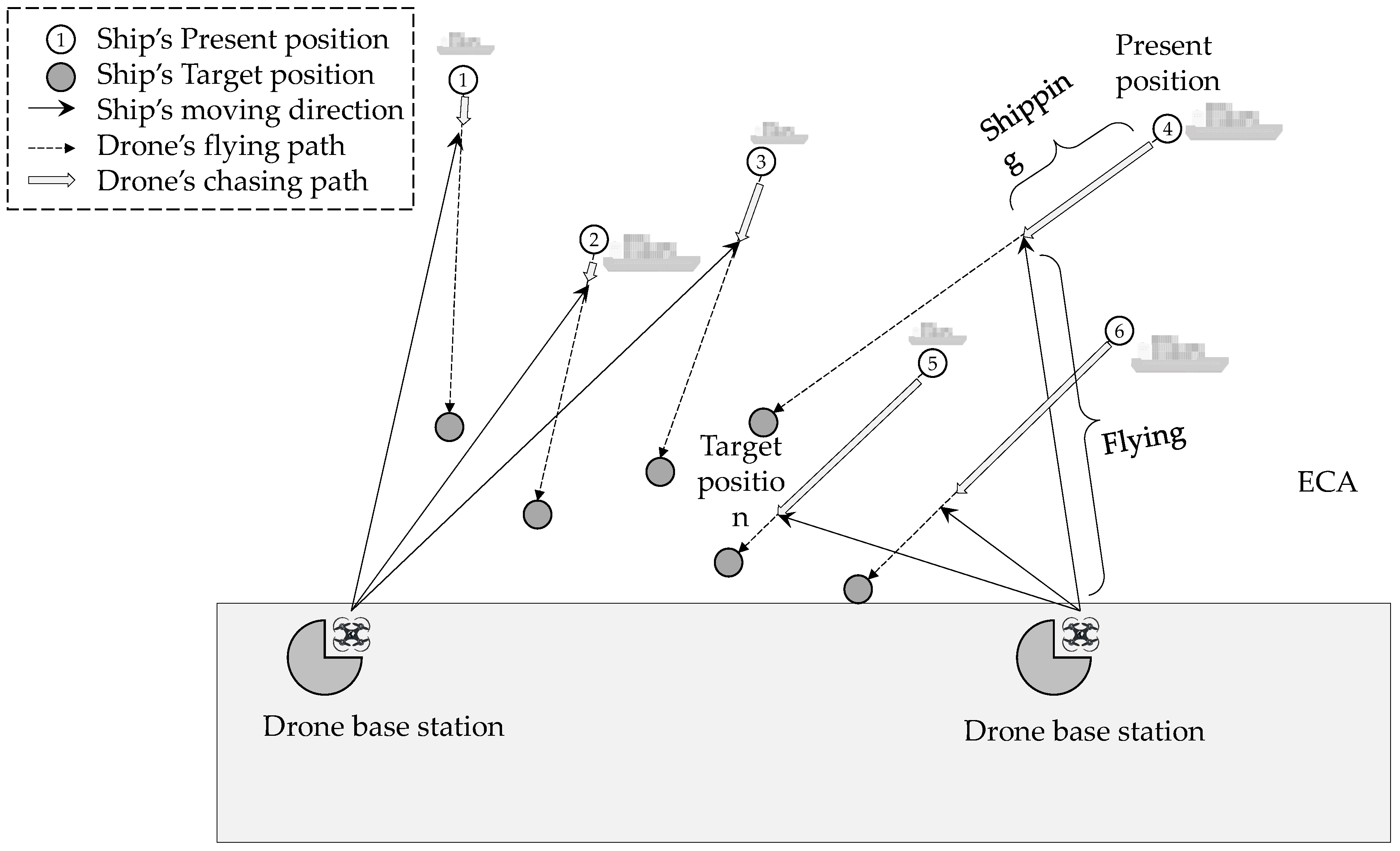
5. Scheduling Drones for Mobile Ships

5.1. Problem Statement

Figure 4 depicts a conceptual diagram of the drone-routing problem based on the ships’ present positions and moving directions. The drones from the left base station fly to ships 1, 2, and 3, while those from the right base station fly to ships 4, 5, and 6. Taking Ship 4′s emission detection as an example in the figure, the ship moves from the present position to the target. The drone from the right base station flies directly to the meeting position.

As shown above, the meeting position can be pre-calculated by $f^{\left[\mathrm{M}2\right]}(\cdot )$.

As demonstrated above, the $k$-th drone base position is $\left({\overline{X}}_k,{\overline{Y}}_k\right)$, the ship set is $I=\left\{1,2,\cdots \right\}$, ship $i$’s position is $\left(X_i,Y_i\right)$, the target position is $\left(X_i^t,Y_i^t\right)$, and the speed is $V_i$. The speed of the drone is ${\overline{V}}_k$. To formulate the drone-routing problem, we introduce a tri-tuple variable $\left(x_i,y_i,t_i\right)$, representing the position and time where the act of detection occurs. Thus, we can order the tuples by $t_i$ to obtain the sequence of visits to the ships, which is denoted by $J$. Additionally, $J^{+}=\left[\left(i,j\right):i,j\in J\cup \left\{0\right\}\right]$ denotes the arc lists starting from the drone base and ending at the base station.

5.2. Formulation

The drone-routing problem is formulated in [M1] using the above notation:

$$\left[\mathrm{M}3\right]\min t={\displaystyle \sum }_{ki}{C}_{ki}{x}_{ki}$$

which is subject to

$$\mathrm{Constraints}\left(\left(1\right),\left(2\right)\right).$$

$$C_{ki}\leftarrow f^{\left[\mathrm{M}2\right]}\left({\overline{X}}_k,{\overline{Y}}_k,X_i,Y_i,X_i^t,Y_i^t,{\overline{V}}_k,V_i\right),\forall k,i$$

(12)

Formally, [M3] does not change the form of [M1] but changes the parameter ($C_{ki}$)’s generation scheme. [M1] and [M3] are both typical set-covering integer linear program problems solvable by on-the-shelf solvers, e.g., Cplex and Gurobi.

Similarly, the objective of solving [M3] is denoted by $t^{\left[\mathrm{M}3\right]}$, and $l^{\left[\mathrm{M}3\right]}$ can be computed using Equation (4). Since [M3] uses the meeting model [M2], $t^{chase}=0,l^{chase}=0$.

The solution to [M3] can be denoted by

$$t^{\left[\mathrm{M}3\right]},l^{\left[\mathrm{M}3\right]}\leftarrow f^{\left[M3\right]}\left(\left[{\overline{X}}_k,{\overline{Y}}_k,X_i,Y_i,X_i^t,Y_i^t,{\overline{V}}_k,V_i;Q_k|\forall k,i\right]\right).$$

6. Numerical Experiments

6.1. Parameter Estimation

As expressed in Section 4, there are two key parameters: the drone and ship velocities. In the experiments, we set $V_0=25$ m/s. The ships travel in the ECA with the velocity $V_i~Uniform\left[10,20\right]$ knots/hour, i.e., $V_i~Uniform\left[5,10\right]$ meters/second (approximately). We consider the ECA in the Yangtze River estuary in the range of $20\mathrm{km}\times 10\mathrm{km}$. To avoid references to real-world facilities, we use a virtual area to represent the ECA with generality in terms of the methodology employed. The endurance mileage of the drone depends on the battery technology, and thus different types differ in this regard. In this study, we assume that the level of endurance is adequate, which may affect the ships and the virtual area settings.

6.2. Dataset Generation

We generate the datasets using the following criteria. First, the virtual $10\times 10$ ECA is separated into two parts: the data area and the idle area (Figure 5). The ships’ present and target positions are located in the data area. When generating two positions, the farthest one represents the present position, while the closest one is the target.

We generate $n$ ships’ present and target positions in the range $X\times Y$ ($\mathrm{km}\times \mathrm{km}$). A pair of present and target positions determines the moving direction of the ship. The drone’s initial position is $\left(0,0\right)$. The dataset’s name is formatted as “KkNnVvXxYY”. K represents the number of drone base stations; N represents the number of ships generated; V represents the flying speed of the drone; X represents the horizontal range; and Y represents the vertical range. For example, “K2N5V25X20Y10” indicates that drones from two base stations are in the ECA in the range of $20\times 10{\mathrm{km}}^2$, and five ships’ emissions need to be detected by the drones with a speed of $25\mathrm{m}/\mathrm{s}$.

6.3. Experimental Results

We conducted three groups of experiments to study the devised models, namely, [M1], [M2], and [M3].

6.3.1. Demonstration of [M1] and [M3]

We use the dataset “K2N20V25X20Y10” as presented in

Table 3. Dataset K2N20V25X20Y10 used in the demonstration.

I	Xi/km	${\mathit{X}}_{\mathit{i}}^{\mathit{t}}/\mathit{k}\mathit{m}$	Yi/km	${\mathit{Y}}_{\mathit{i}}^{\mathit{t}}/\mathit{k}\mathit{m}$	Vi(m/s)	I	Xi/km	${\mathit{X}}_{\mathit{i}}^{\mathit{t}}/\mathit{k}\mathit{m}$	Yi/km	${\mathit{Y}}_{\mathit{i}}^{\mathit{t}}/\mathit{k}\mathit{m}$	Vi(m/s)
1	9	8	7	4	6	11	10	12	7	4	5
2	4	4	9	5	8	12	8	1	7	4	9
3	15	14	7	4	6	13	4	4	8	4	7
4	0	17	8	5	7	14	19	18	7	6	5
5	17	19	9	6	5	15	16	13	7	6	8
6	16	13	7	6	6	16	4	11	7	5	8
7	17	5	8	5	6	17	15	10	9	5	6
8	8	13	7	6	5	18	11	9	7	4	7
9	9	19	9	6	7	19	11	15	9	4	6
10	0	13	7	4	8	20	1	18	9	6	5

to demonstrate [M1] and [M3]. Figure 6a depicts the solution to [M1], where we presume that the ships wait for the drones to execute emission detection. In the figure, two groups of drones fly from the two base stations and visit the ships in succession. The gray arrows represent the flight of the drones, and the black ones represent the moving directions of the ships. Figure 6b depicts a much more complicated diagram of the drones’ flying tracks, the ships’ moving tracks, and their moving directions. A line with two arrows presents two segments of a ship’s movement. More specifically, the first segment is the ship’s movement from the original position ($t=0$) to the position where it meets the detection drone. The second segment represents the moving direction.

Table 4. Flying times and distance metrics for solving [M1] and [M3].

Solving	t[M ]/h	tchase/h	Sum/h	l[M ]/km	lchase/km	Sum/km
[M1]	2.524	0.856	3.381	56.886	77.069	133.955
[M3]	1.991	0	1.991	46.227	0	46.227

presents six criteria for the two solutions, while [M3] only concerns two. As shown in the table, using [M1] incurs a 41.112% ((3.381 – 1.991)/3.381) longer flying time and 189.777% ((133.955 – 46.227)/46.227) longer drone distances for chasing the ships.

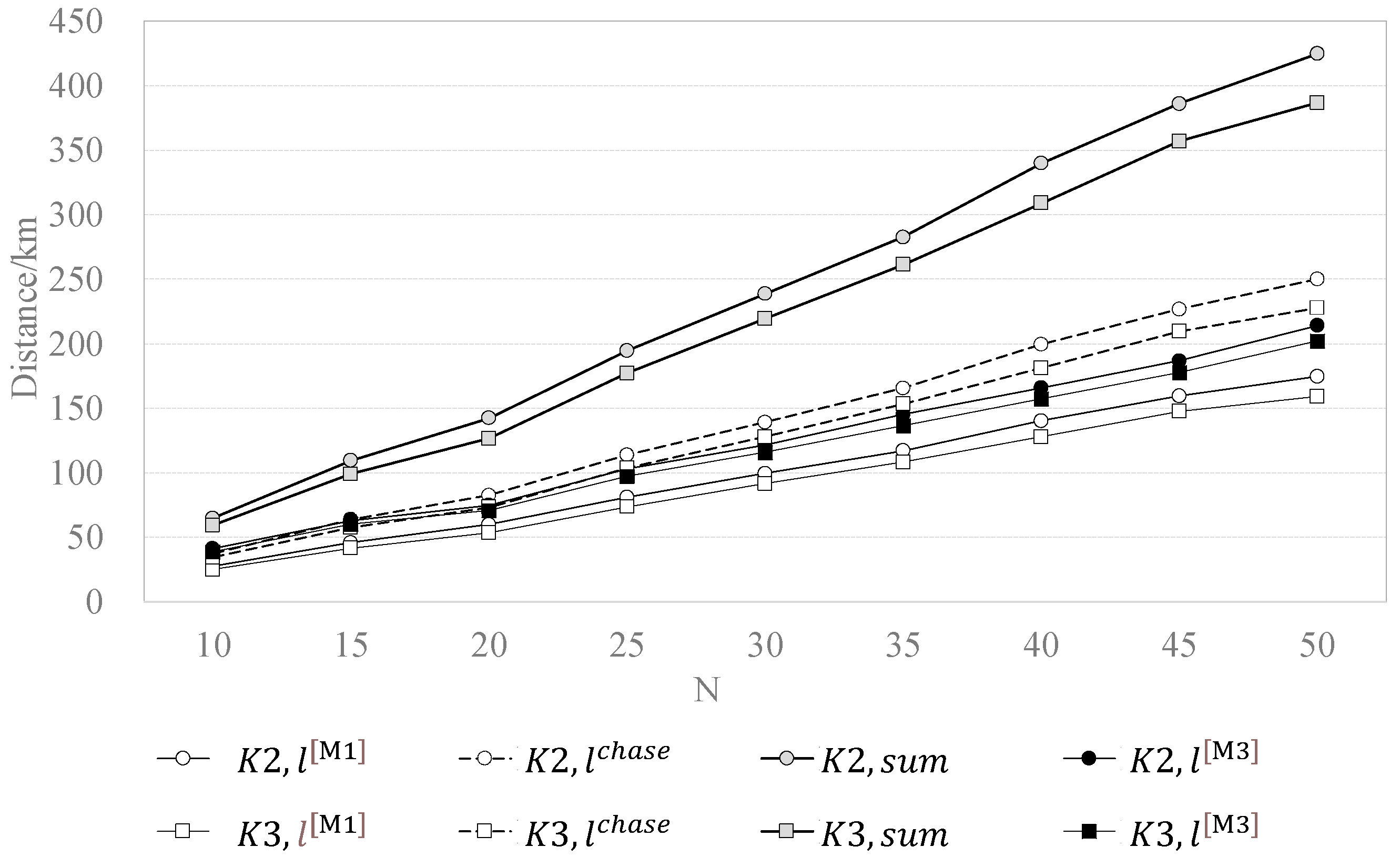
6.3.2. Comparing [M1] and [M3]

To compare the solutions of [M1] and [M3], we generate 18 datasets with varying parameters (the drone base stations and the ships, K, N) and three constant parameters (the drone’s flying speed, and two coordinate ranges, V, X, Y). Thus, the group of datasets can be denoted by “KkNnV25X20Y10”. For each dataset, we employ ten assessment metrics representing the results of [M1] and [M3]: the drones’ flying time t^[M1], chase time t^chase, and overall time; the drones’ flying distance (l^[M1]), its distances for chasing the ships (l^chase), and all the distances; and the flying time (t^[M3]) and distance (l^[M3]) for solving [M3]. Finally, we define two metrics for the ratios of flying time (t(%)) and distance (l(%)) that have been altered by using the meeting model [M2], as follows:

$$t(\%)=\frac{t^{\left[\mathrm{M}1\right]}+t^{chase}-t^{\left[\mathrm{M}3\right]}}{t^{\left[\mathrm{M}1\right]}+t^{chase}}\cdot 100,$$

$$l(\%)=\frac{l^{\left[\mathrm{M}1\right]}+l^{chase}-l^{\left[\mathrm{M}3\right]}}{l^{\left[\mathrm{M}1\right]}+l^{chase}}\cdot 100.$$

Table 5. The comparative results of solving [M1] and [M3].

K	N	t[M1]	tchase	Sum	l[M1]	lchase	Sum	t[M3]	l[M3]	t(%)	l(%)
		h	h	h	km	km	km	h	km	%	%
2	10	1.23	0.42	1.65	27.40	37.36	64.75	6.35	41.12	−7.17	36.50
2	15	1.95	0.71	2.66	45.69	63.79	109.48	9.35	62.93	2.45	42.52
2	20	2.52	0.92	3.44	59.84	82.49	142.33	11.70	74.65	5.51	47.55
2	25	3.29	1.26	4.55	80.87	113.68	194.55	15.16	102.85	7.39	47.14
2	30	4.08	1.55	5.63	99.41	139.11	238.52	17.77	121.58	12.31	49.03
2	35	4.69	1.84	6.53	117.02	165.52	282.54	20.81	145.07	11.41	48.65
2	40	5.53	2.22	7.75	140.28	199.49	339.77	23.86	165.62	14.49	51.26
2	45	6.36	2.52	8.88	159.38	226.60	385.97	27.10	186.57	15.22	51.66
2	50	6.81	2.78	9.58	174.55	250.12	424.67	30.38	213.94	11.97	49.62
3	10	1.10	0.38	1.48	25.02	34.38	59.40	5.93	38.61	−11.31	35.01
3	15	1.79	0.64	2.43	41.41	57.54	98.94	8.92	60.09	−1.93	39.27
3	20	2.26	0.81	3.07	53.27	73.23	126.50	11.14	70.76	−0.75	44.06
3	25	2.98	1.15	4.13	73.60	103.59	177.18	14.37	97.19	3.35	45.15
3	30	3.78	1.42	5.20	91.52	127.81	219.34	16.96	115.73	9.40	47.23
3	35	4.32	1.70	6.02	108.13	153.17	261.30	19.65	136.45	9.29	47.78
3	40	5.06	2.01	7.07	127.64	181.11	308.76	22.72	157.18	10.80	49.09
3	45	5.90	2.33	8.23	147.50	209.50	357.01	25.83	177.60	12.78	50.25
3	50	6.22	2.53	8.75	159.05	227.62	386.67	28.82	202.15	8.52	47.72

presents the 10 metrics of solving [M1] and [M2] for the 18 datasets. We further divide these metrics into three groups and depict them in Figure 7, Figure 8 and Figure 9. In the figures, “K = k” means the datasets have k drone base stations. In Figure 7, the values of the time-related metrics for the datasets with three drone base stations are lower than those with two. In Figure 8, we obtain similar results showing that more drones will result in shorter flying distances. Figure 7, Figure 8 and Figure 9 show that [M3] will result in shorter flying times and flying distances than [M1]. Figure 7 and Figure 8 show that the datasets with more ships will incur longer flying times and distances almost linearly. However, in Figure 9, we can see that from 45 to 50 ships, the ratios optimized by [M3] drop while they are still positive.

6.3.3. Sensitivity Analysis of Speeds via Solving [M3]

In [M1], [M2], and [M3], the drones’ and ships’ speeds are technologically and investment-dependent parameters. Increasing ships’ and drones’ speeds will generally incur higher energy costs and more emissions. Moreover, the technologies will constrain the speeds of the drones. Accelerating drones may require innovation and additional investments. In the following, we investigate the impacts of varying the drones’ and ships’ speeds on the time- and distance-related metrics, t^[M3] and l^[M3].

Table 6. Sensitivity of the ships’ speeds (V_i) for solving [M3].

K	N		t[M3]/h			l[M3]/km
		−5%	Vi/100%	5%	−5%	Vi/100%	5%
2	10	−0.73	1.76	0.71	4.28	41.12	−4.22
2	15	−0.43	2.60	0.46	4.57	62.93	−4.77
2	20	−0.63	3.25	0.61	4.37	74.65	−4.32
2	25	−0.62	4.21	0.60	4.41	102.85	−4.37
2	30	−0.76	4.94	0.74	4.26	121.58	−4.21
2	35	−0.60	5.78	0.58	4.41	145.07	−4.37
2	40	−0.57	6.63	0.55	4.44	165.62	−4.40
2	45	−0.65	7.53	0.63	4.35	186.57	−4.30
2	50	−0.71	8.44	0.69	4.30	213.94	−4.25
3	10	−0.67	1.65	0.65	4.36	38.61	−4.31
3	15	−0.56	2.48	0.61	4.41	60.09	−4.41
3	20	−0.68	3.09	0.69	4.43	70.76	−4.22
3	25	−0.67	3.99	0.68	4.35	97.19	−4.12
3	30	−0.79	4.71	0.79	4.23	115.73	−4.14
3	35	−0.67	5.46	0.68	4.24	136.45	−4.26
3	40	−0.62	6.31	0.60	4.39	157.18	−4.35
3	45	−0.68	7.18	0.68	4.28	177.60	−4.24
3	50	−0.74	8.01	0.72	4.28	202.15	−4.17

presents the sensitivity of the ships’ speeds ($V_i$) by varying them by −5% and 5%. The variances affect the time metrics t^[M3] by less than 1%, while they affect the distance metrics l^[M3] more, specifically, by about 4–5%. In

Table 7. Sensitivity of the drones’ speeds (V_k) for solving [M3].

K	N		t[M3]/h			l[M3]/km
		−5%	Vk/100%	5%	−5%	Vk/100%	5%
2	10	−0.73	1.76	0.71	4.28	41.12	−4.22
2	15	−0.43	2.60	0.46	4.57	62.93	−4.77
2	20	−0.63	3.25	0.61	4.37	74.65	−4.32
2	25	−0.62	4.21	0.60	4.41	102.85	−4.37
2	30	−0.76	4.94	0.74	4.26	121.58	−4.21
2	35	−0.60	5.78	0.58	4.41	145.07	−4.37
2	40	−0.57	6.63	0.55	4.44	165.62	−4.40
2	45	−0.65	7.53	0.63	4.35	186.57	−4.30
2	50	−0.71	8.44	0.69	4.30	213.94	−4.25
3	10	−0.67	1.65	0.65	4.36	38.61	−4.31
3	15	−0.56	2.48	0.61	4.41	60.09	−4.41
3	20	−0.68	3.09	0.69	4.43	70.76	−4.22
3	25	−0.67	3.99	0.68	4.35	97.19	−4.12
3	30	−0.79	4.71	0.79	4.23	115.73	−4.14
3	35	−0.67	5.46	0.68	4.24	136.45	−4.26
3	40	−0.62	6.31	0.60	4.39	157.18	−4.35
3	45	−0.68	7.18	0.68	4.28	177.60	−4.24
3	50	−0.74	8.01	0.72	4.28	202.15	−4.17

, we can see similar results. Accelerating the drones will optimize the drones’ flying distances more than their flying time.

6.4. Discussion and Managerial Implications

Drones are an emerging technology for the monitoring of offshore ship emissions, offering lower costs and higher flexibility and efficiency. Although there are still challenges regarding drone technologies and operation management capabilities, drones are essential for undertaking advanced technological tasks with controlled risks. Due to pollution burdens, port cities and authorities have anticipated the development of ECAs and compelled ships to use cleaner fuel in ECAs. To achieve this objective, the maritime departments must monitor the fuel usage of ships through regulations and accurate monitoring and enforcement. In this study, we formulated the ship emission detection problem as a drone-scheduling problem.

We present the following as managerial implications based on the experimental results.

(1) The drone-scheduling problem is dynamic, constituting the simultaneous movements of drones and ships. When the drones fly much faster than the ships’ movements, we can assume that the ships are waiting for the drones’ visits. However, in practice, the drones’ speed may be about three times that of the ships. The neglection of the ships’ movement is not applicable.

(2) Multiple drone base stations help decrease the flying costs and increase the coverage of the ECA, while too many stations will incur high fixed charges. Therefore, considering the endurance of the drones, we can optimize the configuration of the drone base stations.

(3) In this study, we examine the drone-scheduling problem at the operational level, while the coordination mechanisms and information systems will pre-determine operational performance. First, the drone-scheduling system must use the information from the AIS receivers to locate the ships dynamically. Second, the drone base stations must share the schedules and be organized under a top-level scheduling system. Therefore, drones can be scheduled globally. Third, the local ECA authorities should share the ship emission detection schedules and results amongst each other.

7. Conclusions

Under the background of ship emissions and their impact on port cities, we investigated the drone-scheduling problem at the operational level, especially considering multiple drone base stations for long ECA ranges. We conducted this research after examining the related studies, technologies, and applications. Considering the simultaneous movements of drones and ships, we devised models for immobile and mobile ships. The two models can share the same structure while changing the traveling time matrix through a meeting model between a drone and a ship. The models were demonstrated and investigated through experiments.

The research in the present study can be extended in future studies in terms of the following aspects. First, we assume that each ship has a fixed moving direction and velocity, while the ships may change their directions slowly in practical situations. We can obtain the dynamics of the moving directions and speeds through AIS data. Second, the drones are presumed to start from the drone base stations and return after a one-ship task. When endurance permits, a drone can perform several detection tasks. By extending the devised models, we can conduct new studies to render the solutions suitable for more practical situations and support ship emission detection. The drones used in emission detection tasks will also face security problems and attacks [42,43], so it is difficult to consider safety with respect to the scheduling of drones by incorporating additional sensor information to identify insecure areas in the ECAs. The drones can be taken as edge computing devices, and their data should be collected and managed in secure cloud systems [44,45]. It is beneficial to consider the innovation of drone technology and its impacts on applications.

References

1. Liu, J.H.; Duru, O.; Law, A.W.K. Assessment of atmospheric pollutant emissions with maritime energy strategies using bayesian simulations and time series forecasting. Environ. Pollut. 2021, 270, 116068. [Google Scholar] [CrossRef]
2. Bacalja, B.; Krcum, M.; Sliskovic, M. A Line Ship Emissions while Manoeuvring and Hotelling-A Case Study of Port Split. J. Mar. Sci. Eng. 2020, 8, 953. [Google Scholar] [CrossRef]
3. Fan, L.X.; Gu, B.M.; Luo, M.F. A cost-benefit analysis of fuel-switching vs. hybrid scrubber installation: A container route through the Chinese SECA case. Transp. Policy 2020, 99, 336–344. [Google Scholar] [CrossRef]
4. Huang, L.; Wen, Y.Q.; Zhang, Y.M.; Zhou, C.H.; Zhang, F.; Yang, T.T. Dynamic calculation of ship exhaust emissions based on real-time AIS data. Transp. Res. Part D-Transp. Environ. 2020, 80, 102277. [Google Scholar] [CrossRef]
5. Anand, A.; Wei, P.; Gali, N.K.; Sun, L.; Yang, F.H.; Westerdahl, D.; Zhang, Q.; Deng, Z.Q.; Wang, Y.; Liu, D.G.; et al. Protocol development for real-time ship fuel sulfur content determination using drone based plume sniffing microsensor system. Sci. Total Environ. 2020, 744, 140885. [Google Scholar] [CrossRef]
6. Tovar, B.; Tichavska, M. Environmental cost and eco-efficiency from vessel emissions under diverse SOx regulatory frameworks: A special focus on passenger port hubs. Transp. Res. Part D-Transp. Environ. 2019, 69, 1–12. [Google Scholar] [CrossRef]
7. Sun, Y.L.; Yang, L.X.; Zheng, J.F. Emission control areas: More or fewer? Transp. Res. Part D-Transp. Environ. 2020, 84, 102349. [Google Scholar] [CrossRef]
8. Chang, Y.T.; Park, H.; Lee, S.; Kim, E. Have Emission Control Areas (ECAs) harmed port efficiency in Europe? Transp. Res. Part D-Transp. Environ. 2018, 58, 39–53. [Google Scholar] [CrossRef]
9. Zhen, L.; Li, M.; Hu, Z.; Lv, W.Y.; Zhao, X. The effects of emission control area regulations on cruise shipping. Transp. Res. Part D-Transp. Environ. 2018, 62, 47–63. [Google Scholar] [CrossRef]
10. Chen, L.Y.; Yip, T.L.; Mou, J.M. Provision of Emission Control Area and the impact on shipping route choice and ship emissions. Transp. Res. Part D-Transp. Environ. 2018, 58, 280–291. [Google Scholar] [CrossRef]
11. Carr, E.W.; Corbett, J.J. Ship Compliance in Emission Control Areas: Technology Costs and Policy Instruments. Environ. Sci. Technol. 2015, 49, 9584–9591. [Google Scholar] [CrossRef] [PubMed]
12. Ma, W.H.; Hao, S.F.; Ma, D.F.; Wang, D.H.; Jin, S.; Qu, F.Z. Scheduling decision model of liner shipping considering emission control areas regulations. Appl. Ocean. Res. 2021, 106, 102416. [Google Scholar] [CrossRef]
13. Jiang, B.; Wang, X.Q.; Xue, H.L.; Li, J.; Gong, Y. An evolutionary game model analysis on emission control areas in China. Mar. Policy 2020, 118, 104010. [Google Scholar] [CrossRef]
14. Cariou, P.; Cheaitou, A.; Larbi, R.; Hamdan, S. Liner shipping network design with emission control areas: A genetic algorithm-based approach. Transp. Res. Part D-Transp. Environ. 2018, 63, 604–621. [Google Scholar] [CrossRef]
15. Abioye, O.F.; Dulebenets, M.A.; Pasha, J.; Kavoosi, M. A Vessel Schedule Recovery Problem at the Liner Shipping Route with Emission Control Areas. Energies 2019, 12, 2380. [Google Scholar] [CrossRef] [Green Version]
16. Tian, X.C.; Yan, R.; Qi, J.W.; Zhuge, D.; Wang, H. A Bi-Level Programming Model for China’s Marine Domestic Emission Control Area Design. Sustainability 2022, 14, 3562. [Google Scholar] [CrossRef]
17. Dong, G.; Lee, P.T.W. Environmental effects of emission control areas and reduced speed zones on container ship operation. J. Clean. Prod. 2020, 274, 122582. [Google Scholar] [CrossRef]
18. Ma, W.H.; Lu, T.F.; Ma, D.F.; Wang, D.H.; Qu, F.Z. Ship route and speed multi-objective optimization considering weather conditions and emission control area regulations. Marit. Policy Manag. 2021, 48, 1053–1068. [Google Scholar] [CrossRef]
19. Li, L.Y.; Pan, Y.; Gao, S.X.; Yang, W.G. An innovative model to design extreme emission control areas (ECAs) by considering ship?s evasion strategy. Ocean. Coast. Manag. 2022, 227, 106289. [Google Scholar] [CrossRef]
20. Sheng, D.; Meng, Q.; Li, Z.C. Optimal vessel speed and fleet size for industrial shipping services under the emission control area regulation. Transp. Res. Part C-Emerg. Technol. 2019, 105, 37–53. [Google Scholar] [CrossRef]
21. Zhang, Q.; Liu, H.Y.; Wan, Z. Evaluation on the effectiveness of ship emission control area policy: Heterogeneity detection with the regression discontinuity method. Environ. Impact Assess. Rev. 2022, 94, 106747. [Google Scholar] [CrossRef]
22. Wang, X.; Pang, Y.; Wang, H.; Shen, C.Q.; Wang, X. Emission Control in River Network System of the Taihu Basin for Water Quality Assurance of Water Environmentally Sensitive Areas. Sustainability 2017, 9, 301. [Google Scholar] [CrossRef] [Green Version]
23. Cui, H.; Notteboom, T. Modelling emission control taxes in port areas and port privatization levels in port competition and co-operation sub-games. Transp. Res. Part D-Transp. Environ. 2017, 56, 110–128. [Google Scholar] [CrossRef]
24. Wan, Z.; Zhou, X.J.; Zhang, Q.; Chen, J.H. Do ship emission control areas in China reduce sulfur dioxide concentrations in local air? A study on causal effect using the difference-in-difference model. Mar. Pollut. Bull. 2019, 149, 110506. [Google Scholar] [CrossRef]
25. Kuzniar, M.; Pawlak, M.; Orkisz, M. Comparison of Pollutants Emission for Hybrid Aircraft with Traditional and Multi-Propeller Distributed Propulsion. Sustainability 2022, 14, 15076. [Google Scholar] [CrossRef]
26. Yi, W.; Sutrisna, M. Drone scheduling for construction site surveillance. Comput.-Aided Civ. Infrastruct. Eng. 2021, 36, 3–13. [Google Scholar] [CrossRef]
27. Hassija, V.; Saxena, V.; Chamola, V. Scheduling drone charging for multi-drone network based on consensus time-stamp and game theory. Comput. Commun. 2020, 149, 51–61. [Google Scholar] [CrossRef]
28. Torabbeigi, M.; Lim, G.J.; Kim, S.J. Drone Delivery Scheduling Optimization Considering Payload-induced Battery Consumption Rates. J. Intell. Robot. Syst. 2020, 97, 471–487. [Google Scholar] [CrossRef]
29. Dell’Amico, M.; Montemanni, R.; Novellani, S. Matheuristic algorithms for the parallel drone scheduling traveling salesman problem. Ann. Oper. Res. 2020, 289, 211–226. [Google Scholar] [CrossRef] [Green Version]
30. Chowdhery, A.; Jamieson, K. Aerial Channel Prediction and User Scheduling in Mobile Drone Hotspots. IEEE-Acm Trans. Netw. 2018, 26, 2679–2692. [Google Scholar] [CrossRef]
31. Torabbeigi, M.; Lim, G.J.; Ahmadian, N.; Kim, S.J. An Optimization Approach to Minimize the Expected Loss of Demand Considering Drone Failures in Drone Delivery Scheduling. J. Intell. Robot. Syst. 2021, 102, 22. [Google Scholar] [CrossRef]
32. Kim, S.J.; Lim, G.J.; Cho, J. Drone flight scheduling under uncertainty on battery duration and air temperature. Comput. Ind. Eng. 2018, 117, 291–302. [Google Scholar] [CrossRef]
33. Kim, S.J.; Lim, G.J. A Hybrid Battery Charging Approach for Drone-Aided Border Surveillance Scheduling. Drones 2018, 2, 38. [Google Scholar] [CrossRef] [Green Version]
34. Park, H.J.; Mirjalili, R.; Cote, M.J.; Lim, G.J. Scheduling Diagnostic Testing Kit Deliveries with the Mothership and Drone Routing Problem. J. Intell. Robot. Syst. 2022, 105, 38. [Google Scholar] [CrossRef] [PubMed]
35. Torky, M.; El-Dosuky, M.; Goda, E.; Snasel, V.; Hassanien, A.E. Scheduling and Securing Drone Charging System Using Particle Swarm Optimization and Blockchain Technology. Drones 2022, 6, 237. [Google Scholar] [CrossRef]
36. Gentili, M.; Mirchandani, P.B.; Agnetis, A.; Ghelichi, Z. Locating platforms and scheduling a fleet of drones for emergency delivery of perishable items. Comput. Ind. Eng. 2022, 168, 108057. [Google Scholar] [CrossRef]
37. Jung, H.; Kim, J. Drone scheduling model for delivering small parcels to remote islands considering wind direction and speed. Comput. Ind. Eng. 2022, 163, 107784. [Google Scholar] [CrossRef]
38. Salama, M.R.; Srinivas, S. Collaborative truck multi-drone routing and scheduling problem: Package delivery with flexible launch and recovery sites. Transp. Res. Part E-Logist. Transp. Rev. 2022, 164, 102788. [Google Scholar] [CrossRef]
39. Su, Y.; Wang, S.J.; Cheng, Q.N.; Qiu, Y.H. Buffer evaluation model and scheduling strategy for video streaming services in 5G-powered drone using machine learning. Eurasip J. Image Video Process. 2021, 2021, 29. [Google Scholar] [CrossRef]
40. Liu, C.; Chen, H.P.; Li, X.P.; Liu, Z.Y. A scheduling decision support model for minimizing the number of drones with dynamic package arrivals and personalized deadlines. Expert Syst. Appl. 2021, 167, 114157. [Google Scholar] [CrossRef]
41. Asadi, A.; Pinkley, S.N. A Monotone Approximate Dynamic Programming Approach for the Stochastic Scheduling, Allocation, and Inventory Replenishment Problem: Applications to Drone and Electric Vehicle Battery Swap Stations. Transp. Sci. 2022, 56, 1085–1110. [Google Scholar] [CrossRef]
42. Krichen, M.; Adoni, W.Y.H.; Mihoub, A.; Alzahrani, M.Y.; Nahhal, T. Security Challenges for Drone Communications: Possible Threats, Attacks and Countermeasures. In Proceedings of the 2nd International Conference of Smart Systems and Emerging Technologies (SMARTTECH), Riyadh, Saudi Arabia, 9–11 May 2022; pp. 184–189. [Google Scholar]
43. Bunse, C.; Plotz, S. Security Analysis of Drone Communication Protocols. In Engineering Secure Software and Systems. ESSoS 2018. Lecture Notes in Computer Science; Payer, M., Rashid, A., Such, J., Eds.; Springer: Cham, Switzerland, 2018; Volume 10953. [Google Scholar]
44. Yang, H.; Yuan, J.; Li, C.; Zhao, G.; Sun, Z.; Yao, Q.; Bao, B.; Vasilakos, A.V.; Zhang, J. BrainIoT: Brain-Like Productive Services Provisioning With Federated Learning in Industrial IoT. IEEE Internet Things J. 2022, 9, 2014–2024. [Google Scholar] [CrossRef]
45. Li, C.; Yang, H.; Sun, Z.; Yao, Q.; Bao, B.; Zhang, J.; Vasilakos, A.V. Federated Hierarchical Trust-Based Interaction Scheme for Cross-Domain Industrial IoT. IEEE Internet Things J. 2023, 10, 447–457. [Google Scholar] [CrossRef]
Figure 1. A systematic scheme of the proposed models and solution methods.
Drones 07 00158 g001
Figure 2. A conceptual diagram of drone routing for emission detection.
Drones 07 00158 g002
Figure 3. A meeting model for a drone and directional mobile ship.
Drones 07 00158 g003
Figure 4. A conceptual diagram of drone routing for emission detection.
Drones 07 00158 g004
Figure 5. Background diagram for dataset generation.
Drones 07 00158 g005
Figure 6. Demonstration of the solutions with and without the meeting model [M2].
Drones 07 00158 g006
Figure 7. The time-related metrics for the results of solving [M1] and [M3].
Drones 07 00158 g007
Figure 8. Distance-related metrics for the results of solving [M1] and [M3].
Drones 07 00158 g008
Figure 9. Reduced ratios of time- and distance-related metrics for solving [M1] and [M3].
Drones 07 00158 g009