Article

Attitude Control of a Hypersonic Glide Vehicle Based on Reduced-Order Modeling and NESO-Assisted Backstepping Variable Structure Control

1
College of Engineering, China Agricultural University, Beijing 100083, China
2
Key Laboratory of Spatial-Temporal Big Data Analysis and Application of Natural Resources in Megacities, MNR, Shanghai 200063, China
3
Key Laboratory of Urban Land Resources Monitoring and Simulation, Ministry of Natural Resources, Shenzhen 518000, China
4
State Key Laboratory of Virtual Reality Technology and Systems, Beihang University, Beijing 100191, China
5
Key Laboratory of Smart Agricultural Technology in Tropical South China, Ministry of Agriculture and Rural Affairs, Guangzhou 510642, China
6
Jiangsu Province and Education Ministry Co-Sponsored Synergistic Innovation Center of Modern Agricultural Equipment, Jiangsu University, Zhenjiang 212013, China
*
Author to whom correspondence should be addressed.
Drones 2023, 7(2), 119; https://doi.org/10.3390/drones7020119
Submission received: 6 January 2023 / Revised: 2 February 2023 / Accepted: 3 February 2023 / Published: 8 February 2023

Abstract

:
Aiming at solving the control problem caused by the large-scale change of the Hypersonic Glide Vehicle (HGV) parameters, this paper proposes a design method of backstepping variable structure attitude controller based on Nonlinear Extended State Observer (NESO), with the characteristics of HGV model and the idea of uncertainty estimation and compensation associated. Firstly, the design of the second-order NESO is studied. Due to the large number of NESO parameters, a systematic method for determining the second-order NESO parameters is given in this paper, and the stability of the observer is proved completely using the piecewise Lyapunov analysis. Then, the NESO-assisted backstepping variable structure attitude controller employs the reduced-order modeling idea to decompose the whole system design problem into two first-order subsystem design problem, and classifies the nonlinear dynamic changes caused by the large-scale changes of the aircraft parameters into the aggregated uncertain terms of the two subsystems. The simulation results show that the backstepping attitude controller based on NESO can realize the stable and accurate tracking of the flight attitude when the aircraft parameters change in a large range.

1. Introduction

A hypersonic vehicle is a new project of cutting-edge technology being developed in this century whose flying height can be 20–100 km above the ground in the atmospheric space. It is an undeveloped near space area which is located below the orbit of low-orbit satellites and above the flight height of general aircraft, including the stratosphere, mesosphere, and part of the thermosphere [1]. Owing to its high speed, small target cross section, and strong maneuverability, the hypersonic vehicle is a great threat to missile defense systems which have been unable to intercept. This will change the existing mode of warfare to some extent [2]. Considering the characteristics of hypersonic vehicle that the aerodynamic characteristics and thermal characteristics change dramatically [3], the attitude control during reentry glide terminal guidance is difficult due to the complex aerodynamic characteristics, high nonlinearity of system model.
The reentry gliding of Hypersonic Glide Vehicle (HGV) is a long-time and long-span flight process, in which the vehicle’s altitude and speed will undergo a wide range of changes [4,5]. Both of them have a significant impact on vehicle parameters such as atmospheric density and aerodynamic parameters. This impact leads to a wide range of changes in vehicle parameters during the flight process and makes the vehicle’s dynamic characteristics at the beginning and end of the glide greatly different [6]. Therefore, to realize the robust control of HGV flight attitude, it is crucial to adapt to the large-scale changes of vehicle parameters.
Regarding the nonlinear dynamic change of vehicle caused by the change of vehicle parameters and the unknown external disturbance as an aggregated uncertainty, the effects of the large-scale changes in vehicle parameters can be overcome through real-time estimation of the aggregated uncertainty and cancellation in the control law.
The idea of extended state observer is to estimate the state and uncertainty of the system by expanding the uncertainty into a new state variable, and then establishing a state observer for the extended system. Gao et al. studied the stable convergence characteristics [7,8] and digital implementation [9] of the Linear Extended State Observer (LESO). Han proposed the Nonlinear Extended State Observer (NESO) [10] with the advantages of non-smooth and nonlinear functions, which has faster convergence speed and better estimation accuracy than the LESO. Huang et al. analyzed the convergence characteristics and observation error accuracy of the second-order NESO by using the self-stable region method [11,12,13] and the piecewise smooth Lyapunov function method [14]. Pu et al. proposed an Adaptive Extended State Observer (AESO) to nonlinear disturbed systems, applied it to a MIMO hypersonic vehicle, and compared results with LESO and NESO [15]. Due to the large number of NESO parameters and complex relationships, no systematic method for determining the parameters of observers has been given in previous literature, and the stability characteristics of the linear approximation region of the fal function have been ignored. In this paper, aiming at the above two problems, the Lyapunov method is used to completely discuss the stability of the second-order NESO and to solve the design problem of the observer parameters.
HGV’s aggregated uncertainties can be divided into two types: matching and non-matching, both of which meet the generalized matching conditions. For the control of nonlinear systems with both matching and non-matching uncertainties, emerging nonlinear control methods such as Sliding Mode Control (SMC) and backstepping have been favored by many researchers and engineers. Sliding mode variable structure control is essentially a kind of nonlinear robust control method, and its main advantage is that the system response is not sensitive to the uncertainty and disturbance of the model [16,17]. The nonlinear adaptive sliding mode controllers were proposed subject to uncertainties, disturbances and faults [18,19]. Based on the integral sliding mode control, an adaptive sliding controller was designed to overcome the effect of actuator faults and unknown disturbances [20]. Jiang et al. [21] and Ahmed et al. [22] used a method of sliding mode control combing with observer or adaptive control law to deal with system uncertainty and external disturbance for different robot systems.
However, when the change of aircraft parameters is too large and exceeds the tolerance range of the variable structure switching gain, the stable control of flight attitude cannot be achieved by the sliding mode variable structure attitude control.
In past few years, the intelligent control methods have been applied in more complex problems in the control area, especially some nonlinear models, and the requirement becomes more accurate. For the HGV, studies on the same type of control problems may have different methods to achieve the ideal control effect according to the specific problems to be solved. This paper briefly combs a great deal of articles about the control problems of HGV in recent years and classifies them according to the types of control problems; the results are shown in Table 1.
It can be clearly seen from the above table that researchers have mainly spent their energy on HGV attitude control, fault-tolerant control, trajectory tracking control, disturbance rejection control, optimal control, and formation control in recent years. Among them, the attitude control of HGV is the most important. This is also very reasonable, because all the in-depth and complex research on hypersonic vehicle is based on the stable and accurate control of its attitude.
In order to solve the attitude control problems caused by the large-scale change of parameters during the flight of the HGV, as well as the uncertainty of unknown disturbances during the flight, this paper proposes to combine the controller with NSEOs which can estimate the state and uncertainties of the system and use backstepping variable structure control for HGV attitude control. The innovations are summarized as follows:
(1)
According to the quality of the estimation of the uncertainties by the Extended State Observer (ESO), the corresponding design idea of the improved backstepping variable structure controller is proposed in this paper. The design of the whole system is divided into two first-order subsystems, and the pseudo-control filter is introduced while the error signal is corrected ensuring the adaptability of the attitude controller to the large-scale variation of vehicle’s parameters.
(2)
For unknown system states and unpredictable disturbances of two first-order subsystems, two sets of second-order NESO are designed to estimate these two kinds of uncertainties, respectively, and those two nonlinear dynamic changes are regarded as an aggregate uncertainty. Especially, a systematic method for determining those two second-order NESOs parameters is designed in this paper, and the stability of the observer is proven completely using the piecewise Lyapunov analysis. Aiming at avoiding complicated analytical operations, this paper proposes an improved backstepping control method by introducing the pseudo-control filter and the correcting the error signal assisted with the NESO.
The remainder is organized as follows. In Section 2, the second-order NSEO is designed, and the parameters are designed to make the observer have smaller convergence region and higher accuracy. Based on the observation results of NESO, the traditional backstepping control method is improved, and the pseudo-control filter is introduced to carry out the backstepping variable structure attitude control of HGV, which requires only a small control gain to achieve high tracking accuracy in Section 3. In Section 4, a series of simulation experiments are carried out on the HGV attitude control theory which combines NESO with backstepping variable structure control, and the experimental results are fully analyzed. Finally, Section 5 presents the conclusions of this work.

2. Extended State Observer

According to the observation purpose of the observer, the observers can be divided into state observers and disturbance observers. The former is used to observe the state of the system: for linear systems, there are Luenberger observers and Kalman filters; for nonlinear systems, there are high-gain observers, extended Kalman filters, and nonlinear observers based on Lyapunov method or differential geometry method. The latter equates the difference between the actual object and the nominal model output caused by external interference and changes in model parameters to the control input and makes an observation on it. For linear systems, there are unknown input observers and internal model observers; for nonlinear systems, there are sliding mode disturbance observers, harmonic disturbance observers, and intelligent disturbance observers.
In recent years, the observers that can realize both state estimation and disturbance estimation have attracted researchers’ interest. ESO is such a novel observer which was proposed by Han [7]. It cannot only observe all states of the system, but also observe the uncertainty and external disturbance of the system.

2.1. Scenario Design

Consider the following n-order SISO affine nonlinear system:
x ˙ 1 = x 2 x ˙ 2 = x 3 x ˙ n 1 = x n x ˙ n = f ( x 1 , x 2 , , x n ) + b u + w ( t ) y = x 1
where uncertain nonlinear function:
f ( x 1 , x 2 , , x n ) = f 0 ( x 1 , x 2 , , x n ) + Δ f ( x 1 , x 2 , , x n ) . f 0 ( x 1 , x 2 , , x n ) is the nominal known part, Δ f ( x 1 , x 2 , , x n ) is the uncertain part, w ( t ) is the unknown external disturbance, b = b 0 + ( b b 0 ) , and its nominal value is b 0 .
Summarize all kinds of uncertain factors of the system and obtain the aggregated uncertainty:
d = Δ f ( x 1 , x 2 , , x n ) + w ( t ) + ( b b 0 ) u
Then, by expanding the aggregated uncertainty d into a new state variable x n + 1 , the augmented system can be obtained and the extended state observer designed for it is shown as follows:
x ˜ 1 = z 1 y z ˙ 1 = z 2 β 1 f c 1 ( x ˜ 1 ) z ˙ 2 = z 3 β 2 f c 2 ( x ˜ 1 ) z ˙ n 1 = z n β n 1 f c n 1 ( x ˜ 1 ) z ˙ n = z n + 1 β n f c n ( x ˜ 1 ) + f 0 ( x 1 , x 2 , , x n ) + b 0 u z ˙ n + 1 = β n + 1 f c ( n + 1 ) ( x ˜ 1 )
where β 1 , β 2 , β n + 1 are gain parameters of the observer, f c i ( x ˜ ) is the output error function ( i = 1 , 2 , , n + 1 ), x n + 1 = d and x ˙ n + 1 = v ( t ) .
From Equation (4), the equation of observation error can be obtained:
x ˜ i = z i x i x ˜ ˙ 1 = x ˜ 2 β 1 f c 1 ( x ˜ 1 ) x ˜ ˙ 2 = x ˜ 3 β 2 f c 2 ( x ˜ 1 ) x ˜ ˙ n 1 = x ˜ n β n 1 f c n 1 ( x ˜ 1 ) x ˜ ˙ n = x ˜ n + 1 β n f c n ( x ˜ 1 ) x ˜ ˙ n + 1 = β n + 1 f c ( n + 1 ) ( x ˜ 1 ) v ( t )
As long as the change rate of aggregated uncertainty d ˙ = v ( t ) is bounded, and the output error function f c i ( x ˜ ) , i = 1 , 2 , , n + 1 satisfies the condition:
x ˜ 1 f c i ( x ˜ ˙ 1 ) > 0 , x ˜ ˙ 1 0 , f c i ( 0 ) = 0
Then, system (4) can reach a stable state at the origin by carefully designing gain parameters β 1 , β 2 , β n + 1 > 0 .
The states of the observer (3) are the output, the derivatives of the output, and the estimation of the aggregated uncertainty:
z 1 y z 2 y ( 1 ) z n 1 y ( n 2 ) z n y ( n 1 ) z n + 1 d
If the output error function f c i ( e 1 ) is a linear function, Equation (3) is a LESO, and if the output error function f c i ( e 1 ) is a nonlinear function, Equation (3) is a NESO.

2.2. Analysis and Design of Second-Oeder NESO

In this section, the Lyapunov method is used to completely discuss the stability of the second-order NESO and to solve the design problem of the observer parameters.
Theorem 1. 
For the first-order uncertain nonlinear system
x ˙ = f 0 ( x ) + b 0 u + d
Assuming that the derivative of the uncertainty is bounded to d ˙ d ¯ v , the second-order NESO is designed as follows:
x ˜ 1 = z 1 x x ˜ 2 = z 2 d z ˙ 1 = f 0 ( x ) + b 0 u + z 2 β 1 x ˜ 1 z ˙ 2 = β 2 f a l ( x ˜ 1 , a , δ )
f a l ( x ˜ 1 , a , δ ) = x ˜ 1 a sgn ( x ˜ 1 ) x ˜ 1 > δ x ˜ 1 / δ 1 a x ˜ 1 δ
If
1 2 β 1 2 > β 2 > d ¯ v
then a = a and δ are chosen, where a is the optimal index parameter and δ is the parameter in the linear approximation area, so that
r 0 = d ¯ v β 2 1 a = 2 d ¯ v β 1 2 + 2 β 2 β 1 2 1 1 a a a 1 a ( 1 a )
2 β 2 β 1 2 δ a δ 2 d ¯ v β 1 2 + 2 β 2 β 1 2 1 1 a a a 1 a ( 1 a )
Then, there are observer errors x ˜ 1 , x ˜ 2 , which can converge to the following area:
G 0 = { ( x ˜ 1 , x ˜ 2 ) x ˜ 1 d ¯ v / β 2 1 a , x ˜ 2 β 1 d ¯ v / β 2 1 a }
Proof. 
The observation error equation is:
x ˜ ˙ 1 = x ˜ 2 β 1 x ˜ 1 x ˜ ˙ 2 = d ˙ β 2 f a l ( x ˜ 1 , a , δ )
The x ˜ 1 , x ˜ 2 plane is divided into five regions: G0, G1, G2, G3, G4, as shown in Figure 1.
For G j , j = 1 , 2 , 3 , 4 , we design the discontinuous piecewise smooth Lyapunov positive definite function V j ( x ˜ 1 , x ˜ 2 ) :
V j x ˜ 1 , x ˜ 2 = β 1 2 x ˜ 1 r 0 , x ˜ 1 , x ˜ 2 G 1 = x ˜ 1 , x ˜ 2 x ˜ 1 > r 0 , 0 x ˜ 2 < β 1 x ˜ 1 x ˜ 2 β 1 x ˜ 1 , x ˜ 1 , x ˜ 2 G 2 = x ˜ 1 , x ˜ 2 x ˜ 2 > 0 , x ˜ 2 β 1 2 x ˜ 1 + r 0 1 , x ˜ 2 β 1 x ˜ 1 β 1 2 x ˜ 1 + r 0 , x ˜ 1 , x ˜ 2 G 3 = x ˜ 1 , x ˜ 2 x ˜ 1 < r 0 , 0 x ˜ 2 > β 1 x ˜ 1 x ˜ 2 + β 1 x ˜ 1 , x ˜ 1 , x ˜ 2 G 4 = x ˜ 1 , x ˜ 2 x ˜ 2 < 0 , x ˜ 2 β 1 2 x ˜ 1 r 0 , x ˜ 2 β 1 x ˜ 1
The condition that the observation error x ˜ 1 , x ˜ 2 can converge to the region G 0 is that d V j ( x ˜ 1 , x ˜ 2 ) d t < 0 holds in every G j , j = 1 , 2 , 3 , 4 .
Next, the analysis is carried out in different regions:
(1) When ( x ˜ 1 , x ˜ 2 ) G 1 , x ˜ 2 < β 1 x ˜ 1 .
d V 1 ( x ˜ 1 , x ˜ 2 ) d t = β 1 2 x ˜ ˙ 1 = β 1 2 ( x ˜ 2 β 1 x ˜ 1 ) < 0
(2) When ( x ˜ 1 , x ˜ 2 ) G 2 , there are two cases for discussion:
x ˜ 1 > δ
The observation error dynamics equation is:
x ˜ ˙ 1 = x ˜ 2 β 1 x ˜ 1 x ˜ ˙ 2 = d ˙ β 2 x ˜ 1 a sgn ( x ˜ 1 )
d V 2 ( x ˜ 1 , x ˜ 2 ) d t = x ˜ ˙ 2 β 1 x ˜ ˙ 1 = d ˙ β 2 x ˜ 1 a sgn ( x ˜ 1 ) β 1 ( x ˜ 2 β 1 x ˜ 1 )
Assuming the derivative of uncertainty is bounded to d ˙ d ¯ v , then
d V 2 ( x ˜ 1 , x ˜ 2 ) d t d ¯ v β 2 x ˜ 1 a sgn ( x ˜ 1 ) β 1 ( x ˜ 2 β 1 x ˜ 1 )
In G 2 , x ˜ 2 can be expressed as
x ˜ 2 = β 1 2 ( x ˜ 1 + r ) , r r 0 , x ˜ 1 r
Substituting Equation (18) into Equation (17), we have
d V 2 ( x ˜ 1 , x ˜ 2 ) d t d ¯ v β 2 x ˜ 1 a sgn ( x ˜ 1 ) β 1 β 1 2 ( x ˜ 1 + r ) β 1 x ˜ 1 = d ¯ v β 2 x ˜ 1 a sgn ( x ˜ 1 ) + β 1 2 2 ( x ˜ 1 r )
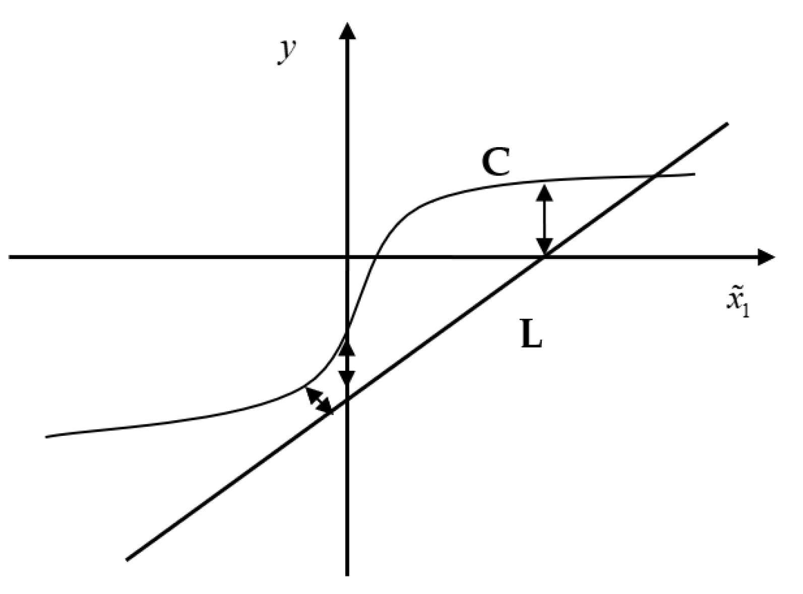
Denote the equation of line L is y = β 1 2 2 ( x ˜ 1 r ) , the equation of curve C is y = d ¯ v + β 2 x ˜ 1 a sgn ( x ˜ 1 ) , and the shape is convex and concave. If it is within G 2 and the curve C is above the straight line L, then there is d V 2 ( x ˜ 1 , x ˜ 2 ) d t < 0 .
As can be seen from Figure 2, if the corresponding three points on the curve C and the line L meet:
d ¯ v + β 2 r a > 0 d ¯ v > β 1 2 2 r d ¯ v β 2 x ˜ 1 , min a > β 1 2 2 ( x ˜ 1 , min r ) ,
then the curve C is above the line L. Among them, when r x ˜ 1 < 0 , x ˜ 1 , min = ( 2 a β 2 β 1 2 ) 1 1 a is x ˜ 1 which minimizes the difference between the curve C and the straight line L.
From Equation (20), if it meets:
r > r 0 , r 0 = max β 2 d ¯ v 1 a , 2 d ¯ v β 1 2 + 2 β 2 β 1 2 1 1 a a a 1 a ( 1 a ) ,
then d V 2 ( x ˜ 1 , x ˜ 2 ) d t < 0 holds.
x ˜ 1 δ
At this time, the observation error dynamics equations are:
x ˜ ˙ 1 = x ˜ 2 β 1 x ˜ 1 x ˜ ˙ 2 = d ˙ β 2 x ˜ 1 / δ 1 a
d V 2 ( x ˜ 1 , x ˜ 2 ) d t = x ˜ ˙ 2 β 1 x ˜ ˙ 1 = d ˙ β 2 x ˜ 1 / δ 1 a β 1 ( x ˜ 2 β 1 x ˜ 1 ) d ¯ v β 2 x ˜ 1 / δ 1 a + β 1 2 2 ( x ˜ 1 r )
Denote the equation of line L is y = β 1 2 2 ( x ˜ 1 r ) and the equation of line M is y = d ¯ v + β 2 x ˜ 1 / δ 1 a . If r meets the following equation in G 2 :
d ¯ v β 2 δ a > β 1 2 2 ( δ r ) d ¯ v + β 2 δ a > β 1 2 2 ( δ r ) ,
then line M is above L.
From Equation (24), when
r > 2 d ¯ v β 1 2 + 2 β 2 β 1 2 δ a δ ,
d V 2 ( x ˜ 1 , x ˜ 2 ) d t < 0 holds.
(3) Because G 1 and G 3 are symmetrical, G 2 and G 4 are symmetrical, the result obtained when ( x ˜ 1 , x ˜ 2 ) G 3 is the same as ( x ˜ 1 , x ˜ 2 ) G 1 , and the result obtained when ( x ˜ 1 , x ˜ 2 ) G 4 is the same as ( x ˜ 1 , x ˜ 2 ) G 2 .
In sum, there are the following conclusions.
When
r > r 0 , r 0 = max β 2 d ¯ v 1 a , 2 d ¯ v β 1 2 + 2 β 2 β 1 2 1 1 a a a 1 a ( 1 a ) , 2 d ¯ v β 1 2 + 2 β 2 β 1 2 δ a δ
d V i ( x ˜ 1 , x ˜ 2 ) d t < 0 holds.
If parameter d ¯ v < β 2 < 1 2 β 1 2 , then:
β 2 d ¯ v < 1 , 2 β 2 β 1 2 < 1 .
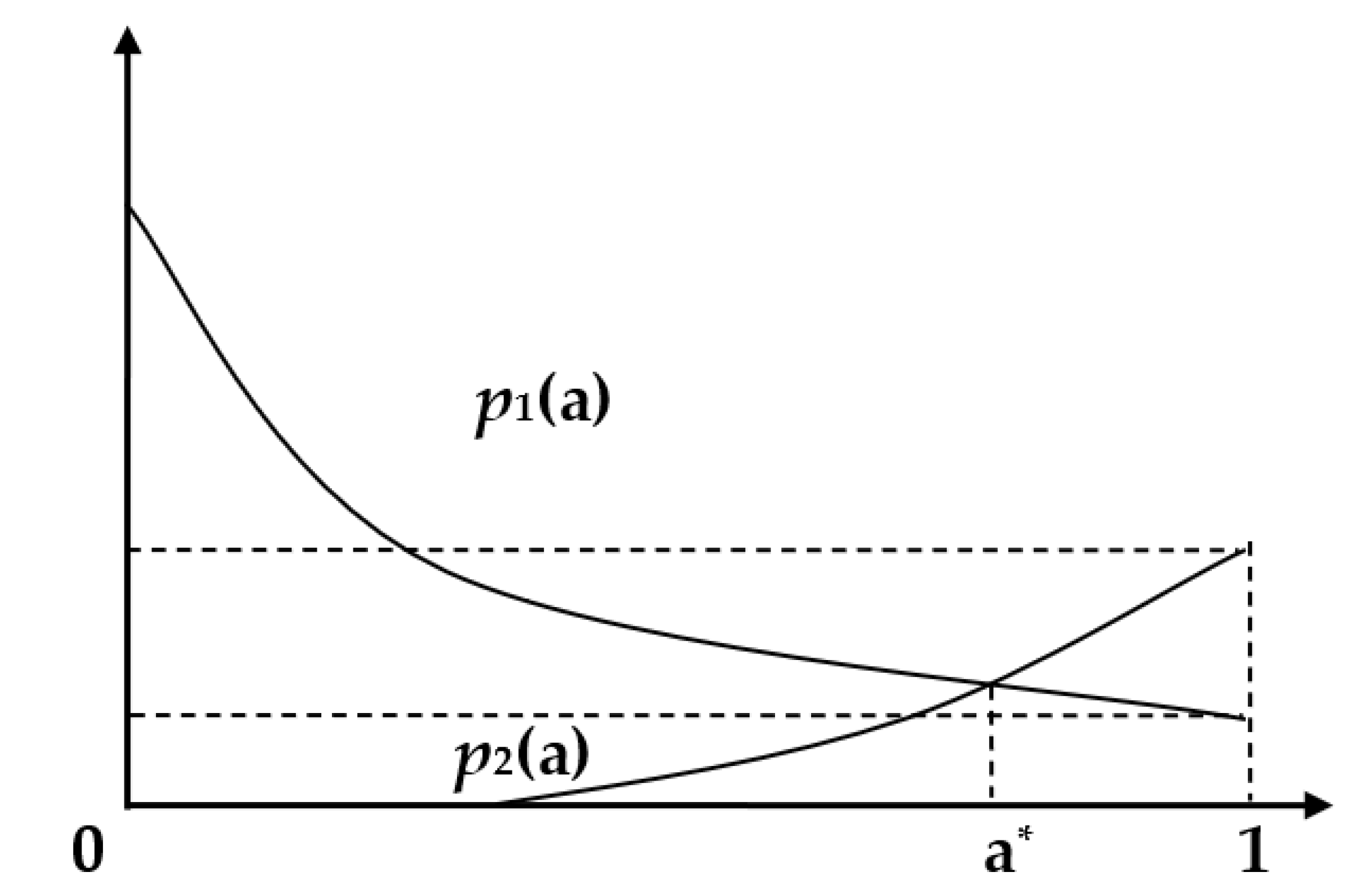
Denote function p 1 ( a ) = d ¯ v β 2 1 a , p 2 ( a ) = 2 d ¯ v β 1 2 + 2 β 2 β 1 2 1 1 a a a 1 a ( 1 a ) , where p 1 ( a ) is monotonically decreasing in 0 < a < 1 and p 2 ( a ) is monotonically increasing on 0 < a < 1 .
It can be seen from Figure 3 that at point a = a where p 1 ( a ) and p 2 ( a ) intersect, there is
min 0 < a < 1 max p 1 ( a ) , p 2 ( a ) = p 2 ( a * ) = p 1 ( a * )
Denote p 3 ( a ) = 2 d ¯ v β 1 2 + 2 β 2 β 1 2 δ a δ , if there is
p 3 ( a ) p 2 ( a ) ,
Then, the minimum error limit is
r 0 = max p 1 ( a ) , p 2 ( a ) , p 3 ( a ) = p 1 ( a ) = d ¯ v / β 2 1 a .
Therefore, the observation error can gradually converge to the region G 0 = { ( x ˜ 1 , x ˜ 2 ) x ˜ 1 r 0 , x ˜ 2 β 1 r 0 } , and the theorem holds. □
Remark 1. 
Compared with the method in [14], the second-order NESO designed according to Theorem 1 has smaller convergence region and higher accuracy, and further considers the stability of observation error in the linear approximation region. At the same time, Theorem 1 gives the design steps for second-order NESO parameter of system: Firstly, the observer gain parameters  β 1 and  β 2 are designed according to the condition (9). Then, the optimal index parameter  a that minimizes the observation error limit can be obtained according to Equation (10). Finally, the parameter  δ in the linear approximation area is obtained according to Equation (11). Obviously,  δ = 2 β 2 / β 1 2 1 1 a meets the requirements. On this basis, the observer parameters have the following relations with the error limit: the larger  β 2 is, the smaller  r 0 is, that is, the error limit of observation error  x ˜ 1 is smaller; the smaller  β 1 is, the smaller  β 1 r 0 is, that is, the error limit of observation error  x ˜ 2 is smaller. Finally, the smaller  a is, the smaller  r 0 is. If the obtained observation error limit does not meet the design requirements, it is only necessary to readjust β 1 and β 2 according to the relationship between the parameters and the error limit, and then obtain the other corresponding parameters according to the above steps.

3. NESO-Assisted Backstepping Variable Structure Attitude Control

In this section, based on the characteristic that the simplified model of HGV-oriented control system design satisfies the generalized matching conditions, the attitude controller is designed using backstepping’s design ideas, combined with variable structure control and NESO.

3.1. Reduced-Order Modeling

At first, we employ the “Reduced-order modeling” idea to transfer the HGV MIMO system into two first-order subsystems. Consider the following forms of MIMO block cascaded nonlinear uncertain system:
x ˙ 1 = a 1 ( x 1 ) + B 1 ( x 1 ) x 2 + d 1 x ˙ 2 = a 2 ( x 1 , x 2 ) + B 2 ( x 1 , x 2 ) x 3 + d 2 x ˙ n = a n ( x 1 , x 2 , , x n ) + B n ( x 1 , x 2 , , x n ) u + d n
where x = x 1 , x 2 , , x n T is the state vector, d 1 , d 2 , , d n is the uncertainty vector, u is the control vector which only appears in the last sub-block, a 1 , a 2 , , a n and B 1 , B 2 , , B n are the known sub-vector fields and sub-control matrices that match the corresponding dimensions, respectively.
Hypothesis 1. 
The sub-control matrix  B 1 ( x 1 ) , B 2 ( x 1 , x 2 ) , , B n ( x 1 , x 2 , , x n ) is uniformly invertible.
A system that satisfies Hypothesis 1 is called a nonlinear system that satisfies the generalized matching condition. In system (31), d n is the matching uncertainty and d 1 , d 2 , , d n 1 are all non-matching uncertainties.
If the system can be written in the strict feedback form of Formula (31), then the idea of backstepping can be used to design the stability control law. The backstepping method decomposes the design problem of the whole system into a series of low-order subsystem design problems. For the cascaded low-order subsystem system, the compound Lyapunov function is used step by step from outside to inside to obtain the feedback control that stabilizes the whole system.
Classify the nonlinear dynamics of a large-scale changes in the system as aggregate uncertainties and denote n = 2 , then
x 1 = Ω , x 2 = ω , a 1 x 1 = 0 , B 1 x 1 = N Ω , d 1 = f 1 Ω a 2 x 1 , x 2 = 0 , B 2 x 1 , x 2 = B ¯ Ω = J ¯ 1 C ¯ δ Ω , d 2 = f 2 Ω , ω + B Ω B ¯ Ω u
where C ¯ δ ( Ω ) is the nominal value of the aerodynamic moment parameter matrix and J ¯ = d i a g { J ¯ x 1 , J ¯ y 1 , J ¯ z 1 } is the nominal value of the moment of inertia matrix.
The model (39) in [6] for control system design can be written in the form of Equation (31):
x ˙ 1 = a 1 x 1 + B 1 x 1 x 2 + d 1 x ˙ 2 = a 2 x 1 , x 2 + B 2 x 1 , x 2 u + d 2
Since the BTT strategy is adopted for flight and the side slip angle β 90 during the whole flight, the sub-control matrix B 1 ( x 1 ) is reversible and the sub-control matrix B 2 ( x 1 , x 2 ) is also uniformly reversible. Therefore, the model for control system design is an uncertain nonlinear system satisfying the generalized matching condition, in which d 1 is the non-matching uncertainty and d 2 is the matching uncertainty.

3.2. Improved Backstepping Control

Traditional backstepping method needs to obtain the derivative information of the pseudo-control in each intermediate step, and the acquisition of these derivatives often requires complicated analytical operations. Aiming at this problem, this section proposes an improved backstepping control method. By introducing the pseudo-control filter and the correcting the error signal, the derivative of the pseudo-control can be easily obtained, and the design is simplified.
For the following nonlinear nominal systems:
x ˙ 1 = a 1 x 1 + B 1 x 1 x 2 x ˙ 2 = a 2 x 1 , x 2 + B 2 x 1 , x 2 u 0
Define the tracking error e 1 = x 1 x 1 r and K1, K2 are the control gain. First, the ideal pseudo control amount x 2 = x 2 c is designed so that e 1 can gradually converge to the origin.
Then, define the Lyapunov function V 1 = 1 2 e 1 T e 1 , and we have
V ˙ 1 = e 1 T e ˙ 1 = e 1 T a 1 + B 1 x 2 c x ˙ 1 r
Obviously, taking
x 2 c = B 1 1 K 1 e 1 a 1 + x ˙ 1 r , K 1 > 0
we get V ˙ 1 = e 1 T K 1 e 1 < 0 , e 1 0 .
Next, in order to avoid the complicated analytical solution of x ˙ 2 c in the next control solution, the following pseudo-control filter bank is introduced to filter each component of x 2 c , which simplifies the design of the backstepping controller.
q ˙ 1 i = q 2 i q ˙ 2 i = 2 ς f i ω f i [ S R i ( ω f i 2 2 ς ω f i [ S M i ( x 2 c i ) q 1 i ] ) q 2 i ]
x 2 r x ˙ 2 r = q 1 q 2
Here, x 2 r is substituted for x 2 c as the intermediate pseudo control variable. Among them, ς f i is the damping ratio, which can usually be set to 1. ω f i is the frequency of the filter, which should be large so that the pseudo control variable can quickly approach the ideal pseudo control variable x 2 c , and the influence of removing high frequency noise should be considered too. S M i and S R i are amplitude saturation function and rate saturation function, respectively, whose saturation value is determined according to the limit allowable values of each state x 2 i and x ˙ 2 i . It can be seen that by using the pseudo control filter to get the intermediate pseudo control variable x 2 r , the constraints on the actual limit of the bandwidth and the amplitude and rate of the system state can be considered, and the derivative x ˙ 2 r of the pseudo control variable can be easily obtained. Therefore, the solution of the subsequent control variable is greatly simplified.
Since the pseudo control variable used is x 2 r instead of ideal x 2 c , the influence of this substitution should be considered. The tracking error is corrected to eliminate the error caused by substitution. Therefore, a new variable γ 1 is introduced to measure the influence of substitution.
γ ˙ 1 = K 1 γ 1 + B 1 x 2 r x 2 c
Subtract the influence from the tracking error, and the tracking error e 1 is corrected to e ¯ 1 = e 1 γ 1 = x 1 x 1 r γ 1 .
Define the tracking error e 2 = x 2 x 2 r and construct a composite Lyapunov function V 2 = 1 2 e ¯ 1 T e ¯ 1 + 1 2 e 2 T e 2 , meanwhile differentiate V 2 :
V ˙ 2 = e ¯ 1 T x ˙ 1 x ˙ 1 r g ˙ 1 + e 2 T x ˙ 2 x ˙ 2 r
Substituting Equations (33) and (38) into Equation (39), we get:
V ˙ 2 = e ¯ 1 T a 1 + B 1 e 2 + x 2 r x ˙ 1 r + K 1 γ 1 B 1 x 2 r x 2 c + e 2 T x ˙ 2 x ˙ 2 r = e ¯ 1 T a 1 + B 1 e 2 x ˙ 1 r + K 1 γ 1 + B 1 x 2 c + e 2 T x ˙ 2 x ˙ 2 r
Substituting Equation (35) into Equation (40), we get:
V ˙ 2 = e ¯ 1 T B 1 e 2 + K 1 γ 1 K 1 e 1 + e 2 T x ˙ 2 x ˙ 2 r = e ¯ 1 T K 1 e ¯ 1 + e ¯ 1 T B 1 e 2 + e 2 T a 2 + B 2 u 0 x ˙ 2 r
Obviously,
u 0 = B 2 1 B 1 T e ¯ 1 a 2 + x ˙ 2 r K 2 e 2 , K 2 > 0
Then
V ˙ 2 = e ¯ 1 T K 1 e ¯ 1 e 2 T K 2 e 2 < 0
Therefore, the use of an improved backstepping controller u 0 for the nominal system can make the tracking errors e ¯ 1 and e 2 converge to the origin gradually.

3.3. NESO-Assisted Backstepping Variable Structure Attitude Controller Design

For the HGV model converted into the strict feedback form (32), due to the large-scale change of aircraft parameters, the aggregated uncertainties d 1 , d 2 will also change widely. If backstepping controller is used for the nominal nonlinear system, a large control gain K 1 , K 2 must be taken to ensure the tracking accuracy of the system. However, this can easily cause the saturation of the control variables, which will result in the instability of the closed-loop system. If more accurate estimates of d 1 , d 2 can be obtained in real time, they can be compensated correctly according to the estimates of uncertainty. In this case, only a small control gain is needed to achieve the required tracking accuracy.
The following two sets of NESO are designed to estimate the non-matching uncertainty d 1 and the matching uncertainty d 2 , respectively:
x ˜ 1 = z 1 x 1 = x ˜ 11 x ˜ 12 x ˜ 13 T z ˙ 1 = N x 2 + z 2 b 1 x ˜ 1 z ˙ 2 = b 2 f a l x ˜ 1 , a 1 , d 1
x ˜ 2 = z 3 x 2 = x ˜ 21 x ˜ 22 x ˜ 23 T z ˙ 3 = B ¯ u + z 4 β 3 x ˜ 2 z ˙ 4 = β 4 f a l x ˜ 2 , a 2 , δ 2
d ^ 1 = z 2
d ^ 2 = z 4
Among them, the first group of NESO includes three second-order NESOs with the same parameters. z 1 = z 11 z 12 z 13 T is the estimated value of the flight attitude x 1 = γ V β α T , and z 2 is the estimated value of the non-matching uncertainty d 1 ; the second group of NESO also includes three second-order NESOs with the same parameters. z 3 = z 31 z 32 z 33 T is the estimated value of the airframe axial angular velocity x 2 = [ ω x 1 ω y 1 ω z 1 ] T , and z 4 is the estimated value of the matching uncertainty d 2 .
The estimate of the uncertainty is essentially the integration of the nonlinear function of the state estimation error of the original system. In order to avoid the NESO’s peak phenomenon and the transient process of the observer’s convergence, which would damage the stability of the system, the estimated signal of NESO is introduced only when NESO is stable, and the estimation is more accurate.
In order to further adapt to the changing nonlinear dynamics and improve the disturbance rejection performance of the whole closed-loop system, a backstepping variable structure attitude controller based on NESO is proposed in this section. The basic principle is as follows: When NESO is in a transient state and the estimation is not accurate, an improved backstepping controller with a larger control gain is used. When the NESO estimation is accurate and stable, the NESO estimation signal is added, and the ability of NESO to capture the unknown dynamic and uncertainty quickly is used to correct the control signal in time and reduce the control gain.
The backstepping variable structure attitude controller based on NESO is designed as follows:
x 2 c = N 1 K 1 e 1 + x ˙ 1 r d ^ 1
u = B ¯ 1 N T e ¯ 1 + x ˙ 2 r K 2 e 2 d ^ 2
Among them, the control matrix K 1 = d i a g { k 11 , k 12 , k 13 } , K 2 = d i a g { k 21 , k 22 , k 23 } and the NESO control signal d ^ 1 = d ^ 11 d ^ 12 d ^ 13 T , d ^ 2 = d ^ 21 d ^ 22 d ^ 23 T . In the control law, taking different values according to the quality of uncertainty estimation is also a kind of variable structure control essentially.
Here, the method of sliding window test to estimate the peak value of the error is used to monitor the quality of the uncertainty estimate by NESO. First, the observation errors of the most recent period are stored, and the peak value of the observation errors in this period is extracted. Then, the observed error peak is compared with a set threshold. If the peak value of the observation error within this time period is less than the threshold, it indicates that NESO has stabilized and converged, and the estimation of uncertainty is more accurate. Finally, the estimated signal of NESO can be added to the control.
The design sliding window length is N . x ˜ i j ( N ) is the vector which is composed of the absolute value of the observation error of a state at the previous N times (including the present time), T h i j , e s t is the estimation accuracy threshold of NESO in this state, and d ^ i j is the uncertainty estimation signal output by NESO to the control.
x ˜ i j , max = max { x ˜ i j ( N ) } ; i = 1 , 2 ; j = 1 , 2 , 3
k i j = k ¯ i j x ˜ i j , max < T h i j , e s t k _ i j , x ˜ i j , max T h i j , e s t
d ^ i j = z ( i + 1 ) j x ˜ i j , max < T h i j , e s t 0 , x ˜ i j , max T h i j , e s t
Next, the stability of the closed-loop system after the augmentation of the expanded state observer is discussed.
The derivative of the composite Lyapunov function V 2 = 1 2 e ¯ 1 T e ¯ 1 + 1 2 e 2 T e 2 is
V ˙ 2 = e ¯ 1 T K 1 e ¯ 1 + e ¯ 1 T N e 2 + e ¯ 1 T d 1 d ^ 1 + e 2 T B ¯ u + d 2 x ˙ 2 r = e ¯ 1 T K 1 e ¯ 1 + e ¯ 1 T d ˜ 1 e 2 T K 2 e 2 + e 2 T d ˜ 2
It can be seen from the above formula that the uncertainty estimation error d ˜ 1 = d 1 d ^ 1 , d ˜ 2 = d 2 d ^ 2 has a great influence on the stability of the closed-loop system. As shown in Theorem 1, if the uncertainty’s change rate does not exceed the assumed value, the parameters of the extended state observer are properly designed, and the estimation speed is fast enough, then after a short time, the estimation error d ˜ 1 , d ˜ 2 can converge to a small stable sate value d ˜ 1 * , d ˜ 2 * . Therefore, by selecting appropriate K 1 , K 2 , it can be satisfied that V ˙ 2 is negatively definite outside a sufficiently small area Ω = e ¯ 1 , e 2 | e ¯ 1 i d ˜ 1 i * / k _ 1 i , e 2 i d ˜ 2 i * / k _ 2 i of the origin e ¯ 1 = 0 , e 2 = 0 after a finite time. This also proves that the tracking error e ¯ 1 , e 2 is uniformly ultimately bounded. Due to the short adjustment time of the pseudo control filter, the pseudo control x 2 r can quickly approach the ideal value x 2 c , and γ 1 will also quickly converge to 0. Therefore, after a finite time, the attitude angle tracking error will converge to the following areas:
Ω = e 1 | e 1 i d ˜ 1 i * / 2 k _ 1 i r * , r * = d ˜ 1 i * 2 / 4 k _ 1 i 2 + d ˜ 2 i * 2 / k _ 1 i k _ 2 i
The backstepping attitude controller based on NESO has the following characteristics:
(1)
The attitude control is realized by angular velocity tracking pseudo control, and the tracking of the angle velocity to the pseudo control is realized by the control torque generated from the pneumatic rudder surface. Based on the idea of backstepping, the influence of the inner loop angle velocity tracking error on the outer loop attitude tracking error is eliminated without the separation of the inner and outer loop time scale.
(2)
In order to solve the problem that the analytical expression of the pseudo control derivative in the traditional backstepping control is difficult to calculate, the pseudo control filter is used to simplify the solution of the pseudo control derivative and the influence of the introduction of the pseudo control filter on the tracking error is eliminated by modifying the tracking error signal. At the same time, the limitation on the state of the system and the influence of reducing noise can also be considered in the design of the pseudo control filter.
(3)
In order to overcome the shortcomings of poor robustness and easy to saturate control quantity of simple backstepping control, NESO is introduced to augment backstepping controller. Once the derivative of uncertainty is bounded, the design of appropriate observer parameters can make the estimation error quickly converge, and the control torque can change accordingly with the actual change of uncertainty, which improves the robustness to uncertainty under the premise of economical control.
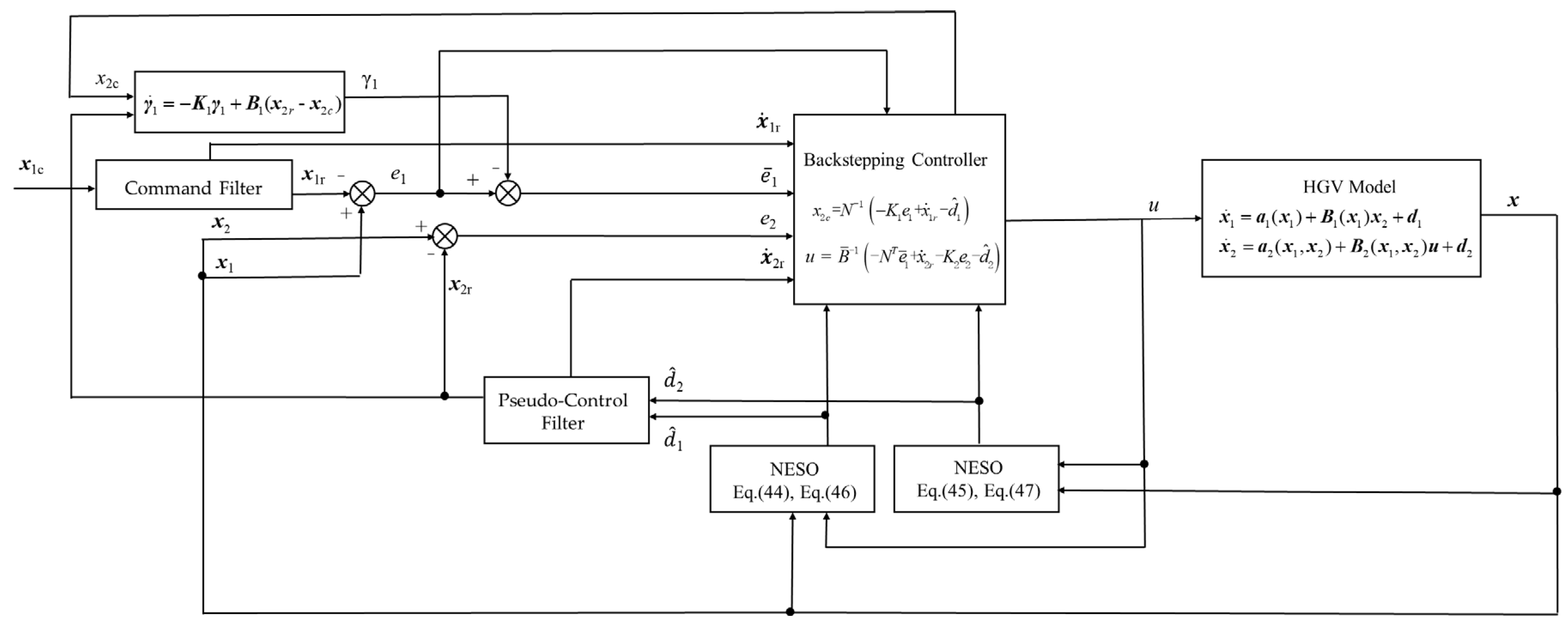
The input of the whole system is denoted as x 1 c , the instruction signal x 1 c will be sent to the command filter, and the signal will be smoothed to be derivable as x 1 r . Then, the general diagram of HGV attitude control system is shown in Figure 4 as follows:

4. Simulations and Results

The parameters of attitude controller are selected as follows:
Command filter: r α = 20 / s 2 , r γ V = 5 / s 2 ;
Control gain: k _ 11 = k _ 12 = k _ 13 = 1 , k ¯ 11 = k ¯ 12 = k ¯ 13 = 1.5 ;
k _ 21 = k _ 22 = k _ 23 = 1 , k ¯ 21 = k ¯ 22 = k ¯ 23 = 5 ;
Pseudo control filter:
damping ratio ς f i = 1 ; natural frequency ω f i = 5 ;
rate limits S R 1 = ± 0.5 rad / s 2 , S R 2 = ± 0.5 rad / s 2 , S R 3 = ± 2 rad / s 2 ;
amplitude limits S M 1 = ± 0.3 rad / s , S M 1 = ± 0.1 rad / s , S M 1 = ± 0.5 rad / s ;
NESO parameters: β 1 = 30 ; β 2 = 50 ; a 1 = 0.75 ; δ 1 = 1.5 × 10 4 ;
β 3 = 100 ; β 4 = 500 ; a 2 = 0.65 ; δ 2 = 0.015 ;
Variable structure thresholds: T h 1 j , e s t = 0.001 , T h 2 j , e s t = 0.005 , j = 1 , 2 , 3 .
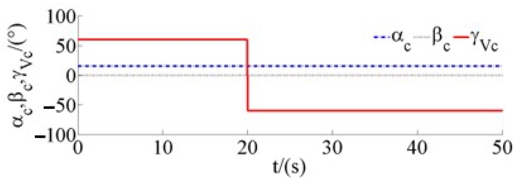
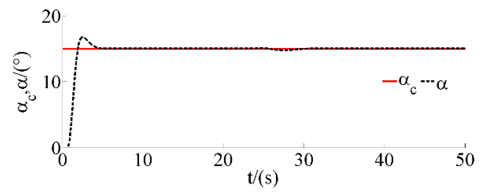
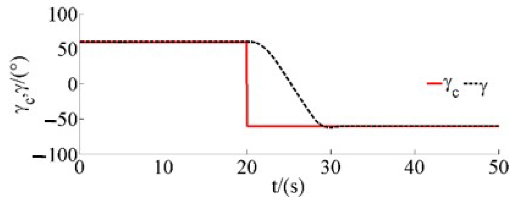
The given step attitude command is shown in Figure 5 and the smooth reference attitude filtered by the command filter is shown in Figure 6. The angle of attack reference command reaches 15° in 2 s, and the roll angle reference command completes the sign inversion from 60° to −60° in 10 s.
Constant external disturbance M d x = 50   N m , M d y = 10   N m , M d z = 100   N m are added to the simulation. First, the states in Table 2 are used as initial conditions for simulation.
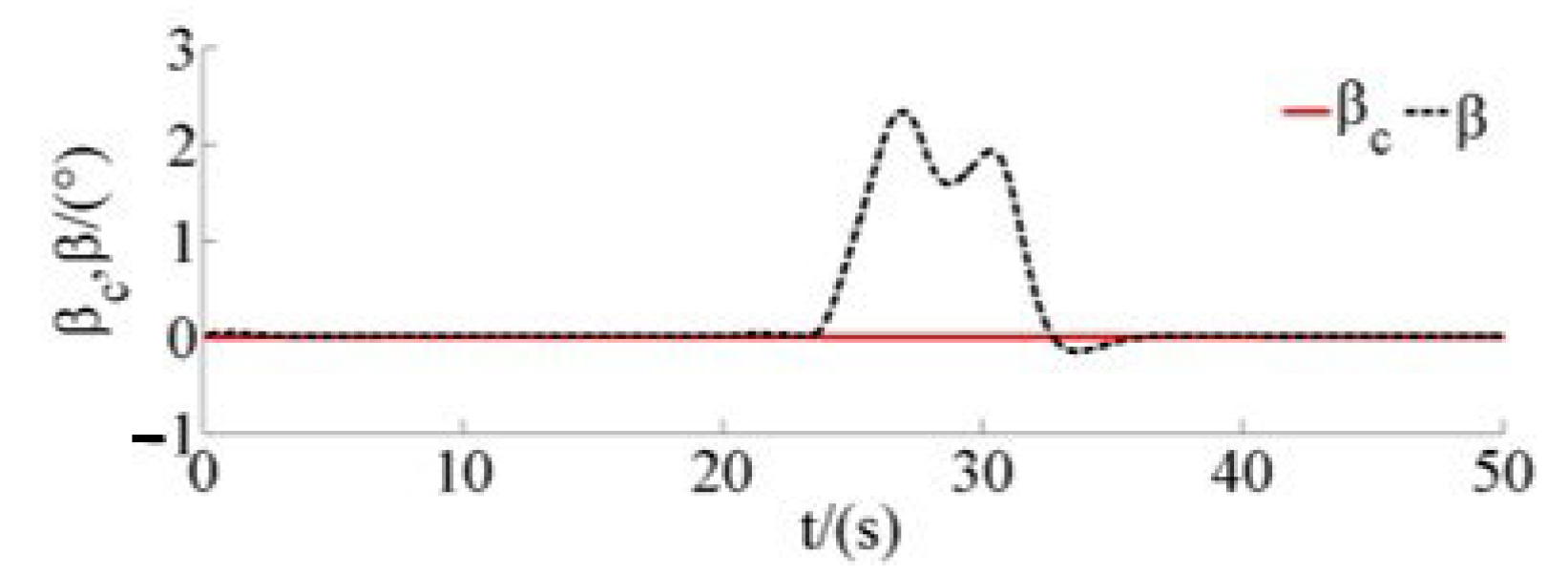
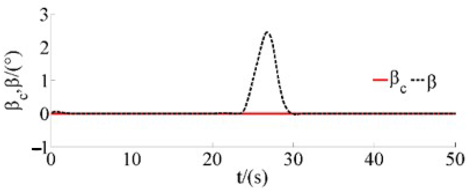
The attitude angle tracking error (the difference between the actual attitude and the reference attitude) is shown in Figure 7, and the steady-state tracking error is less than 0.05°. As can be seen in Figure 8, the rise time of the angle of attack tracking is 1.4 s, the adjustment time is 4 s, and the overshoot is 0.148° less than 1%. Figure 9 shows that during the inversion of the bank angle, the sideslip angle will deviate due to the influence of the coupling and the deviation peak is 2.33°, which is within the given allowable deviation range. At the same time, it can be seen from Figure 10 that the rise time of the bank angle tracking is 7.5 s, the adjustment time is 8.47 s, and the overshoot is 2.6 ° less than 2.2%.
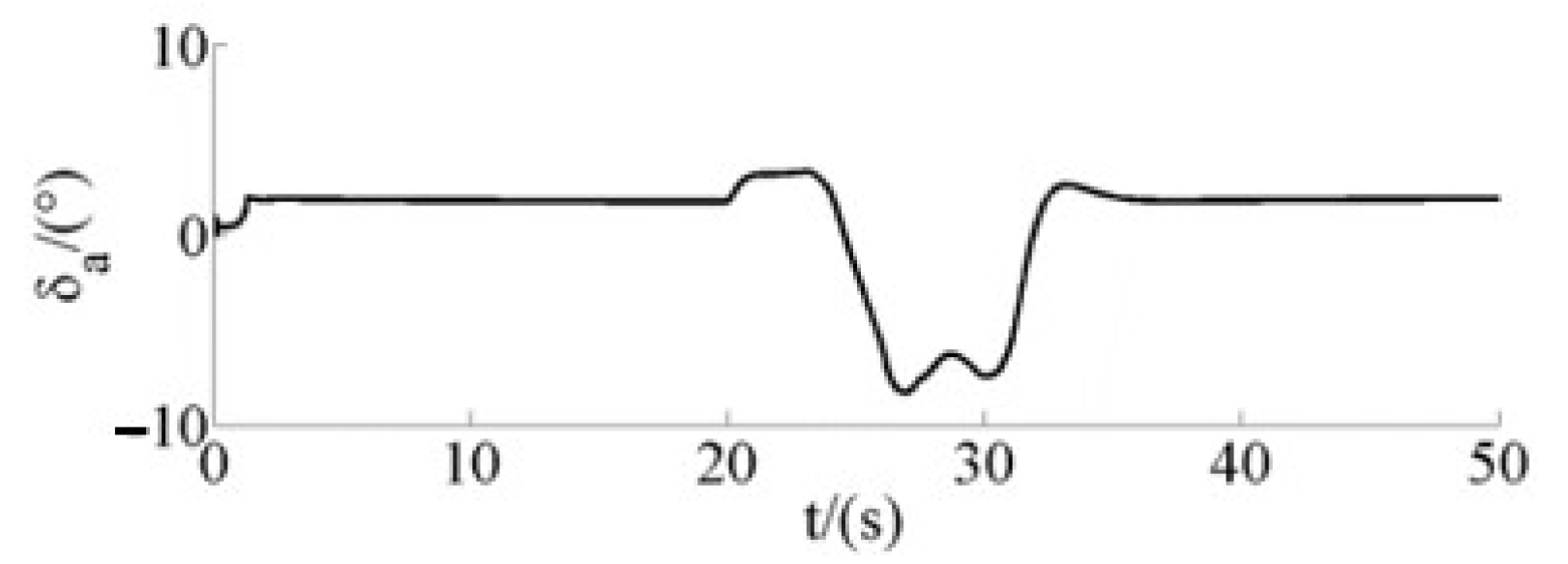
The historical deflections of each aerodynamic rudder surface are shown in Figure 11, Figure 12 and Figure 13. The deflections of each rudder surface are within the limit of amplitude, the control signal is smooth, and only the rudder appears to be saturated for a short time in the process of the reverse signal of bank angle. In order to offset the constant disturbance torque, each rudder surface keeps a certain rudder deviation during steady state.
The intermediate pseudo control signals of backstepping are shown in Figure 14 and Figure 15.
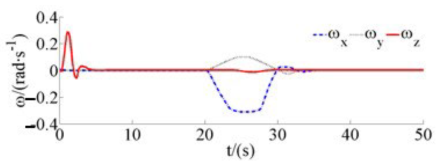
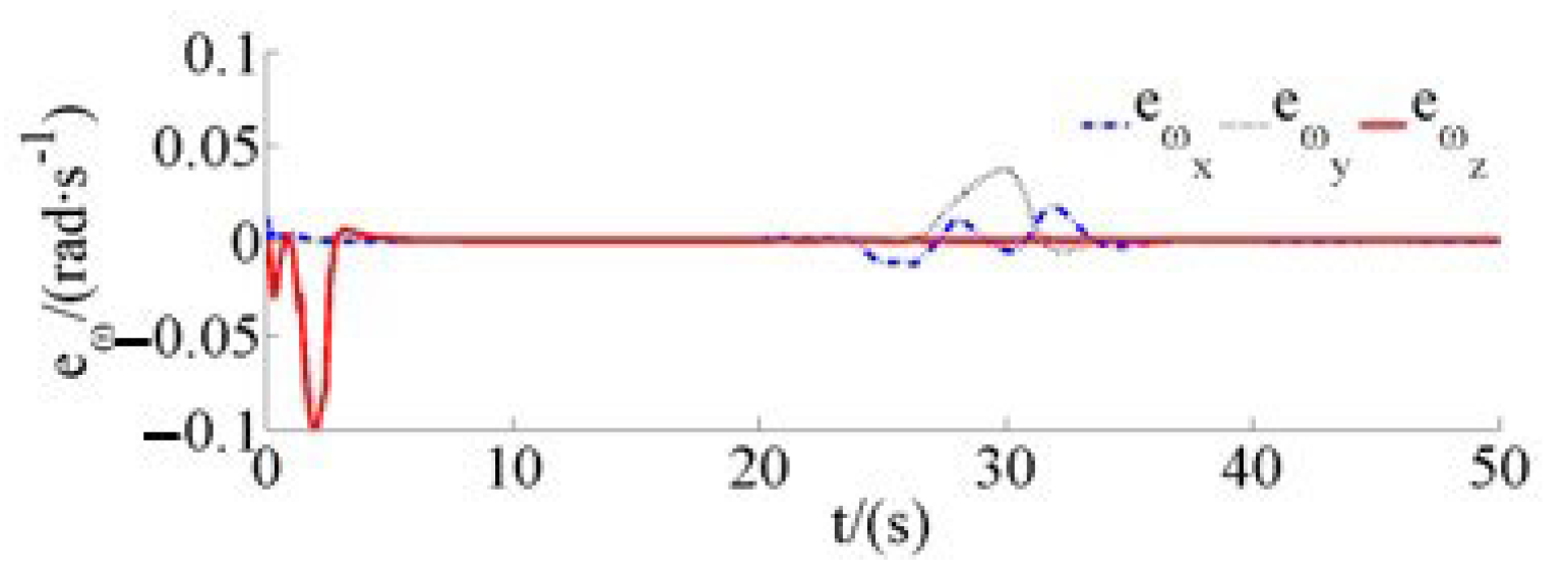
Figure 14 is the ideal pseudo control signal, and Figure 15 is the actual pseudo-control signal obtained after smoothing and limiting by the pseudo control filter. Figure 16 shows the rotation angular velocity of the aircraft around the airframe axis. During the flight, the maximum pitch angular velocity is 0.29 rad/s, the maximum roll angular velocity is −0.31 rad/s, and the maximum yaw angular velocity is 0.1 rad/, which basically meets the amplitude limit designed in advance for the pseudo control filter. Figure 17 shows the tracking of the body angular velocity to the pseudo control command, and the fast tracking of the angular velocity to the pseudo control ensures the convergence of the attitude error.
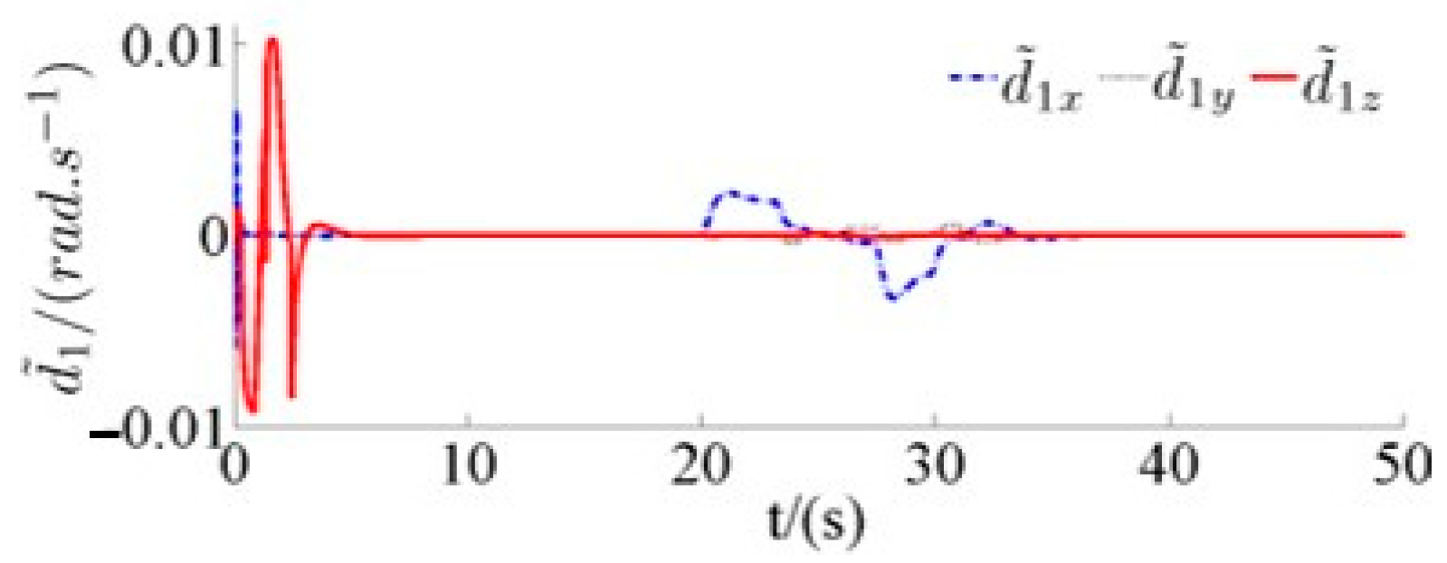
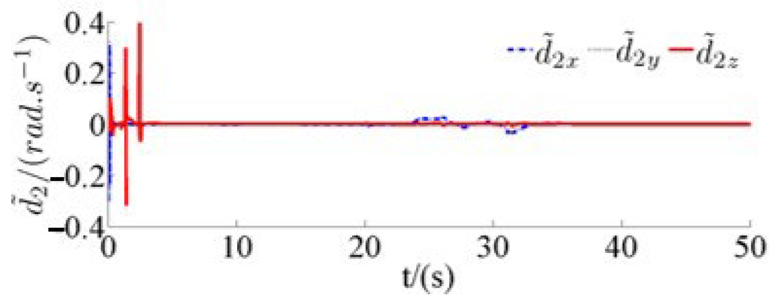
Figure 18 and Figure 19 show the estimation effect of two groups of NESO on matching uncertainty and non-matched uncertainty, respectively. It can be seen from the figure that when the uncertainty changes greatly, there is a large estimation error, and when the uncertainty changes little, the estimated signal is stable and accurate.
At the same time, the simulation of simple backstepping controller without NESO is also carried out in this section. The simulation results are shown in Figure 20, Figure 21 and Figure 22. Due to the poor robust performance of the backstepping controller, the tracking of body angular velocity and attitude tends to oscillate and diverge obviously in the presence of uncertainty.
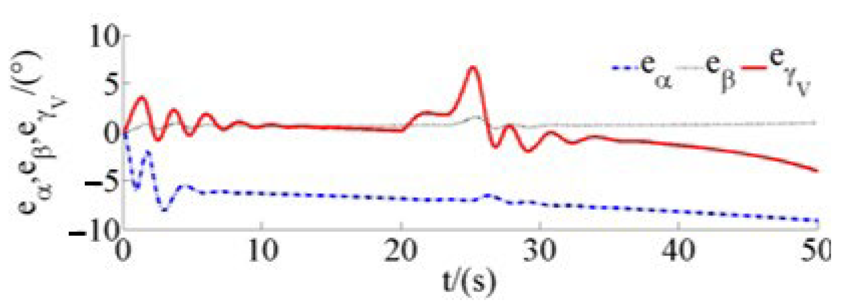
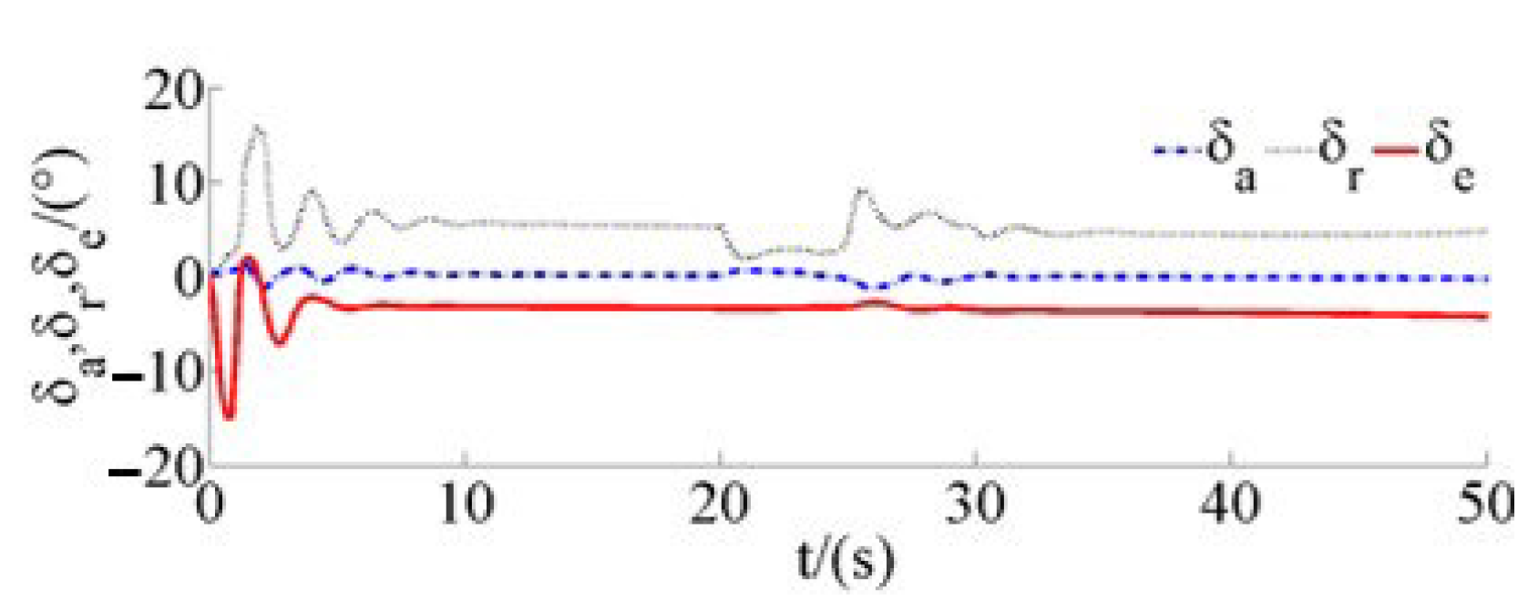
In order to illustrate the adaptability of the backstepping variable structure attitude controller based on NESO to the wide range changes of aircraft parameters, the initial conditions of simulation in Table 1 are changed to height 35 km and speed 2600 m/s, and the same attitude controller is used for simulation. From Figure 23, Figure 24, Figure 25 and Figure 26, it can be seen that although the parameters of the aircraft have changed greatly with the change of initial conditions, the controller can still achieve stable and accurate flight attitude tracking.

5. Conclusions

Aiming at solving the control problem caused by the large-scale change of vehicle parameters, this paper proposes a design method of backstepping variable structure attitude controller based on NESO, with the characteristics of HGV model and the idea of uncertainty estimation and compensation associated.
Firstly, the structure of the ESO is introduced, and the design of the second-order NESO is studied in detail. Due to the large number of NESO parameters, a systematic method for determining the second-order NESO parameters is given in this paper. And the stability of the observer is proved completely using the piecewise Lyapunov analysis.
Then, based on the idea of backstepping, the backstepping variable structure attitude controller based on NESO decomposes the whole system design problem into two first-order subsystem design problem and classifies the nonlinear dynamic changes caused by the large-scale changes of the vehicle parameters into the aggregated uncertain terms of the two subsystems. Firstly, an improved backstepping controller is designed for the nominal system. The traditional backstepping method is improved by introducing command filtering and error signal correction, which simplifies the solution of the derivative of the pseudo control variable and ensures the stability of the nominal system. Then, combining NESO with improved backstepping control, a backstepping variable structure attitude controller based on NESO is designed. Using two sets of NESOs to estimate the matching and non-matching uncertainties, respectively, the working condition of each NESO is monitored by using a sliding window test to estimate the peak value of the error. According to the quality of NESO’s uncertainty estimation, it switches between backstepping control and NESO-based backstepping control, which solves the problem of large gain of backstepping control and improves the disturbance rejection performance of the controller. The simulation results show that the backstepping attitude controller based on NESO can realize the stable and accurate tracking of the flight attitude when the aircraft parameters change in a large range.
Finally, the control accuracy of the attitude controller based on the NESO studied in this paper is closely associated with the convergence speed and accuracy of the ESO, and the latter is greatly affected by the uncertainty’s change rate. Therefore, this method is only suitable for situations where the parameters of the vehicle do not change too quickly. For drastic changes in HGV parameters and external disturbances, new theories and methods are required to further explore the design of the attitude controller. In future research, we will study the design of intelligent, adaptive, and antidisturbance controllers [41,42,43,44,45] for control problems of drastic dynamic changes of HGV parameters and external disturbances.

Author Contributions

Conceptualization, J.C.; methodology, W.L. and J.C.; software, W.L. and J.C.; validation, W.L., H.L., R.Z. and J.C.; formal analysis, W.L., H.L. and J.C.; investigation, W.L., H.L. and J.C.; resources, J.C.; data curation, W.L., H.L. and R.Z.; writing—original draft preparation, W.L. and J.C.; writing—review and editing, J.C.; visualization, W.L.; supervision, J.C.; project administration, J.C.; funding acquisition, J.C. All authors have read and agreed to the published version of the manuscript.

Funding

This work was supported in part by the National Key Research and Development Program of China under Grant 2022YFD2001405; in part by the Open Project Program of Key Laboratory of Smart Agricultural Technology in Tropical South China, Ministry of Agriculture and Rural Affairs, under Grant HNZHNY-KFKT-202202; in part by the Open Fund of Key Laboratory of Urban Land Resources Monitoring and Simulation, Ministry of Natural Resources, under Grant KF-2021-06-115; in part by the Key Laboratory of Spatial-temporal Big Data Analysis and Application of Natural Resources in Megacities, MNR, under Grant KFKT-2022-05; in part by the National Natural Science Foundation of China under Grant 51979275; in part by the Earmarked Fund for CARS-20; in part by the Open Project Program of State Key Laboratory of Virtual Reality Technology and Systems, Beihang University, under Grant VRLAB2022C10; in part by the Jiangsu Province and Education Ministry Co-sponsored Synergistic Innovation Center of Modern Agricultural Equipment under Grant XTCX2002; in part by the 2115 Talent Development Program of China Agricultural University; and in part by the Chinese Universities Scientific Fund under Grant 2021TC105.

Data Availability Statement

Some data, models, or code generated or used during the study are available from the corresponding author by request.

Conflicts of Interest

The authors declare no conflict of interest.

References

  1. An, K.; Guo, Z.-Y.; Xu, X.-P.; Huang, W. A Framework of Trajectory Design and Optimization for the Hypersonic Gliding Vehicle. Aerosp. Sci. Technol. 2020, 106, 106–110. [Google Scholar] [CrossRef]
  2. Hutchinson, R.; Lawrence, J.; Joiner, K.F. Conceptual design and integration of a propulsion system for a supersonic transport aircraft. Proc. Inst. Mech. Eng. Part G J. Aerosp. Eng. 2022, 236, 583–592. [Google Scholar] [CrossRef]
  3. Le, V.T.; San Ha, N.; Goo, N.S. Advanced sandwich structures for thermal protection systems in hypersonic vehicles: A review. Compos. Part B Eng. 2021, 226, 109301. [Google Scholar] [CrossRef]
  4. Bai, C.; Chen, J.; Ren, Z.; Li, Q.; Xiong, Z. Adaptive decoupling control of hypersonic vehicle using fuzzy-neural network observer. Proc. Inst. Mech. Eng. 2016, 230, 1216–1223. [Google Scholar] [CrossRef]
  5. Chen, J.; Zhao, Q.; Liang, Z.; Li, P.; Ren, Z.; Zheng, Y. Fractional calculus guidance algorithm in a hypersonic pursuit-evasion game. Def. Sci. J. 2017, 67, 688–697. [Google Scholar] [CrossRef]
  6. Chen, J.; Du, N.; Han, Y. Decoupling attitude control of a hypersonic glide vehicle based on a nonlinear extended state observer. Int. J. Aerosp. Eng. 2020, 2020, 1–11. [Google Scholar] [CrossRef]
  7. Gao, Z.; Huang, Y.; Han, J. An alternative paradigm for control system design. In Proceedings of the IEEE Conference on Decision and Control, Orlando, FL, USA, 4–7 December 2001; pp. 4578–4585. [Google Scholar]
  8. Zheng, Q.; Gao, L.Q.; Gao, Z. On stability analysis of active disturbance rejection control for nonlinear time-varying plants with unknown dynamics. In Proceedings of the IEEE Conference on Decision and Control, New Orleans, LA, USA, 12–14 December 2007; pp. 3501–3506. [Google Scholar]
  9. Yoo, D.; Yau, S.T.; Gao, Z. On convergence of the linear extended state observer. In Proceedings of the IEEE International Conference on Control Applications, Munich, Germany, 4–6 October 2006; IEEE: Piscataway, NJ, USA, 2006. [Google Scholar]
  10. Han, J. From PID to active disturbance rejection control. IEEE Trans. Ind. Electron. 2009, 56, 900–906. [Google Scholar] [CrossRef]
  11. Huang, Y.; Han, J. A new synthesis method for uncertain systems the Self-Stable Region approach. Asian Control. Conf. 1999, 30, 33–38. [Google Scholar] [CrossRef]
  12. Huang, Y.; Han, J. Analysis and design for the second order nonlinear continuous extended states observer. Chin. Sci. Bull. 2000, 45, 1938–1944. [Google Scholar] [CrossRef]
  13. Huang, Y.; Xu, K.; Han, J.; Lam, L. Flight control design using extended state observer and non-smooth feedback. In Proceedings of the IEEE Conference on Decision and Control, Orlando, FL, USA, 4–7 December 2001; pp. 223–228. [Google Scholar]
  14. Zhang, R.; Han, J. Parameter identification by model compensation auto disturbance rejection controller. Control Theory Appl. 2000, 17, 79–81. [Google Scholar]
  15. Pu, Z.; Yuan, R.; Yi, J.; Tan, X. A class of adaptive extended state observers for nonlinear disturbed systems. IEEE Trans. Ind. Electron. 2015, 62, 5858–5869. [Google Scholar] [CrossRef]
  16. Utkin, V. Variable structure systems with sliding modes. IEEE Trans. Autom. Control 1977, 22, 212–222. [Google Scholar] [CrossRef]
  17. Young, K.D.; Utkin, V.I.; Ozguner, U. A control engineer’s guide to sliding mode control. IEEE Trans. Control Syst. Technol. 1999, 7, 328–342. [Google Scholar] [CrossRef]
  18. Song, S.; Zhang, B.; Xia, J.; Zhang, Z. Adaptive Backstepping Hybrid Fuzzy Sliding Mode Control for Uncertain Fractional-Order Nonlinear Systems Based on Finite-Time Scheme. IEEE Trans. Syst. Man Cybern.: Syst. 2020, 50, 1559–1569. [Google Scholar] [CrossRef]
  19. Hao, L.Y.; Zhang, H.; Yue, W.; Li, H. Fault-tolerant Compensation Control Based on Sliding Mode Technique of Unmanned Marine Vehicles Subject to Unknown Persistent Ocean Disturbances. Int. J. Control. Autom. Syst. 2020, 18, 739–752. [Google Scholar] [CrossRef]
  20. Xu, C.; Tong, D.; Chen, Q.; Zhou, W.; Shi, P. Exponential stability of Markovian jumping systems via adaptive sliding mode control. IEEE Trans. Syst. Man Cybern. Syst. 2019, 51, 954–964. [Google Scholar] [CrossRef]
  21. Jiang, B.; Karimi, H.R.; Yang, S.; Gao, C.; Kao, Y. Observer-based adaptive sliding mode control for nonlinear stochastic Markov jump systems via T–S fuzzy modeling: Applications to robot arm model. IEEE Trans. Ind. Electron. 2020, 68, 466–477. [Google Scholar] [CrossRef]
  22. Ahmed, S.; Wang, H.; Tian, Y. Adaptive high-order terminal sliding mode control based on time delay estimation for the robotic manipulators with backlash hysteresis. IEEE Trans. Syst. Man Cybern.: Syst. 2019, 51, 1128–1137. [Google Scholar] [CrossRef]
  23. Gao, K.; Li, Q.; Ren, Z.; Bai, C. Observer-based attitude control for hypersonic gliding vehicle. In Proceedings of the 2014 IEEE Chinese Guidance, Navigation and Control Conference, Yantai, China, 8–10 August 2014; IEEE: Piscataway, NJ, USA, 2014; pp. 1159–1162. [Google Scholar]
  24. Liu, X.; Zhang, Y.; Wang, S.; Huang, W. Backstepping attitude control for hypersonic gliding vehicle based on a robust dynamic inversion approach. Proc. Inst. Mech. Eng. Part I J. Syst. Control Eng. 2014, 228, 543–552. [Google Scholar] [CrossRef]
  25. Zhang, P.; Du, Y. The robust maneuver flight control of hypersonic glide vehicles with input saturation using disturbance observer. In Proceedings of the IECON 2017-43rd Annual Conference of the IEEE Industrial Electronics Society, Beijing, China, 29 October–1 November 2017; IEEE: Piscataway, NJ, USA, 2017; pp. 6584–6589. [Google Scholar]
  26. Zhang, Y.; Dong, X.; Yu, J.; Li, Q.; Ren, Z. Robust adaptive control for hypersonic gliding vehicles based on NESO. In Proceedings of the 2017 13th IEEE International Conference on Control & Automation (ICCA), Ohrid, Macedonia, 3–6 July 2017; IEEE: Piscataway, NJ, USA, 2017; pp. 431–436. [Google Scholar]
  27. Zhang, W.; Huang, X.; Gao, X.Z. TS Fuzzy Modelling and Attitude Control for Hypersonic Gliding Vehicles. Math. Probl. Eng. 2017, 2017, 1–14. [Google Scholar]
  28. Chen, E.; Jing, W.; Gao, C.; Zhang, Z. An adaptive control approach for a flexible hypersonic glide vehicle. In Proceedings of the 2018 9th International Conference on Mechanical and Aerospace Engineering (ICMAE), Budapest, Hungary, 10–13 July 2018; IEEE: Piscataway, NJ, USA, 2018; pp. 1–5. [Google Scholar]
  29. Zhao, K.; Cao, D.Q.; Huang, W.H. Maneuver control of the hypersonic gliding vehicle with a scissored pair of control moment gyros. Sci. China Technol. Sci. 2018, 61, 1150–1160. [Google Scholar] [CrossRef]
  30. Wei, P.; Jing, W.; Gao, C. Dynamics and control for hypersonic gliding vehicles equipped with a moving mass and RCS. J. Aerosp. Eng. 2019, 32, 06019003. [Google Scholar] [CrossRef]
  31. Li, P.; Yu, X.; Zhang, Y.; Peng, X. Adaptive multivariable integral TSMC of a hypersonic gliding vehicle with actuator faults and model uncertainties. IEEE/ASME Trans. Mechatron. 2017, 22, 2723–2735. [Google Scholar] [CrossRef]
  32. Yu, X.; Li, P.; Zhang, Y. The design of fixed-time observer and finite-time fault-tolerant control for hypersonic gliding vehicles. IEEE Trans. Ind. Electron. 2017, 65, 4135–4144. [Google Scholar] [CrossRef]
  33. Yu, X.; Li, P.; Zhang, Y. Fixed-time actuator fault accommodation applied to hypersonic gliding vehicles. IEEE Trans. Autom. Sci. Eng. 2020, 18, 1429–1440. [Google Scholar] [CrossRef]
  34. Gu, P.; Qi, R.; Jiang, B. Sliding Mode Tracking Control and GA-based Optimization for Reentry Guidance Subject to Multi-Constraints. In Proceedings of the 2018 IEEE CSAA Guidance, Navigation and Control Conference (CGNCC), Xiamen, China, 10–12 August 2018; IEEE: Piscataway, NJ, USA, 2018; pp. 1–6. [Google Scholar]
  35. Zhai, S.; Yang, J. Piecewise analytic optimized ascent trajectory design and robust adaptive finite-time tracking control for hypersonic boost-glide vehicle. J. Frankl. Inst. 2020, 357, 5485–5501. [Google Scholar] [CrossRef]
  36. An, K.; Guo, Z.-Y.; Huang, W.; Xu, X.-P. Leap trajectory tracking control based on sliding mode theory for hypersonic gliding vehicle. J. Zhejiang Univ.-SCIENCE A 2022, 23, 188–207. [Google Scholar] [CrossRef]
  37. Qian, C.; Sun, C.; Huang, Y.; Mu, C.; Zhang, J.; Zhang, R. Design of flight control system for a hypersonic gliding vehicle based on nonlinear disturbance observer. In Proceedings of the 2013 10th IEEE International Conference on Control and Automation (ICCA), Chongqing, China, 28–30 May 2017; IEEE: Piscataway, NJ, USA, 2013; pp. 1573–1577. [Google Scholar]
  38. Ping, S.; Yanli, D.; Peng, Z.; Kai, X. The nonlinear anti-windup control of hypersonic glide vehicles with input saturation and uncertainties. In Proceedings of the 2017 29th Chinese Control And Decision Conference (CCDC), Hangzhou, China, 12–14 June 2017; IEEE: Piscataway, NJ, USA, 2017; pp. 4631–4637. [Google Scholar]
  39. Liu, X.; Shen, Z. Rapid smooth entry trajectory planning for high lift/drag hypersonic glide vehicles. J. Optim. Theory Appl. 2016, 168, 917–943. [Google Scholar] [CrossRef]
  40. Zhang, Y.; Wang, X.; Tang, S. A globally fixed-time solution of distributed formation control for multiple hypersonic gliding vehicles. Aerosp. Sci. Technol. 2020, 98, 105643. [Google Scholar] [CrossRef]
  41. Wang, S.; Chen, J.; He, X. An adaptive composite disturbance rejection for attitude control of the agricultural quadrotor UAV. ISA Trans. 2022, 129, 564–579. [Google Scholar] [CrossRef]
  42. Zhang, Z.; Wang, S.; Chen, J.; Han, Y. A bionic dynamic path planning algorithm of the micro UAV based on the fusion of deep neural network optimization/filtering and hawk-eye vision. IEEE Trans. Syst. Man Cybern. Syst. 2023, 2023, 1–13. [Google Scholar] [CrossRef]
  43. Zhang, Z.; Chen, J.; Xu, X.; Liu, C.; Han, Y. Hawk-eye-inspired perception algorithm of stereo vision for obtaining orchard 3D point cloud navigation map. CAAI Trans. Intell. Technol. 2022, 2022, 1–15. [Google Scholar] [CrossRef]
  44. Le, W.; Xue, Z.; Chen, J.; Zhang, Z. Coverage path planning based on the optimization strategy of multiple solar powered unmanned aerial vehicles. Drones 2022, 6, 203. [Google Scholar] [CrossRef]
  45. Wang, S.; Han, Y.; Chen, J.; He, X.; Zhang, Z.; Liu, X.; Zhang, K. Weed density extraction based on few-shot learning through UAV remote sensing RGB and multispectral images in ecological irrigation area. Front. Plant Sci. 2022, 12, 3456. [Google Scholar] [CrossRef] [PubMed]
Figure 1. Plane division diagram of observation error.
Drones 07 00119 g001
Figure 2. Schematic diagram of the curve and line positions that meet the conditions.
Drones 07 00119 g002
Figure 3. The optimization of solving parameter a where a is the optimal index parameter which can minimize the observation error limit.
Drones 07 00119 g003
Figure 4. The general diagram of HGV attitude control system.
Drones 07 00119 g004
Figure 5. Step attitude command.
Drones 07 00119 g005
Figure 6. Reference attitude.
Drones 07 00119 g006
Figure 7. Attitude angle tracking error.
Drones 07 00119 g007
Figure 8. Attack angle tracking curve.
Drones 07 00119 g008
Figure 9. Sideslip angle tracking curve.
Drones 07 00119 g009
Figure 10. Bank angle tracking curve.
Drones 07 00119 g010
Figure 11. Aileron deflection.
Drones 07 00119 g011
Figure 12. Rudder deflection.
Drones 07 00119 g012
Figure 13. Elevator deflection.
Drones 07 00119 g013
Figure 14. Ideal pseudo control.
Drones 07 00119 g014
Figure 15. Actual pseudo control.
Drones 07 00119 g015
Figure 16. Body axis angular velocity.
Drones 07 00119 g016
Figure 17. Tracking error of body axis angular velocity.
Drones 07 00119 g017
Figure 18. Estimation error of non-matched uncertainty.
Drones 07 00119 g018
Figure 19. Estimation error of matched uncertainty.
Drones 07 00119 g019
Figure 20. Attitude tracking error of the backstepping controller.
Drones 07 00119 g020
Figure 21. Angular velocity tracking error of the backstepping controller.
Drones 07 00119 g021
Figure 22. Rudder deflection of the backstepping controller.
Drones 07 00119 g022
Figure 23. Attack angle tracking under new initial conditions.
Drones 07 00119 g023
Figure 24. Sideslip angle tracking under new initial conditions.
Drones 07 00119 g024
Figure 25. Bank angle tracking under new initial conditions.
Drones 07 00119 g025
Figure 26. Control rudder deflection under new initial conditions.
Drones 07 00119 g026
Table 1. Different types of control problem and research work on HGV.
Control ProblemSolution MethodEffectAuthor (Year)
Attitude ControlObserver-based approachReduced the static error.Kehan Gao et al. (2014) [23]
Robust dynamic inversion control approachBetter tracking rapidity, accuracy, and stability than traditional dynamic inversion control.Xiaodong Liu et al. (2014) [24]
Modified nonlinear disturbance observerSuccessfully estimated the disturbances and solved input saturation problem.Peng Zhang et al. (2017) [25]
Robust adaptive controller (nominal controller, NESO and compensation controller) Eliminated the nonlinear influence and offset the observation error.Yuan Zhang et al. (2017) [26]
State feedback
fuzzy controller (T-S Fuzzy Modeling)
Better than other local controllers.Weidong Zhang et al. (2017) [27]
Adaptive control approach
based on moving horizon least square method
Effectively controlled the attitude of flexible HGV.Erkang Chen et al. (2018) [28]
Decoupling controller
based on feedback linearization
Significantly increased the airspace range and flexibility of the HGVKun Zhao et al. (2018) [29]
Sliding mode control and adaptive compensation (composed control)High robustness to aerodynamic parameter
Uncertainties.
Pengxin Wei et al. (2019) [30]
Decoupling control method based on a NESOCompensated the channel-coupling to a great extent better than traditional subchannel feedback control.Jian Chen et al. (2020) [6]
Fault-tolerant controlCombined multivariable integral Terminal Sliding Mode Control (TSMC) and adaptive techniquesSolved the actuator gain and bias malfunction in time.Peng Li et al. (2017) [31]
Fixed-time observer and finite-time multivariable TSMCThe estimation error can converge to zero and the fault system can be stably controlled in a limited time.Xiang Yu et al. (2017) [32]
SMC, bilimit homogeneity, and adaptive techniquesEliminiated the tracking error in the case of actuator failure and generated continuous control signals to avoid chattering.Xiang Yu et al. (2020) [33]
Trajectory tracking controlSliding mode tracking controlImproved the ability of robustness of the reentry gliding of HGVPanfei Gu et al. (2018) [34]
Robust adaptive controllerThe tracking error converges to a small neighborhood close to zero in finite time.Sheng Zhai et al. (2020) [35]
A combined super-twisting sliding mode
Controller
Had strong robustness to initial uncertain parameters and other disturbances and appropriate gain.Kai An et al. (2022) [36]
Disturbance rejection controlNonlinear disturbance observer and sliding mode controllerEstimated unknown interference and compensated the estimation error.Chengshan Qian et al. (2013) [37]
Novel sigmoid function tracking differentiator-based disturbance observerDid not rely on the priori information about the bounds of disturbances and had global fast convergence property.Ping Sun et al. (2017) [38]
Optimal controlConvexified the nonconvexity terms of the optimal controlSmooth entered trajectory in about 1 s.Xinfu Liu et al. (2016) [39]
Formation controlThe fixed-time stability and the hierarchical control theoryEstablished the desired formation configuration in a prescribed convergence time.Yao Zhang et al. (2019) [40]
Table 2. Initial value of simulation.
State Height   H Speed   V Attack   Angle   α Sideslip   Angle   β Bank   Angle   γ V Trajectory   Inclination   Angle   θ Trajectory   Deflection   Angle   σ
Initial value50 km5000 m/s60°−0.573°−90°
StatePitch φ Yaw ψ Roll γ Longitude λ Latitude ϕ Body angular
velocity ω
Simulation step size h
Initial value−0.573°−90°60°[0,0,0]T0.02 s
Disclaimer/Publisher’s Note: The statements, opinions and data contained in all publications are solely those of the individual author(s) and contributor(s) and not of MDPI and/or the editor(s). MDPI and/or the editor(s) disclaim responsibility for any injury to people or property resulting from any ideas, methods, instructions or products referred to in the content.