Article

Optimal Model-Free Finite-Time Control Based on Terminal Sliding Mode for a Coaxial Rotor

by
Hossam Eddine Glida
1,
Chouki Sentouh
1,2,* and
Jagat Jyoti Rath
3
1
LAMIH UMR 8201 CNRS, University Polytechnique Hauts-de-France, 59313 Valenciennes, France
2
INSA Hauts-de-France, 59313 Valenciennes, France
3
Department of Mechanical and Aero-Space Engineering, Institute of Infrastructure Technology Research and Management, Ahmedabad 380026, India
*
Author to whom correspondence should be addressed.
Drones 2023, 7(12), 706; https://doi.org/10.3390/drones7120706
Submission received: 27 October 2023 / Revised: 9 December 2023 / Accepted: 11 December 2023 / Published: 13 December 2023

Abstract

:
This study focuses on addressing the tracking control problem for a coaxial unmanned aerial vehicle (UAV) without any prior knowledge of its dynamic model. To overcome the limitations of model-based control, a model-free approach based on terminal sliding mode control is proposed for achieving precise position and rotation tracking. The terminal sliding mode technique is utilized to approximate the unknown nonlinear model of the system, while the global stability with finite-time convergence of the overall system is guaranteed using the Lyapunov theory. Additionally, the selection of control parameters is addressed by incorporating the accelerated particle swarm optimization (APSO) algorithm. Finally, numerical simulation tests are provided to demonstrate the effectiveness and feasibility of the proposed design approach, which demonstrates the capability of the model-free control approach to achieve accurate tracking control even without prior knowledge of the system’s dynamic model.

1. Introduction

In recent years, advancements in technology, extensive research, and focused development efforts have propelled significant progress in unmanned aerial vehicles (UAVs). UAVs have found diverse applications across industries, including photography, path planning, search and rescue operations, inspection of power lines and civil infrastructure, agriculture, as well as police and traffic surveillance [1,2,3]. Within the realm of unmanned aerial vehicles, coaxial rotor helicopters have garnered notable attention. Their compact design, capability of vertical takeoffs and landings, and exceptional hovering abilities contribute to their versatility (see Figure 1). The coaxial rotor helicopter is an extremely agile aircraft comprising two counter-rotating brushless DC motors, swash-plate incidence angles, and two servo motors mounted on the lower rotor [4]. These UAVs have six degrees of freedom providing motion along three translatory and three rotational axes. Controlling the dynamics of each degree of freedom proves to be a formidable challenge due to their strong interconnections, complex nonlinearities, physical constraints, uncertainties in parameters, and external disturbances.
The position and attitude control of coaxial rotor helicopters has been dealt with in several works using various linear/nonlinear control approaches, including proportional–integral–derivative controllers (PID) [5,6], linear quadratic (LQ) regulators [7],  H  control [8], and feedback linearization control [9]. Such works typically linearize the nonlinear dynamics of the vehicle, leading to approximation errors and performance limitations. Controllers based on sliding mode control (SMC) [10] and back-stepping [4,11,12] that do not use linearization have also been explored. Such approaches can ensure swift convergence of the error while attaining robustness to external disturbances. However, issues of chattering, control input saturation, the necessity of strict feedback architecture, and resulting singularities in controller development limit the applicability of these techniques. To improve on the limitations of such approaches, hybrid controllers integrating various control approaches have also been explored for coaxial rotor UAVs. On such lines, in [13], an adaptive global sliding mode control strategy with fuzzy logic to mitigate disturbances was proposed. The work in [14] integrated model predictive control with SMC to manage the motion of a coaxial aerial underwater vehicle. The proposed controller was able to ensure seamless locomotion across different domains while effectively dealing with environmental disturbances. In [15], an adaptive sliding mode control approach to ensure precise path tracking for UAVs, even in the presence of actuator faults, was proposed. Similarly, in [16], an adaptive compensation control scheme based on a back-stepping dual-loop structure specifically designed for coaxial rotor vehicles was developed for accurate trajectory tracking. Despite the satisfactory results obtained in the mentioned works, the design of these types of controllers required accurate knowledge of system dynamics, which are difficult to model owing to the presence of nonlinearities. Further, increased computational requirements for online learning of such nonlinearities and optimal selection of design parameters for such model-based controllers is a highly challenging task.
Figure 1. Coaxial rotor prototype [12].
Drones 07 00706 g001
The emergence of model-free control (MFC) has garnered attention as a solution to overcome the limitations of model-based control approaches [17]. Although research in MFC is still in the nascent stage, some works on nonlinear control strategies for various industrial systems have been explored [15,18,19,20,21,22,23,24,25,26,27,28,29,30]. In [18,19], novel MFC control schemes were proposed for quadrotor UAVs using algebraic methods and ultra-local models. However, the lack of global stability guarantees and challenges in the selection of design parameters limit the applicability of such schemes. In [20,21,22], adaptive proportional-derivative (PD) sliding mode controllers were designed for quadrotor UAVs based on MFC techniques. The performance of such controllers was susceptible to chattering effects, leading to degradation in control performance and also the introduction of mechanical stress in the UAV. In the pursuit of robustness, back-stepping techniques coupled with adaptive nonlinear estimators were investigated in [23,24] for quadrotor and multirotor UAVs. Although these methods exhibited improved adaptability to unknown dynamics, their complexity increased due to the utilization of multiple derivatives of reference and measured variables, rendering them sensitive to measurement noise. Similar other works on MFC techniques dealing with thrust saturation [25], actuator or sensor failures [15,26,27], and trajectory tracking [28,29] of UAVs using adaptive, fuzzy, and neural network controllers have been explored. While such techniques were able to deal with unmodeled dynamics, the computational complexity of real-time implementation increased significantly. In summary, it can be said that the current research on MFC strategies for UAV control offers several control strategies, each with its own strengths and limitations. However, challenges of global stability, avoiding singularity in design, enhancing robustness against external disturbances, and validating these control strategies in real-world applications are open problems.
To address the above challenges, this paper proposes an optimal model-free controller (OMFC) based on a terminal sliding mode (TSM) estimator for the position and attitude tracking control of a coaxial rotor UAV. The OMFC-TSM approach overcomes the limitations of model-based control by approximating the nonlinear system function using only measured input/output data. This approach eliminates the necessity for prior knowledge of system dynamics or extensive training procedures, rendering it highly suitable for practical real-world applications. The key contributions of this study are as follows:
  • An innovative model-free control strategy aimed at achieving precise tracking of both position and attitude for a coaxial rotor is proposed. By removing the requirement for an intricate dynamic model, our approach bolsters the robustness and flexibility of the control strategy.
  • A hybrid controller configuration combining terminal sliding mode estimation with a model-free controller is proposed for ensuring robustness to external disturbances, uncertainty in parameters, and unmodeled dynamics. The proposed controller relies on local measurements and reduces the complexity of implementation.
  • Global closed-loop stability of the estimator–controller pair is rigorously established to show finite-time convergence and path tracking of the system.
  • The primary challenges associated with sliding mode control lie in the convergence time and chattering phenomena induced by the discontinuous function sgn(.). In this study, we have tackled these issues by introducing new controller schemes enhanced with finite-time convergence.
  • The controller parameters are optimized using an accelerated particle swarm optimization (APSO) algorithm, striking a balance between optimal tracking performance and satisfying the design conditions for closed-loop stability.
Hence, the proposed approach offers significant advantages over the existing works, and its primary contributions are noteworthy. The distinctive features of this model-free control solution can be highlighted as follows:
  • The prevailing model-based control strategies advocated for multirotor UAVs in [4,31], hinging on the presumption of either partial or complete knowledge of the aerial vehicle model for control design. However, this inherent reliance renders them highly susceptible to unmodeled dynamics and the impact of parameter variations, severely curtailing their practical applicability. In stark contrast, our proposed approach is boldly model-free, eliminating the need for any a priori knowledge of system parameters or dynamic functions. This groundbreaking feature empowers the approach to attain exceptional performance, successfully surmounting challenges posed by nonlinearity and uncertainty in control problems.
  • While the existing model-free control (MFC) strategies for UAVs [18,20] showcase good path tracking performance, they often utilize ultra-local models for robust controllers, limiting their effectiveness to local stability validation. In contrast, our approach ensures stability and proves asymptotic convergence of tracking errors to zero for both individual subsystems and the whole coaxial rotor system, backed by a rigorous Lyapunov theory proof.
  • In [26,32], the authors proposed advanced model-free control (MFC) using adaptive intelligent networks for quadrotor UAVs. These controllers employ neural networks or fuzzy systems to approximate uncertainties due to unmodeled dynamics, parameter variations, and disturbances. However, their design parameters are randomly selected and require expert knowledge. In contrast, this paper introduces a simple structure for nonlinear estimator and utilizes the SMC technique to develop a robust and straightforward model-free controller.
  • In the realm of UAV control design, exemplified by works like [15,24,25,26,27,28,29], crucial design parameters surface, demanding meticulous selection. Indeed, these parameters have been chosen through a laborious trial-and-error process, targeting stabilization requirements. However, this conventional approach falters in achieving optimal performance, imposing substantial constraints on proposed methodologies. Hence, we suppose the selection of design parameters for the proposed controller, framing it as an optimization challenge with the goal of improving the performance. Harnessing the metaheuristic APSO, we employ an optimization approach to pinpoint the optimal values for control parameters.
The paper is structured as follows: Section 2 presents an overview of the dynamic model of the coaxial rotor UAV used for simulation purposes and formulates the problem statement. In Section 3, we provide an explanation of the OMFC-TSM controller’s design, encompassing details on the TSM estimator, APSO parameter optimization, and an examination of stability. Section 4 provides a comparative analysis of the OMFC-TSM with other controllers through numerical simulations. Finally, Section 5 concludes the paper and outlines potential avenues for future research.

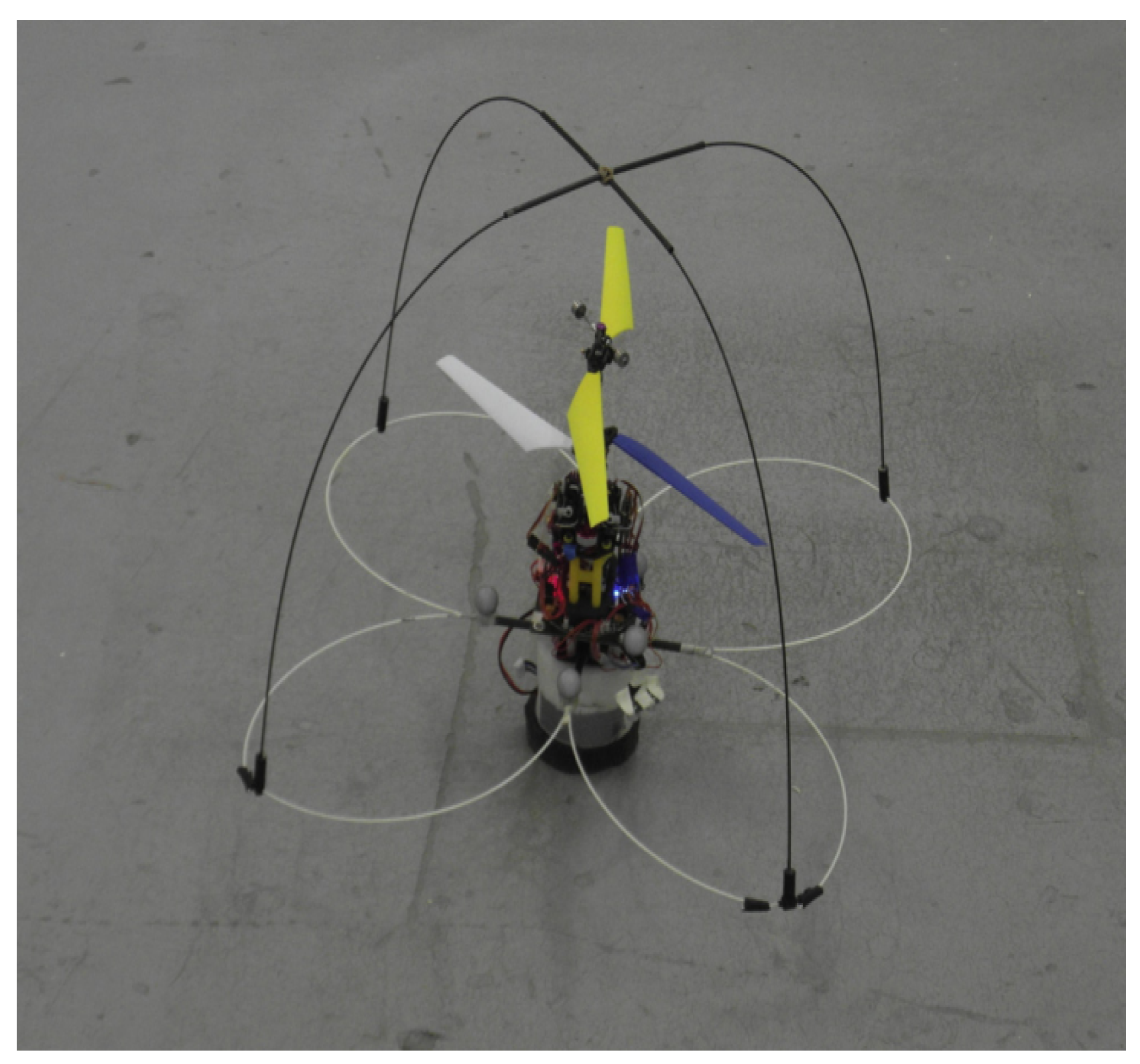
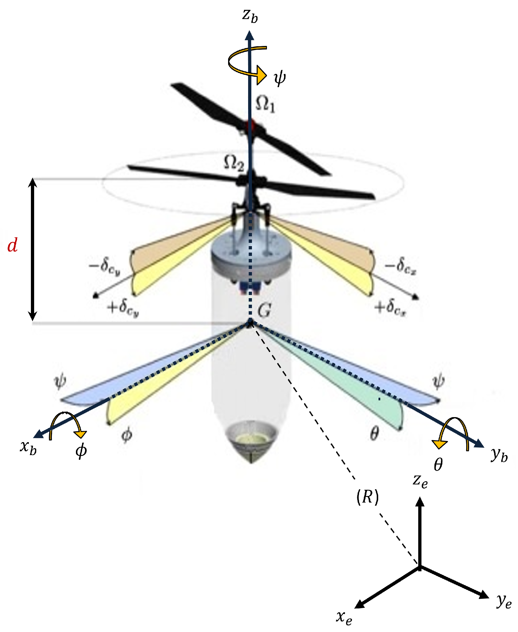
2. Coaxial Rotor Helicopter Modelling

To accurately capture the behavior of the coaxial rotor helicopter, its translatory dynamics about the x, y, and z axes along with the rotational dynamics along the roll, pitch, and yaw axes are modeled. This modeling approach is crucial for achieving stability, maneuverability, and reliable controllability of the helicopter during various flight tasks and operational scenarios.
The motion of the coaxial rotor in a three-dimensional space is analyzed by introducing two coordinate systems:  E ( x e , y e , z e )  and  B ( x b , y b , z b ) , which are represented by the Earth frame and the body frame, respectively. The body frame aligns with the coaxial rotor’s center of gravity, while the Earth frame serves as the stable reference frame. An illustration of the coaxial rotor helicopter with the frames of reference is presented in Figure 2.
The position and orientation of the coaxial rotor in the Earth frame are denoted as  P = [ x , y , z ] T , and  η = [ ϕ , θ , ψ ] T , respectively. These angles,  ϕ θ , and  ψ , represent the roll, pitch, and yaw rotations around the x, y, and z axes, respectively. The coaxial rotor’s position and rotation are governed through the control of thrust T and the application of three control torques  ( τ ϕ , τ θ , τ ψ ) . These control inputs empower the coaxial rotor to execute desired position and attitude changes. The transformation between the Earth frame  E ( x e , y e , z e )  and the body frame  B ( x b , y b , z b )  is elucidated by means of a rotation matrix, capturing the relationship between these two coordinate systems and provided as [4,33]
R = c o s θ c o s ψ s i n ϕ s i n θ c o s ψ c o s ϕ s i n ψ c o s ϕ i n θ c o s ψ + s i n ϕ s i n ψ c o s θ s i n ψ s i n ϕ s i n θ s i n ψ + c o s ϕ c o s ψ c o s ϕ s i n θ s i n ψ s i n ϕ c o s ψ s i n θ s i n ϕ c o s θ c o s ϕ c o s θ
Using Newton–Euler formulation, the dynamic model with neglecting the external disturbances can be described as [34]
m P ¨ = R T m g ( 0 , 0 , 1 ) T J η ¨ = Ψ η T τ C ( η , η ˙ ) η ˙
where m denotes the vehicle mass, g is the gravitational acceleration, and the symmetric and positive definite matrix containing the inertia parameters  I x I y , and  I z  is denoted as J. The term  C ( η , η ˙ )  represents the Coriolis term, which accounts for the coupling effects between the rotational and translational motions of the vehicle [35]. Finally,  Ψ η  represents the Euler parameter, which is provided by
Ψ η = 1 0 s θ 0 c ϕ s ϕ c θ 0 s ϕ c ϕ c θ
The thrust T is generated by the two rotors and can be expressed in terms of the rotor angular speeds  Ω 1  and  Ω 2 , along with the swash-plate incidence angles  δ c x  and  δ c y . The expression for thrust is defined as follows
T = T x T y T z = k β sin δ c y cos δ c x Ω 2 2 k β sin δ c x Ω 2 2 k α Ω 1 2 + k β cos δ c x cos δ c y Ω 2 2
where  k α  and  k β  are positive coefficients related to rotor aerodynamics. The torque vector  τ  is produced due to the separation between the center of mass and the rotor hubs and can be represented as
τ = τ ϕ τ θ τ ψ = d k β sin δ c x Ω 2 2 d k β sin δ c y cos δ c x Ω 2 2 γ 1 Ω 1 2 γ 2 Ω 2 2
where  γ 1  and  γ 2  denote the positive yaw aerodynamic coefficients and d is the distance between the center of gravity and the center of rotation of the lower rotor.
Utilizing Equations (2)–(5), we can derive the coaxial rotor model in the Earth frame  E ( x e , y e , z e )  as follows [31]
x ¨ = ( c ϕ s θ c ψ + s ϕ s ψ ) ( k α Ω 1 2 + k β cos δ c x cos δ c y Ω 2 2 ) m y ¨ = ( c ϕ s θ s ψ s ϕ c ψ ) ( k α Ω 1 2 + k β cos δ c x cos δ c y Ω 2 2 ) m z ¨ = ( c ϕ c θ ) ( k α Ω 1 2 + k β cos δ c x cos δ c y Ω 2 2 ) m g ϕ ¨ = I y I z I x θ ˙ ψ ˙ d k β sin δ c x Ω 2 2 I x θ ¨ = I z I x I y ϕ ˙ ψ ˙ + d k β sin δ c y cos δ c x Ω 2 2 I y ψ ¨ = I x I y I z ϕ ˙ θ ˙ + γ 1 Ω 1 2 γ 2 Ω 2 2 I z
Remark 1.
From a practical standpoint, it is assumed that the swash-plate incidence angles  δ c x  and  δ c y  are small. Under such assumptions, the nonlinear components can be approximated as  cos δ c x cos δ c y 1  and  sin δ c x δ c x ,  sin δ c y δ c y [4]. Consequently, the lateral effects induced by  T x  and  T y  in Equation (4) can be considered insignificant when compared to the primary thrust component  T z .
Control over these parameters is achieved by utilizing input signals  Ω 1 Ω 2 δ c x , and  δ c y , which can be obtained by applying an inverse transformation to Equations (4) and (5) and under Remark 1. The expressions for the input signals are as follows:
Ω 1 2 = γ 2 T z k β τ ψ k α γ 2 + k β γ 1 , Ω 2 2 = γ 1 T z k α τ ψ k α γ 2 + k β γ 1 , δ c x = τ ϕ d k β Ω 2 2 , δ c y = τ θ d k β Ω 2 2 .
To ensure the controllability of the system, it is necessary to impose bounds on the Euler angles. Specifically, the roll angle  ϕ , the pitch angle  θ , and the yaw angle  ψ  should satisfy the following conditions:  ϕ < π 2 θ < π 2 , and  ψ < π . These bounds restrict the range of motion for the Euler angles and ensure that the system remains within a controllable region. By imposing these constraints, the system can be effectively controlled while maintaining the stability and maneuverability of the coaxial rotor vehicle.

Control Oriented Model Development

The developed coaxial rotor model in Equation (6) consists of two sets of interconnected nonlinear subsystems: (a) the position dynamics along x, y, and z axes and (b) the rotational dynamics along the  ϕ θ , and  ψ  angles. Each subsystem can be further categorized into three subsystems to represent the dynamics along each individual axis. The position dynamics can be represented as an under-actuated subsystem because it relies solely on the force  T z  for control. Control over the coaxial rotor’s rotational motion is achieved through the application of three torques,  τ ϕ τ θ , and  τ ψ . These inputs directly influence the orientation rates of the coaxial rotor. However, these inputs cannot directly influence the angular positions, leading to an under-actuated scenario.
To address this under-actuated nature, three virtual inputs, namely  u x u y , and  u z , are introduced. These virtual inputs serve the purpose of controlling the position of the coaxial rotor. By appropriately assigning values to  u x u y , and  u z , the desired position coordinates can be regulated despite the limitations of the available control inputs. These virtual inputs are chosen as
u x , u y , u z T = T z R ( 0 , 0 , 1 ) T g ( 0 , 0 , 1 ) T
The coaxial position and orientation, represented by  y i x , y , z , ϕ , θ , ψ , are selected as the outputs to be controlled. The desired position coordinates  x d y d z d , and the desired yaw angle  ψ d  are considered as inputs to the control system. Furthermore, we determine the desired angles  ϕ d  and  θ d , along with the desired magnitude of the force vector  T z , by utilizing Equation (9) based on the position subsystems group, as shown below: [12]
T z ϕ d θ d = u x 2 + u y 2 + ( u z + g ) 2 sin 1 [ 1 T z ( u x sin ψ d u y cos ψ d ) ] sin 1 [ 1 T z cos ϕ d ( u x cos ψ d + u y sin ψ d ) ]
This equation establishes a connection between the desired position and orientation values, with  u x u y , and  u z  corresponding to the x, y, and z subsystems, respectively. Incorporating Eqations (8) and (9) and taking into consideration external disturbances that may influence the coaxial model, like wind, as well as the unmodeled nonlinearities represented by  h i ( t ) , the dynamic model presented in (9) can be expressed as follows:
x ˙ i 1 = x i 2 , x ˙ i 2 = f i ( X ) + b i u i ( t ) + h i ( t ) , i { x , y , z , ϕ , θ , ψ }
where  X = [ x x 1 , x x 2 , , x ψ 1 , x ψ 2 ] T = [ x , x ˙ , y , y ˙ , z , z ˙ , ϕ , ϕ ˙ , θ , θ ˙ , ψ , ψ ˙ ] T  is the total state vector of the coaxial rotor and can denoted as  x i = [ x i 1 , x i 2 ] T R 2 , where  x i 1  and  x i 2  represent the local state vector of each subsystem. The control input for each subsystem is represented by  u i u x , u y , u z , u ϕ , u θ , u ψ . Moreover,  f i ( X )  and  b i  correspond to the nonlinear dynamic functions and the control input gains, respectively. In order to create a controller with a straightforward structure, minimizing computational complexity for ease of real-time implementation, we suggest a mathematical manipulation of the dynamic model (6) that is illustrated in Equations (11)–(13). This manipulation aims to yield a single nonlinear function, denoted as  Ψ i ( X , t ) , for each subsystem i, which encompasses both the dynamic nonlinearities and external disturbances.
By left-multiplying the second equation of (10) by  b i 1 , we can express it as
b i 1 x ˙ i 2 = b i 1 f i ( X ) + b i 1 h i ( t ) + u i ( t )
Adding  x ˙ i 2 b i 1 x ˙ i 2  to both sides yields
x ˙ i 2 = Ψ i ( X , t ) + u i ( t )
where the total nonlinear dynamic function with disturbances  Ψ i ( X , t )  takes the following expression
Ψ i ( X , t ) = ( 1 b i 1 ) x ˙ i 2 + b i 1 f i ( X ) + b i 1 h i ( t )
A simplified dynamic model was derived in (13). This model aims to facilitate the implementation of a controller that is both straightforward and uncomplicated. Moreover, our goal was to showcase the efficacy of our control strategy in addressing a range of challenges, encompassing unknown dynamics, uncertainties, and disturbances collectively denoted as  Ψ i ( X , t ) .
Consequently, the coaxial model (10) can be reformulated using the following adjusted state equations
x ˙ i 1 = x i 2 , x ˙ i 2 = Ψ i ( X , t ) + u i ( t ) , y i = x i 1 .
In the context of a coaxial rotor system described by Equation (14), the aim is now to design a control law  u i  using the proposed optimal model-free scheme and achieve precise tracking of desired paths for both position and attitude variables ( y i ).

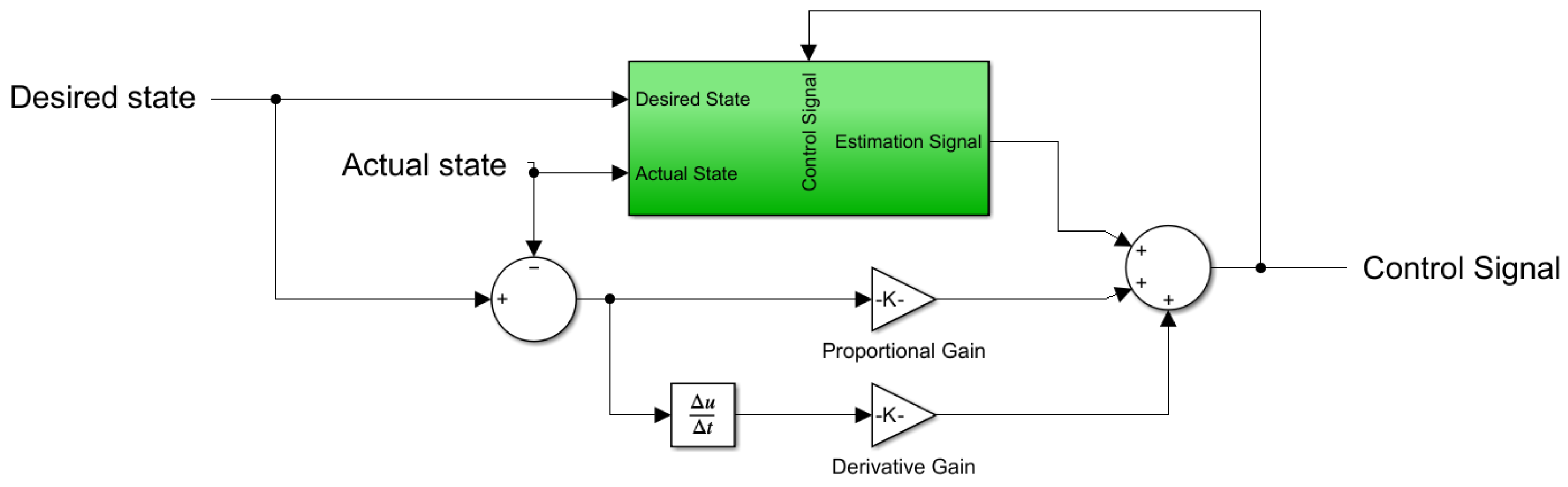
3. Robust Nonlinear Controller

In this section, a model-free controller for the path-tracking task while ensuring performance optimization, stability, and robust control is proposed. The main objectives can be summarized as follows:
  • Develop a direct control structure based on local measurements, eliminating the need for prior knowledge of the system’s dynamic model.
  • Ensure that the proposed control strategy drives the tracking error to finite-time convergence in the closed-loop system in the presence of disturbances.
  • Enhance the performance of the controller by incorporating a metaheuristic algorithm to optimize the control parameters and improve robustness.
To address these objectives, a model-free control approach based on terminal sliding mode is now proposed. The above discussion covers aspects of the optimization design in the closed-loop illustrated in Figure 3.

3.1. Model-Free Control Based on Terminal Sliding Mode

The design of the model-free control strategy is discussed in this section. First, we establish some lemmas to be used for stability analysis.
Lemma 1
((Cauchy–Schwarz inequality) [36]). For any  α n  with  n = 1 , 2 , , m  and  0 < ϵ 1 , then
α 1 + α 2 + α n ϵ α 1 ϵ + α 2 ϵ + α n ϵ
Lemma 2
([37]). A Lyapunov function that verifies the following inequality  V ˙ + λ 1 V + λ 2 V γ 0 , where  λ 1 > 0 ,  λ 2 > 0 , and  0 < γ < 1  are scalars, implies the existence of finite-time stability. The settling time can be expressed as
t f t 0 + 1 λ 1 ( 1 γ ) ln λ 1 V 1 γ t 0 + λ 2 λ 2
where  t 0  is an initial time.
The tracking error and its derivatives for the attitude and position path tracking of the coaxial rotor UAV can be defined as
e i = y i d y i e ˙ i = y ˙ i d x ˙ i 1 e ¨ i = y ¨ i d x ˙ i 2
where  y ˙ i d  and  y ¨ i d  represent the first and second derivatives of  y i d , respectively, and their values are assumed to be smooth, known, and bounded. By substituting Equation (15) into Equation (14), the dynamics of the coaxial rotor can be characterized by the tracking error equations as follows
e ¨ i y ¨ i d + Ψ i ( X , t ) + u i ( t ) = 0
From Equation (16), it ensures that the tracking errors converge to zero when a control law is defined in the following form
u i ( t ) = y ¨ i d + K P i e i + K D i e ˙ i Ψ i ( X , t )
Here,  K P i > 0  and  K D i > 0  are user-selected controller gains aimed at ensuring the closed-loop stability, as described by the following error equation
K P i e i + K D i e ˙ i + e ¨ i = 0
Thus, the tracking errors can converge to zero through linear control provided that the nonlinear function  Ψ i ( X , t )  is well-defined. However, inaccurate model information may cause instability and tracking failure. To overcome this drawback, we propose to develop a nonlinear estimation based on terminal sliding mode to approximate the value of the nonlinear function  Ψ i ( X , t )  as
Ψ ^ i ( X , t ) = Γ i S i β i s g n ( S i ) ϵ i S i λ i / c i
where  Γ i β i , and  ϵ i  are design parameters to be adjusted to control the weighting of the tracking error in relation to the sliding surface convergence. Additionally,  β i > Ψ i , where  .  represents the 1-norm.  λ i  and  c i  are positive odd integers ( λ i < c i ), and  S i  denotes the sliding surface, which can be defined as
S i = e i v x i 2
with  e i v  being a modified tracking error and its dynamic equation provided as
e ˙ i v = Γ i S i β i s g n ( S i ) ϵ i S i λ i / c i u i ( t )
The time derivative of (21) is
S ˙ i = e ˙ i v x ˙ i 2 = Γ i S i β i s g n ( S i ) ϵ i S i λ i / c i u i ( t ) x ˙ i 2 = Γ i S i β i s g n ( S i ) ϵ i S i λ i / c i Ψ i ( X , t ) Ψ ˜ i = Ψ ^ i Ψ i
where  Ψ ˜ i  is the estimation error. Using the estimation of  Ψ i ( X , t ) , a model-free control-based terminal sliding mode (MFC-TSM) can be proposed as
u i ( t ) = y ¨ i d + K P i e i + K D i e ˙ i Ψ ^ i ( X , t )
The proposed control strategy, as defined in Equation (23), offers a simplified mathematical structure that eliminates the need for complex calculations by utilizing local measurements. This design choice enhances the computational efficiency of the controller. The control structure, depicted in Figure 4, visualizes the components and interactions of the proposed controller. The stability analysis of the proposed controller is provided below, ensuring the robustness and reliability of the control system.
Theorem 1.
By considering the dynamic model (13) with the proposed control law in (23) and the estimation term in (19), it can be demonstrated that the position and attitude tracking errors  e i  of the coaxial rotor converge to zero, leading to asymptotic stability of the closed-loop system.
Proof. 
A Lyapunov candidate function V is defined as
V = i { x , y , z , φ , θ , ψ } V i
where  V i  is the subsystem stability function, with
V i = 1 2 S i 2
The time derivative of the Lyapunov function V can be provided as
V ˙ i = S i S ˙ i
By substituting (22) into (25),  V ˙ i  becomes
V ˙ i = S i ( Γ i S i β i s g n ( S i ) ϵ i S i λ i / c i Ψ i ( X , t ) ) = Γ i S i 2 β i S i s g n ( S i ) ϵ i S i ( λ i + c i ) / c i Ψ i ( X , t ) S i Γ i S i 2 β i S i ϵ i S i ( λ i + c i ) / c i + Ψ i ( X , t ) S i Γ i S i 2 ϵ i S i ( λ i + c i ) / c i
Using Lemma 2,  V ˙  can be expressed as:
V ˙ i 2 Γ i V i 2 ( λ i + c i ) / 2 c i ) ϵ i V ( λ i + c i ) / 2 c i )
From (28), (24), and Lemma 2, it can thus be deduced that the proposed MFC-TSM controller ensures finite-time convergence [38]. Thus, the stability of the coaxial rotor closed-loop system is guaranteed and the variables  e i , e ˙ i , and  u i  are bounded with respect to the design parameters  Γ i , β i , ϵ i , λ i , and  c i . □
The use of the discontinuous function sgn(.) in the control law induces chattering, causing vibrations in the system. To mitigate this effect, various methods have been proposed in the literature [39,40,41]. In our study, we adopt a tan sigmoid function as an alternative to the sign function to reduce chattering.
The performance of the system in the tracking path task is highly dependent on the optimal selection of the design parameters, namely  K P i K D i Γ i β i , and  ϵ i , as indicated in Equations (19) and (23). To achieve maximum performance, an automated tuning method is proposed in the form of an accelerated particle swarm optimization (APSO) algorithm.

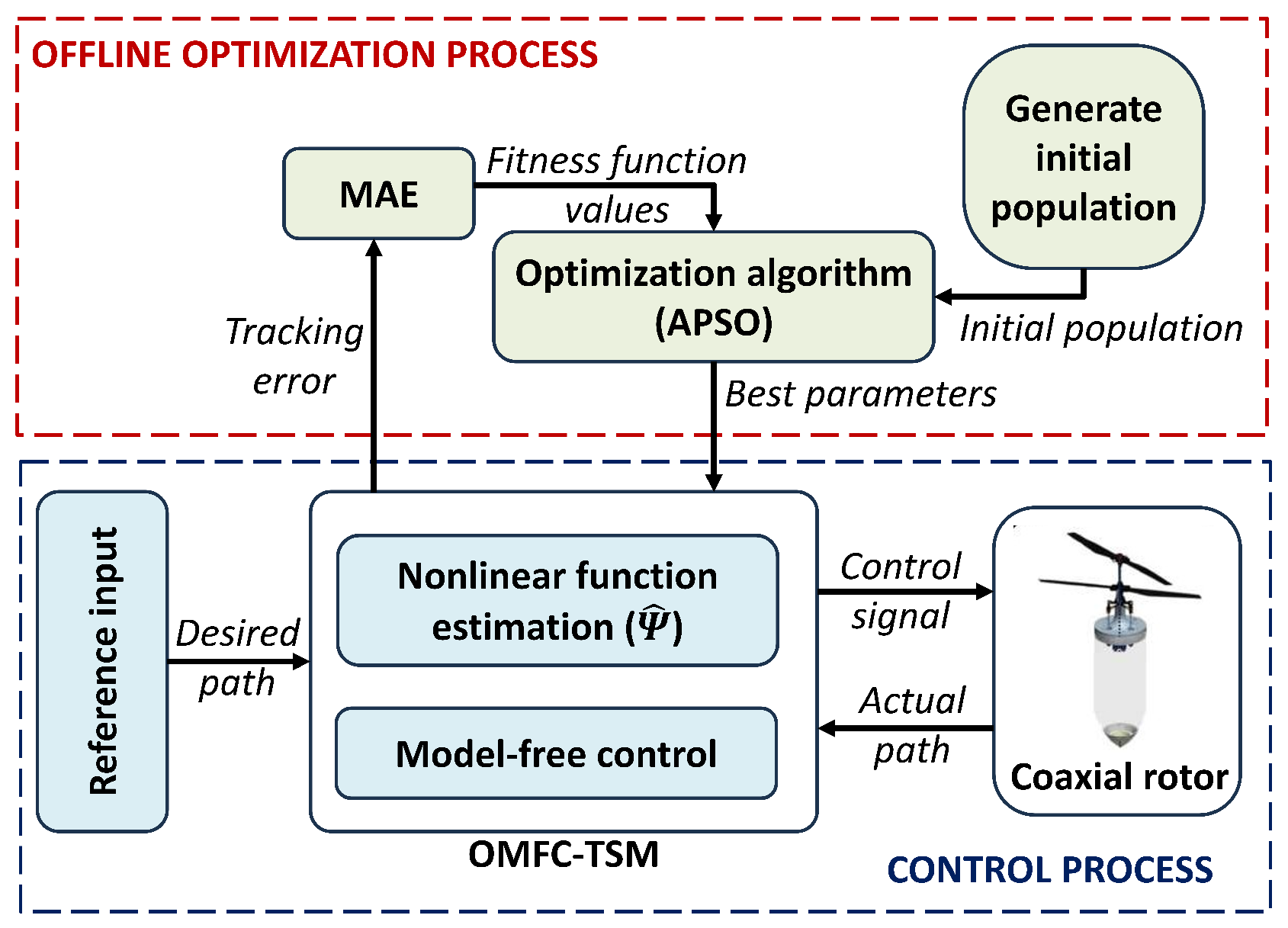
3.2. Optimization of Control Parameters

In this section, the optimization of the control parameters using APSO (adaptive particle swarm optimization) [42] is discussed. It is important to note that the proposed control law in Equations (19) and (23) becomes optimal when the parameters  K P i ,   K D i ,   Γ i ,   β i ,   ϵ i  can be selected optimally and it needs to satisfy stability criteria (28).
To describe the procedure of the particle swarm optimization (PSO) algorithm, we define  ρ μ ( t ) K P i ,   K D i ,   Γ i ,   β i ,   ϵ i  as the position vector and  v μ ( t )  as the velocity vector of particle  μ . The updated velocity vector  v μ ( t + 1 )  is determined based on the current global best value  G = min J ρ μ ( t )  as follows [42]
v μ ( t + 1 ) = w v μ ( t ) + γ t ( ϵ 1 / 2 ) + C 1 r 1 ρ μ * ρ μ ( t ) + C 2 r 2 G ρ μ ( t )
Here,  ϵ [ 0 , 1 ]  represents a random variable. The cognition decreasing function is defined as  γ t = γ 0 e λ t , where  γ 0 = 0.5  and  0 < λ < 1 . The inertia weight is denoted by w, while  C 1  and  C 2  represent the cognition learning and social learning factors, respectively. Additionally,  r 1 , r 2 [ 0 , 1 ]  are generated random numbers. The new position is then computed as
ρ μ ( t + 1 ) = ρ μ ( t ) + v μ ( t + 1 )
Below is the step-by-step procedure for employing the APSO to obtain the optimal parameters for the proposed control law:
  • Step 1: Initialize the following parameters:
  • Population size: The number of swarms in the population.
  • Number of iterations: The maximum number of iterations the algorithm will perform.
  • Step size t: The step size is used for generating new parameter values during pollination operations.
These parameters are crucial for controlling the behavior of the APSO and must be appropriately set to ensure effective optimization.
  • Step 2: Generate the initial feasible solutions according to the search space set from experience, with the same size as the dimensional problem. For each initial solution, compute mean absolute error (MAE), which is used as the fitness function and denoted by  J i , as follows:
J i = j = 1 N e i N
Here, jth is a sampling time, and N is the sample size.
Proposition 1.
Based on the observation from Equation (6) that the position subsystems have the same dimensions as the rotation subsystems, we propose to introduce two global objective functions during the optimization process. These objective functions are designed to optimize the performance of both the position and rotation subsystems simultaneously.
For the position objective function, denoted as  J p , we consider the summation of individual objective terms  J i  for each position component (x, y, and z) divided by 3 to ensure a balanced contribution. Mathematically, it can be expressed as  J p = i x , y , z J i / 3 .  Similarly, for the rotation objective function, denoted as  J r , we consider the sum of individual objective terms  J i  for each rotation component ( ϕ θ , and  ψ ) divided by 3. It can be formulated as  J r = i ϕ , θ , ψ J i / 3 .
  • Step 3: Update the velocity and position of each particle using the APSO algorithm. This involves adjusting the control parameters based on the particle’s previous position, velocity, and its best-known position and the best-known position in the entire swarm.
  • Step 4: Repeat steps 2 and 3 for a predefined number of iterations or until a convergence criterion is met. Once the optimization process is complete, the control parameters of the particle with the best fitness are considered as the tuned proposed parameters.
It is important to note that the success of the tuning depends on the characteristics of the system being controlled. Additionally, the search space should be well taken to avoid instability or undesirable behavior in the control system during the tuning process.

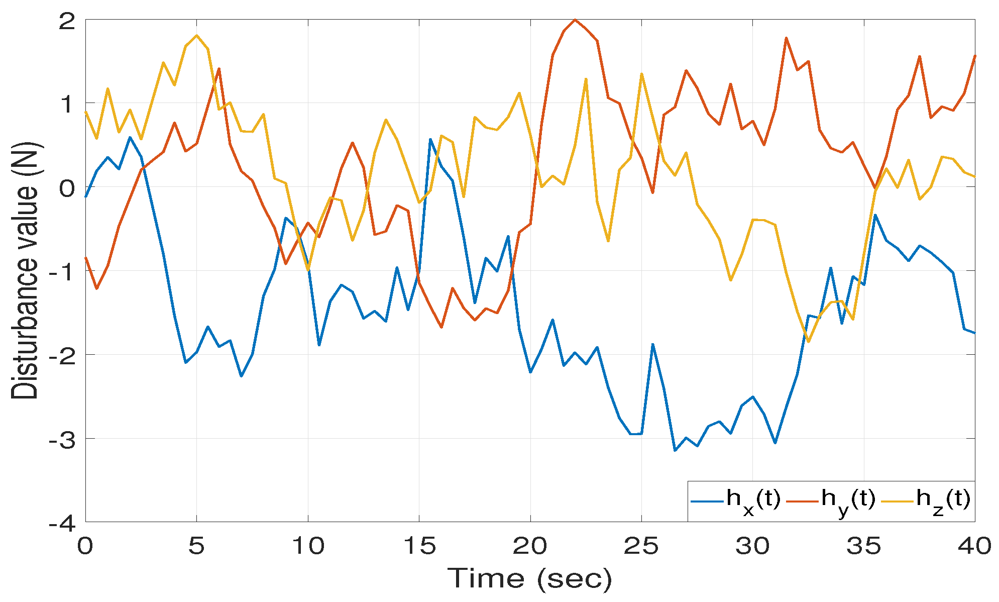
4. Results and Discussion

The performance of the proposed OMFC-TSM scheme for the coaxial rotor was evaluated by numerical simulations on the Matlab/Simulink platform. The simulations were carried out for various reference signals provided for the path-tracking task. The initial states for the estimator were selected as  y i 0 = 0  for  i x , y , z , ϕ , θ , ψ . The physical parameters of the coaxial rotor used in the simulations can be found in Table 1 [4]. To optimize the designed controller, the APSO algorithm was configured with a swarm size of  n = 10 , cognitive parameter  C 1 = 2 , social parameter  C 2 = 2 , and inertia weight  w = 2 . The optimization process was iterated for a total of 100 iterations, allowing the algorithm to converge and find optimal controller parameters.

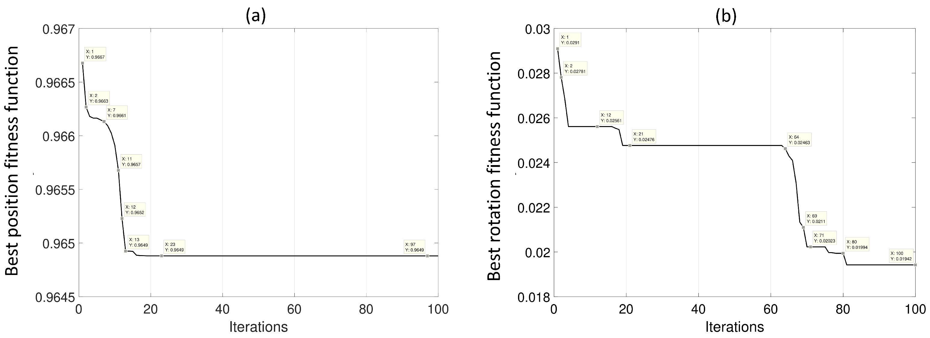
4.1. APSO-Based Parameter Tuning

In this study, the coaxial rotor model with the proposed controller was simulated for 100 iterations to achieve statistically reliable outcomes from the accelerated particle swarm optimization (APSO) algorithm. The main objective was to optimize the parameters of the proposed controller by minimizing the cost function J, while adhering to the stability condition, within the bounded search space  μ i [ μ min i , μ max i ] . To ensure robust optimization results, the optimization algorithm relies on generating random initial values during its operation.
Figure 5 presents the convergence behavior of the optimization process for the position and rotation subsystems.
The graph illustrates the progress of the cost function J over the iterations, demonstrating the improvement achieved by the APSO algorithm in finding the optimal solution. The best iteration provides valuable insights into the convergence behavior and represents the statistical outcome of the optimization process. Figure 5 clearly demonstrates the effectiveness of the accelerated particle swarm optimization (APSO) algorithm in fine-tuning the parameters of the proposed controller. The convergence rate is very high, as evidenced by the achieved minimized values of  J p = 0.9675  m and  J r = 0.0194  rad within a mere 100 iterations. This highlights the exceptional performance of the APSO algorithm in efficiently addressing the optimization problem associated with the controller design. The optimized parameter values obtained through the optimization process are presented in Table 2.
To show the effectiveness of the proposed APSO-based optimally tuned OMFC-TSM, comparison studies with two OMFC-TSM controllers without any optimal tuning were carried out for square path defined as
y x d = 0 m f o r 20 s < t < 35 s e l s e 2 m y y d = 2 m f o r 10 s < t < 30 s e l s e 0 m y z d = 3 m y ψ d = 0 rad
To ensure the boundedness of all closed-loop system signals, the desired trajectory was filtered in order to make it smooth. The gains of such controllers were arbitrarily selected but ensured convergence and stability. The 3D-path-tracking comparison results for such conditions are presented in Figure 6. The maximum values of the tracking error  M a x | e j | j = x , y , z  for all three controllers show that the proposed APSO-based optimally tuned OMFC-TSM outperforms the other two non-optimal controllers.
These optimized parameters play a crucial role in significantly enhancing the performance of the proposed controller, resulting in improved trajectory tracking accuracy and system stability. The successful optimization process further reinforces the effectiveness and reliability of the proposed approach in addressing the trajectory tracking issue for the coaxial rotor system.

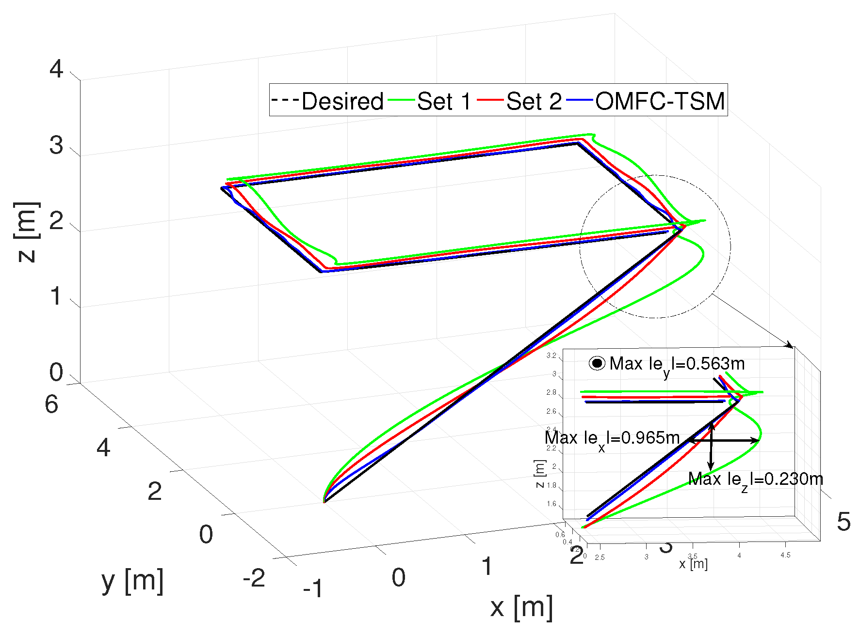
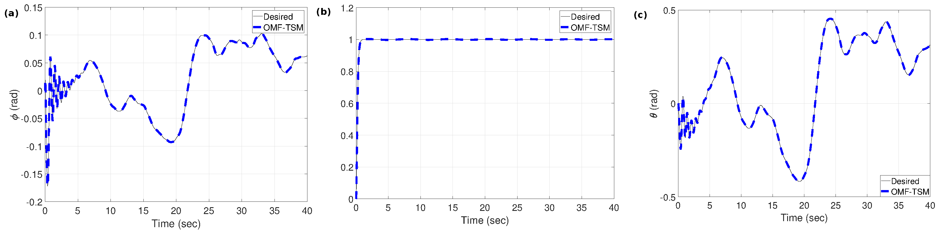
4.2. Performance Evaluation of APSO-Tuned OMFC-TSM Controller

The performance of the proposed APSO-tuned OMFC-TSM controller was then evaluated in the presence of external disturbances. The disturbances  h j  affecting each of the translational axes are selected as random bounded disturbances reflecting real flying scenarios in which wind speed remains unpredictable and presented in Figure 7. Further, the selection of disturbance profiles is aimed at encompassing the primary nonlinearities affecting the coaxial system.
The desired trajectory for the path tracking problem was defined as
y x d = 4 s i n ( t ) m y y d = 4 c o s ( t ) m y z d = 1 m y ψ d = 1 r a d
The attitude tracking performance of the proposed OMFC-TSM controller under the effect of disturbances is shown in Figure 8. It can be seen that, although initial oscillations are observed owing to the presence of wind disturbances, the proposed controller ensures convergence of tracking error and maintains stability.
The control inputs  Ω 1 , Ω 2 , δ c x , δ c y  generated by the OMFC-TSM controller for stabilizing the attitude and position subsystem in the presence of disturbances are shown in Figure 9.
To evaluate the robustness of the design approach, the OMFC-TSM has been compared with two well-known approaches; the PID controller and TDEC controller were designed according to [43,44]. The 3D trajectory tracking performance of all the controllers is shown in Figure 10.
It can be seen in Figure 10 that the TDEC and PID can track the desired path under the disturbances, but the best trajectory tracking can only be achieved with MFC-TSM. The PID controller exhibits bad tracking performance. Meanwhile, Figure 9 illustrates the behavior of the control inputs, indicating the success of the designed controller approach in achieving the desired trajectory despite the presence of external disturbances. The behavior of the sliding manifolds, depicted in Figure 11, aligns with expectations, demonstrating convergence to zero for all sliding manifolds. It is evident that, while all states asymptotically approach their desired values, the associated sliding manifolds also converge to zero. This observation serves to test and validate Equations (20)–(22). Furthermore, the simulation results demonstrate that incorporating continuous functions into the controller design effectively reduces chattering, mitigating its detrimental effects on systems. This improvement is valuable for practical applications, while retaining the finite-time convergence feature.
To provide a comprehensive evaluation of the proposed controllers, a detailed quantitative comparison was conducted for both the position and attitude subsystems. This comparison aimed to assess the performance using widely recognized criteria, including mean absolute error (MAE), root mean square error (RMSE), and maximum absolute error (MaxAE). The results of the comparison are summarized in Table 3, which reveals that the proposed approach outperforms the other techniques for both position and rotational subsystems.
The proposed OMFC-TSM control approach thus achieves high performance, as evidenced by the quantitative results, offers advantages of model-free design and reduced complexity, and can be easily implemented in real-time trajectory tracking control of coaxial rotor UAVs.

5. Conclusions

This paper presents a robust model-free controller for trajectory tracking of a coaxial rotor, addressing the limitations of model-based approaches. By combining model-free control (MFC) and terminal sliding mode (TSM) control, the proposed method effectively estimates the unknown dynamic functions of the coaxial rotor. The control design is validated using the Lyapunov theory, ensuring the stability of the system. The control parameters are tuned through an optimization problem solved by an accelerated particle swarm optimization (APSO) algorithm, optimizing tracking performance while maintaining stability. One of the key advantages of the proposed approach is its simplicity, with a relatively simple control structure and low-complexity design conditions. This simplicity, along with the model-free and smooth control signals, enhances its applicability in real-time coaxial rotor systems. The effectiveness of the proposed approach is demonstrated through comparative analysis with other existing methods. Our upcoming efforts will concentrate on implementing and validating the proposed control strategy in actual coaxial rotor applications. This will offer valuable insights into its performance and robustness in practical scenarios. Additionally, we are interested in addressing the issue of control signal saturation, which has the potential to cause instability and chattering.

Author Contributions

Conceptualization, H.E.G., C.S. and J.J.R.; methodology, H.E.G. and C.S.; software, H.E.G.; writing—original draft preparation, H.E.G. and C.S.; writing—review and editing, H.E.G., C.S. and J.J.R. All authors have read and agreed to the published version of the manuscript.

Funding

This research has been done in the framework of the RITMEA project, funded by the French Regional Delegation for Research and Technology and was also supported by the French Ministry of Higher Education and Research, and the French National Center for Scientific Research.

Data Availability Statement

The data is contained within the article.

Acknowledgments

The authors gratefully acknowledge the support of the French National Research Agency, the French Regional Delegation for Research and Technology, the French Ministry of Higher Education and Research, and the French National Center for Scientific Research.

Conflicts of Interest

The authors declare that the research was conducted without any commercial or financial relationships that could be construed as a potential conflict of interest.

References

  1. Kumar, V.; Michael, N. Opportunities and challenges with autonomous micro aerial vehicles. Int. J. Robot. Res. 2012, 31, 1279–1291. [Google Scholar] [CrossRef]
  2. Ouyang, F.; Cheng, H.; Lan, Y.; Zhang, Y.; Yin, X.; Hu, J.; Peng, X.; Wang, G.; Chen, S. Automatic delivery and recovery system of Wireless Sensor Networks (WSN) nodes based on UAV for agricultural applications. Comput. Electron. Agric. 2019, 162, 31–43. [Google Scholar] [CrossRef]
  3. Lippiello, V.; Fontanelli, G.A.; Ruggiero, F. Image-Based Visual-Impedance Control of a Dual-Arm Aerial Manipulator. IEEE Robot. Autom. Lett. 2018, 3, 1856–1863. [Google Scholar] [CrossRef]
  4. Mokhtari, M.R.; Cherki, B.; Braham, A.C. Disturbance observer based hierarchical control of coaxial-rotor UAV. ISA Trans. 2017, 67, 466–475. [Google Scholar] [CrossRef] [PubMed]
  5. Kim, H.J.; Shim, D.H. A flight control system for aerial robots: Algorithms and experiments. Control Eng. Pract. 2003, 11, 1389–1400. [Google Scholar] [CrossRef]
  6. Mettler, B. Identification Modeling and Characteristics of Miniature Rotorcraft; Springer Science & Business Media: Berlin/Heidelberg, Germany, 2013. [Google Scholar]
  7. Artale, V.; Milazzo, C.L.; Orlando, C.; Ricciardello, A. Comparison of GA and PSO approaches for the direct and LQR tuning of a multirotor PD controller. J. Ind. Manag. Optim. 2017, 13, 2067. [Google Scholar] [CrossRef]
  8. Drouot, A.; Zasadzinski, M.; Souley-Ali, H.; Richard, E.; Boutayeb, M. Two robust static output feedback Hinf control architectures for a Gun Launched Micro Aerial Vehicle. In Proceedings of the 21st Mediterranean Conference on Control and Automation, Chania, Crete, 25–28 June 2013; pp. 185–190. [Google Scholar]
  9. Joel, N.C.; Djalo, H.; Aurelien, K. Robust control of UAV coaxial rotor by using exact feedback linearization and PI-observer. Int. J. Dyn. Control 2019, 7, 201–208. [Google Scholar] [CrossRef]
  10. Espinoza, E.S.; Garcia, O.; Lugo, I.; Ordaz, P.; Malo, A.; Lozano, R. Modeling and sliding mode control of a micro helicopter-airplane system. J. Intell. Robot. Syst. 2014, 73, 469–486. [Google Scholar] [CrossRef]
  11. Drouot, A.; Richard, E.; Boutayeb, M. An approximate backstepping based trajectory tracking control of a gun launched micro aerial vehicle in crosswind. J. Intell. Robot. Syst. 2013, 70, 133–150. [Google Scholar] [CrossRef]
  12. Drouot, A.; Richard, E.; Boutayeb, M. Hierarchical backstepping-based control of a Gun Launched MAV in crosswinds: Theory and experiment. Control Eng. Pract. 2014, 25, 16–25. [Google Scholar] [CrossRef]
  13. Zhang, J.; Ren, Z.; Deng, C.; Wen, B. Adaptive fuzzy global sliding mode control for trajectory tracking of quadrotor UAVs. Nonlinear Dyn. 2019, 97, 609–627. [Google Scholar] [CrossRef]
  14. Zhang, H.; Zeng, Z.; Yu, C.; Jiang, Z.; Han, B.; Lian, L. Predictive and sliding mode cascade control for cross-domain locomotion of a coaxial aerial underwater vehicle with disturbances. Appl. Ocean Res. 2020, 100, 102183. [Google Scholar] [CrossRef]
  15. Zeghlache, S.; Mekki, H.; Bouguerra, A.; Djerioui, A. Actuator fault tolerant control using adaptive RBFNN fuzzy sliding mode controller for coaxial octorotor UAV. ISA Trans. 2018, 80, 267–278. [Google Scholar] [CrossRef] [PubMed]
  16. Lv, Z.; Wu, Y.; Zhao, Q.; Sun, X.M. Design and Control of a Novel Coaxial Tilt-Rotor UAV. IEEE Trans. Ind. Electron. 2021, 69, 3810–3821. [Google Scholar] [CrossRef]
  17. Fliess, M.; Join, C. Model-free control. Int. J. Control 2013, 86, 2228–2252. [Google Scholar] [CrossRef]
  18. Al Younes, Y.; Drak, A.; Noura, H.; Rabhi, A.; El Hajjaji, A. Robust model-free control applied to a quadrotor UAV. J. Intell. Robot. Syst. 2016, 84, 37–52. [Google Scholar] [CrossRef]
  19. Barth, J.M.; Condomines, J.P.; Moschetta, J.M.; Cabarbaye, A.; Join, C.; Fliess, M. Full model-free control architecture for hybrid UAVs. In Proceedings of the 2019 American Control Conference (ACC), Philadelphia, PA, USA, 10–12 July 2019; pp. 71–78. [Google Scholar]
  20. Wang, H.; Ye, X.; Tian, Y.; Zheng, G.; Christov, N. Model-free–based terminal SMC of quadrotor attitude and position. IEEE Trans. Aerosp. Electron. Syst. 2016, 52, 2519–2528. [Google Scholar] [CrossRef]
  21. Li, Z.; Ma, X.; Li, Y. Model-free control of a quadrotor using adaptive proportional derivative-sliding mode control and robust integral of the signum of the error. Int. J. Adv. Robot. Syst. 2018, 15, 1729881418800885. [Google Scholar] [CrossRef]
  22. Bouzid, Y.; Siguerdidjane, H.; Bestaoui, Y. Generic dynamic modeling for multirotor VTOL UAVs and robust Sliding Mode based Model-Free Control for 3D navigation. In Proceedings of the 2018 International Conference on Unmanned Aircraft Systems (ICUAS), Dallas, TX, USA, 12–15 June 2018; pp. 970–979. [Google Scholar] [CrossRef]
  23. Glida, H.E.; Abdou, L.; Chelihi, A.; Sentouh, C.; Hasseni, S.E.I. Optimal model-free backstepping control for a quadrotor helicopter. Nonlinear Dyn. 2020, 100, 3449–3468. [Google Scholar] [CrossRef]
  24. Fu, C.; Hong, W.; Lu, H.; Zhang, L.; Guo, X.; Tian, Y. Adaptive robust backstepping attitude control for a multi-rotor unmanned aerial vehicle with time-varying output constraints. Aerosp. Sci. Technol. 2018, 78, 593–603. [Google Scholar] [CrossRef]
  25. Wang, G.; Yang, W.; Zhao, N.; Shen, Y.; Wang, C. An approximation-free simple controller for uncertain quadrotor systems in the presence of thrust saturation. Mechatronics 2020, 72, 102450. [Google Scholar] [CrossRef]
  26. Bounemeur, A.; Chemachema, M.; Essounbouli, N. Indirect adaptive fuzzy fault-tolerant tracking control for MIMO nonlinear systems with actuator and sensor failures. ISA Trans. 2018, 79, 45–61. [Google Scholar] [CrossRef]
  27. Zeghlache, S.; Djerioui, A.; Benyettou, L.; Benslimane, T.; Mekki, H.; Bouguerra, A. Fault tolerant control for modified quadrotor via adaptive type-2 fuzzy backstepping subject to actuator faults. ISA Trans. 2019, 95, 330–345. [Google Scholar] [CrossRef] [PubMed]
  28. Chekakta, Z.; Zerikat, M.; Bouzid, Y.; Koubaa, A. Adaptive fuzzy model-free control for 3D trajectory tracking of quadrotor. Int. J. Mechatron. Autom. 2020, 7, 134–146. [Google Scholar] [CrossRef]
  29. Camci, E.; Kripalani, D.R.; Ma, L.; Kayacan, E.; Khanesar, M.A. An aerial robot for rice farm quality inspection with type-2 fuzzy neural networks tuned by particle swarm optimization-sliding mode control hybrid algorithm. Swarm Evol. Comput. 2018, 41, 1–8. [Google Scholar] [CrossRef]
  30. Glida, H.E.; Abdou, L.; Chelihi, A.; Sentouh, C.; Perozzi, G. Optimal model-free fuzzy logic control for autonomous unmanned aerial vehicle. Proc. Inst. Mech. Eng. Part G J. Aerosp. Eng. 2022, 236, 952–967. [Google Scholar] [CrossRef]
  31. Wei, Y.R.; Deng, H.B.; Pan, Z.H.; Li, K.W.; Chen, H. Research on a combinatorial control method for coaxial rotor aircraft based on sliding mode. Def. Technol. 2022, 18, 280–292. [Google Scholar] [CrossRef]
  32. Yan, K.; Chen, M.; Wu, Q. Neural network-based adaptive fault tolerant tracking control for unmanned autonomous helicopters with prescribed performance. Proc. Inst. Mech. Eng. Part G J. Aerosp. Eng. 2019, 233, 4350–4362. [Google Scholar] [CrossRef]
  33. Koehl, A.; Rafaralahy, H.; Boutayeb, M.; Martinez, B. Aerodynamic modelling and experimental identification of a coaxial-rotor UAV. J. Intell. Robot. Syst. 2012, 68, 53–68. [Google Scholar] [CrossRef]
  34. Glida, H.E.; Chelihi, A.; Abdou, L.; Sentouh, C.; Perozzi, G. Trajectory tracking control of a coaxial rotor drone: Time-delay estimation-based optimal model-free fuzzy logic approach. ISA Trans. 2022, 137, 236–247. [Google Scholar] [CrossRef] [PubMed]
  35. Nonami, K.; Kendoul, F.; Suzuki, S.; Wang, W.; Nakazawa, D. Autonomous Flying Robots: Unmanned Aerial Vehicles and Micro Aerial Vehicles; Springer Science & Business Media: Berlin/Heidelberg, Germany, 2010. [Google Scholar]
  36. Huang, X.; Lin, W.; Yang, B. Global finite-time stabilization of a class of uncertain nonlinear systems. Automatica 2005, 41, 881–888. [Google Scholar] [CrossRef]
  37. Yu, S.; Yu, X.; Shirinzadeh, B.; Man, Z. Continuous finite-time control for robotic manipulators with terminal sliding mode. Automatica 2005, 41, 1957–1964. [Google Scholar] [CrossRef]
  38. Zhihong, M.; Yu, X.H. Terminal sliding mode control of MIMO linear systems. IEEE Trans. Circuits Syst. Fundam. Theory Appl. 1997, 44, 1065–1070. [Google Scholar] [CrossRef]
  39. Jahanshahi, H.; Sari, N.N.; Pham, V.T.; Alsaadi, F.E.; Hayat, T. Optimal adaptive higher order controllers subject to sliding modes for a carrier system. Int. J. Adv. Robot. Syst. 2018, 15, 1729881418782097. [Google Scholar] [CrossRef]
  40. Yousefpour, A.; Jahanshahi, H.; Gan, D. Fuzzy integral sliding mode technique for synchronization of memristive neural networks. In Mem-Elements for Neuromorphic Circuits with Artificial Intelligence Applications; Elsevier: Amsterdam, The Netherlands, 2021; pp. 485–500. [Google Scholar]
  41. Zhou, S.S.; Jahanshahi, H.; Din, Q.; Bekiros, S.; Alcaraz, R.; Alassafi, M.O.; Alsaadi, F.E.; Chu, Y.M. Discrete-time macroeconomic system: Bifurcation analysis and synchronization using fuzzy-based activation feedback control. Chaos Solitons Fract. 2021, 142, 110378. [Google Scholar] [CrossRef]
  42. Yang, X.S. Nature-Inspired Optimization Algorithms; Elsevier: Amsterdam, The Netherlands, 2014. [Google Scholar]
  43. Hsia, T.S.; Lasky, T.; Guo, Z. Robust independent joint controller design for industrial robot manipulators. IEEE Trans. Ind. Electron. 1991, 38, 21–25. [Google Scholar] [CrossRef]
  44. Hasseni, S.E.I.; Abdou, L.; Glida, H.E. Parameters tuning of a quadrotor PID controllers by using nature-inspired algorithms. Evol. Intell. 2021, 14, 61–73. [Google Scholar] [CrossRef]
Figure 2. Coaxial rotor vehicle configuration [4].
Drones 07 00706 g002
Figure 3. Optimization of the proposed OMFC-TSM.
Drones 07 00706 g003
Figure 4. Structure of MFC-TSM.
Drones 07 00706 g004
Figure 5. (a) Convergence curve of the position objective function; (b) convergence curve of the rotation objective function.
Drones 07 00706 g005
Figure 6. Comparison of proposed OMF-TSM design with arbitrarily tuned controllers (Set 1 and Set 2);  M a x ( | . | )  is the maximum of absolute value function.
Drones 07 00706 g006
Figure 7. External disturbances  h j j = x , y , z  [30].
Drones 07 00706 g007
Figure 8. Coaxial rotor attitude tracking response. (a) Roll ( ϕ ) subsystem response; (b) yaw ( ψ ) subsystem response; (c) pitch ( θ ) subsystem response.
Drones 07 00706 g008
Figure 9. Coaxial rotor control signals using OMFC-TSM. (a) Control signals  δ c x  and  δ c x ; (b) control signals  Ω 1  and  Ω 2 .
Drones 07 00706 g009
Figure 10. 3D coaxial rotor trajectory tracking under wind effect.
Drones 07 00706 g010
Figure 11. Sliding manifolds using OMFC-TSM. (a) tracking sliding surface for position system; (b) Tracking sliding surface for rotation system.
Drones 07 00706 g011
Table 1. Parameters of the coaxial rotor.
ParametersValue
g9.81 m/s2
d0.0676 m
m0.41 kg
  I x 1.383 × 10 3  kg.m2
  I y 1.383 × 10 3  kg.m2
  I z 2.72 × 10 4  kg.m2
  k α 3.683 × 10 5  N/rad2 s2
  k β 3.776 × 10 5  N/rad2 s2
  γ 1 1.476 × 10 6  N.m/rad2 s2
  γ 2 1.326 × 10 6  N.m/rad2 s2
Table 2. Optimized parameters of OMFC-TSM obtained via APSO.
ith ControllerParameter Value
  K P   K D   Γ   β   ϵ
x9.4513.1833.9681.1592.174
y10.1352.6422.1540.9472.691
z13.2674.5484.9572.1531.983
  ϕ 5.6421.8461.6790.1871.872
  θ 3.9461.7511.7810.9241.781
  ψ 4.8731.9762.1151.5421.1371
Table 3. RMSE and MaxAE performance indexes.
CriterionController
PIDTDECOMFC-TSM
MAEPosition System0.25890.10620.0351
Rotation System0.00126.35  × 10 4 × 10 4
RMSEPosition System0.50750.29210.1740
Rotation System0.01990.01290.0129
MaxAEPosition System1.41151.02070.0788
Rotation System0.00480.00280.0030
Disclaimer/Publisher’s Note: The statements, opinions and data contained in all publications are solely those of the individual author(s) and contributor(s) and not of MDPI and/or the editor(s). MDPI and/or the editor(s) disclaim responsibility for any injury to people or property resulting from any ideas, methods, instructions or products referred to in the content.

