1. Introduction
With the advancement of computer and sensor technology, UGVs find applications in various domains, including military operations and reconnaissance, security surveillance, search and rescue missions, logistics and delivery, and industrial automation. The odometry task, as a crucial component of the UGV framework, has been studied for decades but still presents challenges such as drift of pose estimation and the fusion of data from different sensors [
1]. Our work primarily revolves around enhancing odometry estimation accuracy and optimizing multisensory fusion.
Traditional odometry methods typically rely on hand-crafted features to estimate relative pose and have achieved high accuracy [
2]. However, these methods depend on human experience and lack adaptability in challenging scenarios. Recently, odometry methods based on deep neural networks have gained growing interest. Compared to traditional odometry methods, deep odometry methods offer several advantages: (1) High-dimensional features extracted by deep learning demonstrate robustness in the face of challenging scenarios; (2) Deep odometry methods do not require complex parameter calibration and geometric transformations; (3) Deep odometry methods can continuously learn and adapt to new scenes as their datasets expand.
In the face of complex environments, it is necessary for UGV to embrace multisensory fusion to enhance robustness [
3]. These sensors include cameras, lidar, and inertial measurement units (IMUs). In recent years, numerous studies have been proposed to deal with the odometry task using these different sensors. Monocular cameras, being small-sized and cost-effective, provide rich pixel information. However, they heavily rely on sufficient visible light and struggle to extract range information. Stereo cameras can derive range information from two images but require precise calibration. Lidar captures abundant 3D structural information about the environment, but its cost depends on resolution and measurement distance, which can impact pose estimation accuracy. Additionally, incorrect 3D point associations between two frames can lead to pose estimation drift due to outliers or inappropriate algorithms. IMUs measure angular velocity and acceleration at high frequencies, making them valuable for compensating for the inaccuracies of rapidly moving cameras or lidar. However, IMUs also suffer from cumulative errors. Recognizing the limitations of individual sensors in certain scenarios, multimodal sensor fusion has become a research hotspot. Filter-based methods, including the Kalman filter (KF) and extended Kalman filter (EKF), have traditionally been applied in sensor fusion frameworks [
4]. However, linearization errors constrain the performance of filter-based methods. Meanwhile, many deep sensor fusion methods simply concatenate feature vectors encoded from different sensors without employing effective algorithms.
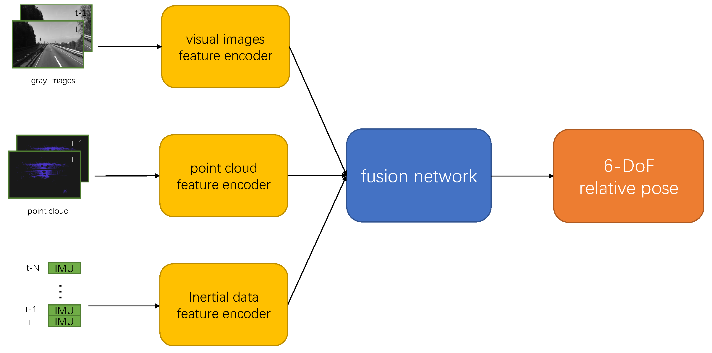
For the stated reasoning, we introduce an end-to-end visual-lidar-inertia odometry framework. Initially, we employ CNN to encode grayscale images and 3D point clouds, and RNN for inertial data. Notably, the 3D point clouds are projected into 2D images to align with CNN. Subsequently, the resulting feature vectors are concatenated and remapped to derive a 6-DoF relative pose. Finally, we train our framework in a supervised manner, utilizing the L2 norm. The main contributions of our work are as follows:
We utilize grayscale images, 3D point clouds, and inertial data as inputs to compensate for the weakness of each sensor, encoding these data by deep neural networks;
We introduce a novel fusion module that reorganizes and remaps feature vectors to adapt to challenging scenes by introducing an attention mechanism and auxiliary vectors;
We evaluate the performance of our framework on the KITTI odometry benchmark. A comparison with several variants demonstrates the effectiveness of our algorithm.
The rest of the paper is structured as follows:
Section 2 introduces related work on the odometry task, categorized as traditional and deep works.
Section 3 provides details about our algorithm.
Section 4 presents the experimental results on the KITTI odometry benchmark. Finally, in
Section 5, we conclude the paper and discuss our future plans.
2. Related Work
In this section, we provide an overview of traditional and deep methods applied to the odometry problem. Given our primary focus on multisensory UGVs, we emphatically discuss deep sensor fusion methods. As illustrated in
Figure 1, odometry methods estimate the relative pose between two scenes using information from various sensors.
2.1. Traditional Odometry
Behley et al. [
5] employed a 2D vertex map and a normal map projected from 3D point cloud to estimate odometry efficiently. While suitable for mapping large outdoor scenes, their algorithm needs to exclude the influence of dynamic objects. Mur-Artal et al. [
6] utilized oriented FAST and rotated BRIEF (ORB) feature from visual images to achieve real-time operation. However, the extraction of ORB features resulted in sparse point clouds in the generated map, and the running speed was limited. Moreover, this approach was sensitive to dynamic objects, leading to tracking loss. In contrast to pre-computed features, Engel et al. [
7] directly employed visual light intensity for motion tracking and can generate a map of dense point clouds. However, this approach had high requirements for scene illumination and demanded that the sensor maintain stable exposure. Zhen et al. [
8] updated inertial and lidar measurements using a Gaussian particle filter. Subsequently, the outputs were fused using an error state Kalman filter to meet the real-time requirements of UAVs. Although it was efficient, this method did not consider the impact of the system state on the measurements, resulting in cumulative errors. Qin et al. [
9] proposed a tightly-coupled visual-inertial system comprising a monocular camera and a low-cost IMU, which achieved highly accurate odometry by fusing pre-integrated IMU measurements and feature observations. As the method used the optical flow method to track and match feature points, the images need to be clear and continuous; otherwise, it will lead to the drift of the predicted trajectory. Shan et al. [
10] introduced a tightly-coupled lidar-inertial odometry framework that incorporated a factor graph to effectively fuse lidar and IMU measurements. The factor graph framework they proposed demonstrated good compatibility. Graeter et al. [
11] combined visual images with the depth information extracted from lidar measurements to estimate ego-motion. This method only used the point clouds in the visual field of the images to provide depth information, and the lidar was not fully utilized. Shan et al. [
12] developed a tightly-coupled lidar-visual-inertial odometry framework based on a factor graph. This framework includes a visual-inertial system and a lidar-inertial system, mitigating the risk of single subsystem failure.
2.2. Deep Odometry
Li et al. [
13] presented a deep convolutional network for odometry estimation. They projected 3D lidar point clouds into 2D images using cylindrical projection and then converted them into normal images to ensure geometric consistency. In contrast, Adis et al. [
14] did not project 3D lidar point clouds but instead utilized mini-PointNet to directly handle point clouds, taking full advantage of point clouds. However, obtaining local point cloud features with PointNet in this method proved challenging, making the analysis of complex scenes difficult. Konda et al. [
15] were the first to apply deep learning to visual odometry. They employed a simple CNN structure to predict direction and velocity from stereo images using the softmax function. But as an early attempt in this field, they had a poor accuracy of prediction. Zhou et al. [
16] proposed an unsupervised framework for learning ego-motion and depth information from video sequences, with view synthesis serving as a supervisory signal. However, they did not explicitly incorporate dynamic objects and occlusion into the constraints, resulting in reduced robustness of the method in scenes that include both. Chen et al. [
17] treated inertial odometry as a sequential learning problem and introduced a deep neural network based on long short-term memory (LSTM) structure to learn location transforms. However, the performance of their method is easily affected by the high bias value of IMU, and the generalization ability of the neural network is not strong.
The combination of multiple sensors can have a complementary effect. Clark et al. [
18] introduced the first end-to-end trainable method for visual-inertial odometry. Their experiments demonstrated that the visual-inertial odometry method based on deep learning is more robust than conventional methods, particularly when there are errors in sensor calibration parameters. However, they simply concatenated features extracted from RGB images and inertial data without deploying a sensor fusion strategy. Han et al. [
19] used a fully connected layer to fuse the outputs of RGB images and inertial data encoder, allowing for the update of additional bias for the IMU. Despite this, drift problems still exist in their method due to the absence of place recognition and relocalization pipelines. Son et al. [
20] employed the softmask-based method to fuse lidar and inertial data, enabling the learning of the weights of each sensor. Their method relied on a multilayer perceptron (MLP), which may not be sufficient to handle challenging situations in the real world. Sun et al. [
21] combined soft mask attention fusion (SMAF) and a transformer for lidar-inertial odometry estimation task, addressing the overfitting problem associated with transformer networks. Moreover, it is able to fuse a mixture of heterogeneous sensor data, such as lidar and IMU. However, their fusion module suffers from high redundancy and is not beneficial for easy training and real-world applications. Aydemir et al. [
22] fused the lidar and visual data using Bayesian inference to enhance depth maps, resulting in improved scale recovery. This method is a hybrid framework, and the sub-neural network needs to be trained separately, which can be cumbersome. Li et al. [
23] adopted a siamese network architecture with input from both flipped depth and RGB images. They introduced a flip consistency loss to facilitate network learning, but it is susceptible to fall into local optima. Song et al. [
24] proposed a feature pyramid network to fuse lidar point clouds and visual images, enhancing odometry accuracy across different levels. However, their method highly relied on photometric consistency; otherwise, errors are amplified through the pyramid structure.
3. Method
In this section, we describe the details of our odometry framework. Given two frames, P and Q, corresponding to time steps t and t + 1, our objective is to estimate the 6-DoF relative pose (translation on the x, y, and z axes, angle of roll, pitch, and yaw) between them. Our system comprises feature networks and a fusion network. The feature networks encode the features from visual images, 3D point clouds, and inertial data. The fusion network combines these feature vectors to calculate the transformation estimation between the two frames. The pipeline of our framework is illustrated in
Figure 2.
3.1. Data Encoding
3.1.1. Visual Images Feature Encoding
The inputs to the visual images feature encoder are two consecutive grayscale images. The encoder starts with two 5 * 5 convolutional layers, followed by two 3 * 3 convolutional layers. These layers are responsible for extracting features from the grayscale images. Each of the four convolutional layers is followed by a max-pooling layer and a rectified linear unit to reduce the size of images and introduce nonlinearity to the network. The remaining structure is a 1 * 1 convolutional layer, which is used to adjust the dimension of the feature vector. The convolutional layers are detailed in
Table 1.
3.1.2. Point Cloud Feature Encoding
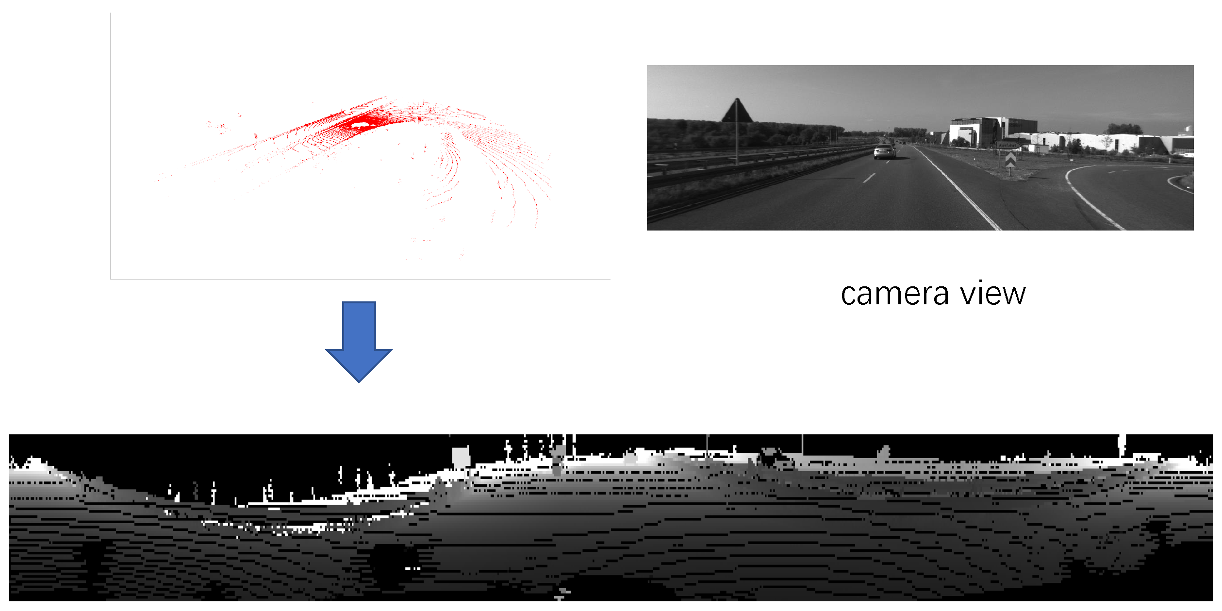
We project the 3D point clouds into a 2D image. Since a point can be represented as a 3D coordinate
, its 2D coordinate
should be
where
H is the height of the 2D image,
W is the width of 2D image,
is the azimuth angle,
is the elevation angle,
and
are the vertical and horizontal view angle of the lidar sensor, and
and
are the mean of the top and bottom limitation of the view angle. The position
of the 2D image is filled with the range value
. If several points have the same 2D coordinate, we keep the point with the smallest range value. The effect of converting a point cloud into a depth map is shown in
Figure 3.
The point cloud feature encoder has a similar structure to the visual images feature encoder. The inputs of the encoder are two range images projected by two consecutive frames of point clouds. Note that we abandon the max-pooling layer in this encoder since contrast experiments indicate that it decreases the estimation accuracy. Without max-pooling layers, we adjust the kernel size and stride to reduce the size of the images. The convolutional layers are detailed in
Table 2.
3.1.3. Inertial Data Feature Encoding
Inertial data are typically available at higher frequency (100 Hz) compared to images (10 Hz). To align the inertial data with visual images and point clouds, we use spherical linear interpolation. We use quaternions to represent inertial data. Given two quaternions
and
, corresponding to time steps
and
, the quaternion
, corresponding to time step
t (
), is expressed as follows:
where · denotes dot product.
The input of the inertial data feature encoder is composed of two consecutive inertial measurements. Due to the kinematic connection between inertial data and time, we choose RNN as the encoder. The RNN in our setup is a two-layer Bi-directional LSTM with 128 hidden states. The choice of Bi-directional LSTM is motivated by its ability to extract features from both preceding and succeeding inertial data.
3.2. Fusion Module
Features extracted from different sensors are complementary but not equally important in certain scenes. For instance, when a multitude of dynamic objects populate the scene, the contribution of visual and LiDAR features to pose estimation should be diminished. Inspired by the attention mechanism [
25,
26], we introduce a novel method for feature vector fusion. Rather than employing a weight function, we utilize a fully connected network to reorganize feature vectors, thereby achieving better fine-grained attention. So, we put feature vectors into the function:
where
is the visual images feature vector,
is the point cloud feature vector,
is the inertial data feature vector, FC is the fully connected network, and ⊕ denotes concatenating two feature vectors together.
Then we remap the feature vector for different targets to further improve the pose estimation accuracy. Given that the output is a 6-dimensional vector, the reorganized feature vector is concatenated with six independent vectors respectively. Each of independent vectors is deterministically parameterized by the network and updated using gradient descent. Thus, these recombined vectors are passed through six separate fully connected networks to obtain the final output. The remapping function can be described as follows:
where
is the reorganized feature vector calculated by function
8 and
is the independent vector (
). The detail of the fusion module is shown in
Figure 4.
3.3. Loss Function
The output of our network is a 6-DoF relative pose
v:
where
p is a 3D translation vector and
r is a 3D Euler rotation vector. Our loss function of the network is defined as follows:
where
is ground truth of translation vector,
is ground truth of Euler rotation vector,
means L2 norm, and
is a scale factor to balance the error of translation and rotation. In our experiment,
is chosen as 100.
4. Experiment
In this section, we introduce the details of training and experiment. We compare our method with several representative works on the odometry task. We also compare our method with its variants.
4.1. Dataset and Evaluation Metrics
We choose the KITTI odometry benchmark for our experiment, which comprises 22 sequences containing grayscale images, color images, and Velodyne laser data. Among these sequences, 10 (00, 01, 02, 03, 04, 05, 06, 07, 08, 09, 10) provide ground truth pose data. Additionally, corresponding inertial data are available in the KITTI raw data for all sequences except Sequence 03. For our training, we utilized Sequence 00, 01, 02, 04, 05, 06, 07, 08, and for testing, we used Sequence 09 and 10.
Table 3 shows the details of the KITTI odometry benchmark.
To evaluate the pose estimation results, we follow the official criteria outlined in the KITTI benchmark [
27]. This metric is calculated by averaging the root mean square errors of the translation and rotation for the involved sequences of lengths (100, 200, 300, 400, 500, 600, 700, 800) meters. Formally, the error metrics are defined as follows:
where
F is the set of frames
,
i and
j represent the subscript of two frames separated by a fixed distance, length(
) represents the fixed distance, Trans() and Rot() represent figuring out the rotation and translation respectively, ⊖ denotes calculating the relative pose transformation between two frames, and
and
p represent the estimated and true values of pose. The evaluation metrics of the KITTI dataset incorporates the length of the trajectory into the metric, which gives the final error a clear physical meaning.
4.2. Baselines
Several traditional and deep odometry works are chosen as baselines, including DeepVO [
28], DeepLO [
29], Au et al. [
30], Chen et al. [
31], EMA-VIO [
32], DeepLIO [
33] and LOAM [
34]. These deep learning methods share similar encoder structures with our method, comprising simple CNN and RNN. DeepVO [
28] proposed a deep recurrent convolutional neural network to estimate pose changes from a sequence of RGB images. DeepLO [
29] projected point clouds into a vector map and a normal map, extracting features to train for relative pose. Au et al. [
30] employed lidar data projection onto the image plane to generate depth images. They used three depth images from different angles along with one RGB image as input for their CNN. Chen et al. [
31] proposed a selective sensor fusion module, akin to attention mechanisms, to weight different features. EMA-VIO [
32] introduced an external memory mechanism based on a transformer when fusing visual and inertial data, showing good performance in accuracy and robustness. DeepLIO [
33] used the soft mask-based method, which relied on MLP to learn the weights of lidar and inertial data. LOAM [
34] extracted edge points and planar points from two scans of lidar and figured out the ego-motion using the Levenberg–Marquardt method.
DeepVO [
28] used Sequence 00, 02, 08, 09 for training and Sequence 03, 04, 05, 06, 07, 10 for testing. DeepLO [
29] and Au et al. [
30] used Sequence 00, 01, 02, 03, 04, 05, 06, 07, 08 for training and Sequence 09, 10 for testing. Chen et al. [
31] used Sequence 00, 01, 02, 03, 04, 06, 08, 09 for training and Sequence 05, 07, 10 for testing. EMA-VIO [
32] and DeepLIO [
33] used Sequence 00, 01, 02, 04, 05, 06, 07, 08 for training and Sequence 09, 10 for testing. DeepVO [
28], Chen et al. [
31], EMA-VIO [
32], and DeepLIO [
33] trained in a supervised manner. DeepLO [
29] and Au et al. [
30] trained in an unsupervised manner. LOAM [
34] is a traditional work that has good performance on the KITTI odometry benchmark.
4.3. Implementation Details
We implement our method based on the PyTorch framework and train our network using a single NVIDIA RTX 2080Ti. Adam optimizer is used in our training with and . The initial learning rate is 10-4 and controlled by a step scheduler with a patience of 5 and factor of 0.5. Batch size was set to 5. Our model is trained for 500 epochs. Note that we do not use normalization layers in our architecture since our experiments show that adding these layers decreases the accuracy of prediction.
4.4. Result of Comparison
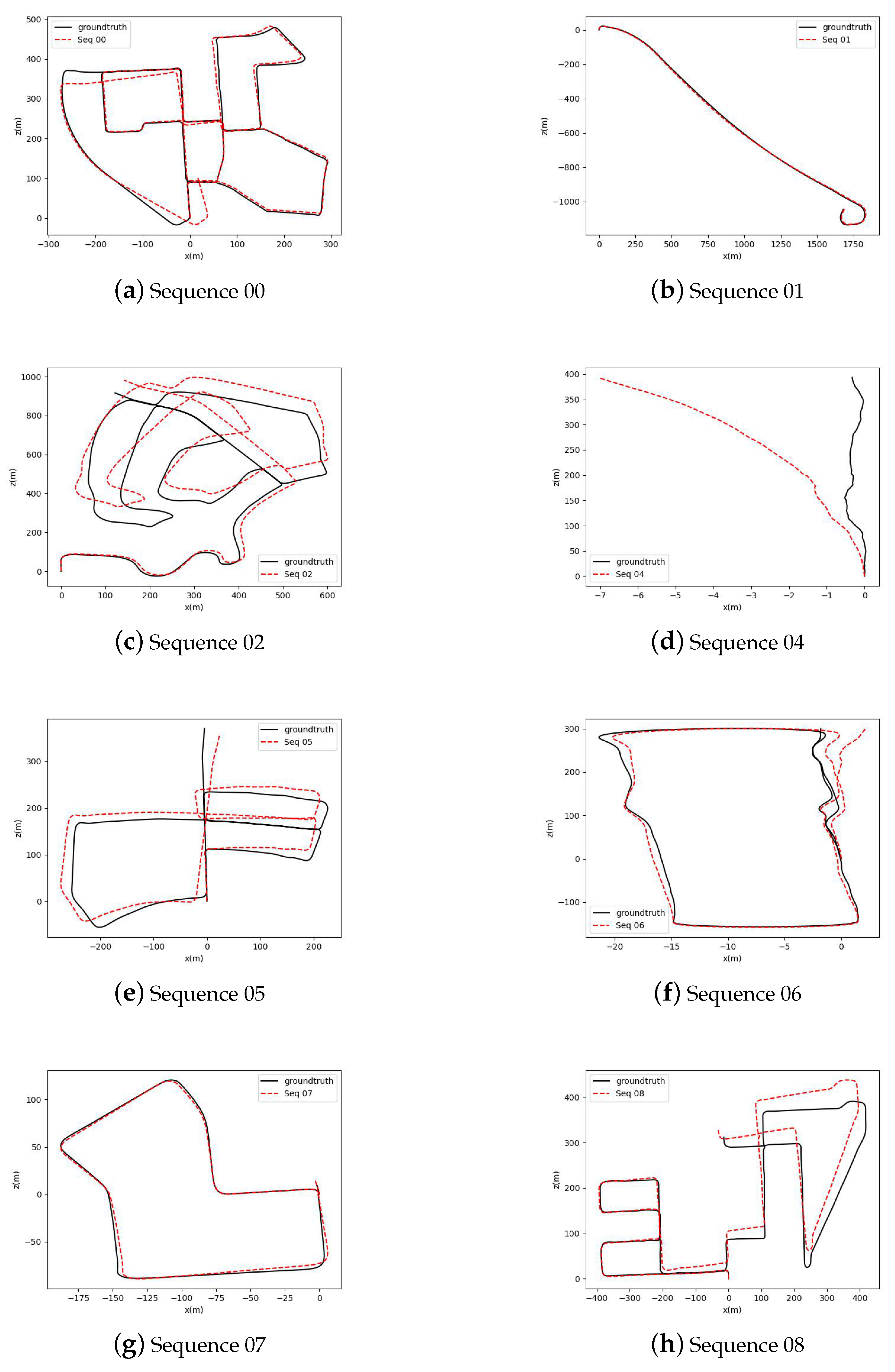
Figure 5 shows the result of our training on the training set. We can see that the motion trails predicted by our method fit the ground truth. As shown in
Table 4, we conducted a comparative analysis of our method against baselines on the odometry task. Our method exhibits superior performance compared to most of baselines, especially when compared to DeepLO [
29] and Au et al. [
30] on the training set (Sequence 00, 01, 02, 04, 05, 06, 07, 08). Notably, sequence 01 includes more dynamic objects than other sequences since it was recorded on a busy highway. Consequently, DeepLO [
29], DeepLIO [
33] and LOAM [
34] display higher translation errors in Sequence 01 due to interference from dynamic objects. In contrast, our method demonstrates remarkable robustness in Sequence 01, attributed to the adoption of multisensory inputs, particularly inertial data, proving to be immune to dynamic objects’ interference. On the testing sets, our method outperforms both DeepVO [
28] and DeepLO [
29], both of which rely on a single sensor. While our method excels in translational accuracy compared to multisensory methods, it does show higher rotational errors in Sequence 10. It is worth noting that both Au et al. [
30] and Chen et al. [
31] utilized RGB images as inputs, which contain more features but require more memory during training. Additionally, some inertial data are missing for certain timesteps in the KITTI raw data, resulting in errors during normalized interpolation of inertial data. DeepLIO [
33] performs better than other methods in rotational accuracy, proving that the combination of point clouds and inertial data can extract more accurate information to predict rotation. Although there is still a performance gap between our method and LOAM [
34], it is important to highlight that our method does not require precise calibration matrices.
4.5. Ablation Studies
We conduct several experiments to investigate the effectiveness of our feature fusion network by generating variants of our framework. For this purpose, we test the following variants: (1) VLIO1: this framework concatenates feature vectors directly; (2) VLIO2: this framework uses the function
8 to fuse feature vectors but do not concatenate the reorganized feature vector with six independent vectors respectively; (3) VLIO3: the full framework. To prove the necessity of feature fusion, we also test three other variants: (1) VLO: this framework takes grayscale images and 3D point clouds as input; (2) VIO: this framework takes grayscale images and inertial data as input; (3) LIO: this framework takes 3D point clouds and inertial data as input. The above three frameworks use full fusion network.
Table 5 shows the relative pose estimations. When comparing VLIO with VLO, VIO, and LIO, we observe that the fusion of different sensors enhances the estimation performance. When compared to VLIO1, the performance of VLIO2 validates the effectiveness of our fusion network. Similarly, when compared to VLIO2, the performance of VLIO3 validates the effectiveness of the remapping.
Figure 6 shows the motion trails of Sequence 09 and Sequence 10 in the x-z plane. It is apparent that the motion trail generated by VLIO3 closely aligns with the ground truth in comparison to the trails of other variants. Additionally,
Figure 7 presents the translational and rotational errors of Sequence 09 and Sequence 10, averaged over sub-sequences with a length of (100, 200, …, 800) meters and different speeds of measurement platform. We can see more clearly that our method’s performance is superior to other variants. In addition, our method has a flatter curve and is insensitive to the change of speed, indicating that our proposed fusion module effectively enhances the robustness of the system.
5. Conclusions
In this paper, we present a novel attention-based odometry framework for multisensory UGV. Our method fully leverages the complementary properties of monocular cameras, lidar, and IMU by taking grayscale images, 3D point clouds, and inertial data as inputs. To enhance the robustness and prediction accuracy of the system, we employ neural networks as encoders and carefully tune the network parameters to optimize overall performance. CNN excels at processing image information, enabling us to extract feature vectors from grayscale and depth images. Notably, the depth images are generated from 3D point clouds, simplifying point cloud data processing for neural networks. We utilize RNN to extract feature vectors from inertial data, modeling the temporal correlation within consecutive inertial data sequences. After extracting these three feature vectors, we introduce a novel feature fusion method inspired by the attention mechanism. Initially, we employ a fully connected network to adjust the weights of the three feature vectors, enhancing the granularity of the resulting features. Subsequently, we remap the reorganized feature vector into six different outputs, thereby achieving greater accuracy. For our experiments, we select the KITTI dataset, which contains data from various sensors and diverse environmental conditions. The results of our experiments demonstrate that our method outperforms other deep learning methods with similar encoder structures. This comparison emphasizes that multisensory odometry offers higher accuracy and robustness in challenging scenarios compared to single-sensor odometry. Ablation studies further confirm that our proposed feature fusion module significantly enhances the performance of deep learning methods. Nevertheless, we have employed a simple CNN structure as an encoder and fine-tuned neural network parameters.
In this paper, our method has been exclusively tested on the KITTI dataset, encompassing urban, highway, and country scenes. However, it does not cover diverse environments like indoor or wooded areas. To adapt our method for alternative datasets, it is crucial to synchronize timestamps across different sensors. Additionally, each sensor’s data undergo preprocessing to attain a format suitable for CNN and RNN processing.
Despite the promising results, our method faces several challenges. The neural network structure proposed exhibits limited generalization ability, performing less optimally on testing sets compared to training sets. To address this, we plan to explore more advanced encoders and broaden training to encompass diverse datasets, thereby enhancing generalization capabilities. Furthermore, we observed an accumulation of errors over time, resulting in a significant final error between the predicted trails and the ground truth. Introducing closed-loop optimization is imperative to continuously correct deviations. Lastly, our method currently relies on ground truth, limiting its applicability in scenarios where ground truth is unavailable. Consequently, we aim to incorporate unsupervised learning to mitigate dependence on ground truth.


