Using UAVs and Machine Learning for Nothofagus alessandrii Species Identification in Mediterranean Forests

Abstract

This study explores the use of unmanned aerial vehicles (UAVs) and machine learning algorithms for the identification of Nothofagus alessandrii (ruil) species in the Mediterranean forests of Chile. The endangered nature of this species, coupled with habitat loss and environmental stressors, necessitates efficient monitoring and conservation efforts. UAVs equipped with high-resolution sensors capture orthophotos, enabling the development of classification models using supervised machine learning techniques. Three classification algorithms—Random Forest (RF), Support Vector Machine (SVM), and Maximum Likelihood (ML)—are evaluated, both at the Pixel- and Object-Based levels, across three study areas. The results reveal that RF consistently demonstrates strong classification performance, followed by SVM and ML. The choice of algorithm and training approach significantly impacts the outcomes, highlighting the importance of tailored selection based on project requirements. These findings contribute to enhancing species identification accuracy in remote sensing applications, supporting biodiversity conservation and ecological research efforts.

1. Introduction

Nothofagus alessandrii Espinosa (ruil) is an endangered species that is endemic to the Mediterranean area of Chile. Since the beginning of the 20th century, its habitat has been reduced because of the expansion of the agricultural frontier with wheat crops and, since the 1970s, the substitution of forest plantations with non-native species. The current area of N. alessandrii forest is approximately 314 ha [1]. In addition, these forests have recently been affected by forest fires of great magnitude and intensity, and persistent drought conditions [2].

The use of unmanned aerial vehicles (UAVs) has allowed for its application to various activities, including those dedicated to forest resources. Recently, data sets based on unmanned aerial vehicles (UAVs) have been found to be quite useful for identification of forest features due to their relatively high spatial resolution [3]. Numerous studies have demonstrated the potential of UAVs for sustainable forest planning, volume estimation, pest infestation detection, tree counting, forest density determination, and canopy height assessment [4]. UAVs are being used in several countries to control natural vegetation based on information in the optical and infrared spectra to spatial resolutions of 5 cm [5]. The imagery acquired with a UAV reaches sub-decimeter or even centimeter resolution, often referred to as hyperspatial imagery, at flying height of 50 m and 18 mm focal length [6]. UAV imagery can be captured on demand, enabling frequent imagery acquisition and efficient monitoring, known as hypertemporal imagery [6]. UAVs are also being used to monitor the state of drought in forests and natural areas to prevent fires [7]. Koh and Wich [8] ran an application to map forest areas, where a UAV was used to map tropical forests in Indonesia. The authors suggested that the use of UAV remote sensing could save time, cost, and manpower for these purposes. The number of trees or the composition of stands are important parameters in sustainable forest planning and management [9]. Fast and accurate determination of canopy cover can be achieved using UAVs [10], leading to decisions that improve optimal stand quality and productivity. For example, Hassaan et al. [11] used a UAV to count trees in urban areas and identified trees with the accuracy of 72%. Likewise, Wallace et al. [12] successfully detected the number of trees using LiDAR (Light Detection And Ranging) sensors mounted on a UAV.

Moreover, UAVs have been combined with Geographic Information Systems (GIS) to gather data on the Earth’s surface and atmosphere. GIS data provide spatial information on Earth’s features, along with their attributes and spatial relationships, and the integration of machine learning techniques in GIS analysis has shown promise in enhancing the speed, accuracy, automation, and repeatability of data processing [13].

Machine learning, as a subfield of Artificial Intelligence (AI), holds significant potential for addressing complex spatial problems within Geographic Information Sciences [14]. Machine learning algorithms allow systems to learn from data, generating data-based predictions by identifying patterns in historical data and applying them for future predictions [15].

Supervised learning, a form of machine learning, involves training models on labeled data and testing them on unlabeled data, making it well suited for classification problems. To address the need for robust species identification, we evaluate three classification algorithms in this research: Maximum Likelihood, Random Forest, and Support Vector Machine (SVM).

Random Forest, as proposed by Breiman [16], is a powerful ensemble learning technique that has gained popularity due to its versatility and minimal parameter-tuning requirements, making it suitable for a wide range of prediction problems. RF leverages the collective decision making of multiple decision trees, each trained on a random subset of predictor variables. This approach yields highly accurate results and has demonstrated exceptional performance in numerous ecological and remote sensing applications.

Support Vector Machine, on the other hand, is a set of machine learning algorithms renowned for its effectiveness in data analysis [17]. SVM offers advantages such as fine-grained control over error frequencies, decision rule transparency, and computational efficiency [18]. SVM’s ability to achieve remarkable results with limited training samples makes it particularly relevant for species identification from orthophotos [19].

Maximum Likelihood, often referred to as ML, is a classical classification method that estimates membership probabilities for each class and assigns a pixel to the class with the highest probability [20]. ML is grounded in two fundamental principles: the assumption of normal distribution within each class in a multidimensional feature space and the application of Bayes’ theorem for decision making [21].

To assess the classification accuracy of these three algorithms (RF, SVM, and ML), we conducted an accuracy assessment. This step involves comparing predicted classification results with reference data and provides valuable insights into the reliability of the results [22]. The metrics we employ include the Kappa coefficient, user accuracy, producer accuracy, and F1 score, which collectively offer a comprehensive evaluation of the classification performance. These metrics illuminate the strengths and limitations of each classification method, helping to determine the most suitable approach for species identification in orthophotos.

Our selection of these algorithms is based on their popularity in solving classification problems, their ability to enhance weaker methods, and their widespread application in ecology, including neighborhood models [23,24,25].

In contrast to the broad utilization of UAVs in our country, their application in forestry research, particularly in information-processing studies with machine learning tools, remains limited. Therefore, this study aims to evaluate the effectiveness of a UAV-based approach combined with machine learning algorithms in accurately identifying and classifying the distribution of Nothofagus alessandrii.

Overall, this study contributes to the growing body of research aimed at enhancing the accuracy and reliability of species identification in remote sensing applications, with the potential to support biodiversity conservation and ecological research efforts.

2. Materials and Methods

2.1. Study Area

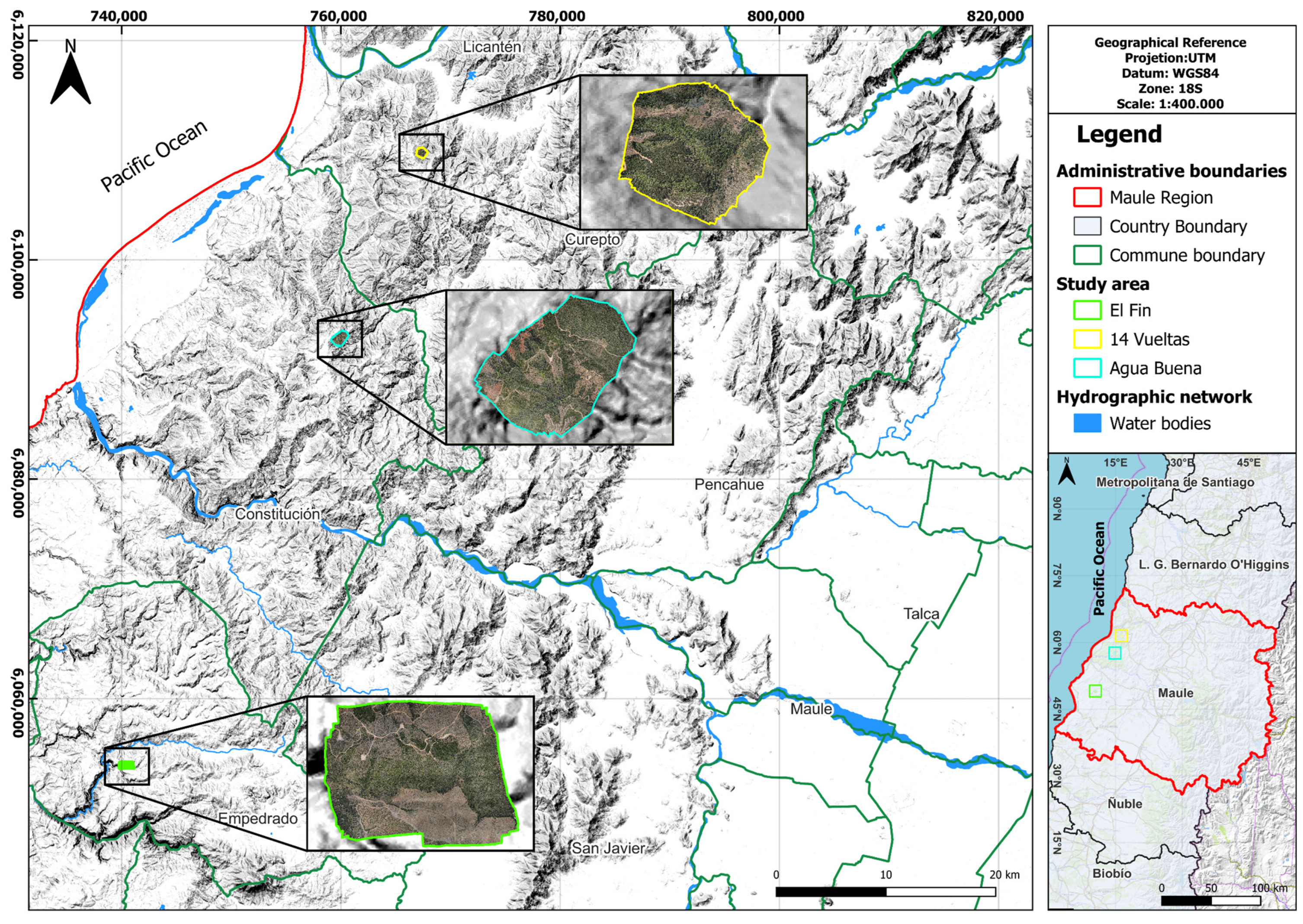
The current area of N. alessandrii forest is just over 314 ha, with forest stands occurring in four communities in 15 locations, for a total of 305 stands with an average stand size of 1.03 ha [1]. Out of these 15 locations, we selected 3 (Figure 1) due to their significance in hosting N. alessandrii populations and their unaltered state following the 2017 wildfires [26]. The variations in their sizes and altitudes offer a diverse set of data to analyze and draw conclusions about the vegetation distribution and classification methods employed. According to the study conducted by Santelices et al. (2012) [1], the surface area of N. alessandrii is 3.6 hectares, 1.5 hectares, and 10.2 hectares, respectively, in “14 Vueltas”, “Agua Buena”, and “El Fin”. The polygons generated in that study serve as the basis for the visual identification of the species in the generated orthophotos.

The study area “14 Vueltas” is located in the commune of Curepto (−72.066104°, −35.119434°) at an approximate altitude of 196 m (above sea level) with an area of 69.95 ha, while “Agua Buena” is located in the commune of Constitución (−72.142403°, −35.273924°) at an altitude of 333 m (above sea level) and an area of 141,33 ha; finally, “El Fin” is located in the commune of Empedrado (−72.344827°, −35.629865°) at an altitude of 341 m (above sea level) with an area of 145.69 ha. The mean annual temperature is equal to 14.2 °C, and the mean annual rainfall is 845 mm [9].

2.2. Data Acquisition

The images of the study areas “14 Vueltas”, “Agua Buena”, and “El Fin” were acquired on 3 October, 14 November, and 25 November, respectively, using a Dji Matrice 300 RTK and a Dji Zenmuse P1 sensor (SZ DJI Technology Co., Shenzhen, China). The sensor is highly sensitive, has 45 MP and flexible vision with 35 mm lens (FOV 63.5°). The images were acquired under ideal weather conditions, with low cloud cover and close to noon, in order to avoid shady areas. The flight height was 120 m above ground level. The images were registered in continuous mode at 2 s intervals and speed of 3.5 m s⁻¹, resulting in side and forward overlaps equal to 90% and 70%, respectively. On the other hand, it was not necessary to use Ground Control Points (GCPs) due to the inclusion of GNSS-IMU technology within the sensor. We used Agisoft Metashape software (Agisoft LLC., St. Petersburg, Russia; version 1.7.3) for photogrammetric processing. The classification of Nothofagus alessandrii was facilitated by the distinctive light-green hue exhibited by this species compared with its companion species, including Nothofagus glauca (Phil.) Krasser, Crytocarya alba (Molina) Looser, Lithraea caustica (Molina) Hook. et Arn., Peumus boldus Molina, Azara dentata Ruiz and Pav., Luma apiculata (DC.) Burret, Aextoxicon punctatum Ruiz et Pav, and Lomatia hirsuta (Lam.) Diels ex J.F. macbr. The conspicuous differences in foliage coloration and spectral characteristics between N. alessandrii and these companion species allowed for straightforward visual identification. In addition, since the flights were conducted within an interval of less than two months, it is unlikely that phenological and seasonal variations had a significant impact on the classification results. The supervised classification and accuracy process was performed with Arcgis Pro V2.8 (ESRI, Redlands, CA, USA).

2.3. Image Classification

Figure 2 depicts the workflow of this study, illustrating the execution of each stage.

Following the completion of the flights and the acquisition of orthophotomosaics for each study area, the process proceeded with the classification type. Training data for the classification process were collected in two manners: “Pixel Based” and “Object Based.” For the “Pixel Based” approach, training samples were collected at the pixel level. A total of 405 training samples were selected for each target class, which included N. alessandrii, other species, and bare ground, across the three study areas, resulting in a combined total of 1215 polygons per site. The training sample sizes are summarized in

Table 1. Training sample sizes for land cover classes in different study areas.

Study Area	Class	Training Sample Size
		Minimum		Maximum
		Area (m2)	No. Pixel	Area (m2)	No. Pixel
14 Vueltas	N. alessandrii	0.003	2	3.5	2612
	Other species	0.04	29	1.47	7825
	Bare ground	0.038	28	48.41	36,190
Agua Buena	N. alessandrii	0.001	2	5.9	1491
	Other species	0.002	5	10.01	2541
	Bare ground	0.049	12	0.049	18,442
El Fin	N. alessandrii	0.005	2	0.525	258
	Other species	0.019	9	9.87	4855
	Bare ground	0.49	21	28.83	14,189

.

In the “Object Based” approach, object segmentation was performed to create training samples based on image objects rather than individual pixels. Objects were defined using the Segment Mean Shift function in ArcGis, and training samples were extracted from these objects. A total of 405 training objects were created for each class and each study area. We used Random Forest, Support Vector Machine, and Maximum Likelihood methods for supervised image classification.

RF requires two parameters [27]: (1) mtry, the number of predictor variables that partition the data at each node; (2) ntree, the total number of trees that are grown in the model run. In the present study, 500 trees in ntree were used for all classification methods. In SVM, a maximum number of samples per class equal to 500 was used [28,29].

2.4. Accuracy Assessment

Once individual class detection is obtained, it is important to determine the accuracy assessment for each of the classification methods. Model accuracy assessment is defined in terms of forecast error or difference between observed and predicted values [22]. To ensure a genuine accuracy assessment, it is essential to have a reference data set with a high level of precision [30]. In this study, a confusion matrix was constructed using 500 randomly selected validation points, enabling the determination of the following accuracy metrics.

2.4.1. C. Kappa

The Kappa coefficient, a widely accepted metric in classification accuracy assessment [31], is easily calculated from the confusion matrix. The Kappa statistic is considered highly reliable for assessing classification accuracy, as it considers all data points in the confusion matrix, not just the diagonal elements [32]. The Kappa statistic yields a value between 0 and 1, where 0 indicates no agreement beyond chance and 1 signifies perfect agreement [33].

2.4.2. User Accuracy

User accuracy (1) is calculated as the ratio of correctly classified pixels within a category to the total number of pixels classified within that category (Maxwell and Warner 2020).

$$\mathrm{User}’\mathrm{s} \mathrm{Accuracy} (\mathrm{UA})=\frac{\mathrm{N}\mathrm{u}\mathrm{m}\mathrm{b}\mathrm{e}\mathrm{r} \mathrm{o}\mathrm{f} \mathrm{C}\mathrm{o}\mathrm{r}\mathrm{r}\mathrm{e}\mathrm{c}\mathrm{t}\mathrm{l}\mathrm{y} \mathrm{C}\mathrm{l}\mathrm{a}\mathrm{s}\mathrm{s}\mathrm{i}\mathrm{f}\mathrm{i}\mathrm{e}\mathrm{d} \mathrm{S}\mathrm{a}\mathrm{m}\mathrm{p}\mathrm{l}\mathrm{e}\mathrm{s} \mathrm{i}\mathrm{n} \mathrm{C}\mathrm{a}\mathrm{t}\mathrm{e}\mathrm{g}\mathrm{o}\mathrm{r}\mathrm{y}}{\mathrm{N}\mathrm{u}\mathrm{m}\mathrm{b}\mathrm{e}\mathrm{r} \mathrm{o}\mathrm{f} \mathrm{S}\mathrm{a}\mathrm{m}\mathrm{p}\mathrm{l}\mathrm{e}\mathrm{s} \mathrm{C}\mathrm{l}\mathrm{a}\mathrm{s}\mathrm{s}\mathrm{i}\mathrm{f}\mathrm{i}\mathrm{e}\mathrm{d} \mathrm{t}\mathrm{o} \mathrm{t}\mathrm{h}\mathrm{a}\mathrm{t} \mathrm{C}\mathrm{a}\mathrm{t}\mathrm{e}\mathrm{g}\mathrm{o}\mathrm{r}\mathrm{y}},$$

(1)

where UA represents the probability measure indicating the likelihood that a sampled pixel belongs to the class as per the reference data [34].

2.4.3. Producer Accuracy

Producer accuracy (2) is a reference-based precision metric that quantifies the percentage of correct predictions for a given class [35]. It assesses errors of omission and the classification performance of different land cover types [36].

Producer accuracy is computed by dividing the number of correctly classified pixels of a specific class by the total number of reference points for that class [32,37].

$$\mathrm{Producer}’\mathrm{s} \mathrm{Accuracy} (\mathrm{PA})=\frac{\mathrm{N}\mathrm{u}\mathrm{m}\mathrm{b}\mathrm{e}\mathrm{r} \mathrm{o}\mathrm{f} \mathrm{C}\mathrm{o}\mathrm{r}\mathrm{r}\mathrm{e}\mathrm{c}\mathrm{t}\mathrm{l}\mathrm{y} \mathrm{C}\mathrm{l}\mathrm{a}\mathrm{s}\mathrm{s}\mathrm{i}\mathrm{f}\mathrm{i}\mathrm{e}\mathrm{d} \mathrm{S}\mathrm{a}\mathrm{m}\mathrm{p}\mathrm{l}\mathrm{e}\mathrm{s} \mathrm{i}\mathrm{n} \mathrm{C}\mathrm{a}\mathrm{t}\mathrm{e}\mathrm{g}\mathrm{o}\mathrm{r}\mathrm{y}}{\mathrm{N}\mathrm{u}\mathrm{m}\mathrm{b}\mathrm{e}\mathrm{r} \mathrm{o}\mathrm{f} \mathrm{S}\mathrm{a}\mathrm{m}\mathrm{p}\mathrm{l}\mathrm{e}\mathrm{s} \mathrm{f}\mathrm{r}\mathrm{o}\mathrm{m} \mathrm{R}\mathrm{e}\mathrm{f}\mathrm{e}\mathrm{r}\mathrm{e}\mathrm{n}\mathrm{c}\mathrm{e} \mathrm{D}\mathrm{a}\mathrm{t}\mathrm{a} \mathrm{i}\mathrm{n} \mathrm{C}\mathrm{a}\mathrm{t}\mathrm{e}\mathrm{g}\mathrm{o}\mathrm{r}\mathrm{y}},$$

(2)

2.4.4. F1 Score

The F1 score (3), ranging from 0 to 1, with 0 indicating poor performance and 1 indicating perfect classification [38], is used to evaluate the classification results. The F1 score formula incorporates Precision and Recall [37].

$$\mathrm{F}1 \mathrm{S}\mathrm{c}\mathrm{o}\mathrm{r}\mathrm{e}=\frac{2\times \mathrm{P}\mathrm{r}\mathrm{e}\mathrm{c}\mathrm{i}\mathrm{s}\mathrm{i}\mathrm{o}\mathrm{n}\times \mathrm{R}\mathrm{e}\mathrm{c}\mathrm{a}\mathrm{l}\mathrm{l}}{\mathrm{P}\mathrm{r}\mathrm{e}\mathrm{c}\mathrm{i}\mathrm{s}\mathrm{i}\mathrm{o}\mathrm{n}+\mathrm{R}\mathrm{e}\mathrm{c}\mathrm{a}\mathrm{l}\mathrm{l}}$$

(3)

where Precision represents the ratio of correctly classified positive examples to the total examples labeled as positive by the system, while Recall is the ratio of correctly classified positive examples to the total positive examples in the data set [39].

3. Results

3.1. Supervised Classification

The results of our study produced six maps for each study area, providing valuable spatial information on pixel locations for each category using both Object-Based and Pixel-Based supervised classification methods. In

Table 2. Surface area (ha) for each class (N. alessandrii, other species, and bare soil), algorithm type (Random Forests (RF), Support Vector Machine (SVM), and Maximum Likelihood (ML)), and training approach (Object-Based or Pixel-Based).

Study Area	Class	RF		SVM		ML
		Object	Pixel	Object	Pixel	Object	Pixel
14 Vueltas	N. alessandrii	2.05	2.88	2.60	1.86	2.43	1.79
	Other species	52.58	52.40	56.11	53.33	43.50	50.36
	Bare ground	15.26	14.62	11.18	14.71	23.96	17.75
Agua Buena	N. alessandrii	7.53	11.01	10.39	13.00	9.32	9.78
	Other species	104.02	103.07	96.61	98.56	99.58	103.14
	Bare ground	29.92	27.43	34.47	29.96	32.58	28.60
El Fin	N. alessandrii	2.99	4.82	2.94	3.59	4.94	9.78
	Other species	84.53	88.03	83.78	88.47	80.24	103.14
	Bare ground	58.24	52.93	59.03	53.71	60.57	28.60

, we quantify the total area (in hectares) for each class used in the supervised classification.

As can be observed, Table 2 summarizes the surface areas (in hectares) for each class (N. alessandrii, other species, and bare soil) by algorithm type (Random Forests (RF), Support Vector Machine (SVM), and Maximum Likelihood (ML)) and training approach (Object-Based or Pixel-Based approach) across the three study areas. The table provides a clear overview of the variations in surface areas for different classes based on the selected algorithms and training methods.

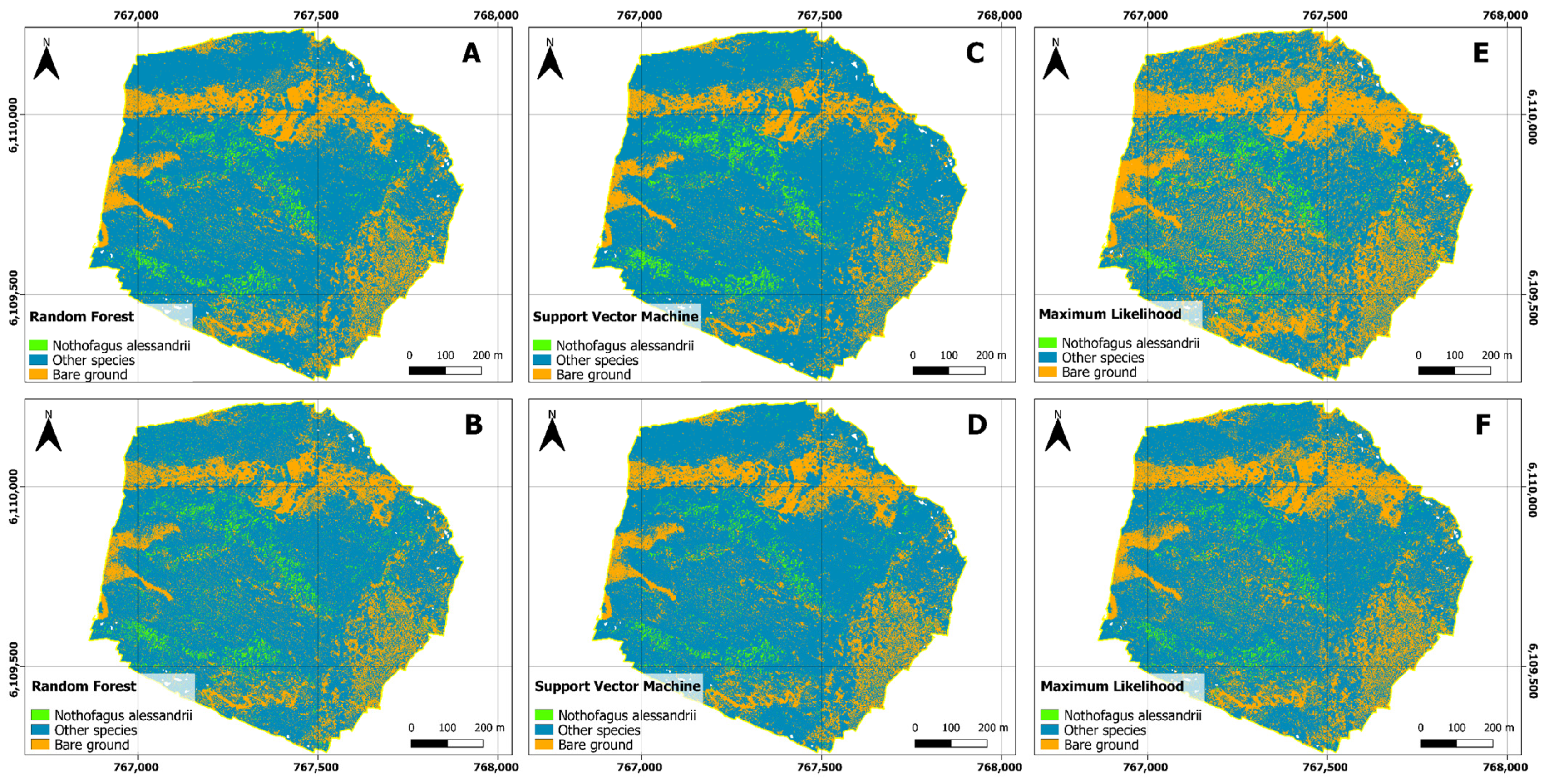
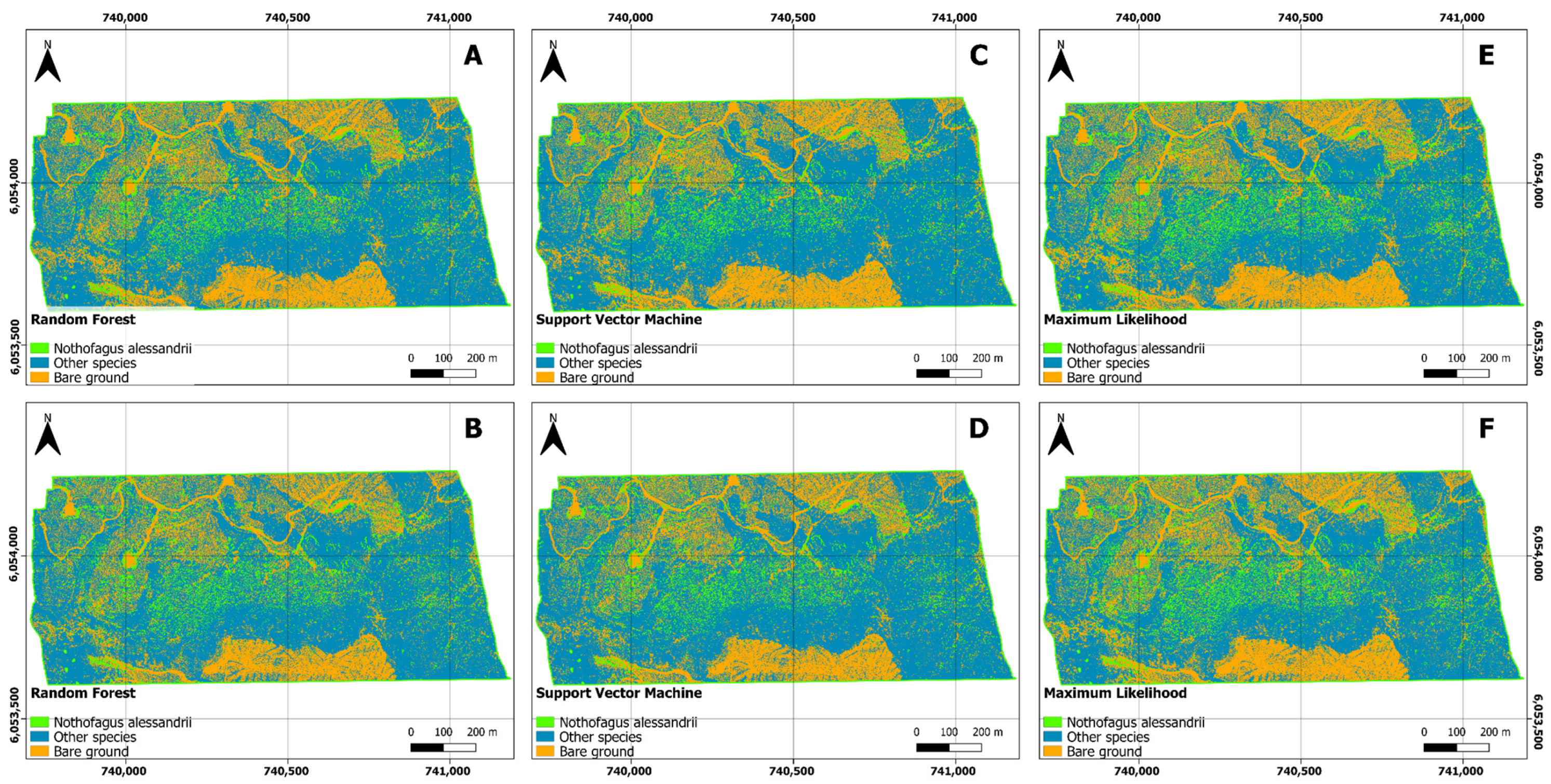
Figure 3, Figure 4 and Figure 5 display the classification results in the three study areas.

3.2. Accuracy Assessment

For the estimation of the accuracy assessment, 500 random points were used for each class for validation in each of the study areas using a confusion matrix. These results allow for a precise evaluation of the results obtained in each class for each classification approach (Object- and Pixel-Based approaches).

Three confusion matrices are presented for three different classification algorithms used in the same study areas and with the same training data sets (Object-Based and Pixel-Based approaches). The algorithms are Random Forest (RF), Support Vector Machine (SVM), and Maximum Likelihood (ML) (

Table 3. Confusion matrix for Random Forest classification by study area and training approach.

Study Area	Class	Object-Based Approach			Pixel-Based Approach
		N. alessandrii	Other Species	Bare Ground	N. alessandrii	Other Species	Bare Ground
14 Vueltas	N. alessandrii	442	25	0	447	52	0
	Other species	58	473	1	50	441	2
	Bare ground	0	2	499	3	7	498
	Total	500	500	500	500	500	500
Agua Buena	N. alessandrii	470	38	0	482	55	0
	Other species	30	455	11	17	434	22
	Bare ground	0	7	489	1	11	478
	Total	500	500	500	500	500	500
El fin	N. alessandrii	489	0	0	497	1	6
	Other species	10	487	12	2	484	11
	Bare ground	1	13	488	1	15	483
	Total	500	500	500	500	500	500

,

Table 4. Confusion matrix for SVM classification by study area and training approach.

Study Area	Class	Object-Based Approach			Pixel-Based Approach
		N. alessandrii	Other Species	Bare Ground	N. alessandrii	Other Species	Bare Ground
14 Vueltas	N. alessandrii	423	25	0	439	47	0
	Other species	77	474	1	61	447	1
	Bare ground	0	1	499	0	6	499
	Total	500	500	500	500	500	500
Agua Buena	N. alessandrii	471	46	1	494	66	0
	Other species	29	442	8	5	422	27
	Bare ground	0	12	491	1	12	473
	Total	500	500	500	500	500	500
El Fin	N. alessandrii	498	0	0	494	1	0
	Other species	2	485	11	5	485	6
	Bare ground	0	15	489	1	14	494
	Total	500	500	500	500	500	500

and

Table 5. Confusion matrix for ML classification by study area and training approach.

Study Area	Class	Object-Based Approach			Pixel-Based Approach
		N. alessandrii	Other Species	Bare Ground	N. alessandrii	Other Species	Bare Ground
14 Vueltas	N. alessandrii	434	32	0	420	40	0
	Other species	66	463	0	80	455	0
	Bare ground	0	5	500	0	5	500
	Total	500	500	500	500	500	500
Agua Buena	N. alessandrii	471	50	0	484	62	0
	Other species	29	439	6	16	427	20
	Bare ground	0	11	494	0	11	480
	Total	500	500	500	500	500	500
El Fin	N. alessandrii	491	1	0	499	6	1
	Other species	9	478	5	1	470	2
	Bare ground	0	21	495	0	24	497
	Total	500	500	500	500	500	500

).

In the RF confusion matrix, based on the percentages of correct predictions in each area, we can observe that overall, the predictions are quite accurate in all cases, with percentages exceeding 88%. These percentages indicate a high rate of success in classification.

Overall, the percentages of correct classification in all study areas are quite high, exceeding 84% in all cases. The “Bare ground” class stands out for having classification rates close to 100%, indicating an exceptional ability of the model to identify this particular class.

In general, the percentages of correct classification in all study areas are quite high, with most categories exceeding 86%. The “Bare ground” class stands out for having a classification rate of 100%, indicating an exceptional ability of the model to identify this particular class. The “Other species” class in the “14 Vueltas” area has the lowest classification rate, but it is still fairly high overall, exceeding 87%.

Below (

Table 6. Random Forest classification performance metrics across study areas and training approaches.

Study Area	Class	Object-Based Approach				Pixel-Based Approach
		Count	User Accuracy	Producer Accuracy	F-Score	Count	User Accuracy	Producer Accuracy	F-Score
14 Vueltas	N. alessandrii	442	0.946	0.884	0.914	447	0.896	0.894	0.895
	Other species	473	0.889	0.946	0.917	441	0.895	0.882	0.888
	Bare ground	499	0.996	0.998	0.997	498	0.980	0.996	0.988
	C. Kappa	k = 0.914				k = 0.886
Agua Buena	N. alessandrii	470	0.925	0.94	0.933	482	0.898	0.964	0.930
	Other species	455	0.917	0.91	0.914	434	0.918	0.868	0.892
	Bare ground	489	0.986	0.978	0.982	478	0.976	0.956	0.966
	C. Kappa	k = 0.914				k = 0.894
El fin	N. alessandrii	489	1.000	0.978	0.989	497	0.986	0.994	0.990
	Other species	487	0.957	0.974	0.965	484	0.974	0.968	0.971
	Bare ground	488	0.972	0.976	0.974	483	0.968	0.966	0.967
	C. Kappa	k = 0.964				k = 0.964

,

Table 7. SVM classification performance metrics across study areas and training approaches.

Study Area	Class	Object-Based Approach				Pixel-Based Approach
		Count	User Accuracy	Producer Accuracy	F-Score	Count	User Accuracy	Producer Accuracy	F-Score
14 Vueltas	N. alessandrii	423	0.944	0.846	0.892	439	0.903	0.878	0.890
	Other species	474	0.859	0.948	0.901	447	0.878	0.894	0.886
	Bare ground	499	0.998	0.998	0.998	499	0.998	0.998	0.993
	C. Kappa	k = 0.896				k = 0.885
Agua Buena	N. alessandrii	471	0.909	0.942	0.925	494	0.882	0.988	0.932
	Other species	442	0.923	0.884	0.903	422	0.930	0.844	0.885
	Bare ground	491	0.976	0.982	0.979	473	0.973	0.946	0.959
	C. Kappa	k = 0.904				k = 0.889
El Fin	N. alessandrii	498	1.000	0.996	0.998	494	0.998	0.988	0.993
	Other species	485	0.974	0.97	0.972	485	0.978	0.97	0.974
	Bare ground	489	0.970	0.978	0.974	494	0.971	0.988	0.979
	C. Kappa	k = 0.972				k = 0.973

and

Table 8. ML classification performance metrics across study areas and training approaches.

Study Area	Class	Object-Based Approach				Pixel-Based Approach
		Count	User Accuracy	Producer Accuracy	F-Score	Count	User Accuracy	Producer Accuracy	F-Score
14 Vueltas	N. alessandrii	434	0.931	0.868	0.899	420	0.913	0.84	0.875
	Other species	463	0.875	0.926	0.900	455	0.850	0.91	0.879
	Bare ground	500	0.990	1	0.995	500	0.990	1	0.995
	C. Kappa	k = 0.897				k = 0.875
Agua Buena	N. alessandrii	471	0.904	0.942	0.923	484	0.886	0.968	0.925
	Other species	439	0.926	0.878	0.901	427	0.922	0.854	0.887
	Bare ground	494	0.978	0.988	0.983	480	0.978	0.96	0.969
	C. Kappa	k = 0.904				k = 0.891
El Fin	N. alessandrii	499	0.986	0.998	0.992	491	0.998	0.982	0.990
	Other species	470	0.994	0.94	0.966	478	0.972	0.956	0.964
	Bare ground	497	0.954	0.994	0.974	495	0.959	0.99	0.974
	C. Kappa	k = 0.966				k = 0.964

) are the results of the Kappa coefficient, user accuracy, producer accuracy, and F1 score for three different classification algorithms used in the same study areas and with the same training data sets (Object-Based and Pixel-Based approaches). The algorithms are Random Forest (RF), Support Vector Machine (SVM), and Maximum Likelihood (ML).

The performance metrics presented in Table 6, Table 7 and Table 8 highlight the robust classification performance achieved across different study areas and training approaches using the Random Forest (RF), Support Vector Machine (SVM), and Machine Learning (ML) algorithms.

4. Discussion

The results of our study demonstrate the effectiveness of three different classification algorithms, namely, Random Forest (RF), Support Vector Machine (SVM), and Maximum Likelihood (ML), in classifying land cover categories across three distinct study areas, including “14 Vueltas”, “Agua Buena”, and “El Fin”. To assess the impact of the training methodology on the classification outcomes, we employed both Object-Based and Pixel-Based training approaches.

RF consistently exhibited high accuracy across all study areas and training approaches, with user accuracy exceeding 88%, producer accuracy over 88%, and F-scores above 0.88. These high values confirm RF’s robustness and versatility in remote sensing applications, as supported by previous research findings [40]. Additionally, the Kappa coefficient values consistently indicated substantial agreement between RF classification results and the actual ground truth, reaffirming its classification accuracy [41].

Similarly, SVM displayed strong classification performance, consistently achieving user accuracy of over 85%, producer accuracy exceeding 84%, and F-scores above 0.88 in most cases [42]. SVM’s ability to identify optimal decision boundaries in complex feature spaces [43] contributed to its effectiveness in classifying land cover categories. In certain instances, SVM outperformed RF by achieving fewer false positives, suggesting a more conservative classification approach.

ML also demonstrated competitive classification performance, with user accuracy consistently above 85%, producer accuracy exceeding 84%, and F-scores above 0.87. Leveraging statistical probability, ML effectively discriminated among land cover classes and performed comparably to SVM in terms of false positives and false negatives.

These findings underscore the significant impact of algorithm and training approach choices on classification outcomes. Notably, the SVM algorithm with Pixel-Based training consistently produced larger surface areas for designated classes across all three study areas, while RF with Object-Based training generally resulted in smaller surface areas. These variations emphasize the need for thoughtful selection of algorithms and training approaches, as they influence both the classification outcome and the delineation of vegetation classes [44].

Our results are consistent with Adugna et al.’s [45]. In their study, the Random Forest (RF) model outperformed Support Vector Machine (SVM) in accurately classifying four distinct land cover types (built-up, forest, herbaceous vegetation, and shrub). Importantly, both algorithms demonstrated nearly identical performance in distinguishing between two classes, namely, bare/sparse vegetation and water bodies, when these classes exhibited distinct spectral characteristics. However, RF showed superior effectiveness when dealing with classes consisting of mixed pixels, including the aforementioned four categories. It is noteworthy to mention SVM’s susceptibility to mixed pixels and inaccurately labeled training samples, which makes it more sensitive to noisy data compared with other classification algorithms [46].

Additionally, our findings align with Sheykhmousa et al.’s [47], who assessed classification accuracy for various study targets. They reported that RF achieved average accuracy of approximately 95.5% in land use and land cover (LULC) classification and about 93.5% in change detection using SVM classification. LULC classification, a common application for both SVM and RF, showed less variability for the RF classifier, indicating higher stability compared with SVM in classification tasks, including crop classification.

Moreover, in a related study by Yang et al. [48], the effectiveness of Random Forest (RF) and Support Vector Machine (SVM) in land cover classification was emphasized. Yang et al. [48] highlighted RF’s robustness and SVM’s ability to handle complex feature spaces, in line with our observations. They also pointed out that compared with Pixel-Based (PB) classification, the Object-Based image analysis (OBIA) method, as Yang et al. [48] indicated, can extract features of each element of remote sensing images, providing certain advantages.

In the context of confusion matrices, all three algorithms (RF, SVM, and ML) demonstrated strong performance in classifying classes across the study areas, with correct classification results, and minimal false positives and false negatives. Nevertheless, variations in the number of false positives and false negatives were observed among the algorithms in specific scenarios. RF appeared to exhibit a more balanced distribution between false positives and false negatives, while SVM and ML tended to have fewer false positives in particular cases.

The choice of classification algorithm (RF, SVM, or ML) should be based on the specific requirements of the study and the weighting of false positives and false negatives in the application. Each algorithm has its advantages and disadvantages, necessitating careful consideration of project objectives and needs.

In order to perceive the quality of the classification, accuracy assessment is inevitable [32]. Carrying out a simple accuracy assessment, using overall accuracy (OA) and Kappa coefficient of agreement (K), with the inclusion of ground truth data, might be the most common and reliable approach to reporting the accuracy of thematic maps. These accuracy measures make classification algorithms comparable when independent training and validation data are incorporated into the classification scheme [47]. In this regard, all three classification algorithms (RF, SVM, and ML) demonstrated robust performance across different study areas and training approaches. Minor differences in performance metrics among the algorithms highlighted their effectiveness in land cover classification tasks. Variations in performance may be attributed to the study areas’ complexity and the distribution of land cover classes. Researchers and practitioners can confidently choose any of these algorithms based on their specific project requirements, as they all offer reliable and consistent classification results.

These findings hold significant implications for land cover classification in remote sensing applications. Researchers and practitioners can confidently select any of the three algorithms (RF, SVM, or ML) based on their specific requirements and available resources, as all three demonstrated strong performance. Additionally, the choice between Object-Based and Pixel-Based training approaches can be made without compromising classification accuracy, offering flexibility in methodological decisions.

However, it is essential to acknowledge some limitations of this study. Firstly, the study areas were limited to three specific regions, and the findings may not generalize to other geographic contexts. Additionally, other factors, such as feature selection and preprocessing methods, could influence classification performance and warrant further investigation [49]. Future research could explore the integration of additional machine learning algorithms and advanced feature engineering techniques to improve classification accuracy [50]. Moreover, assessing the scalability of these methods to larger study areas and their performance under different environmental conditions should be considered.

Furthermore, it is imperative to recognize the critical role of remote sensing in the conservation efforts of endangered species like Nothofagus alessandrii. Given its critically endangered status, the detection and monitoring of Nothofagus alessandrii using remote sensing sensors can provide vital information for its preservation and contribute to the broader understanding of ecosystem conservation.

5. Conclusions

Our findings indicate that RF consistently demonstrated high accuracy and reliability, aligning with its robustness in remote sensing applications. SVM also exhibited strong performance, particularly in complex feature spaces, while ML delivered competitive results. The choice of algorithm and training approach significantly influenced the classification outcomes, underscoring their importance in method selection.

While our results are consistent with prior research, with RF generally outperforming SVM, it is important to note that the selection of the appropriate classification algorithm should be tailored to the specific project requirements, considering the trade-off between false positives and false negatives. These findings offer valuable insights for practitioners and researchers in remote sensing and land cover classification.

To enhance the quality of the conclusions and potentially provide a more comprehensive assessment in the future, further verification and comparison of the results may involve supplementing the algorithms with field data and considering the spatial distribution characteristics of vegetation in the study area. This information could potentially offer insights into the advantages and disadvantages of each method.

References

1. Santelices, R.; Drake, F.; Mena, C.; Ordenes, R.; Navarro-Cerrillo, R.M. Current and potential distribution areas for Nothofagus alessandrii, an endangered tree species from central Chile. Cienc. e Investig. Agrar. 2012, 39, 521–531. [Google Scholar] [CrossRef]
2. Santelices-Moya, R.; Cabrera-Ariza, A.; Silva-Flores, P.; Navarro Cerrillo, R.M. Assessment of a wildfire in the remaining Nothofagus alessandrii forests, an endangered species of Chile, based on satellite Sentinel-2 images. Int. J. Agric. Nat. Resour. 2022, 49, 85–96. [Google Scholar] [CrossRef]
3. Haq, M.A.; Rahaman, G.; Baral, P.; Ghosh, A. Deep Learning Based Supervised Image Classification Using UAV Images for Forest Areas Classification. J. Indian Soc. Remote Sens. 2021, 49, 601–606. [Google Scholar] [CrossRef]
4. Banu, T.; Borlea, G.; Banu, C. The Use of Drones in Forestry. J. Environ. Sci. Eng. B 2016, 5, 557–562. [Google Scholar] [CrossRef]
5. Zarco-Tejada, P.J.; Diaz-Varela, R.; Angileri, V.; Loudjani, P. Tree height quantification using very high resolution imagery acquired from an unmanned aerial vehicle (UAV) and automatic 3D photo-reconstruction methods. Eur. J. Agron. 2014, 55, 89–99. [Google Scholar] [CrossRef]
6. Lucieer, A.; Robinson, S.; Turner, D.; Harwin, S.; Kelcey, J. Using a Micro-Uav for Ultra-High Resolution Multi-Sensor Observations of Antarctic Moss Beds. Int. Arch. Photogramm. Remote Sens. Spat. Inf. Sci. 2012, XXXIX-B1, 429–433. [Google Scholar] [CrossRef]
7. Cruzan, M.B.; Weinstein, B.G.; Grasty, M.R.; Kohrn, B.F.; Hendrickson, E.C.; Arredondo, T.M.; Thompson, P.G. Small unmanned aerial vehicles (micro-UAVs, drones) in plant ecology. Appl. Plant Sci. 2016, 4, 1600041. [Google Scholar] [CrossRef]
8. Koh, L.P.; Wich, S.A. Dawn of Drone Ecology: Low-Cost Autonomous Aerial Vehicles for Conservation. Trop. Conserv. Sci. 2012, 5, 121–132. [Google Scholar] [CrossRef]
9. Cabrera-Ariza, A.M.; Silva-Flores, P.; González-Ortega, M.; Acevedo-Tapia, M.; Cartes-Rodríguez, E.; Palfner, G.; Ramos, P.; Santelices-Moya, R.E. Early Effects of Mycorrhizal Fungal Inoculum and Fertilizer on Morphological and Physiological Variables of Nursery-Grown Nothofagus alessandrii Plants. Plants 2023, 12, 1521. [Google Scholar] [CrossRef]
10. Chianucci, F.; Disperati, L.; Guzzi, D.; Bianchini, D.; Nardino, V.; Lastri, C.; Rindinella, A.; Corona, P. Estimation of canopy attributes in beech forests using true colour digital images from a small fixed-wing UAV. Int. J. Appl. Earth Obs. Geoinf. 2016, 47, 60–68. [Google Scholar] [CrossRef]
11. Hassaan, O.; Nasir, A.K.; Roth, H.; Khan, M.F. Precision Forestry: Trees Counting in Urban Areas Using Visible Imagery Based on an Unmanned Aerial Vehicle. IFAC-PapersOnLine 2016, 49, 16–21. [Google Scholar] [CrossRef]
12. Wallace, L.; Lucieer, A.; Watson, C.S. Evaluating Tree Detection and Segmentation Routines on Very High Resolution UAV LiDAR Data. IEEE Trans. Geosci. Remote Sens. 2014, 52, 7619–7628. [Google Scholar] [CrossRef]
13. Ekeanyanwu, C.; Obisakin, I.; Aduwenye, P.; Dede-Bamfo, N. Merging GIS and Machine Learning Techniques: A Paper Review. J. Geosci. Environ. Prot. 2022, 10, 61–83. [Google Scholar] [CrossRef]
14. Lazar, A.; Shellito, B.A. Comparing machine learning classification schemes—A GIS approach. In Proceedings of the Fourth International Conference on Machine Learning and Applications (ICMLA’05), Los Angeles, CA, USA, 15–17 December 2005; p. 7. [Google Scholar]
15. Cussens, J. Machine Learning. IEEE J. Comput. Control 1996, 7, 164–168. [Google Scholar] [CrossRef]
16. Breiman, L. Random forest. Mach. Learn. 2001, 45, 5–32. [Google Scholar] [CrossRef]
17. Mahdavi, F.; Rajabi, R. Drone Detection Using Convolutional Neural Networks. In Proceedings of the 2020 6th Iranian Conference on Signal Processing and Intelligent Systems (ICSPIS), Mashhad, Iran, 23–24 December 2020; pp. 1–5. [Google Scholar]
18. Siphenini, S. Machine Learning, Classification of 3D UAV-SFM Point Clouds in the University of KwaZulu-Natal (Howard College). Ph.D. Thesis, University of KwaZuku-Natal, Pinetown, South Africa, 2020. [Google Scholar]
19. Tzotsos, A.; Argialas, D. Support Vector Machine Classification for Object-Based Image Analysis. In Object-Based Image Analysis: Spatial Concepts for Knowledge-Driven Remote Sensing Applications; Blaschke, T., Lang, S., Hay, G.J., Eds.; Springer: Berlin/Heidelberg, Germany, 2008; pp. 663–677. [Google Scholar]
20. Frizzelle, B.; Moody, A. Mapping Continuous Distributions of Land Cover: A Comparison of Maximum-Likelihood Estimation and Artificial Neural Networks. Photogramm. Eng. Remote Sens. 2001, 67, 693–705. [Google Scholar]
21. Alimuddin, I.; Irwan. The application of Sentinel 2B satellite imagery using Supervised Image Classification of Maximum Likelihood Algorithm in Landcover Updating of the Mamminasata Metropolitan Area, South Sulawesi. IOP Conf. Ser. Earth Environ. Sci. 2019, 280, 012033. [Google Scholar] [CrossRef]
22. Samantaray, S.; Sahoo, A.; Das, S.S.; Satapathy, D.P. Chapter 13—Development of rainfall-runoff model using ANFIS with an integration of GIS: A case study. In Current Directions in Water Scarcity Research; Zakwan, M., Wahid, A., Niazkar, M., Chatterjee, U., Eds.; Elsevier: Amsterdam, The Netherlands, 2022; Volume 7, pp. 201–223. [Google Scholar]
23. Velásquez, J.; Palade, V. Adaptive Web Sites—A Knowledge Extraction from Web Data Approach; IOS Press: Amsterdam, The Netherlands, 2008; Volume 170, pp. 1–272. [Google Scholar]
24. Zhou, Z.-H. Ensemble Methods: Foundations and Algorithms, 1st ed.; Chapman and Hall/CRC: New York, NY, USA, 2012; p. 236. [Google Scholar]
25. Gómez-Aparicio, L.; Ávila, J.M.; Cayuela, L. Métodos de máxima verosimilitud en ecología y su aplicación en modelos de vecindad. Ecosistemas 2013, 22, 12–20. [Google Scholar] [CrossRef]
26. Valencia, D.; Saavedra, J.; Brull, J.; Santelices, R. Severidad del daño causado por los incendios forestales en los bosques remanentes de Nothofagus alessandrii Espinosa en la región del Maule de Chile. Gayana Bot. 2018, 75, 531–534. [Google Scholar] [CrossRef]
27. Zhou, H.; Fu, L.; Sharma, R.P.; Lei, Y.; Guo, J. A Hybrid Approach of Combining Random Forest with Texture Analysis and VDVI for Desert Vegetation Mapping Based on UAV RGB Data. Remote Sens. 2021, 13, 1891. [Google Scholar] [CrossRef]
28. Burges, C.; Platt, J. Semi-Supervised Learning with Conditional Harmonic Mixing. In Semi-Supervised Learning; Chapelle, O., Schölkopf, B., Zien, A., Eds.; The MIT Press: Cambridge, MA, USA, 2006; pp. 251–273. [Google Scholar]
29. Shahinfar, S.; Meek, P.; Falzon, G. “How many images do I need?” Understanding how sample size per class affects deep learning model performance metrics for balanced designs in autonomous wildlife monitoring. Ecol. Inform. 2020, 57, 101085. [Google Scholar] [CrossRef]
30. Kloiber, S.M.; Macleod, R.D.; Wang, G. Chapter 2.2.5—An Automated Procedure for Extending the NWI Classification System for Wetland Functional Assessment in Minnesota, United States. In Wetland and Stream Rapid Assessments; Dorney, J., Savage, R., Tiner, R.W., Adamus, P., Eds.; Academic Press: Cambridge, MA, USA, 2018; pp. 91–103. [Google Scholar]
31. Foody, G.M. Explaining the unsuitability of the kappa coefficient in the assessment and comparison of the accuracy of thematic maps obtained by image classification. Remote Sens. Environ. 2020, 239, 111630. [Google Scholar] [CrossRef]
32. Petrovska, I.; Dimov, L. Accuracy assessment of unsupervised land cover classification. Sci. J. Civ. Eng. 2020, 9, 83–88. [Google Scholar] [CrossRef]
33. Landis, J.R.; Koch, G.G. The measurement of observer agreement for categorical data. Biometrics 1977, 33, 159–174. [Google Scholar] [CrossRef] [PubMed]
34. Ezeilo, C.B. Accuracy Assessment of Fuzzy Classification. Master’s Thesis, University of Twente, Enschede, The Netherlands, 2011. [Google Scholar]
35. Bogoliubova, A.; Tymków, P. Accuracy assessment of automatic image processing for land cover classification of St. Petersburg protected area. Acta Sci. Polonorum. Geod. Descr. Terrarum 2014, 13, 5–22. [Google Scholar]
36. Rwanga, S.; Ndambuki, J. Accuracy Assessment of Land Use/Land Cover Classification Using Remote Sensing and GIS. Int. J. Geosci. 2017, 8, 611–622. [Google Scholar] [CrossRef]
37. Maxwell, A.E.; Warner, T.A. Thematic Classification Accuracy Assessment with Inherently Uncertain Boundaries: An Argument for Center-Weighted Accuracy Assessment Metrics. Remote Sens. 2020, 12, 1905. [Google Scholar] [CrossRef]
38. Tardy, B.; Inglada, J.; Michel, J. Assessment of Optimal Transport for Operational Land-Cover Mapping Using High-Resolution Satellite Images Time Series without Reference Data of the Mapping Period. Remote Sens. 2019, 11, 1047. [Google Scholar] [CrossRef]
39. Sokolova, M.; Lapalme, G. A systematic analysis of performance measures for classification tasks. Inf. Process. Manag. 2009, 45, 427–437. [Google Scholar] [CrossRef]
40. Cutler, D.R.; Edwards, T.C., Jr.; Beard, K.H.; Cutler, A.; Hess, K.T.; Gibson, J.; Lawler, J.J. Random Forests for Classification In Ecology. Ecology 2007, 88, 2783–2792. [Google Scholar] [CrossRef]
41. Foody, G.M. Classification accuracy comparison: Hypothesis tests and the use of confidence intervals in evaluations of difference, equivalence and non-inferiority. Remote Sens. Environ. 2009, 113, 1658–1663. [Google Scholar] [CrossRef]
42. Vapnik, V.N. The Nature of Statistical Learning Theory; Springer: New York, NY, USA, 2000; p. 314. [Google Scholar]
43. Cortes, C.; Vapnik, V. Support-vector networks. Mach. Learn. 1995, 20, 273–297. [Google Scholar] [CrossRef]
44. Achanta, R.; Shaji, A.; Smith, K.; Lucchi, A.; Fua, P.; Süsstrunk, S. SLIC Superpixels Compared to State-of-the-Art Superpixel Methods. IEEE Trans. Pattern Anal. Mach. Intell. 2012, 34, 2274–2282. [Google Scholar] [CrossRef] [PubMed]
45. Adugna, T.; Xu, W.; Fan, J. Comparison of Random Forest and Support Vector Machine Classifiers for Regional Land Cover Mapping Using Coarse Resolution FY-3C Images. Remote Sens. 2022, 14, 574. [Google Scholar] [CrossRef]
46. Mountrakis, G.; Im, J.; Ogole, C. Support vector machines in remote sensing: A review. ISPRS J. Photogramm. Remote Sens. 2011, 66, 247–259. [Google Scholar] [CrossRef]
47. Sheykhmousa, R.M.; Mahdianpari, M. Support Vector Machine vs. Random Forest for Remote Sensing Image Classification: A Meta-analysis and systematic review. IEEE J. Sel. Top. Appl. Earth Obs. Remote Sens. 2020, 13, 6308–6325. [Google Scholar] [CrossRef]
48. Yang, K.; Zhang, H.; Wang, F.; Lai, R. Extraction of Broad-Leaved Tree Crown Based on UAV Visible Images and OBIA-RF Model: A Case Study for Chinese Olive Trees. Remote Sens. 2022, 14, 2469. [Google Scholar] [CrossRef]
49. Pal, M.; Mather, P.M. Support vector machines for classification in remote sensing. Int. J. Remote Sens. 2005, 26, 1007–1011. [Google Scholar] [CrossRef]
50. Belgiu, M.; Drăguţ, L. Random forest in remote sensing: A review of applications and future directions. ISPRS J. Photogramm. Remote Sens. 2016, 114, 24–31. [Google Scholar] [CrossRef]
Figure 1. Study area.
Drones 07 00668 g001
Figure 2. Workflow process.
Drones 07 00668 g002
Figure 3. 14 Vueltas classification results: (A) RF, Object-Based approach; (B) RF, Pixel-Based approach; (C) SVM, Object-Based approach; (D) SVM, Pixel-Based approach; (E) ML, Object-Based approach; (F) ML, Pixel-Based approach.
Drones 07 00668 g003
Figure 4. Agua Buena classification results: (A) RF, Object-Based approach; (B) RF, Pixel-Based approach; (C) SVM, Object-Based approach; (D) SVM, Pixel-Based approach; (E) ML, Object-Based approach; (F) ML, Pixel-Based approach.
Drones 07 00668 g004
Figure 5. El Fin classification results: (A) RF Object-based approach; (B) RF, Pixel-Based approach; (C) SVM, Object-Based approach; (D) SVM, Pixel-Based approach; (E) ML, Object-Based approach; (F) ML, Pixel-Based approach.
Drones 07 00668 g005