Article

Performance Analysis of Visual–Inertial–Range Cooperative Localization for Unmanned Autonomous Vehicle Swarm

College of Artificial Intelligence, National University of Defense Technology, Changsha 410072, China
*
Author to whom correspondence should be addressed.
Drones 2023, 7(11), 651; https://doi.org/10.3390/drones7110651
Submission received: 23 September 2023 / Revised: 20 October 2023 / Accepted: 24 October 2023 / Published: 26 October 2023

Abstract

:
The swarm of small UAVs is an emerging technology that will enable abundant cooperative tasks. To tackle the positioning problem for the UAV swarm, cooperative localization (CL) has been intensively studied since it uses relative measurement to improve the positioning availability and accuracy for the swarm in GPS-denied environments. Besides relying on inter-UAV range measurement, traditional CL algorithms need to place anchors as location references, which limits their applicability. To implement an infrastructure-less swarm navigation system, a consumer-grade camera together with an inertial device can provide rich environment information, which can be recognized as a kind of local location reference. This paper aims to analyze the fundamental performance of visual–inertial–range CL, which is also a popular metric for UAV planning and sensing optimizing, especially for resource-limited environments. Specifically, a closed-form Fisher information matrix (FIM) of visual–inertial–range CL is constructed in R n × SO ( n ) manifold. By introducing an equivalent FIM and utilizing of the sparsity of the FIM, the performance of pose estimation can be efficiently calculated. A series of numerical simulations validate its effectiveness for analyzing the CL performance.

1. Introduction

With advancements in onboard computing and sensing, the small unmanned autonomous vehicle (UAV), especially the quadrotor, can become smaller, cheaper, and more intelligent. In some applications, small autonomous UAVs are demonstrating capabilities that rival or even surpass those of humans [1,2]. To leverage the ability of small-sized UAVs, the swarm of UAVs combines multiple UAVs to cooperate through action coordination, making those more flexible and robust compared to a single large UAV due to its distributed nature. Compared to the single agent, the UAV swarm can perform much more complicated tasks with higher efficiency, such as coordinated surveillance [3,4,5,6], cooperative exploring, and mapping [7,8].
The swarm of small-sized UAVs is particularly well-suited for exploring unknown environments due to its high degree of flexibility. A straightforward question is how to locate the swarm with low delay and high accuracy to enable the UAV swarm to operate more automatically and intelligently. In complex environments, obtaining accurate position information of the UAVs becomes critical and challenging [9,10]. The traditional, cheap method is using a GPS to find the UAVs’ global positions. However, a GPS signal is vulnerable and will be strongly attenuated by obstacles in urban cities or indoor environments. Utilizing the inter-UAV measurement method, cooperative localization (CL) can improve positioning availability and accuracy for the UAV swarm. Through these years, the research community has published a significant number of works about CL, including performance limit analysis [11], ranging optimization [12], dynamic positioning algorithms [10,13], etc. Conventionally, the setup for the CL system includes anchors to provide localization references [14,15,16]. However, the deployment of anchors for localization can be burdensome, particularly in applications wherein operation is required in unfamiliar environments. Moreover, anchors are static, which implies that each anchor can only serve a limited area. Therefore, it is not practical to deploy anchors for localization when the UAVs operate in a large area, or some place where the signal of the anchor is greatly attenuated, such as inside buildings with multiple floors, or for the small UAV swarm flying above a large area. On the other side, some works focus on anchorless, i.e., infrastructure-less CL. They use inter-UAV measurement to compute the relative position among the UAVs [10,17,18]. While these works can be applied to the formation control in a large field, they cannot obtain the position referred to the environment, which is key information for cooperative rescue, path-planning, etc.
To avoid the problem of anchor deployment, one intuitive way is to utilize the environment feature to obtain the global location, shown as Figure 1. The environment visual feature is an attractive option. When the ambient light condition is suitable, even a cheap camera can offer rich visual features [19]. The visual–inertial–range sensor combination for CL offers a cost-effective solution, and it boasts significant advantages in terms of size, weight, and power (SWaP) compared to sensors like Lidar and Radar. A significant number of advanced yet practical works have been proposed to make use of consumer-grade cameras and IMU to implement localization and navigation, such as visual-based simultaneous localization and mapping (SLAM) [20] and visual inertial odometry (VIO) [21,22]. Therefore, CL can exploit environment information as position reference at a very low cost. Meanwhile, from the SLAM side view, the range information can compensate for the localization drift, and provide more efficient relative position information in the UAV swarm [15].
A most relevant topic for visual–inertial-aided CL in our paper is the cooperative SLAM (C-SLAM) in the robotics community. As stated in [23], C-SLAM enables collaborative behaviors by building a collective representation of the environment and a shared situational awareness. To localize the UAV itself, C-SLAM studies odometry, inter-UAV loop closure across different UAVs, etc. Given that UAVs use map features as a reference for self-localization (similar to our approach), our work can be viewed as a special case of C-SLAM. On the basis of the traditional C-SLAM, our uniqueness lies in the incorporation of relative range measurement, which yields additional localization information. Meanwhile, for a SLAM algorithm, it implicitly emphasizes building the map simultaneously for other missions. On the contrary, our work focuses on the state estimation in the current mission, which is more like VIO.
An important research field is to evaluate the performance limit of the localization system, which is the cornerstone for understanding and optimizing the localization accuracy. Evaluating the localization performance plays an essential role for optimizing automatic planning and control applications in challenging environments, which is called active localization or active SLAM. By actively selecting a sensing strategy to improve localization accuracy under a resource-limited scenario, the UAV swarm is able to make its planning and control more robust and agile, as well as estimate the surrounding map more accurately. Related works have been numerously studied in single UAVs for agile flying [24] and active SLAM [25,26,27] with position performance evaluation. In [24], Zhang et al. utilized the Fisher information matrix (FIM) to evaluate the performance of localization in a given map. By formulating the Fisher information and sensor visibility in the whole action space, the localization information can be summarized into a discrete grid, which helps to generate motion planning to maximize localization information. In [26], Khosoussi et al. considered the connection between the performance of a SLAM and its graph-based representation, and characterized the log-determinant of the FIM as having a strong relation with the tree-connectivity of the graph. In [25], Chen et al. analyzed the FIM for a pose-graph SLAM of which the parameter space is the product manifold R n × SO ( n ) and stated that the structure of FIM has a strong connection with the corresponding weighted Laplacian matrix. Then, some approximate metrics were introduced to reduce the computation complexity. These works all prove that FIM is a powerful tool to optimize the UAV localization.
However, the existing performance analysis methods and metrics only consider the single-agent scenario, and the range and raw visual feature measurements are not considered. Although some studies in the literature address the performance of a multiple-UAVs system [28,29], they simply use the same metric for a single agent, which cannot directly merge the inter-UAV range information. Therefore, this paper focuses on computing the FIM and other derived performance metrics for CL in the UAV swarm with visual–inertial–range information. Our main contributions can be summarized as follows:
  • We compute the closed-form FIM for visual–inertial–range CL in R n × SO ( n ) manifold and validate its correctness and reachability.
  • We reveal the sparsity structure of the FIM and its relations with the measurement connections.
  • We introduce the equivalent Fisher information matrix (EFIM) to overcome the computational intractable when the number of visual features grows.
The numerical results validate the FIM calculation and prove that using environment visual features can provide both relative and absolute (relative to the environment) relevant localization information for CL.

2. System Model and Problem Formulation

Typically, each UAV in a swarm is equipped with IMU, a monocular camera, and UWB to obtain navigation information. We assume that sensors of different UAVs are homogeneous for simplicity.
Consider a UAV m M , where M = { 1 , 2 , , M } , and denote its position, altitude, and pose at time t as x t m , R t m , p t m = { x t m , R t m } , respectively. R t m is a 2 × 2 or 3 × 3 matrix, and it is an element of special orthogonal group SO(2) or SO(3). In a short-term estimation process, the visual odometry method leverages IMU measurements for both rotation and motion scale, allowing us to model it as a pose-graph measurement, called intra-UAV state transition measurement. Therefore, the state transition measurement can be modeled as
p ^ t = R t 1 ( x t x t 1 ) + y t H ^ t = Z t R t R t 1
where y t is a zero-mean Gaussian noise, and Z t is a random rotation that follows an isotropic Langevin distribution with mean of I [30,31]. It is worth noting that our short-term visual odometry only considers camera measurements within a short odometry scope, excluding visual feature tracking and descriptor matching, differing from the following camera measurement. It is valid that some popular visual–inertial odometry algorithms use different camera information for short-term and long-term pose estimation. In the short-term ego-motion tracking, the direct methods use pixel regions instead of feature points to improve efficiency and robustness [32,33,34]. Meanwhile, for long-term estimation, the feature-based camera measurements are used for loop detection and inter-UAV information exchange [22,34]. Furthermore, when the visual information is too poor to support high-accuracy short-term ego-motion tracking, we can set the magnitudes of noise y t and Z t to be larger or be time-related to simulate the odometry noise.
Instead of the traditional pinhole camera model, we model the camera feature-based measurement as a bearing vector. This model provides a simpler expression and allows us to analyze the performance for the arbitrary-FOV camera [24]. Denote the world coordinate of the feature as l w ; then, the bearing measurement model can be described as
l u v = f c R l w x l w x .
where f c is a scale that transforms the angle of direction to the image coordination, the units of which are pixels. We can see that the visual measurement is a function of the direction from the UAV to the visual feature. Therefore, it can be seen as a kind of AOA measurement. The measurement lies on the sphere with the radius of f c . This bearing measurement is assumed to be contaminated by zero-mean Gaussian noise:
l ^ u v = l u v + u u v
Here, we assume that all the visual features in different time epochs can be matched correctly. It makes sense because we are deriving the performance limit for the visual–inertial–range CL, while the feature mismatching only makes the estimation worse.
The range measurement between the UAV m and n at time t is denoted as
z ^ t m n = x t m x t n + u r
where u r is a zero-mean Gaussian noise.
From a Bayesian perspective, the probability density function (pdf) of the above measurements can be expressed as
p y | θ = p l ^ u v | x , R , l w p p ^ , H ^ | x , R p z | x
where y l ^ u v , p ^ , H ^ , z ^ is the measurement set, and θ x , R , l represent the parameter set. Furthermore, with the assumption that all the measurement noise is mutually independent throughout the time sequence and UAVs, the pdf can be reformulated to
p y | θ = t T n N l L t n p l ^ u v l , n , t | x t n , R t n , l w l × t T n N p p ^ t n | x t n , x t 1 n , R t 1 n p H ^ t n | R t 1 n × ( m , n , t ) E r p z ^ t m n | x t m , x t n
where p l ^ u v l , n , t | x t n , R t n , l w l is the visual feature measurement, which is
p ( l ^ u v l , m , t | x t m , R t m , l w ) exp 1 2 l ^ u v l , m , t l u v l , m , t Σ μ 1 l ^ u v l , m , t l u v l , m , t .
p p ^ t n | x t n , x t 1 n , R t 1 n and p H ^ t n | R t 1 n stand for the state transition measurement PDF:
p p ^ t n | x t n , x t 1 n , R t 1 n exp ( 1 2 R t 1 ( x t x t 1 ) p ^ t ×   Σ t 1 R t 1 ( x t x t 1 ) p ^ t ) .
p z ^ m n t | x t m , x t n represents the ranging measurement PDF:
p z ^ t m n | x t m , x t n exp 1 2 σ z 2 z ^ m n z m n 2 .
Moreover, we can represent the measurement process with a graph model, shown in Figure 2. Each node represents a UAV state and each edge is a certain measurement.

3. Calculation of Fisher Information Matrix

FIM is a metric to evaluate the quality of the information obtained by a UAV from specific measurements attenuated by noise. With the log-likelihood function L ( y ; θ ) log p ( y | θ ) and the orthonormal basis system, the ( i , j ) -th element of FIM is given by
F i , j = E y | θ grad L ( y ; θ ) , e i × grad L ( y ; θ ) , e j
where e i is the i-th basis of the tangent space of the parameters, and “grad” is the gradient operator. Since the FIM is the expectation over the measurement space y, it is a function of parameter θ .

3.1. The FIM Expression for 2-D Case

The structure of FIM for the 2-D case is a sum of three parts:
I 2 D = I l w I l w ϑ I l w ϑ I ϑ = I IN + I VF + I RA
where
l w = { l w 1 , l w 2 , , l w L } ϑ = { p 1 , p 2 , , p T } p t = { x t 1 , x t 2 , , x t M , R t 1 , R t 2 , , R t M }
and I IN , I VF , I RA represent for the partial FIM from inter-UAV state transition, visual feature, and ranging measurement, respectively.

3.1.1. FIM for Intra-UAV State Transition Measurement

The intra-UAV state transition measurement of one UAV is equivalent to a pose graph with only links between consecutive states.
To make the expression of I IN more clear, we reorder the states to
ϑ = { p 1 , p 2 , , p M } p m = { x 1 m , x 2 m , , x T m , R 1 m , R 2 m , , R T m }
Then, the new FIM I INO can be given by [25]
I INO = diag ( 0 , I ϑ INO ) I ϑ INO = diag ( I p m INO ) I p m INO = L w R 2 ( m ) Δ w ( m ) Δ w ( m ) L w SO ( 2 ) ( m ) + diag ( ψ m )
where L w R 2 ( m ) = L w R I corresponding to the position state of UAV m. L w R is a weighted Laplacian matrix, of which the weight of the pose graph edge ( i , i + 1 ) , i = 1 , 2 , , T 1 is σ i , i + 1 2 . Δ w ( m ) is also a Laplacian-like matrix of which the ( i 1 , i 2 ) th 2 × 1 block matrix is given by
( Δ w ( m ) ) i 1 , i 2 = j V i 1 + σ i 1 j 2 E ( x i 1 m x j m ) i 1 = i 2 σ i 2 i 1 2 E ( x i 1 m x i 2 m ) ( i 2 , i 1 ) E 0 otherwise
L w SO ( 2 ) ( m ) is a weighted Laplacian matrix with the weight for ( i , j ) th entry as 2 κ i , j m I 1 ( 2 κ i , j m ) I 0 ( 2 κ i , j m ) . The i 1 th entry for ψ ( m ) is ( ψ ( m ) ) i 1 = k V i 1 + σ i 1 k 2 x k m x i 1 m 2 . E is the basis of the tangent space of the manifold SO ( 2 ) at its origin, which is defined as
E = 1 2 0 1 1 0
I INO is well-defined according to the above equations, and we can obtain the final FIM I IN by column and row transformation to order the parameters back.

3.1.2. FIM for Visual Measurement

Only I VF has a none-zero partial block matrix I l w VF and I l w ϑ VF , where I l w VF is a block diagonal matrix:
I l w VF = diag I l w VF ( i , i ) I l w VF ( i , i ) = l i L t m , ( m , t ) M × T ζ t m , i l w i x t m 2 q t m , i q t m , i
and
I l w i , x t m VF = δ l i L t m ζ t m , i l w i x t m 2 q t m , i q t m , i I l w i , R t m VF = δ l i L t m ζ t m , i l w i x t m q t m , i .
I x j m , x k n VF , I x k n , R j m VF and I R k n , R j m VF are given by the following expressions:
I x j m , x k n VF = δ j = k δ m = n l i L j m ζ j m , i l w i x j m 2 q j m , i q j m , i I x j n , R k m VF = δ j = k δ m = n l i L j m ζ j m , i l w i x j m q j m , i I R j n , R k m VF = δ j = k δ m = n l i L j m 1 2 ζ j m , i
δ [ ] = 1 if and only if the condition ★ is true; otherwise, δ [ ] = 0 . q t m , i is a normalized vector perpendicular to the direction of l w i x t m . ζ t m , i is a scaler that is defined as
ζ t m , i f c 2 σ u 2
According to Equations (17)–(19), I VF is a sparse matrix: a visual feature and a pose state are coupled, i.e., the corresponding element is non-zero, if and only if they are linked together in the measurement graph.

3.1.3. FIM for Range Measurement

I RA only has relations with the position states, so the partial block matrix I l w RA = 0 . Another partial block matrix I ϑ RA is a block diagonal matrix, which can be written as
I ϑ RA = diag ( I p t RA ) I p t RA = diag ( I x t RA , 0 )
where I x t RA is a Laplacian-like matrix of which the weight of ( m , n ) th element is a 2 × 2 matrix
w m n r = 1 σ z 2 ϱ t m , n ( ϱ t m , n )
where ϱ t m , n is orthonormal vector x t n x t m x t n x t m .

3.2. The FIM Expression for the 3-D Case

For the 3-D case, the FIM expression maintains a similar structure as in the 2-D case. The expressions of I VF and I RA stay unchanged; only the vector dimension should change correspondingly. The main difference between the 3-D and 2-D cases is the expression of I IN , which is caused by the manifold structure of states and measurements. When the states are reordered as in Equation (13), I IN for the 3-D case can be given by [25]
I INO =   diag ( 0 , I ϑ INO ) I ϑ INO =   diag ( I p m INO ) I p m INO = L w R 3 ( m ) Δ w 3 D ( m ) Δ w 3 D ( m ) L w SO ( 3 ) ( m ) + diag ( Ψ m )
L w R 3 ( m ) and L w SO ( 3 ) ( m ) have a same structure as L w R 2 ( m ) and L w SO ( 2 ) ( m ) , respectively. The off-diagonal partial matrix Δ w 3 D ( m ) has the following structure:
w 3 D ( m ) i , i 1 = j V i + ς i j 1 ( m ) j V i + ς i j 2 ( m ) j V i + ς i j 3 ( m ) i = i 1 ς i i 1 1 ( m ) ς i i 1 2 ( m ) ς i i 1 3 ( m ) i , i 1 E 0 3 × 3 otherwise .
where ς i j k = σ i j 2 x i x j R i E k R i , k = 1 , 2 , 3 . E k is the basis vector of the tangent space of SO ( 3 ) at the origin point, i.e.,
E 1 = 1 2 0 0 0 0 0 1 0 1 0 E 2 = 1 2 0 0 1 0 0 0 1 0 0 E 3 = 1 2 0 1 0 1 0 0 0 0 0
Ψ m in Equation (23) is given by
( Ψ m ) i = ψ i 11 ( m ) ψ i 12 ( m ) ψ i 13 ( m ) ψ i 12 ( m ) ψ i 22 ( m ) ψ i 21 ( m ) ψ i 13 ( m ) ψ i 21 ( m ) ψ i 33 ( m ) ψ i k l ( m ) = j V i + σ i j 2 x i x j R i E k E l R i x i x j .

4. Properties of the Fisher Information Matrix

4.1. The Geometric Property of the FIM

According to Equations (17)–(19) and (22), the information obtained from visual feature and range measurements is directional: the visual feature information combined with each information element collected from every linked UAV state. The visual feature information is perpendicular to the direction from the visual feature to the UAV, while the range measurement information is along the direction of two UAVs. Thus, a visual feature measurement can be regarded as an angle-of-arrival (AOA) measurement weakened by the square of the distance between the UAV and the visual feature. This is because we simplify the camera projection model into Equation (2). Nevertheless, the AOA assumption for the visual feature measurement is valuable, because we can regard it as a performance bound for a limited FOV scenario.
On the contrary, the information obtained by rotation, i.e., Equation (19), is invariant to the measurement distance, which means that visual feature measurement can provide valid information for rotation in long-distance scenarios.

4.2. The Structure of the FIM

The structure of the whole FIM is shown in Figure 3. We can see that the FIM is a sparse matrix. Each non-zero element means there is information obtained from certain measurements. Furthermore, some important properties of the FIM can be concluded as follows:
  • Due to the independent nature of the visual feature, IMU, and ranging measurements, the whole FIM is the sum of the FIMs for these three parts, which has been identified by Equation (11).
  • The rank of the FIM is less than its dimension, so it is rank-deficient, which means it is non-invertible because all mentioned measurements are unable to provide any global pose information for any UAV. Thus, we cannot calculate the corresponding Cramér–Rao lower bound (CRLB) directly, which is normally the inverse of the FIM. To avoid the rank-deficient problem, we can either obtain additional global information, or delete some rows and columns of the FIM, which is equivalent to assuming that the corresponding states are perfectly known.
  • Range measurement only affects the correlation of the position states of corresponding UAVs at the ranging time epoch, so they cannot provide any information about rotation.
  • Since the visual feature states are considered, the direct correlation of UAV states in FIM only exists between the consecutive states of the same UAV, which is caused by the IMU measurement, which forms the structure of C, as seen in Figure 3.
  • The non-zero correlation element between visual feature and UAV state indicates the visual feature visibility for certain UAVs. In the following, we will see that, when the visual feature states are eliminated, the remaining part of the FIM I VF has a structure similar to the FIM of a pose graph, of which each link corresponds to the co-visibility of a same visual feature. This property enables us to efficiently calculate some metrics for measurement optimization.
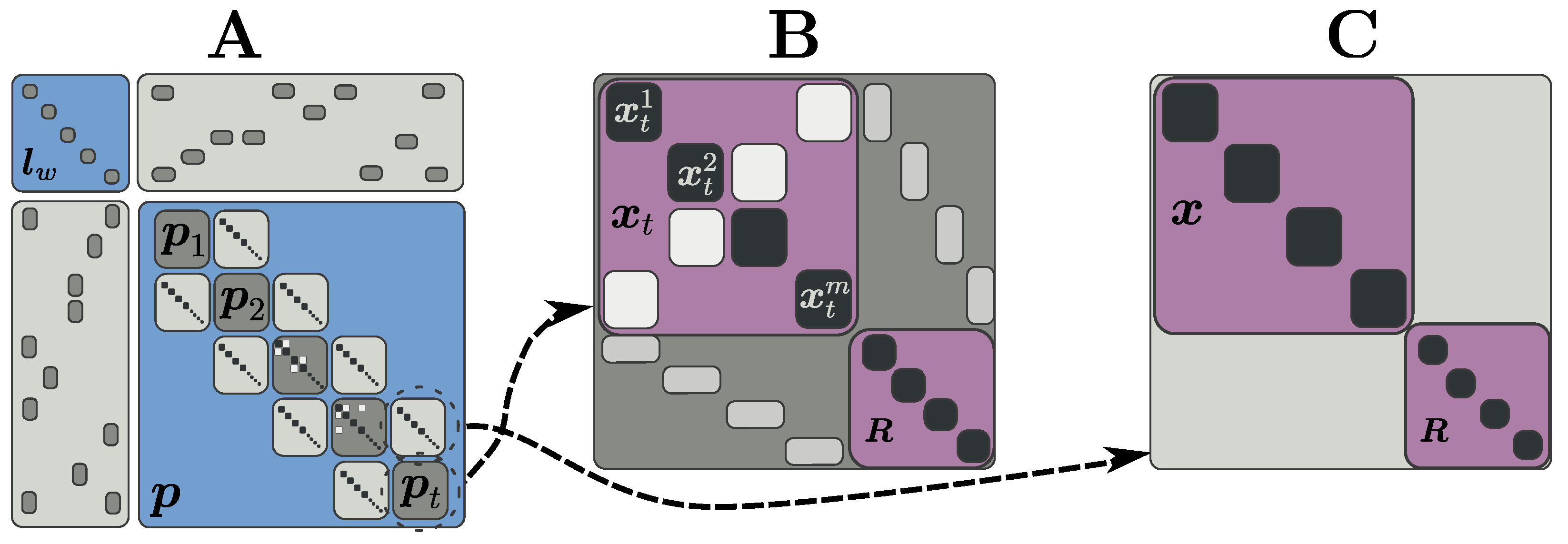
Figure 3. The structure of the total FIM, depicted as the symmetric matrix (A). The upper-left block matrix of (A) represents the FIM of visual feature, which is block-diagonal. The lower-right block of (A) is a strip-like matrix, of which the diagonal part has the structure as (B), and the off-diagonal part has the structure as (C), which is block-diagonal. The non-zero elements of the upper-right block matrix of (A) indicate the visibility of the corresponding visual feature and UAV.
Drones 07 00651 g003
From the above analysis, we can see that the structure of the FIM has some common properties with a pose graph and that the non-zero element reflects a valid measurement. For the partial FIM I IN , it is equivalent to the one for a pose graph in which only the consecutive frames of the same UAV are connected. Nevertheless, compared to the FIM for pose-graph SLAM, which only contains UAV states, our form can reflect the uncertainty of visual features.
The number of visual features grows fast over time; thus, analyzing such a big matrix becomes intractable. A practical solution is to split the states of visual features out of the total estimation states. The equivalent Fisher information matrix (EFIM) is a useful tool to evaluate the estimation performance for a subset of states by using the Schur complement trick [11]. By definition, the EFIM for UAV states ϑ is given by
J e ( ϑ ) = I ϑ I l w ϑ I l w 1 I l w ϑ
The dimension of J e ( ϑ ) is 3 M T × 3 M T in the 2-D case and is invariant to the visual feature number. Like the FIM structure, we can also partition the total EFIM into three parts:
J e ( ϑ ) = J e VF ( ϑ ) + J e IN ( ϑ ) + J e RA ( ϑ )
where J e IN ( x ) and J e R A ( x ) are simply the submatrices of I IN and I RA , respectively. We evaluate the submatrices of J e VF ( ϑ ) for position, i.e., J e VF ( x ) . Without loss of generality, we consider a scenario which contains a single time epoch and multiple UAVs. The multi-epoch scenario can be analyzed using the same method with state-reordering. According to Equation (27), the position-related EFIM by the visual feature measurement can be readily written as
J e VF ( x ) = I x VF ( I l w , x VF ) T I l w 1 I l w , x VF
Substituting the expressions of the above symbols in Equation (29), the following statements are readily proved:
  • J e VF ( x ) is a sparse-positive semidefinite matrix, and the non-zero block [ J e VF ( x ) ] m , n indicates that m-th and n-th UAV have common visibility for some visual features.
  • J e VF ( x ) is harmonic, i.e.,
    m M [ J e VF ( x ) ] m , n = 0
We can prove that these properties also apply to the multi-epoch scenario. The above analysis implies that J e VF ( x ) is an extension version of a Laplacian matrix, which can be exploited for trajectory optimization [28].

4.3. CRLB for Visual–Inertial–Range Cooperative Localization

CRLB reflects the covariance bounds that an unbiased estimator can reach. Referring to [25,30], if the signal-to-noise ratio (SNR) is large enough, the CRLB for the 2-D case has the same expression as the one in the Cartesian coordination, i.e.,
C ( θ θ ) I 2 D 1 ( θ θ )
θ θ , which means that the states set θ is assumed to be known. For example, θ = { l w 1 } means that the first visual feature is assumed to be an anchor. Meanwhile, in the 3-D case, due to the unflatness property of manifold R 3 × SO ( 3 ) , the CRLB is not just the inverse of EFIM. However, according to [25,30], we can still approximate CRLB with the inverse of EFIM when the noise is relatively small.
However, due to the massive visual feature amount, it is preferred to only evaluate the CRLB for UAV states ϑ . We can use the inversion of the EFIM to evaluate the performance bound for ϑ , i.e.,
C ( ϑ ϑ ) J e 1 ( ϑ ϑ )

5. Numerical Results

5.1. Correctness and Reachability of the CRLB

To evaluate the correctness and reachability of the CRLB, we construct some datasets with ground truth. Then, some measurement noises are applied based on the above assumptions. The noises that obey isotropic Langevin distribution are generated by the method described in [35].
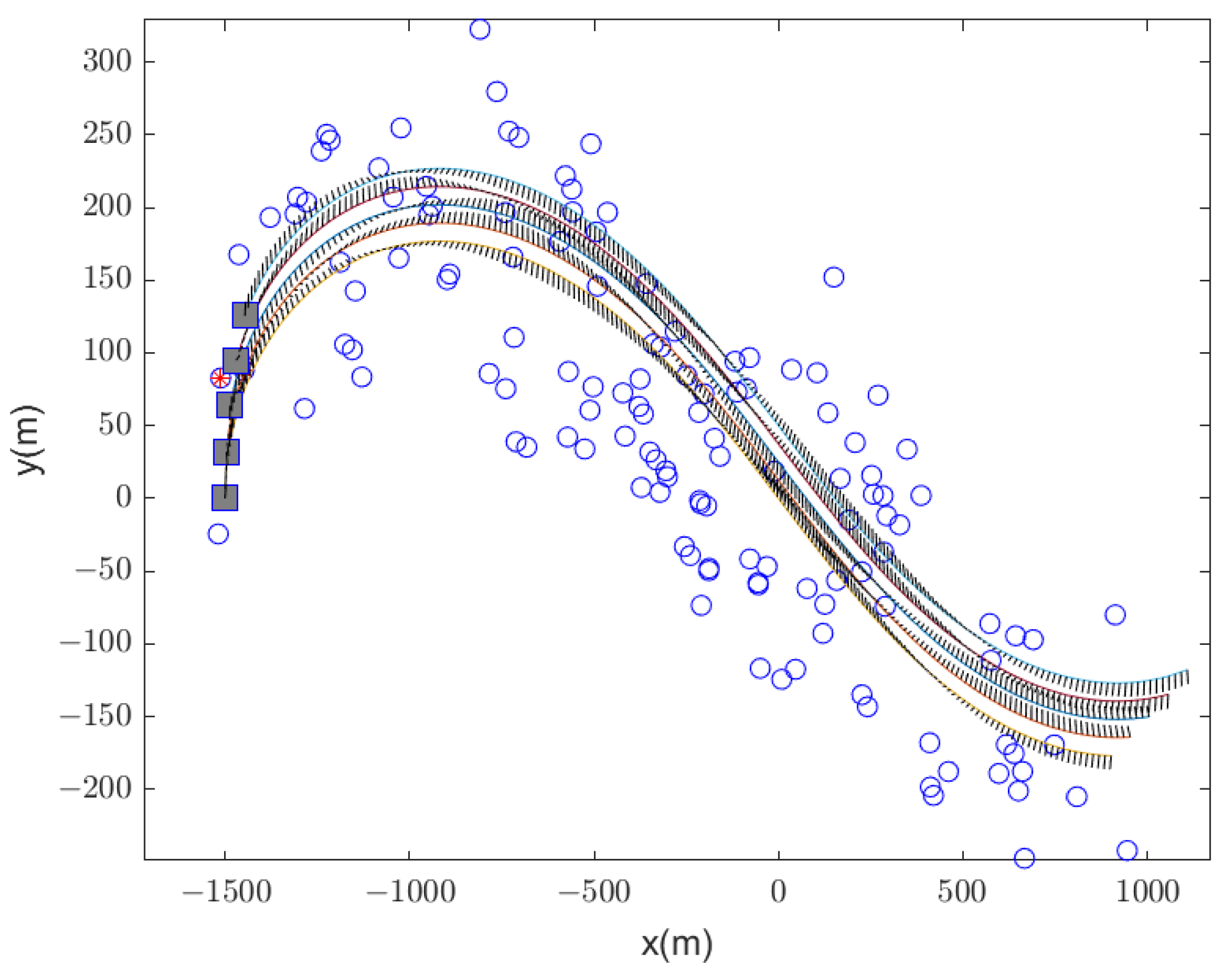
We simulate M = 5 UAVs to move along the lemniscate trajectory in 2-D space, as shown in Figure 4, denoted as Scenario 1. The time epoch T is set to 200. Each trajectory has a different initial position. The heading for each UAV is an integration of a normalized–distributed heading velocity. A total of 500 visual features are randomly generated around these trajectories. The FOV of the camera mounted on the UAV is set to 90 and f c = 250 pixel and σ u = 0.5 pixel . The range link is established between UAVs when their distance is less than 100 m , and its std σ z is set to 0.05 m . For the state transition measurement, we set κ i , j m = 50 and σ i , j = 0.1 m for all i , j , m .
Firstly, we evaluate the trajectory estimation performance for validating the correctness and reachability of the CRLB. We model the estimation problem as a classical bundle-adjustment problem. Then, the open-source Ceres Solver is exploited to solve this nonlinear least squares (NLS) optimization problem. A trust region method with a sparse normal Cholesky decomposition is applied as the optimization method. The initial point for this nonlinear optimization is set around the ground truth, by adding a small random value.
The root mean square error (RMSE) computed by N Monte Carlo simulations is used to evaluate the estimator performance, which is defined as
RMSE t m = 1 N i = 1 N i t m ¯ t m 2 2
“∗” stands for the UAV states, i.e., the position or rotation state. ¯ is the ground truth of ∗. The Root CRLB (rCRLB) of UAV states is calculated with the first four known visual feature positions. The rCRLB can be calculated as the square root of the trace of CRLB for the corresponding states. For example, the rCRLB of position state x j m is
rCRLB ( x j m ) = tr ( C x j m )
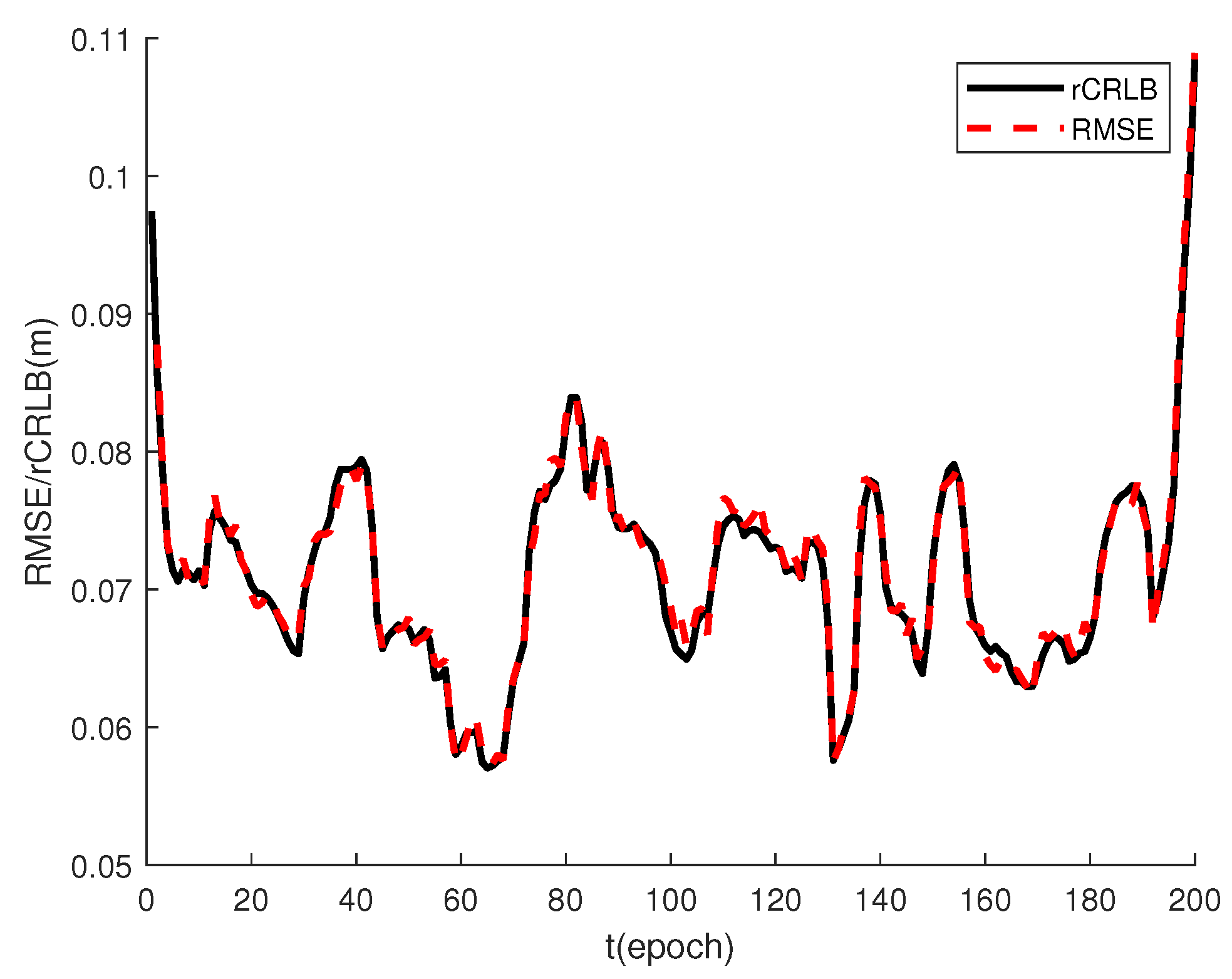
Firstly, the correctness and reachability of the performance bound in the 2-D case are evaluated, the results of which are shown in Figure 5, Figure 6 and Figure 7. For the first UAV, the rCRLB and RMSE are shown in Figure 5. As Figure 5 shows, the rCRLB and RMSE of the position state are almost equal. The mean difference between rCRLB and RMSE, i.e., | rCRLB RMSE | over time is 9.54 × 10 4 m , and the relative difference between them is only 1.10 % . This indicates that the CRLB is reachable using the NLS algorithm.
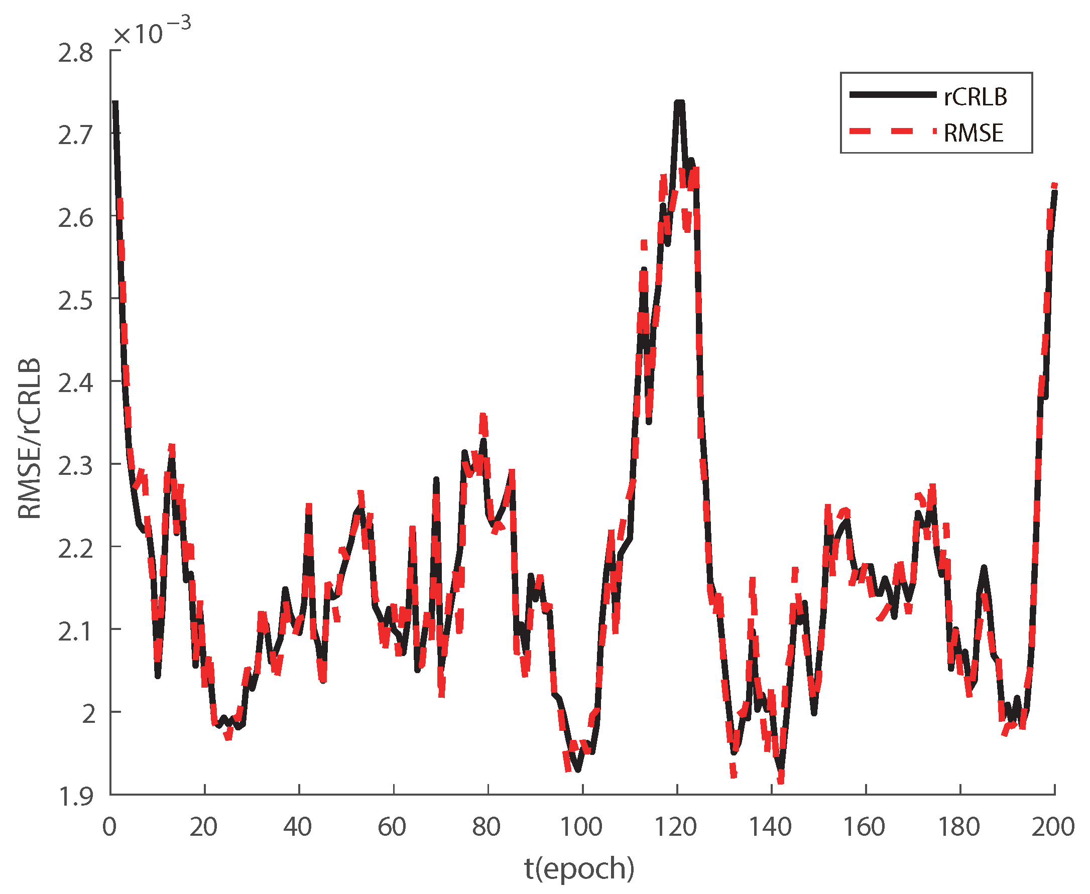
The rCRLB and RMSE for rotation are shown in Figure 6. The relative difference between the rCRLB and RMSE of rotation state is 2.02 % .
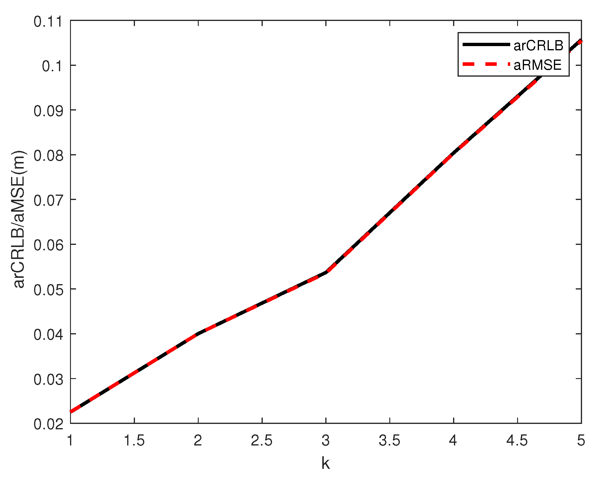
We also evaluate the CRLB reachability with respect to the noise change. We define a noise magnitude parameter k, and the noise parameters σ u , σ r , σ y , and κ are then changed to k σ u , k σ r , σ y , and 1 k κ , respectively. The average rCRLB (arCRLB) and average RMSE (aRMSE) for different ks are compared. The aRMSE is defined as
aRMSE m = 1 T t = 1 T RMSE t m
The comparison result is shown as Figure 7. The average difference between arCRLB and aRMSE over ks is 0.71 % . This shows that, for a relatively large noise, the CRLB is still reachable.
Then, we evaluate the reachability of the performance bound in the 3-D case. In this case, the trajectories of the UAVs are lemniscates with different heights, and all other parameters are the same as in the 2-D case. The 3-D trajectories and landmarks are shown in Figure 8.
Same as for the 2-D case, we compare the theoretic rCRLB and RMSE of NLS estimation using the Ceres Solver. With reference to the comparison results presented in Figure 9 and Figure 10, we can conclude that the CRLB of the UAV states can also be reached by NLS solver with smaller initial errors.

5.2. The Effect of the Visual Feature for CL

The loop closure is a powerful method in SLAM. It is performed when some visual features are covisible for two or more state factors. It can greatly reduce the long-term cumulative errors. In order to evaluate the effectiveness of the visual feature measurement for CL, we construct several simulations in the 2-D case as follows. We create simulation scenarios with/without visual loop closure, and then evaluate these absolute and relative position errors, respectively.
In contrast to absolute error, a relative position error only considers the error among UAVs. Therefore, it is useful to evaluate the accuracy of the formation. When the position error is relatively small, we can use the constraint CRLB to describe the relative positioning performance, which is given by [36]
C c = U c ( U c J e U c ) 1 U c
where J e is the EFIM for the position states, i.e., { x t m } t = 1 , 2 , , T m = 1 , 2 , , M . U c is a semiunitary matrix whose columns form an orthonormal basis for the nullspace of the relative position function gradient U N C , making U NC U c = 0 . In 2-D space, U N C can be formulated as
U NC = v x v y v ϕ v x = 1 0 1 0 v y = 0 1 0 1 v ϕ = ( y 1 y ¯ ) ( x 1 x ¯ ) ( y 2 y ¯ ) ( x 2 x ¯ )
In which x 1 and y 1 are the two components for the position state x 1 . x ¯ and y ¯ are x- and y- components for the centroid of the UAVs. Once U NC is constructed, U c can be calculated with the Gram–Schmidt process.
Firstly, we evaluate the effect of visual information with closure loop for the scenario depicted in Figure 4. The CRLBs with and without visual features are calculated.
The result shown in Figure 11 indicates that the position state error is greatly reduced when visual features are available. With loop closure, UAVs are able to determine the relative pose errors with earlier states, which makes the error lesser.
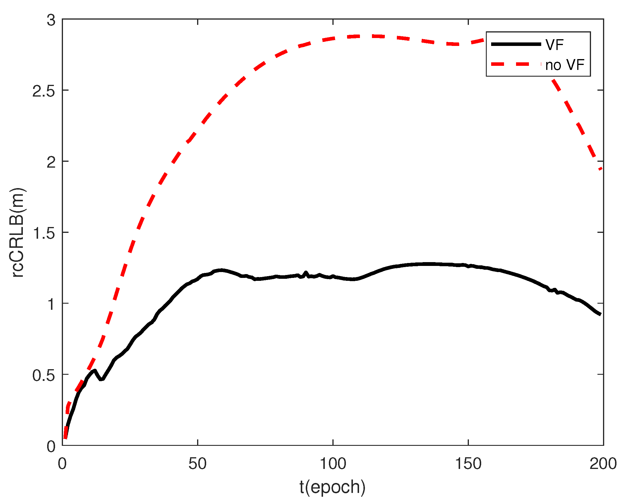
The constraint CRLB in this scenario is then evaluated. C c is calculated for each time epoch, denoted as C c ( t ) . After that, the square root of ( C c ( t ) ) , rcCRLB , is calculated as shown in Figure 12.
We can see that, when visual information is available, the constraint CRLB is also reduced, which signals the improvement in the formation accuracy. Unlike rCRLB, which diverges without visual information, rcCRLB retains a relatively small value. This is because UAVs can use the ranging information to maintain a stable relative formation.
Another scenario denoted as Scenario 3 for non-loopclosure is also constructed, in which the UAV trajectories are shown, as in Figure 13, whose length along the x-axis is more than 2 km.
With a long trajectory, UAVs are unable to see previous visual features older than a certain time, which prevents loop closure with a long period.
As Figure 14 shows, the rCRLB for this scenario diverges both with and without visual features. This is because the absolute localization of the UAV is unobservable with visual–inertial–range measurement. When no loopclosure is present, the UAV cannot reduce the localization uncertainty by the visual feature constraint either. Nevertheless, visual information greatly mitigates the divergence of the position error. With visual information, rCRLB is 63.7 m at t = 200 , whereas it becomes 518.2 m when visual information is neglected.
Figure 15 shows that, even without loop closure, visual features can still provide rich and effective information for formation. The average rcCRLB is 2.35 m without visual information, while it reduces to 1.07 m when visual information is added. It is worth noting that, at end of the time epoch, the rcCRLBs for both situations start to decrease. That is due to the fact that the relative position configuration of UAVs changes, which increases the total information of range measurements.

5.3. The Effect of the Range Measurement for CL: The Scenario of Large Baseline Cooperative Flying at High Altitudes

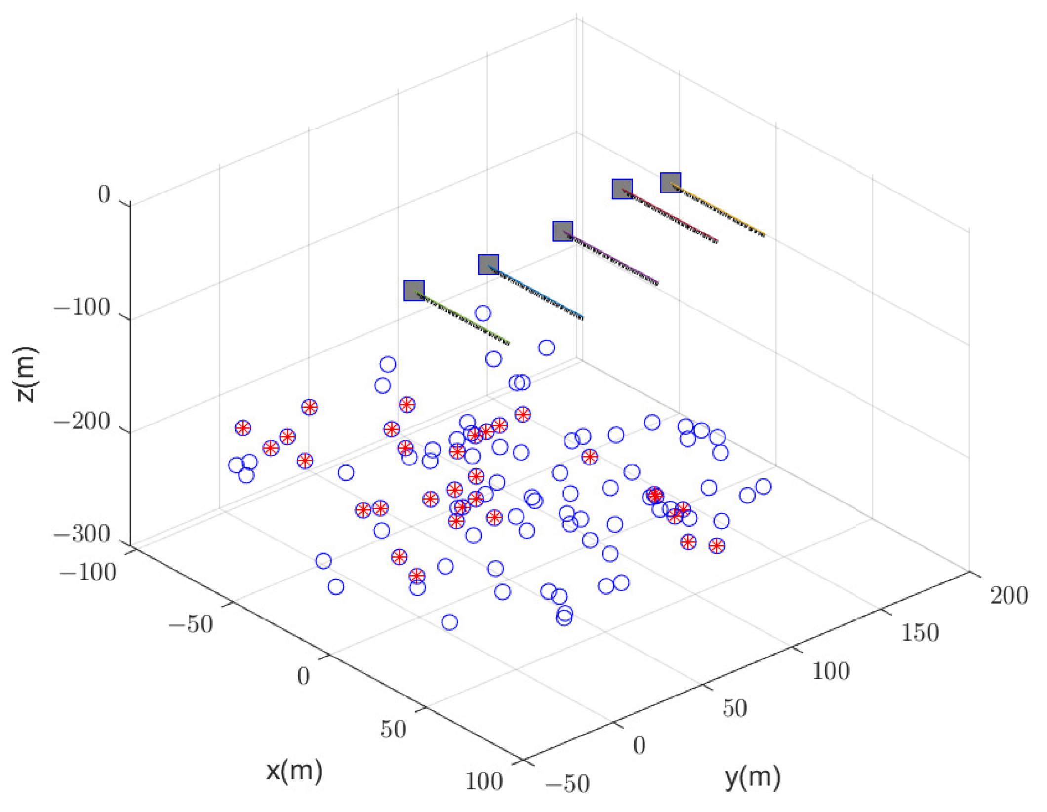
Cooperative flight at high altitudes is a valuable application as it enables the UAV swarm to efficiently cover a large area simultaneously. However, the conventional method of VIO for single UAV positioning at high altitudes faces significant challenges. This is primarily due to its reliance on accurate visual feature triangulation. The accurate estimation of a larger scene depth requires a wider range of motion to achieve a significant triangulation angle, which is crucial for a precise VIO system [37]. However, relying solely on the IMU for estimating this extended range results in excessive noise accumulation, leading to compromised positioning performance. In light of this, our following experiment demonstrates that the addition of range measurements between UAVs can significantly improve the positioning performance, and shows how the proposed metric helps us to analyze and optimize the measurement strategy for CL in the UAV swarm.
We construct a scenario in which a UAV swarm is flying at high altitude, as shown in Figure 16. This swarm consists of five UAVs flying at an altitude of approximately 250 m. Each pair of UAVs is spaced approximately 30 m apart.
To simulate the poor ego-motion estimation of high-altitude flying, we set the noise of the pose-graph measurement rather large, i.e., κ i , j m = 50 and σ i , j = 5 m for all i , j , m , and the FOV of the camera is set to 20 . σ u and σ z are set to 1 pixel and 0.05 m , respectively. Other parameters remain the same as above. Then, we evaluate the position performance using the CRLB metric, with and without the range measurements.
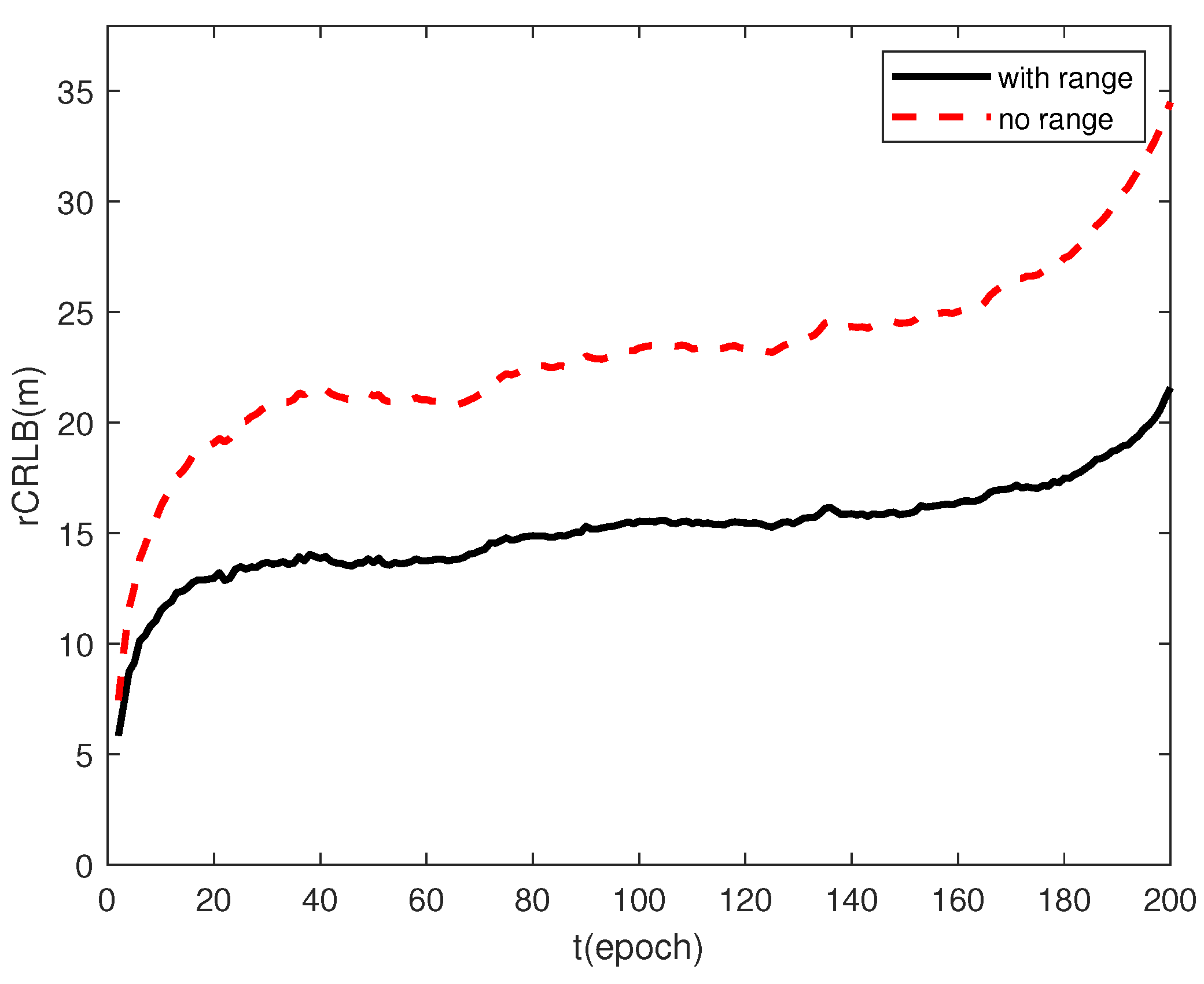
The rCRLBs of position and rotation states for UAV 1 are shown in Figure 17 and Figure 18, respectively. Figure 17 and Figure 18 show that, with the assistant or range measurements, the average rCLRB of position state for UAV 1 decreases by 34.5 % (from 23.1 m to 15.1 m ), while the average rCLRB of rotation state decreases by 34.0 % (from 0.134 to 0.0883 ). This proves that the range measurement can greatly improve the estimation accuracy when the other localization information is deficient.

6. Conclusions

In this paper, we first build the FIM of the visual–inertial–range cooperative localization in the product manifold R n × SO ( n ) . Then, some important properties of the FIM are analyzed, such as sparsity and harmonic structure, which are essential for practical application to analyze the performance of cooperative localization. Through a series of numerical simulations, we prove the effectiveness of this performance analysis tool and conclude that visual features can greatly improve CL performance, both in terms of absolute and relative localization accuracy. This shows that our performance analysis tool can be used in measurement selection for resource-constraint CL, which will be the subject of our future work.
While this paper focuses on the fundamental performance of CL with environment visual features for UAV swarms, it can be easily modified to be applicable to CL utilizing other environment information, such as LiDAR and event camera data.

Author Contributions

Conceptualization, J.L.; Methodology, J.L.; Software, J.L.; Validation, J.L.; Formal analysis, J.L.; Data curation, D.T. and H.Z.; Writing—review and editing, C.L.; Visualization, S.L.; Project administration, X.X. All authors have read and agreed to the published version of the manuscript.

Funding

Research was funded by the National Natural Science Foundation of China under Grant 62001494.

Data Availability Statement

Not applicable.

Conflicts of Interest

The authors declare no conflict of interest.

References

  1. Kaufmann, E.; Bauersfeld, L.; Loquercio, A.; Müller, M.; Koltun, V.; Scaramuzza, D. Champion-Level Drone Racing Using Deep Reinforcement Learning. Nature 2023, 620, 982–987. [Google Scholar] [CrossRef]
  2. Loquercio, A.; Kaufmann, E.; Ranftl, R.; Müller, M.; Koltun, V.; Scaramuzza, D. Learning High-Speed Flight in the Wild. Sci. Robot. 2021, 6, eabg5810. [Google Scholar] [CrossRef] [PubMed]
  3. Yan, C.; Xiang, X.; Wang, C.; Lan, Z. Flocking and Collision Avoidance for a Dynamic Squad of Fixed-Wing UAVs Using Deep Reinforcement Learning. In Proceedings of the 2021 IEEE/RSJ International Conference on Intelligent Robots and Systems (IROS), Prague, Czech Republic, 27 September–1 October 2021; pp. 4738–4744. [Google Scholar] [CrossRef]
  4. Yan, C.; Wang, C.; Xiang, X.; Lan, Z.; Jiang, Y. Deep Reinforcement Learning of Collision-Free Flocking Policies for Multiple Fixed-Wing UAVs Using Local Situation Maps. IEEE Trans. Ind. Inform. 2022, 18, 1260–1270. [Google Scholar] [CrossRef]
  5. Lu, K.; Hu, R.; Yao, Z.; Wang, H. Onboard Distributed Trajectory Planning through Intelligent Search for Multi-UAV Cooperative Flight. Drones 2023, 7, 16. [Google Scholar] [CrossRef]
  6. Yang, Y.; Xiong, X.; Yan, Y. UAV Formation Trajectory Planning Algorithms: A Review. Drones 2023, 7, 62. [Google Scholar] [CrossRef]
  7. Chung, S.J.; Paranjape, A.A.; Dames, P.; Shen, S.; Kumar, V. A Survey on Aerial Swarm Robotics. IEEE Trans. Robot. 2018, 34, 837–855. [Google Scholar] [CrossRef]
  8. Sun, Y.; Tan, Q.; Yan, C.; Chang, Y.; Xiang, X.; Zhou, H. Multi-UAV Coverage through Two-Step Auction in Dynamic Environments. Drones 2022, 6, 153. [Google Scholar] [CrossRef]
  9. Zhou, X.; Zhu, J.; Zhou, H.; Xu, C.; Gao, F. EGO-Swarm: A Fully Autonomous and Decentralized Quadrotor Swarm System in Cluttered Environments. In Proceedings of the 2021 IEEE International Conference on Robotics and Automation (ICRA), Xi’an, China, 30 May–5 June 2021; pp. 4101–4107. [Google Scholar] [CrossRef]
  10. Liu, Y.; Wang, Y.; Wang, J.; Shen, Y. Distributed 3D Relative Localization of UAVs. IEEE Trans. Veh. Technol. 2020, 69, 11756–11770. [Google Scholar] [CrossRef]
  11. Shen, Y.; Win, M.Z. Fundamental Limits of Wideband Localization— Part I: A General Framework. IEEE Trans. Inf. Theory 2010, 56, 4956–4980. [Google Scholar] [CrossRef]
  12. Dai, W.; Shen, Y.; Win, M.Z. Distributed Power Allocation for Cooperative Wireless Network Localization. IEEE J. Sel. Areas Commun. 2015, 33, 28–40. [Google Scholar] [CrossRef]
  13. Lai, J.; Zhou, Y.; Lin, J.; Cong, Y.; Yang, J. Cooperative Localization Based on Efficient Covariance Intersection. IEEE Commun. Lett. 2019, 23, 871–874. [Google Scholar] [CrossRef]
  14. Caceres, M.A.; Penna, F.; Wymeersch, H.; Garello, R. Hybrid Cooperative Positioning Based on Distributed Belief Propagation. IEEE J. Sel. Areas Commun. 2011, 29, 1948–1958. [Google Scholar] [CrossRef]
  15. Funabiki, N.; Morrell, B.; Nash, J.; Agha-mohammadi, A.-a. Range-Aided Pose-Graph-Based SLAM: Applications of Deployable Ranging Beacons for Unknown Environment Exploration. IEEE Robot. Autom. Lett. 2021, 6, 48–55. [Google Scholar] [CrossRef]
  16. Etzlinger, B.; Wymeersch, H.; Springer, A. Cooperative Synchronization in Wireless Networks. IEEE Trans. Signal Process. 2014, 62, 2837–2849. [Google Scholar] [CrossRef]
  17. Ellingson, G.; Brink, K.; McLain, T. Relative Visual-Inertial Odometry for Fixed-Wing Aircraft in GPS-denied Environments. In Proceedings of the 2018 IEEE/ION Position, Location and Navigation Symposium (PLANS), Monterey, CA, USA, 23–26 April 2018; pp. 786–792. [Google Scholar] [CrossRef]
  18. Xu, L.; Shen, X.; Wang, L.; Shen, Y. A Distributed Relative Localization Scheme Based on Geometry Merging Priority. In Proceedings of the GLOBECOM 2022—2022 IEEE Global Communications Conference, Rio de Janeiro, Brazil, 4–8 December 2022; IEEE: Piscataway, NJ, USA, 2022; pp. 3995–4000. [Google Scholar] [CrossRef]
  19. Wang, N.; Chen, T.; Liu, S.; Wang, R.; Karimi, H.R.; Lin, Y. Deep Learning-Based Visual Detection of Marine Organisms: A Survey. Neurocomputing 2023, 532, 1–32. [Google Scholar] [CrossRef]
  20. Campos, C.; Elvira, R.; Rodríguez, J.J.G.; Montiel, J.M.; Tardós, J.D. ORB-SLAM3: An Accurate Open-Source Library for Visual, Visual-Inertial and Multi-Map SLAM. arXiv 2020, arXiv:2007.11898. [Google Scholar] [CrossRef]
  21. Mourikis, A.I.; Roumeliotis, S.I. A Multi-State Constraint Kalman Filter for Vision-Aided Inertial Navigation. In Proceedings of the 2007 IEEE International Conference on Robotics and Automation, Roma, Italy, 10–14 April 2007; IEEE: Piscataway, NJ, USA, 2007; pp. 3565–3572. [Google Scholar]
  22. Xu, H.; Zhang, Y.; Zhou, B.; Wang, L.; Yao, X.; Meng, G.; Shen, S. Omni-Swarm: A Decentralized Omnidirectional Visual–Inertial–UWB State Estimation System for Aerial Swarms. IEEE Trans. Robot. 2022, 38, 3374–3394. [Google Scholar] [CrossRef]
  23. Lajoie, P.Y.; Ramtoula, B.; Wu, F.; Beltrame, G. Towards Collaborative Simultaneous Localization and Mapping: A Survey of the Current Research Landscape. Field Robot. 2022, 2, 971–1000. [Google Scholar] [CrossRef]
  24. Zhang, Z.; Scaramuzza, D. Beyond Point Clouds: Fisher Information Field for Active Visual Localization. In Proceedings of the 2019 International Conference on Robotics and Automation (ICRA), Montreal, QC, Canada, 20–24 May 2019; pp. 5986–5992. [Google Scholar] [CrossRef]
  25. Chen, Y.; Huang, S.; Zhao, L.; Dissanayake, G. Cramér–Rao Bounds and Optimal Design Metrics for Pose-Graph SLAM. IEEE Trans. Robot. 2021, 37, 627–641. [Google Scholar] [CrossRef]
  26. Khosoussi, K.; Giamou, M.; Sukhatme, G.S.; Huang, S.; Dissanayake, G.; How, J.P. Reliable Graphs for SLAM. Int. J. Robot. Res. 2019, 38, 260–298. [Google Scholar] [CrossRef]
  27. Khosoussi, K.; Huang, S.; Dissanayake, G. Novel Insights into the Impact of Graph Structure on SLAM. In Proceedings of the 2014 IEEE/RSJ International Conference on Intelligent Robots and Systems, Chicago, IL, USA, 14–18 September 2014; IEEE: Piscataway, NJ, USA, 2014; pp. 2707–2714. [Google Scholar] [CrossRef]
  28. Chen, Y.; Zhao, L.; Lee, K.M.B.; Yoo, C.; Huang, S.; Fitch, R. Broadcast Your Weaknesses: Cooperative Active Pose-Graph SLAM for Multiple Robots. IEEE Robot. Autom. Lett. 2020, 5, 2200–2207. [Google Scholar] [CrossRef]
  29. Kontitsis, M.; Theodorou, E.A.; Todorov, E. Multi-Robot Active SLAM with Relative Entropy Optimization. In Proceedings of the 2013 American Control Conference, Washington, DC, USA, 17–19 June 2013; IEEE: Piscataway, NJ, USA, 2013; pp. 2757–2764. [Google Scholar] [CrossRef]
  30. Boumal, N.; Singer, A.; Absil, P.A.; Blondel, V.D. Cramér–Rao Bounds for Synchronization of Rotations. Inf. Inference A J. IMA 2014, 3, 1–39. [Google Scholar] [CrossRef]
  31. Boumal, N. On Intrinsic Cramér-Rao Bounds for Riemannian Submanifolds and Quotient Manifolds. IEEE Trans. Signal Process. 2013, 61, 1809–1821. [Google Scholar] [CrossRef]
  32. Engel, J.; Sturm, J.; Cremers, D. Semi-Dense Visual Odometry for a Monocular Camera. In Proceedings of the 2013 IEEE International Conference on Computer Vision, Sydney, Australia, 1–8 December 2013; IEEE: Piscataway, NJ, USA, 2013; pp. 1449–1456. [Google Scholar] [CrossRef]
  33. Wendel, A.; Maurer, M.; Graber, G.; Pock, T.; Bischof, H. Dense Reconstruction On-the-Fly. In Proceedings of the 2012 IEEE Conference on Computer Vision and Pattern Recognition, Providence, RI, USA, 16–21 June 2012; pp. 1450–1457. [Google Scholar] [CrossRef]
  34. Qin, T.; Li, P.; Shen, S. Vins-Mono: A Robust and Versatile Monocular Visual-Inertial State Estimator. IEEE Trans. Robot. 2018, 34, 1004–1020. [Google Scholar] [CrossRef]
  35. Best, D.J.; Fisher, N.I. Efficient Simulation of the von Mises Distribution. J. R. Stat. Soc. Ser. C (Appl. Stat.) 1979, 28, 152–157. [Google Scholar] [CrossRef]
  36. Ash, J.N.; Moses, R.L. On the Relative and Absolute Positioning Errors in Self-Localization Systems. IEEE Trans. Signal Process. 2008, 56, 5668–5679. [Google Scholar] [CrossRef]
  37. Karrer, M.; Chli, M. Distributed Variable-Baseline Stereo SLAM from Two UAVs. In Proceedings of the 2021 IEEE International Conference on Robotics and Automation (ICRA), Xi’an, China, 30 May–5 June 2021; pp. 82–88. [Google Scholar] [CrossRef]
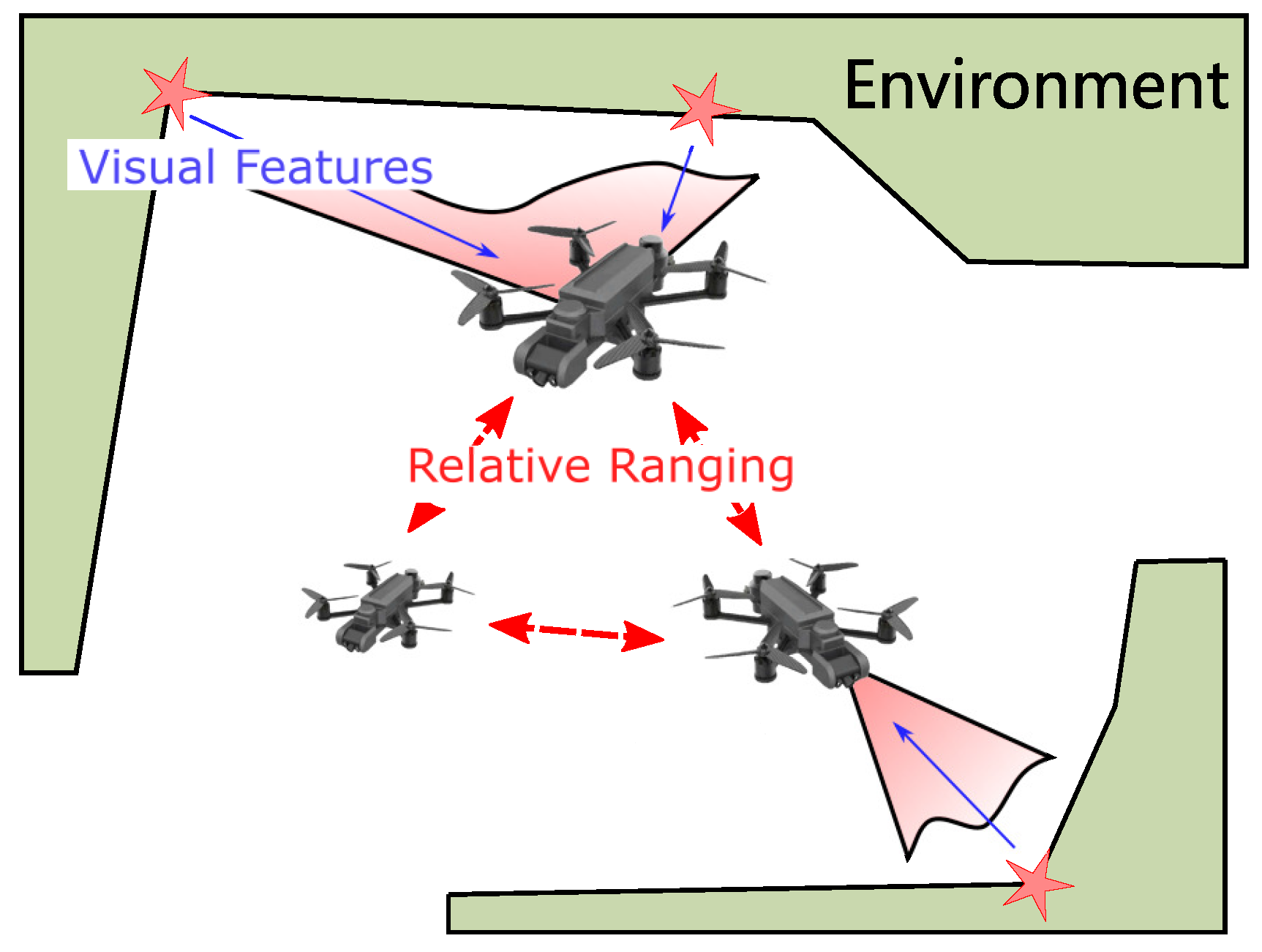
Figure 1. Diagram of cooperative localization (CL) with support of environment visual features. The small UAVs use their cameras to extract visual features in the environment, and establish range links with others. The static visual features can be recognized as an anchor, which makes the UAV group be infrastructure-less.
Drones 07 00651 g001
Figure 2. The graph representation for the measurement model. The black thick line, the black thin line, and the red line stand for the inertial, visual, and range measurement, respectively.
Drones 07 00651 g002
Figure 4. The trajectories and visual features of simulation settings of Scenario 1. Five UAVs move along their lemniscate trajectories, in which the small squares are the initial positions. The heading for each position is represented as a black short line. The blue circles are visual features, of which with red stars indicate the visibility for the initial position.
Drones 07 00651 g004
Figure 5. The absolute rCRLB and RMSE of position state with N = 1000 in Scenario 1. The black line is the position rCRLB of the first Ulyanovsk, while the red dotted line represents the RMSE for corresponding states.
Drones 07 00651 g005
Figure 6. The absolute rCRLB and RMSE of rotation state with N = 1000 in Scenario 1.
Drones 07 00651 g006
Figure 7. The absolute arCRLB and aRMSE of position state with different noise magnitudes in Scenario 1. The black line is the position arCRLB of the first UAV, while the red dotted line represents the aRMSE for corresponding states.
Drones 07 00651 g007
Figure 8. The trajectories and visual features of simulation settings the 3-D scenario, named Scenario 2. 5 UAVs move along their lemniscate trajectories, in which the small squares are the initial positions.
Drones 07 00651 g008
Figure 9. The absolute rCRLB and RMSE of position state with N = 1000 in Scenario 2. The black line is the position rCRLB of the first UAV, while the red dotted line represents for the RMSE for corresponding states.
Drones 07 00651 g009
Figure 10. The absolute rCRLB and RMSE of rotation state with N = 1000 in Scenario 2.
Drones 07 00651 g010
Figure 11. The absolute rCLRBs of position state with and without visual information in Scenario 1.
Drones 07 00651 g011
Figure 12. Root square of constraint CRLB with and without visual information in Scenario 1, which indicates the relative position error among UAVs.
Drones 07 00651 g012
Figure 13. Scenario 3: UAV trajectories for non-loopclosure scenario.
Drones 07 00651 g013
Figure 14. The absolute rCLRBs of position states with and without visual information in Scenario 3.
Drones 07 00651 g014
Figure 15. Root square of constraint CRLB with and without visual information for Scenario 3, which indicates the relative localization error among UAVs.
Drones 07 00651 g015
Figure 16. The scenario of large baseline cooperative flying at high altitudes. The blue circles represent visual features on the ground, and the red asterisks indicate the features that are co-visible for more than 2 UAVs.
Drones 07 00651 g016
Figure 17. The rCRLB of position state for UAV 1 in the large-baseline scenario.
Drones 07 00651 g017
Figure 18. The rCRLB of rotation state for UAV 1 in the large-baseline scenario.
Drones 07 00651 g018
Disclaimer/Publisher’s Note: The statements, opinions and data contained in all publications are solely those of the individual author(s) and contributor(s) and not of MDPI and/or the editor(s). MDPI and/or the editor(s) disclaim responsibility for any injury to people or property resulting from any ideas, methods, instructions or products referred to in the content.