Small Unmanned Aircraft Systems and Agro-Terrestrial Surveys Comparison for Generating Digital Elevation Surfaces for Irrigation and Precision Grading

Abstract

Advances in remote sensing and small unmanned aircraft systems (sUAS) have been applied to various precision agriculture applications. However, there has been limited research on the accuracy of real-time kinematic (RTK) sUAS photogrammetric elevation surveys, especially in preparation for precision agriculture practices that require precise topographic surfaces, such as increasing irrigation system efficiency. These practices include, but are not limited to, precision land grading, placement of levees, multiple inlet rice irrigation, and computerized hole size selection for furrow irrigation. All such practices rely, in some way, on the characterization of surface topography. While agro-terrestrial (ground-based) surveying is the dominant method of agricultural surveying, aerial surveying is emerging and attracting potential early adopters. This is the first study of its kind to assess the accuracy, precision, time, and cost efficiency of RTK sUAS surveying in comparison to traditional agro-terrestrial techniques. Our findings suggest sUAS are superior to ground survey methods in terms of relative elevation and produce much more precise raster surfaces than ground-based methods. We also showed that this emergent technology reduces costs and the time it takes to generate agricultural elevation surveys.

1. Introduction

In Arkansas, approximately 80% of irrigation water comes from groundwater [1]. The Mississippi River Valley Alluvial Aquifer (MRVAA) supplies most irrigation applied in the Lower Mississippi River Basin [2]. Currently, the MRVAA has regions of extensive decline due to geology and extensive agricultural production systems [3]. To enhance the sustainability of the MRVAA, producers attempt to improve irrigation water use efficiency by implementing conservation practices such as multiple inlet irrigation in rice (Oryza sativa) and computerized hole size selection for furrow irrigation of corn (Zea mays), peanuts (Arachis hypogaea), soybeans (Glycine max), and cotton (Gossypium herbaceum). However, these practices require fields to be precision-graded.

A technological solution to increasing food production as well as reducing various inputs is the implementation of precision agriculture (PA) techniques, including emerging autonomous technologies. Current farm machinery is commonly equipped with PA technology, including RTK-GNSS receivers, variable rate technology (VRT), automatic steering, remote sensing of plant health, etc. However, the cost and complexity of technologies, including data management and interpretation, have been cited as barriers to precision agriculture adoption [4]. Another is the ever-increasing rate of change in PA technology, which has quickly advanced beyond the current farm labor skillset. This has resulted in a backlash against the adoption of new PA technologies, especially in regions with a tight labor market [5,6]. In locations where people have left rural areas for cities, farm labor is in short supply. The difficulty farmers have in hiring staff is exacerbated by the need for novel technical skills, which might be less common in rural settings. Sustainable returns on PA investments will be critical as further technological advancements occur [7]. Maybe even more importantly, the perceived value of the benefits of PA technology must exceed the added cost of the technology.

Precision land leveling or land grading in agriculture is the practice of changing a field’s topography to create the desired surface, affecting the water movement while improving irrigation and drainage efficiencies, therefore improving the effectiveness of cultivation operations [8]. The benefits associated with precision land leveling include improving surface drainage by eliminating low areas, reducing water ponding by adding grade to no-slope areas, and enhancing efficiency through uniform distribution, among others [9]. The initial leveling of a field could negatively impact soil conservation and erosion if not assessed carefully before land forming. The key to successful precision land leveling or grading is an accurate topographic survey, commonly accomplished using RTK-GNSS equipment.

An accurate topographic survey is crucial for effective water management in rice and other commodity crop production [10]. The topographic survey is conducted using either a grid-based pattern, an irregularly spaced pattern, or a combination of both [9]. Grid-based agro-terrestrial survey patterns are best suited for fields with relatively smooth elevation transitions throughout the field. In contrast, irregularly spaced agro-terrestrial patterns can often adequately define a field with abrupt elevation changes [9].

Several high-accuracy survey correction methods are known. RTK is the most commonly used method by NRCS [11]. Cellular network RTK (eRTK), also referred to as real-time network (RTN), produces centimeter-level accuracy using an internet connection through a cellular device [11]. Another cellular correction method is the virtual reference station (VRS). This involves the inverse distance weighting of the GPS error from its surroundings. Continuously operating reference stations (CORS) are used to correct readings taken at the rover location [11].

Agricultural land surveying identifies high- and low-elevation points to characterize field topography. This precedes the planning of an irrigation water management system [12]. Such elevation surveys are used to characterize the ability of a field to drain efficiently, estimate precision land grading costs, assess a field’s suitability for surface irrigation, or identify the need for pivot irrigation [12]. Another use of field topography is the placement of levees (contour and straight) for rice production. Agricultural surveyors in the Lower Mississippi River Basin (LMRB) typically employ a topographic survey method consisting of the following steps. First, the RTK-GNSS base is set over an unknown point. The RTK-GNSS rover is mounted to a vehicle such as a pickup truck or utility vehicle (UTV). Then, the agricultural surveyor drives the boundary, collecting points with x, y, and z coordinates. The agricultural surveyor employs a topographic survey style called “gridding” for data collection [11].

Agricultural applications employing relative elevation collection, processing, and utilization practices may not utilize GCPs. Such activities are often locally oriented and disconnected from elevation beyond the relevant local watershed. This is especially the case when laser technology is employed for agricultural surveying. Miao et al. discuss precision land leveling (PLL), a practice used in agriculture to change a field’s topographic surface to increase irrigation efficiency, using laser technology [8].

When surveying an agricultural field, an RTK-GNSS base station is often set up over an unknown position. This is due, in part, to the unlikely need for repeatability at an agricultural field site. In regions utilizing in-field irrigation levees such as the LMRB, it is common for farmers to survey fields on an annual basis. In these periodic surveys, they mark ridges or levees. Marking ridges is accomplished by dropping flags every 12–18 m along the topographically high locations. For levee creation, agricultural surveyors pull a small plow along an elevation contour to mark the levee location. Then, the farmer visually follows those marks as they pull a levee plow with a tractor.

Agricultural GNSS horizontal accuracies differ from those of engineering-grade survey equipment. For agricultural-grade equipment, Trimble Agriculture reported horizontal accuracies of <0.025 m for Radio RTK/Center Point RTK, Mobile RTK/Center Point RTK, and CenterPoint VRS [13]. John Deere states an accuracy of <0.025 m for Radio TRK/Center Point RTK [14], and Topcon lists an accuracy of <0.025–0.05 m for Radio TRK/Center Point RTK [15].

Table 1. Trimble correction networks across construction and engineering GNSS receivers [16].

GNSS Correction Source	Delivery Method	GNSS Horizontal Precision (m)	GNSS Vertical Precision RMS (m)	Initialization Time
Autonomous	Direct satellite	−1	1.5	N/A
SBAS—WAAS, EGNOS, etc.	Geostationary satellite	0.5	0.85	N/A
Trimble GNSS RTK Base Station	tUHF, cellular, WiFi	0.008 + 1.0 ppm	0.015 + 1.0 ppm	<8 s
Trimble VRS Now	Internet, cellular, regional	0.008 + 1.0 ppm	0.015 + 1.0 ppm	<8 s
CenterPoint RTX (Fast or Standard Subscription Level)	Geostationary satellite, internet, in certain defined geographic regions.	0.02	0.05	<1 or 15 min, depending on fast or standard subscription, and if available in a geographic region

reveals the regional availability, correction signal mode, horizontal accuracy, vertical accuracy, and initialization times for Trimble’s GNSS receiver solutions.

Table 2. Trimble R8s and Topcon HiPer SR antennas reported maximum accuracy in horizontal and vertical coordinates [17,18].

Manufacturer	RTK Horizontal Accuracy (m)	RTK Vertical Accuracy (m)
Trimble Engineering	0.008 + 1.0 ppm	0.015 + 1.0 ppm
Topcon Engineering	0.01 + 1.0 ppm	0.015 + 1.0 ppm

compares the maximum accuracy in horizontal and vertical dimensions of two specific engineering-grade antennas, that is, Trimble R8s and Topcon HiPer SR. These two engineering-quality antennas are state-of-the-art, providing centimeter-level accuracies horizontally and one-and-a-half centimeter-level accuracies vertically. Taken together, this information demonstrates why RTK is the primary method of collecting land surface elevation data for precision grading.

One variable component related to agricultural surveying for land grading is the gridding survey style. Gridding divides a field into equal grid squares to build a relative elevation model. The style of this grid varies depending on the RTK-GNSS manufacturer and individual surveyor preferences. For example, Topcon suggests a 30.5 m by 6.1 m grid pattern. Alternatively, Trimble recommends a 12 m by 1.5 m grid pattern, significantly increasing the amount of data collected. Furthermore, the survey style differs from one agricultural surveyor to another; this differs mainly by the spacing that the rover uses when driving across a field and the size of the land leveling equipment. Although agro-terrestrial surveys are the dominant method for a field’s topographic characterization, another method of generating an elevation surface is via small unmanned aerial systems (sUAS), which have gained significant attention recently [19].

An sUAS is currently defined by the Federal Aviation Administration (FAA) as “an unmanned aircraft weighing less than 25 kg at takeoff, including equipment; as well as associated equipment including communications equipment that controls the aircraft to ensure safe and efficient operation in the national airspace” [20]. The commercial use of sUAS has been growing in many industries [19]. Currently, there are two main categories of airframes for sUAS systems on the commercial market, that is, fixed-wing and rotary-wing sUAS. A sUAS is piloted manually by a human or autopiloted through GPS and inertial navigation systems (INS) technology [21].

One of the primary uses of sUAS technologies in agriculture is photogrammetric surveys. Such surveys are typically conducted over small areas of less than 3 km². As the photogrammetric process and sUAS technology continue to advance, the ability to produce a high-quality digital surface model (DSM) through a technique known as structure from motion (SfM) is emerging and is commercially available through Pix4Dmapper and Agisoft Photoscan [22].

A few decades ago, in photogrammetry, sUAS operators utilized a technique known as bundle block adjustment (BBA) and aerial triangulation (AT) to orient photos with relative accuracy using ground control points (GCPs). Another more contemporary technique is direct georeferencing (DG), which uses the sUAS GNSS to correct the photos rather than GCPs [22]. However, DG’s accuracy directly correlates to the accuracy of the consumer-grade sUAS GNSS receiver and is often at the meter level of accuracy [22]. Due to this relatively low level of precision from DG, sUAS mapping with GCPs is still a common practice today when using consumer-grade sUAS technologies.

The measurement of GCP coordinates is the most time-consuming operation of a sUAS survey [23]. As sUAS mapping and surveying equipment have evolved with more precision and accuracy, they appear to be a more efficient option for agricultural land surveying than traditional methods. For example, a team from Texas A&M University and USDA-NRCS assessed the abilities of sUAS for land leveling on an agricultural field [24]. The authors reported that the sUAS used in the study can assess the estimated ground height or performance of a land leveling project. Rogers et al. [25] compared sUAS LiDAR and four consumer-grade sUAS using SfM and AT for georeferencing. The literature continues to confirm that sUAS surveying is possible with AT and the use of GCPs. However, this practice is labor- and time-intensive and is not practical for kilometer-scale mapping projects.

A few published articles address the empirical accuracy capabilities of an RTK-enabled sUAS. Benassi et al. [26] utilized Photoscan Pro and Pix4D to assess the root mean square error (RMSE) of horizontal and vertical accuracies across four different RTK-GNSS configurations. This method drastically reduces survey time compared to the standard three or more GCPs for a sUAS survey mission. Forlani et al. [23] expanded on the Benassi et al. [26] research by including double the number of flights and adding correction networks, including CORS. Like Benassi et al. [26], Forlani et al. [23] achieved a RMSE of 0.03 m when using one GCP.

As sUAS equipment evolves, so does the associated GNSS equipment, resulting in more accurate sUAS systems for surveying. Rabah et al. [27] discuss another georeferencing approach using RTK-sUAS called direct georeferencing (DG). The DG method captures the natural position and orientation of a camera while taking digital images, allowing each pixel to be georeferenced to the Earth without GCPs [27]. This approach can reduce costs and time spent collecting data by eliminating the need for GCPs, reducing the lateral overlap of photos, and, thus, shortening the flight time required to collect data. The study, like many others, continues to illustrate that AT is more accurate than DG, with AT obtaining 0.014 m horizontal and 0.013 m vertical RMSE. In comparison, at 0.034 m horizontal and 0.029 m vertical RMSE, DG has more than twice these errors [27].

The American Society for Photogrammetry and Remote Sensing (ASPRS) outlines positional accuracy standards for maps and geospatial data, including sUAS and LiDAR-based elevation data [28]. In terms of accuracy, ASPRS outlines absolute and relative accuracy standards for vertical geospatial data accuracy and quality in digital elevation models (

Table 3. Vertical accuracy/quality examples for digital elevation data [31].

Absolute Elevation Accuracy			Relative Elevation Accuracy
Vertical Accuracy Class (m)	RMSE z Non-Vegetated Vertical Accuracy (NVA) (m)	NVA at 95% Confidence Level (m)	Within-Swath Hard Surface Repeatability (Max Diff) (m)	Swath-to- SwathNVA (RMSE z) (m)	Swath-to- Swath NVA (Max Diff) (m)
0.01	0.01	0.02	0.006	0.008	0.016
0.025	0.025	0.049	0.015	0.02	0.04
0.05	0.05	0.098	0.03	0.04	0.08
0.10	0.10	0.196	0.06	0.08	0.16

). These standards set forth guidelines for reporting horizontal and vertical accuracies and checkpoint distributions for different map scales. Professional land surveyors are typically interested in absolute accuracy [29]. However, this is not needed for agricultural surveys. Thus, the present study will analyze the relative accuracy [30] between aerial and agro-terrestrial survey methods using the RSME z non-vegetated vertical accuracy (NVA), which has vertical accuracy classes of 0.01 m and 0.025 m (Table 3).

This study assesses the feasibility of conducting agricultural surveys with RTK sUAS. The specific goals are to determine if such aerial surveys meet the same accuracy as traditional agro-terrestrial survey methods. The specific goals were to (1) assess the relative vertical accuracy of the aerial method and compare that of a ground-based method collected at three survey spacings, (2) use the raster surfaces generated from each method to highlight differences in precision offered by the aerial method, and (3) quantify and compare both the time it takes to collect and process the data from the different survey methods along with the cost of hardware required for both methods.

2. Materials and Methods

2.1. Study Site

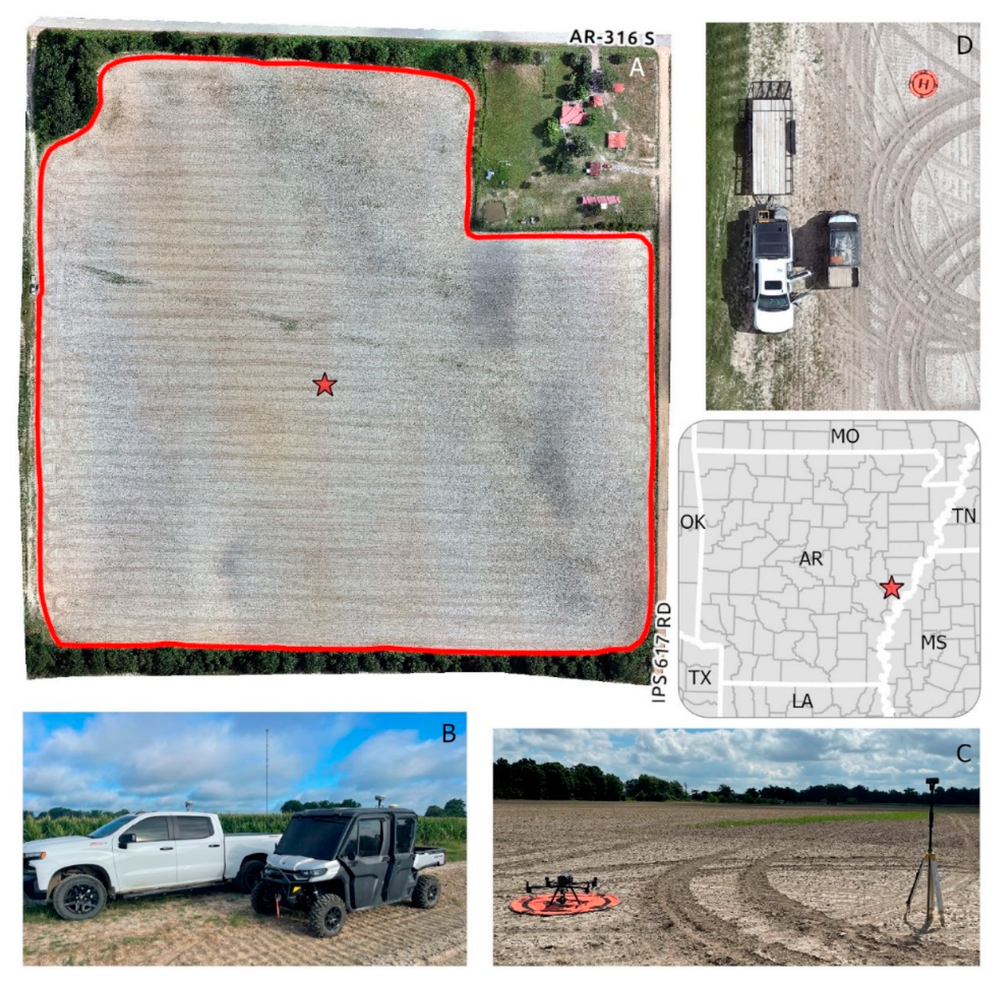
The study site is a 14 ha field in Phillips County, Arkansas (Figure 1). The soil is characterized as a Foley Silt Loam (100%) that is moderately to poorly drained [32]. Phillips County is designated by the state as part of the Cache Critical Groundwater Area for the Mississippi River Valley Alluvial Aquifer in 2015 [3].

2.2. Data Collection

Both ground and aerial surveying were performed on 2 July 2022. The field was tilled in the weeks before the survey, the soil was dry with no standing water, and no vegetation was present. The winds were mostly from the south at 5 m s⁻¹. The sky was mostly clear, temperatures were warm, ranging from 28 to 30 °C, and humidity was relatively high, with dew point temperatures between 23 and 25 °C. Two RTK surveying equipment categories were used for data collection: (a) aerial surveying (sUAS-based photogrammetric system) and (b) agro-terrestrial surveying (ground surveying) involving a fixed base and rover mounted to a utility vehicle.

The aerial survey was performed using a DJI Matrice 300 RTK (manufacturer: DJI, Nanshan District: Shenzhen, China) equipped with a Zenmuse P1 sensor (manufacturer: DJI, Nanshan District: Shenzhen, China). We used a 35 mm lens on a P1 sensor, which is a 45-megapixel resolution camera. Data were collected in a single flight using a flight speed of 12 m s⁻¹, 75% overlap, and a camera angle of 0° (on nadir). The flight altitude was 120 m above the ground level (AGL), resulting in a ground sampling distance of 0.015 m pixel-1. The total flight time was approximately ten minutes.

The DJI Pilot app was used to create the flight route and control the sUAS during flight. The aerial surveying was performed using RTK correction using the Arkansas Department of Transportation-Real Time Network (ARDOT-RTN). During the flight, the RTK connection performed real-time correction of each image, producing geotags for latitude, longitude, and elevation. Consequently, no further post-processing was required due to the real-time corrections. The raw imagery was stitched using Pix4Dmapper photogrammetry software, Version 4.6.4 [33], to produce an orthomosaic raster (Figure 1) and a LiDAR Point Cloud (LAS) file [34]. After post-processing in Pix4D, the elevation surface consisted of 13,698,371 LAS z points, which is ~404 points per m³.

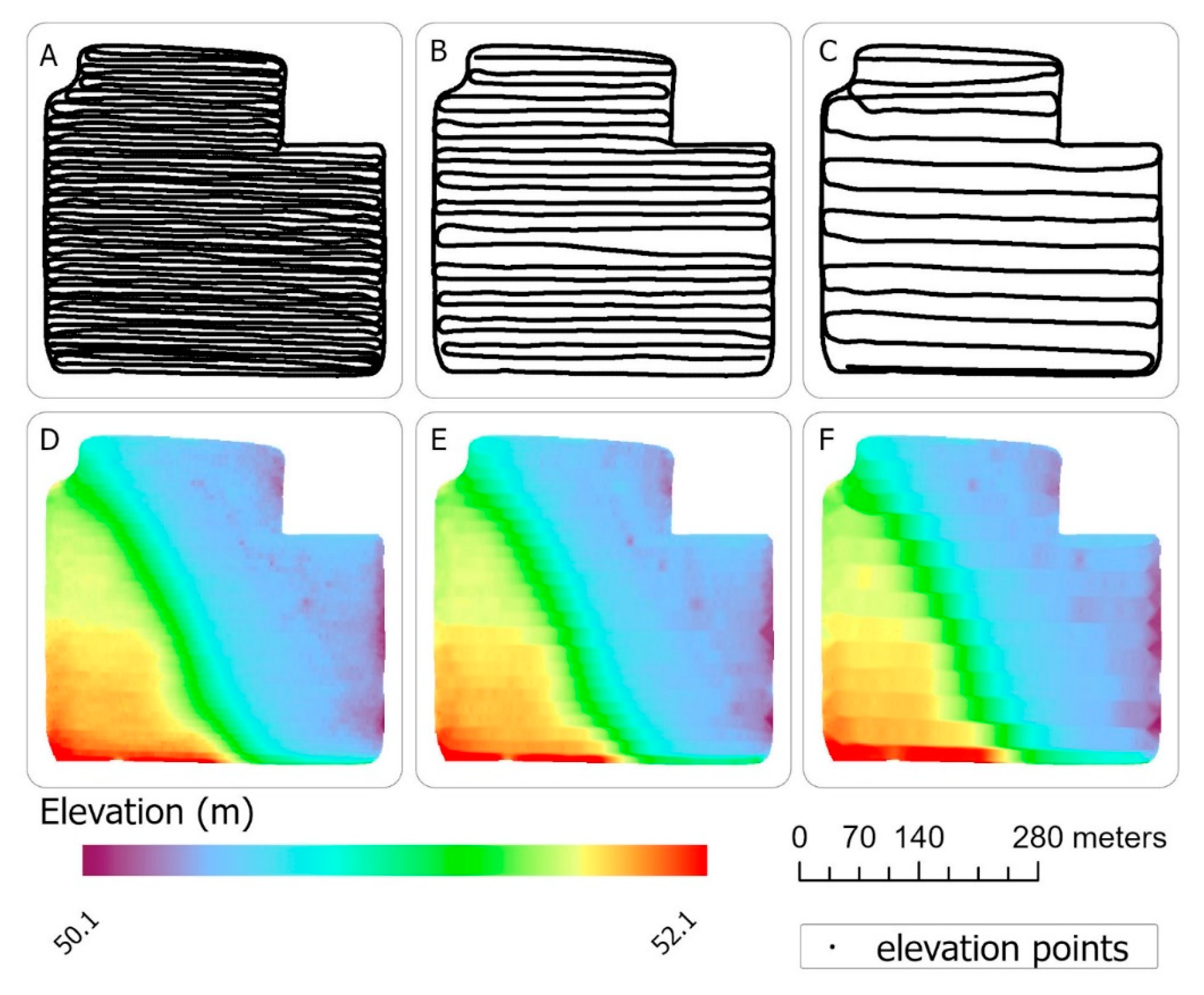
The agro-terrestrial survey was conducted using a 2021 Can-Am Defender Limited Max UTV (Can-Am BRP, Valcourt, QC, Canada) and a Trimble R8s base and rover GNSS receiver (Trimble, Durham, NC, USA). Three separate surveys were conducted at various track spacings (side to side), including 7.62 m, 15.24 m, and 30.48 m. Field elevation was collected every 1.5 m. The purpose of using three spacings was to allow us to evaluate the effect on the interpolation of agro-terrestrial elevation data accuracy. Typical spacings in the region vary between 15.24 m and 30.48 m. The 7.62 m spacing was included to highlight the pros and cons of having large spacing versus narrow spacing, which resulted in two successive doublings of the shortest distance. The R8s and TSC7 process the latitude, longitude, and elevation in real-time and, thus, require no post-processing of the agro-terrestrial data set.

2.3. Data Processing

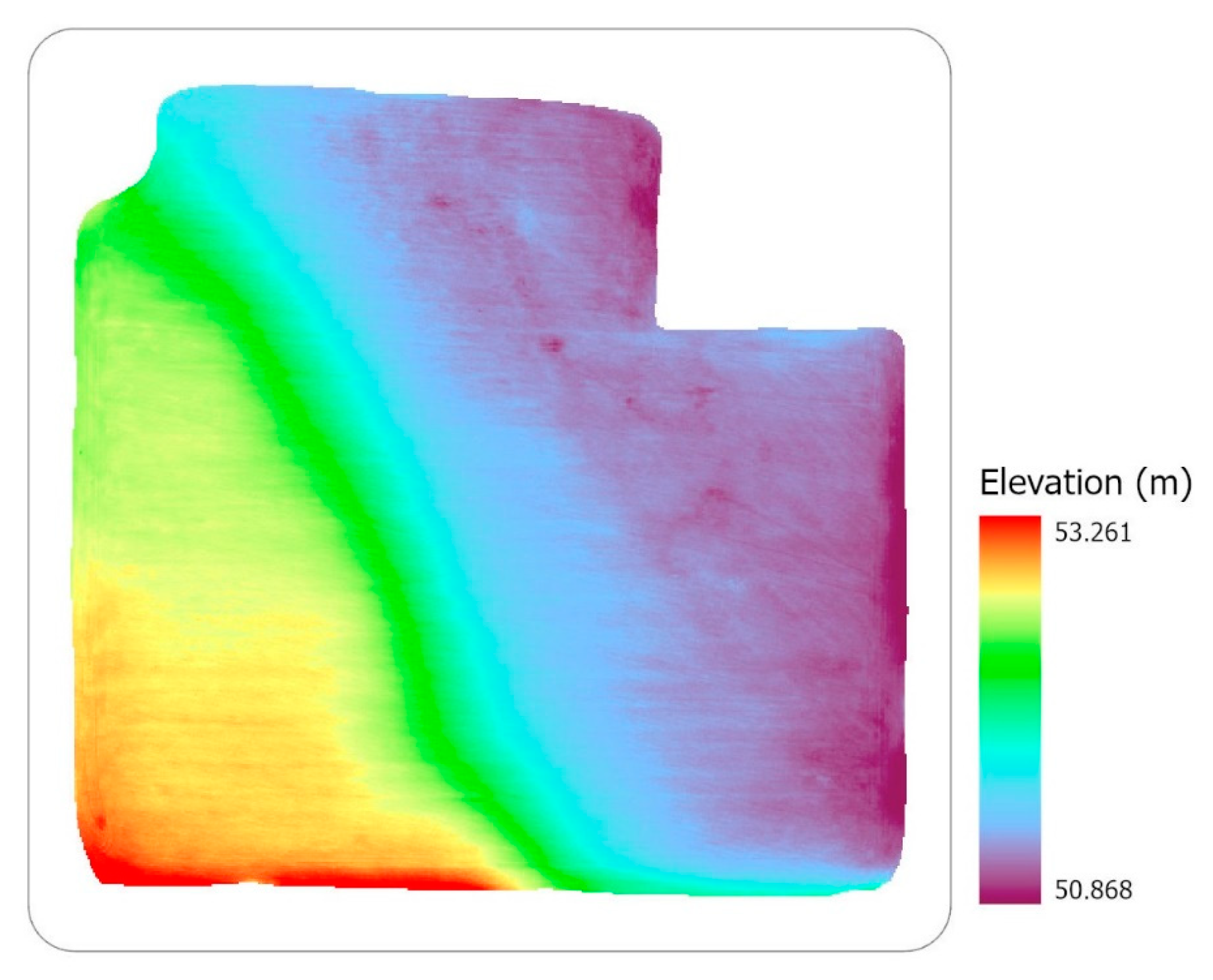
ArcGIS Pro geoprocessing tools [35] were used to clip, extract, interpolate, and visually inspect the elevation data for both survey methods. The inverse distance weighting (IDW) interpolation method was used with both aerial and agro-terrestrial survey data, for generating a one-meter raster-based digital elevation model (DEM). The IDW method determines in-between cell values using a linearly weighted combination of known sample points across a surface [36,37]. After IDW was completed, the surfaces were clipped to the field boundary (Figure 1) to assess the difference between the aerial and ground survey raster datasets generated by the IDW interpolation.

There was an absolute elevation difference between the aerial surveying and agro-terrestrial outputs since the aerial surveying was not corrected using GCPs. To compare the agro-terrestrial survey point elevations with the mean corrected aerial elevation raster for each of the three track spacings, the relative elevation difference between the aerial and ground-based surveys, that is, the means of the two datasets, must be the same. To have a valid comparison between agro-terrestrial and aerial surveying outputs, Equations (1) and (2) were used to adjust the digital elevation of the aerial raster by applying the mean difference between the ground and aerial rasters. This was a required step to assess the relative elevation differences between the two surveying approaches. After the mean difference adjustment, the relative elevation difference was assessed between each individual agro-terrestrial survey data collection point and the raster for the aerial survey.

$$SMD={\mu }_{agro}-{\mu }_{ASE}$$

(1)

$$sUAS=SMD+ASE$$

(2)

where SMD is the elevation difference between the two methods, μ_agro is the mean elevation of the agro-terrestrial survey points, μ_ASE is the mean elevation of the aerial survey raster as extracted by the agro-terrestrial survey points, and sUAS is the set of mean adjusted (corrected) aerial survey surveying values.

The focus of this project is on the relative elevation differences between the two surveying methods. Various factors impact aerial elevation accuracy, including flight altitude, sky condition (clear vs. cloud), terrain type, topography, ground control points, onboard GNSS system, and camera quality [38]. Absolute and relative errors were calculated to assess aerial elevation accuracy. Five statistical parameters were assessed: absolute and relative root mean square error RMSE (Equation (3)), mean bias error MBE (Equation (4)), percent root mean square error %RMSE (Equation (5)), percent mean bias error %MBE (Equation (6)), and percent bias P_BIAS (Equation (7)) [39,40]. The absolute RMSE and MBE were reported to assess the absolute elevation differences between the two surveying methods without using GCPs.

$$RMSE=\sqrt{\frac{{\sum }_{i=1}^n{({agro}_i-{sUAS}_i)}^2}{n}}$$

(3)

where agro is the ith agro-terrestrial elevation value, sUAS is the ith mean adjusted aerial elevation value, and N is the total number of observations.

$$MBE=\frac{1}{n}\sum _1^n(Z_{agro}-Z_{sUAS})$$

(4)

where Z_agro is the ith agro-terrestrial elevation value, Z_sUAS is the ith adjusted aerial elevation value, and n is the total number of observations.

$$\mathrm{\%}RMSE=\frac{RMSE}{{\overline{x}}_{agro}}\times 100$$

(5)

where $\overline{x}$_agro is the mean of measured agro-terrestrial elevation values.

$$\mathrm{\%}MBE=\frac{MBE}{{\overline{x}}_{agro}}\times 100$$

(6)

where $\overline{x}$_agro is the mean of measured agro-terrestrial elevation values.

$$P_{BIAS}=\left[\frac{{\sum }_1^n\left(Z_{agro}^{obs}-Z_{sUAS}^{sim}\right)\times 100}{{\sum }_1^n{Z}_{agro}^{obs}}\right]$$

(7)

where $Z_{agro}^{obs}$ is the average agro-terrestrially measured elevation value during the simulation period and $Z_{sUAS}^{sim}$ is the average adjusted (simulated) aerial elevation value during the simulation period.

2.4. Time Efficiency Comparison

The agro-terrestrial survey data are time-stamped to the nearest second for each point collected with the R8s Trimble receiver. Since the R8s and TSC7 process the latitude, longitude, and elevation in real-time, there is no post-processing needed for the agro-terrestrial dataset. The aerial survey method’s collection time is recorded using the time stamps on the images; processing time includes the time it takes to stitch the images into a single orthorectified surface, including extracting elevations from the photogrammetry process. Only the collection and processing times were compared for the efficiency assessments made between the two methods.

2.5. Survey Equipment Cost Comparison

The estimated equipment cost comparisons were based on the cost of the equipment in July 2023. There are direct and indirect costs associated with each of the survey methods. Direct costs include the capital costs for procuring equipment, while indirect costs might include data collection, data processing time, and travel to and from a job site. Labor or travel costs to and from site were not included, as they would be similar for both methods.

The raster comparison assessment compared the interpolated surfaces of the agro-terrestrial survey to the aerial interpolated elevation surfaces. The statistical parameters were utilized to quantify the statistical differences between the aerial and ground-based datasets at ground-based points. In order to visualize those differences, elevation raster maps were generated from the surface-based points for each of the three spacings. Using the raster generated from the aerial survey and the three rasters generated by the three spacings of the agro-terrestrial survey, map algebra [41] was used to assess the spatial distribution of the differences in elevation. The differences between each of these three ground-based rasters and the aerial raster were calculated and mean-corrected using the ArcGIS Pro Raster Calculator tool (ESRI, Redlands, CA, USA).

It was observed that the UTV sank into the soil as it moved across the field. In order to quantify the possible effect that the tire track may have had on the SMD, the depth of the tire track was analyzed. In ArcGIS Pro, the orthomosaic was imported, and two lines were created that followed one of the tire tracks east-west across the width of the 465 m field. Along those two lines, 125 points were generated, and elevations were extracted from the aerial raster and recorded at each point. The mean elevations from the points on the track were then subtracted from those between the tracks. This number can be considered the error along that track caused by the depth of the tire track.

Finally, the aerial elevation surfaces were compared to the national standard elevation dataset (3DEP), a one-meter DEM [42] generated from a LiDAR collected at the study site in 2014 [43]. The metadata for the LiDAR collection that the DEM was produced from state that the raw accuracy is 0.088 m RMSE z, 0.172 m 95% [44]. This analysis allowed for the comparison of the aerial survey method to a government-maintained (authoritative) elevation dataset that is external to this study and widely distributed. The aerial raster was subtracted from the 3DEP DEM using the ArcGIS Pro Raster Calculator tool.

3. Results

3.1. Aerial Surveying vs. Agro-Terrestrial Surveying

The aerial survey data collection was completed in a single flight (~10 min), and the processing time for quarter resolution was ~14 min (stitching time), resulting in ~0.59 points per m². The resulting one-meter aerial raster is shown in Figure 2. The spatial pattern of elevation reveals that the highest elevations are along the western half of the southwestern border, and lower elevations trend diagonally across the field toward the northeast. The UTV paths cross the field mostly in the east-west direction (Figure 3A–C).

The three SMD differences between the aerial raster and the three lateral spacings of the ground-based survey range were slightly greater and less than zero (

Table 4. Comparison of survey method differences (SMD) for two survey methods and three survey spacings for a commercial rice field in NE Arkansas.

Spacing (m)	SMD (m)	Differences in SMD	N
7.62	−0.8135	−0.00007	9198
15.24	−0.8124	−0.00117	4283
30.48	−0.8148	0.00123	2632
	Mean SMD (m)	Mean difference (m)	Total n
	−0.81342	−0.00000333	16113

). A total of 9198, 4283, and 2632 points were generated for the 7.62 m, 15.24 m, and 30.48 m surveys, respectively. The reported SMDs were all approximately −0.81 m. The mean SMD was −0.81 m (Table 4).

For the 7.62 m, 15.24 m, and 30.48 m agro-terrestrial surveys, the aerial survey achieved relative RMSE values of 0.0147 m, 0.0160 m, and 0.0315 m and Rel%RMSE values of 0.0288 m, 0.0313 m, and 0.0315 m. For the ground-based surveys, the closest survey spacing produced the lowest RMSE of 0.0147 m (

Table 5. Statistical parameters used in comparing three ground survey spacings to an aerial survey method.

Spacing (m)	N	Rel RMSE (m)	Rel RMSE (%)	MBE (m)	MBE (%)	PBIAS (%)
7.62	9198	0.0147	0.0288	−0.4872	−0.9588	−1.6056
15.24	4283	0.0160	0.0313	−0.8124	−1.5986	−1.5993
30.48	2632	0.0161	0.0315	−0.8147	−1.6032	−1.6034

). The aerial survey was within the ASPRS NVA 95th percentile [28] when compared to all three ground-based survey spacings.

Descriptive statistics were calculated for the three ground surveying spacings. Plotting the three ground survey spacings and the aerial survey showed relatively the same accuracy between the methods (Figure 4). The descriptive statistics results showed a consistent pattern with slope and intercept values within the same range between the three surveying distances. The descriptive statistics reveal the exceptionally small variability in these differences of < 0.3 mm.

3.2. Time Efficiency Comparison

Across three agro-terrestrial lateral spacings, the smaller the spacing distance, the longer the data collection time. The agro-terrestrial survey collection time at 30.50 m, 15.24 m, and 7.62 m spacing was ~11, ~18, and ~38 min, respectively. In other words, the 7.62 m spacing took fourfold more time than the 30.5 m spacing. There was no processing time beyond removing the points from the TSC7 Trimble controller.

The aerial survey was conducted on a single 11 min 21 s flight. The processing time depends on the computational capabilities (processor and memory RAM) and the end users’ selected options while setting up the Pix4D project parameters. For example, at full, half, and quarter resolution, the system can process 28.9, 6.8, and 0.59 points m⁻², respectively. At full resolution processing, the stitching process required 598 min, almost 60 times longer than the collection time of the 30.50 m spacing with the agro-terrestrial surveying (

Table 6. Time efficiency comparisons in collection and processing between agro-terrestrial and aerial surveys in minutes as well as computer processing capabilities for photogrammetry.

Study Site	Collection Time (min)	Processing Time (min)	Total Time (min)	Time Difference from 7.62 m Agro-Terrestrial (min) *	Elevation Point Density (per m2)	CPU Cores
Agro-terrestrial 30.50 m	11	0.00	11	NA §	NA	NA
Agro-terrestrial 15.25 m	18	0.00	18	NA	NA	NA
Agro-terrestrial 7.62 m	38	0.00	38	NA	NA	NA
M300 full resolution	10	598	608	+570	28.9	6
M300 half resolution	10	136	146	+108	6.8	6
M300 quarter resolution	10	14	24	−14	0.59	6

* A positive number indicates more time is required to collect survey data, and a negative number indicates less time is required to collect data. ^§ Not applicable.

). However, the quarter-resolution processing of the aerial survey required approximately 24 min, which is 14 min faster than the 7.62 m agro-terrestrial survey (38 min). Additionally, processing can occur while other tasks are being performed. Hence, the time used during post-processing is autonomous and does not require human attention while running.

3.3. Survey Equipment Cost Comparison

The equipment costs are summarized in

Table 7. Cost comparisons between agro-terrestrial and aerial survey equipment.

Agro-Terrestrial Equipment	Cost Before Taxes
UTV with trailer	$40,000
John Deere RTK Base/Rover/T3RRA Cutta	$40,000
Total	$80,000
Aerial Equipment
M300 RTK Equipment Bundle	$29,199
Total	$29,199

. The aerial equipment is substantially less expensive than the agro-terrestrial equipment. We did not include the cost of the PC in the equipment cost for the UAV methods. The analysis described can be done with a high-quality laptop with at least 32 GB of RAM and 1 TB of hard drive space. The authors assume that in the contemporary era, it is expected that farming operations using UAVs or even ground-based surveying techniques will have access to an appropriate computer. There are also operating expenses not covered in the estimates, such as fuel and labor, both of which vary with time and location. Both methods require the surveyor to travel to the site, but it should be acknowledged that pulling the UTV behind a pickup truck would cost more than not needing a trailer. Also, the fuel capacity of the UTV is 40 L, the U.S. national average price of fuel was $4.27 on 2 July 2022, and the UTV used less than a tank of gas to drive all three ground survey widths. This cost is therefore estimated at <$40 per collection for the relatively flat 14 ha field.

4. Discussion

This study assessed the use and accuracy of RTK sUAS for aerial topographic surveying compared to ground surveying. Its significant contribution is demonstrating that commercial-grade RTK sUAS was able to collect elevation data with high accuracy, precision, and greater efficiency than traditional agro-terrestrial methods, given the appropriate field conditions and weather. Additionally, the relative accuracy of RTK sUAS as determined using statistical evaluations is within the reported accuracy of others [27,42].

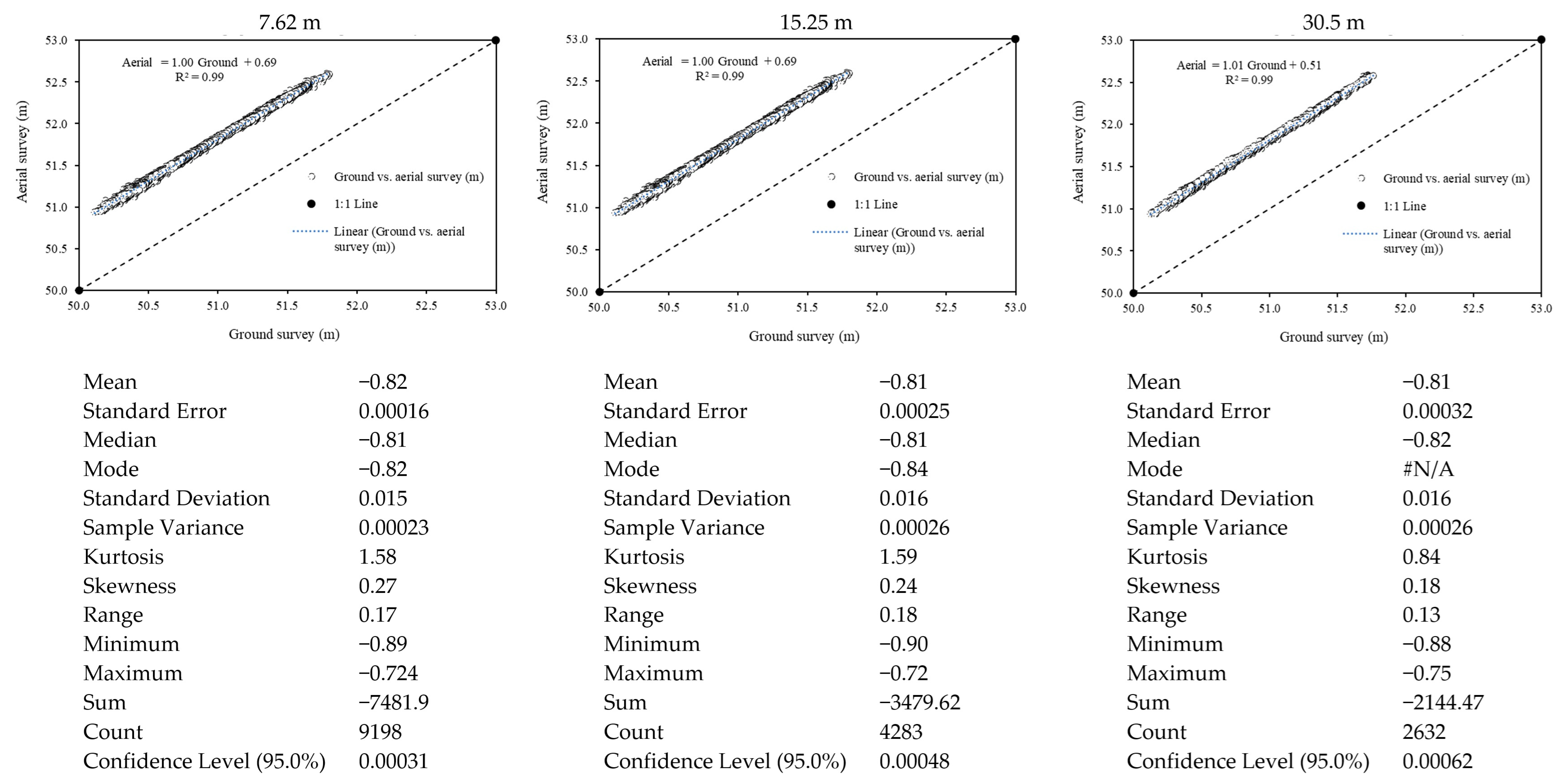
In this study, aerial surveying had an average relative vertical elevation accuracy RMSE of 0.015 m across three different datasets totaling 16,113 sample points. Rabah et al. [27] reported vertical RMSE absolute accuracy between 0.026 m and 0.029 m. A significant finding related to the aerial surveying in this study compared to the previous aerial studies was to demonstrate the impact of GSD on the RMSE. The reported GSD in Taddia et al. [45] and Rabah et al. [27] studies were 0.006 and 0.026 m per pixel, respectively. Similarly, this aerial survey was completed with a 45-megapixel camera, flown at 120 m altitude AGL, resulting in a GSD of 0.015 m and achieving a relative RMSE of 0.015 m. These results indicate that advances in camera technology (i.e., resolution, focal length, etc.) can reduce the relative RMSE and, thus, increase surveying accuracy.

Current literature that evaluates RTK sUAS elevation accuracy uses GNSS equipment. However, these were oftentimes not correcting the position of the RTK sUAS during flight to collect elevations on ground targets used to check or correct the images during bundle block adjustment of the photogrammetry process. Using the direct georeferencing method on RTK-sUAS often achieves an RMSE z of 0.035–0.18 m when using control points or GCPs with absolute accuracy [46,47,48]. However, these accuracies and standards are not applicable when conducting a field-scale agriculture survey, since agriculture purposes only require local or relative elevation changes to implement agriculture practices in any given field. Oftentimes, like laser-controlled equipment, a GNSS base station is set up in an unknown location and controls a rover for collecting elevation, physically marking the ground for levee irrigation, or controlling grading equipment to bring a field to a particular slope for increasing irrigation efficiency. Furthermore, in terms of collecting elevation, agriculture surveyors will collect elevations referenced to a local grid to track elevation change throughout an agriculture field. While absolute elevation is not, therefore, the goal of RTK precision for agricultural elevations, there is value in the consistency between surrounding elevation readings and local agreement between surveyed surfaces and the ground surface. This is the realm of relative elevation accuracy.

Absolute errors were not used in this study due to differences between the datums used by the different methods and the spatial-temporal variability of making elevation readings with different equipment at different times. The purpose of the relative elevation method is to show that surveyors do not need to use GCPs when performing agricultural operations. Relative errors, on the other hand, provide valuable evaluation metrics to quantify vertical estimation uncertainties. There are many factors that can contribute to the error between a ground-collected surface and an aerial-collected surface [49], including, but not limited to, equipment quality, multipath errors, altitude of the aerial collector, resolution of the camera, wind speed, clarity of the air, etc. In our study, the RMSE ranged between 0.0147 and 0.0369 m. The PBIAS values ranged from −1.6 to 2.09%, indicating that some fields’ elevation values were higher than the actual elevation and others were lower than the measured elevation values. Based on the P-bias, the UAS surveying produces an acceptable elevation estimation compared to the measured elevation using ground surveying, where the PBIAS ranges are always recommended at ~±10% [50]. The MBE and %MBE were satisfactory and provided more insight into the error’s directions.

Based on this study’s findings, the aerial surveying methods produced a more precise and detailed surface elevation raster than the ground surveying methods. Ground surveying techniques need a path spacing of less than 7.62 m to approach the same precision as the aerial survey. In addition, the ground survey required approximately 40 min to define the topography of the 14 ha study field. Conversely, aerial surveying proved significantly more efficient by collecting imagery in ~10 min and processing a quarter-resolution elevation raster (0.56 points per m²) in ~14 min. However, in the ~14 min processing window, other tasks can be performed, so this time can be shared with other operations.

Aerial surveying would be expected to become increasingly efficient as the field area increases. The combination of advances in technology and regulations suggests even more potential efficiency in the future. For example, as RTK UAS-based cameras improve from 45 MP to 100 MP and flying ceilings increase from 120 to 240 m, it would increase the coverage area by more than fourfold. This would require FAA regulation changes to the maximum allowable ceiling for sUAS without a waiver.

Ground surveying requires an RTK-GNSS base, rover setup time, and a basic understanding of the controller (display) used to set up the receivers and data collection. However, aerial surveying requires these same skills, plus experience in coordinate systems, datums, photogrammetric software, GIS, computer hardware capabilities, an FAA Part 107 Drone Pilot certification, and an understanding of airspace regulations.

There are also advantages and disadvantages to the aerial and agro-terrestrial survey methods relating to current weather and soil moisture conditions. Weather conditions impact each method differently. It is best to perform both methods in clear skies for optimal RTK-GNSS operation. In wet soil conditions, the aerial survey method has a clear advantage because a ground survey method should not be completed if the field is too wet due to the risk of the UTV getting stuck and rutting up the field. Unfortunately, aerial imagery is best collected in clear-sky daytime conditions, while ground survey methods are not impeded by low-light conditions and can even be performed comfortably at night.

Other advantages and disadvantages of ground-based surveying vs. aerial surveying are summarized in

Table 8. Advantages and disadvantages of ground-based surveying vs. aerial surveying with an sUAS.

Method	Advantages	Disadvantages
Ground surveying	Widely adopted Technologically simple Requires less technical expertise High accuracy with ground vegetation Low processing time Can survey at night	Long collection time More expensive Cannot survey if the ground is wet Error related to soil compression by the survey vehicle and elevation averaging between tires of a four-wheel vehicle. Data are in point format, not in raster format
Aerial photogrammetric surveying	Low collection time Less expensive Can survey if the ground is wet More precise	Ground vegetation impacts accuracy Requires UAS certifications Requires more technical expertise Cannot survey at night

.

The fact that the UTV sank almost 1 cm into the soil as it traversed the field hints at another way the aerial method is more accurate than the agro-terrestrial method, as the sUAS does not require any contact with the soil. Thus, there is no rutting or compaction. Soil textural properties, soil moisture, and field condition are all factors that would be expected to modify the compressibility of the soil, adding variability to how this would differ between fields. It is also notable that when the UTV is traversing the field, the rover antenna is sampling the average elevation between the four tires that are in contact with the ground. The sUAS, on the other hand, have the ability to estimate elevations at many points per meter, suggesting it is better at accuracy and precision when characterizing undulations of the field. For precision grading, there are limited returns when working with elevations at XY submeter resolutions in flat terrain. This is because the implement used for moving the soil, a dirt pan or bulldozer, tends to be wider than three meters. So, while the aerial method might be superior in characterizing elevations across the field, there might be no practical benefit.

Even though aerial surveying requires more skilled and knowledgeable operators, this should not deter early adopters from utilizing both surveying methods. The size of the field, or close grouping of fields, is a factor in choosing the best method. For instance, if the field is large (i.e., over 200 ha), it could be more efficient to use aerial methods, which might take ~two hours to collect the data. By comparison, the ground survey technique could require one to two complete workdays to collect the elevation data for the same field, with significantly fewer elevation data points collected owing to the required increased path spacing.

Aerial surveying must comply with FAA regulations and airspace considerations. Most agricultural fields are not in a controlled airspace, which means that no prior approval is necessary to conduct the flight. However, it is always good practice for drone operators to check the airspace and clear any FAA requirements that may be needed.

The M300-RTK (DJI) package price was $29,199 (Table 7), including the UAS, sensors, and flight application software−DJI Pilot 2 (July 2023 USD). At $80,000, the UTV is the most expensive item in the ground surveying equipment setup (Table 7). The equipment costs differed substantially between the two methods. The agro-terrestrial equipment costs were more than double the aerial equipment costs. This affirms that the RTK sUAS method is affordable.

Another issue relates to 2023 Arkansas Legislation, Act 525, which limits the purchase of Chinese sUAS using state funds [51]. This could be the beginning of more stringent regulations for private industry. If that occurs, the value proposition will need to be reassessed, as many similar American and European sUAS are more than double the cost of Chinese manufacturers.

Another potential source of elevation data, which might be a good subject for future consideration, is the elevation data provided by typical harvest equipment. For instance, when a combine traverses a field during harvest, the yield information is attached to yield points, which record elevations and other data. If the elevations from the harvest points were as accurate as the agro-terrestrial methods provided in this research, they might represent a more efficient dataset that already exists for many fields.

This study utilized a single flight along with three different ground surveys conducted all on one day. There was a high number of LAS points (13,698,371 points, which is 404 points per m³) that were generated from 893 aerial images with an overlap of 75% front to back and 75% side to side. These were compared to the three separate sets of ground survey methods, which produced thousands of points each (n = 9189 at 7.62 m spacing, n = 4283 at 15.25 m spacing, and n = 2632 at 30.5 m spacing). One of the shortcomings of this methodology is that the validity and reliability of the correlation between aerial and ground survey methods might be better established by many replications. For the purpose of comparing the two types of methods, the large sample counts of the aerial method are statistically valid, but it will be imperative in future research to establish the repeatability of this aerial method under a variety of conditions. In our future research in the LMRB, we think the best periods to collect this data are the last two weeks in March through the first two weeks in May. While it might be possible, as in this research, that a field not in normal production becomes available outside of this window, this is the typical period when fields are clear of vegetation and ground/aerial surveys can be conducted before planting. After this period, it is more difficult to enter the fields with equipment.

5. Conclusions

The purpose of this study was to assess the relative elevation accuracy of aerial surveying and validate its performance against ground surveying methods. The research results document that aerial surveying was able to accurately generate a digital surface model of an agriculture field more efficiently, precisely, and cost-effectively than agro-terrestrial survey methods, given the appropriate field conditions. The aerial surveying had a relative RMSE of 0.030 m at the 95th percentile when compared to agro-terrestrial surveying, all while adhering to ASPRS standards of quality [28]. This leads to the conclusion that, as it relates to relative elevation, RTK sUAS aerial surveying can be utilized to conduct agricultural surveys without deploying GCPs while adhering to ASPRS quality standards.

As sUAS technology and regulations improve, using higher-resolution cameras that can be flown at higher speeds and elevations will increase the image resolution (i.e., reduce the GSD) and decrease data collection time. The combination of an increase in GSD coupled with longer sUAS battery life would be optimal to cover much larger fields in even shorter times. This would improve the relative accuracy of the RTK survey data for agriculture and further reduce the cost of aerial surveying compared to ground-based surveying. Theoretically, under such conditions, an RTK sUAS could survey hundreds of hectares a day, enabling an agricultural surveyor to expand the available area to survey far more efficiently than current agro-terrestrial methods. Additionally, the survey could be conducted without potential time delays related to field conditions that could limit physical entry to the cultivated portion of the field.

In addition to increasing the capabilities of RTK sUAS, an RTK sUAS equipped with LiDAR could further expand agriculture’s capabilities, with much higher surveying accuracy in light to moderate vegetation fields. The sUAS LiDAR payloads are becoming less costly (less than $50,000 based on 2022 US dollar prices). This could provide a more efficient method of collecting and processing surface elevation data. However, sUAS LiDAR payloads that can achieve similar accuracies found in high-megapixel cameras like those used in this study ($5000–$10,000) are expensive (greater than $100,000). Until these payloads become as accurate and cost-effective as photogrammetric methods using cameras, they will not be as cost-effective as RTK sUAS photogrammetry or traditional agro-terrestrial survey methods.

With advances in agriculture surveying data collection and processing, coupled with the appropriate guidance control systems on agriculture equipment, early adopters could enhance farming operations and increase operational efficiency. Aerial surveying could have a wide variety of applications, including but not limited to field leveling, rice paddy preparation, irrigation design, and drainage system design, among other precision agriculture applications. Currently, there is no capability to define large-scale farmland topography accurately and efficiently. Precisely defining the topography of an agricultural field only enhances the precision of precision agriculture. In meeting the goals of precision agriculture, sUAS-based agricultural surveying advances the goal of increasing agricultural production, optimizing outputs, reducing inputs, and increasing sustainability and resilience for farmers worldwide.