Trajectory Planning and Control Design for Aerial Autonomous Recovery of a Quadrotor

Abstract

One of the most essential approaches to expanding the capabilities of autonomous systems is through collaborative operation. A separated lift and thrust vertical takeoff and landing mother unmanned aerial vehicle (UAV) and a quadrotor child UAV are used in this study for an autonomous recovery mission in an aerial child–mother unmanned system. We investigate the model predictive control (MPC) trajectory generator and the nonlinear trajectory tracking controller to solve the landing trajectory planning and high-speed trajectory tracking control problems of the child UAV in autonomous recovery missions. On this basis, the estimation of the mother UAV movement state is introduced and the autonomous recovery control framework is formed. The suggested control system framework in this research is validated using software-in-the-loop simulation. The simulation results show that the framework can not only direct the child UAV to complete the autonomous recovery while the mother UAV is hovering but also keep the child UAV tracking the recovery platform at a speed of at least 11 m/s while also guiding the child UAV to a safe landing.

1. Introduction

Unmanned systems have gradually demonstrated their powerful functions in industrial, rescue, and consumer fields over the last few years [1]. As a result, one of the primary concerns of researchers is the autonomous operation capability of unmanned systems. Unmanned systems with autonomous operation capability can frequently perform more tasks in complex environments, effectively improving relevant practitioners’ work efficiency and reducing work risks. However, in addition to the complexity of people’s work tasks, a single unmanned system is frequently limited by its size and load capacity, rendering it incapable of completing increasingly complex tasks on its own. Therefore, using unmanned systems to collaborate can effectively broaden the scope and capabilities of unmanned systems, enrich the work of unmanned system scenarios, and provide unmanned systems with broader application prospects.

Child–mother unmanned systems are currently receiving a lot of attention in the cooperative operation of unmanned systems because of their ability to effectively extend the operational range and time of child unmanned systems, reduce the operational risk of mother unmanned systems, and improve the mission flexibility of unmanned systems. At the moment, the most common child unmanned systems use an unmanned surface vessel (USV)/unmanned ground vehicle (UGV) as the mother system or mother platform, and a multi-rotor unmanned aerial vehicle (UAV) as the child system [2,3,4,5], with a lot of research focusing on the aerial child system’s recovery and landing. These studies laid the groundwork for autonomous cooperative operation of aerial platforms and ground or surface platforms. However, due to terrain and environmental factors, ground and surface platforms cannot always meet the recovery needs of multi-rotor UAVs. To address this issue, we propose an unmanned child–mother system that includes a separated lift and thrust vertical takeoff and landing (VTOL) UAV as the mother UAV and a multi-rotor UAV as the child UAV. The system can effectively integrate the benefits and characteristics of both platforms while reducing the impact of the environment and terrain on the recovery and release of the child UAV. Therefore, research into the autonomous landing and recovery of aerial moving platforms can add to the composition of the child–mother unmanned system and promote the development of unmanned system cooperative operation.

1.1. Related Work

An accurate and low-cost localization method is critical for the autonomous landing of multi-rotor UAVs on ground and water platforms. AprilTag, a visual reference system proposed in 2011, has better localization accuracy and robustness than visual localization systems such as ARToolkit and ARTag [6,7,8]. With better localization accuracy and robustness, it is now widely used in robot localization, camera calibration, and augmented reality, among other applications. The system can identify and localize specific tags on targets, provides relative camera position information quickly and accurately using monocular cameras, and has been widely used in UAV navigation and localization. Nanjing University researchers proposed a “T”-shaped cooperative tag in 2013 and improved the pose calculation method based on feature points. However, the algorithm’s real-time performance need to be improved [9]. In 2018, a tag set comprising a monocular camera and AprilTag is used in conjunction with Kalman filtering to achieve UAV localization in an indoor GPS signal rejection environment, and the feasibility of the localization scheme is demonstrated through indoor flight experiments [10]. Furthermore, the researchers used GPS localization in conjunction with cooperative tag-based visual localization to achieve long-term deployment and autonomous charging of UAVs outside, and the designed positioning scheme demonstrated good autonomous landing accuracy [11]. The recovery mission was divided into stages based on relative distance, with GPS positioning used in the long-distance approach phase and more accurate visual positioning used in the close landing phase, allowing the UAV to land precisely on the moving surface platform [2]. The combination of visual positioning and model predictive control (MPC) could also be used to control the quadrotor landing on the moving platform; however, the movement speed of the platform is slow and the motion state is rather simple [12].

Because of the platform’s slow motion speed and relatively simple motion state, the control method of position point tracking in the preceding studies can meet the control requirements of autonomous landing. However, as the landing platform’s motion speed increases and the motion state becomes more complex, the corresponding trajectory planning algorithm must be designed to generate a smooth landing trajectory and guide the accurate landing of child UAV on the moving platform.

To generate perching trajectories for a small quadrotor perched on tilted moving platforms, geometric constrained trajectory optimization is used [13]. Furthermore, MPC can be used to generate landing trajectories. When faced with the trajectory planning problem of autonomous landing point-to-point, MPC is used to generate a smooth motion trajectory from the multi-rotor UAV to the recovery platform, as well as to reduce the relative distance, and the real-time motion trajectory can be generated using the variable prediction step [14] or variable time step [5] method. The motion trajectory can also be used as input to MPC. A smooth landing trajectory is generated by estimating the motion trajectory of the moving platform and using the estimated trajectory as input to the MPC trajectory planner to guide the UAV to land accurately on the ground platform moving at 15 km/h [15,16].

The current research focuses on the autonomous landing of the surface and ground platform when the movement speed of the multi-rotor UAV facing the platform is low, mostly below 3 m/s [2,3,4,5,13,14,17,18], and the ground platform movement speed is sometimes relatively fast, reaching 4.2 m/s (15 km/h) [15,16,19]. However, the flight speed of the fixed-wing state aerial landing platform far exceeds that in existing research; therefore, this paper has particular significance for further applications for aerial child unmanned systems.

1.2. Contribution

In this paper, we conduct research on the trajectory planning and control of the child UAV during the aerial recovery process, and propose a method suitable for the recovery of the child UAV while the aerial platform is moving at high speeds (11 m/s) or is in a hovering state. Different stages of the recovery mission are established through the division of the air platform’s autonomous landing mission and a visual positioning algorithm based on the Kalman filter is designed to continuously estimate the state of the recovery platform. Furthermore, the kinematic model of the mother UAV is established to estimate the trajectory of the mother UAV and the linear MPC is used to generate the autonomous recovery trajectory. It is worth mentioning that the kinematic model can predict the trajectory of the mother UAV for any period of time. The built visual simulation environment is shown in Figure 1. As a result, the mother platform’s tracking accuracy can be adjusted by adjusting the predicted trajectory input to the MPC trajectory generator, as shown in Figure 2. The child UAV has a relatively fast movement speed in the problem presented in this paper and aerodynamic effects have a greater impact. In reference [17], wind turbulence effects were considered during controller design; however, the methods used for wind speed measurement and turbulence simulation deviate from the real-world conditions of our study. References [2,3,4,5,13,14,15,16,19] do not account for external wind disturbances. To incorporate the influence of aerodynamic characteristics in the child UAV, we adopt the dynamics model with rotor aerodynamic drag proposed in reference [20]. We then integrate this simplified aerodynamic drag into the controller design to mitigate its impact on control accuracy. As a result, a geometric tracking controller is proposed that takes aerodynamic resistance into account, as well as a feedforward operation to meet response speed and precision tracking of high-speed trajectories [20,21]. The method proposed in this paper produced good results in a visual simulation environment and it serves as a useful reference for subsequent actual real-world experiments.

1.3. Problem Definition

In this study, the child UAV is recovered while the mother UAV is in multi-rotor hovering and fixed-wing circling modes, and a landing platform with a visual location tag is mounted above the mother UAV. The child UAV serves as the foundation for the entire recovery and landing mission process. As shown in Figure 3, the distance from the mother UAV is divided into two stages: approaching and landing.

During the approaching stage, the flight controllers of the child and mother UAVs obtain their own positioning data via GPS and IMU. Furthermore, the child UAV obtains the position of the mother UAV through the communication module and rapidly reports to the mother UAV. When the child UAV approaches, the child UAV is expected to maintain a safe vertical distance from the mother UAV in order for the visual sensor to detect the visual localization mark.

The recovery mission enters the landing stage once the visual localization mark is detected. To avoid losing the information from the visual localization tag during the landing stage, the child UAV first keeps track of the position of the mother UAV. After the landing command is given to the child UAV, the child UAV begins to descend slowly while keeping track of the horizontal position of the mother UAV. It descends to the recovery platform after meeting the landing error requirements and turns off the motors to complete the recovery mission. The recovery platform is 2 × 2 m square with depth, and an electromagnet is installed underneath the platform so that the child UAV can be dropped onto the platform and held on the platform by the electromagnet when the error between the center of gravity of the child UAV and the center of the recovery platform in the x–y plane is less than 1 m. We give the error requirements that the landing end should meet based on the size constraints in

Table 1. Error requirements at the end of landing.

Error Direction	Positon Error Limit
x	$\pm 1$ m
y	$\pm 1$ m
z	0.1 m

.

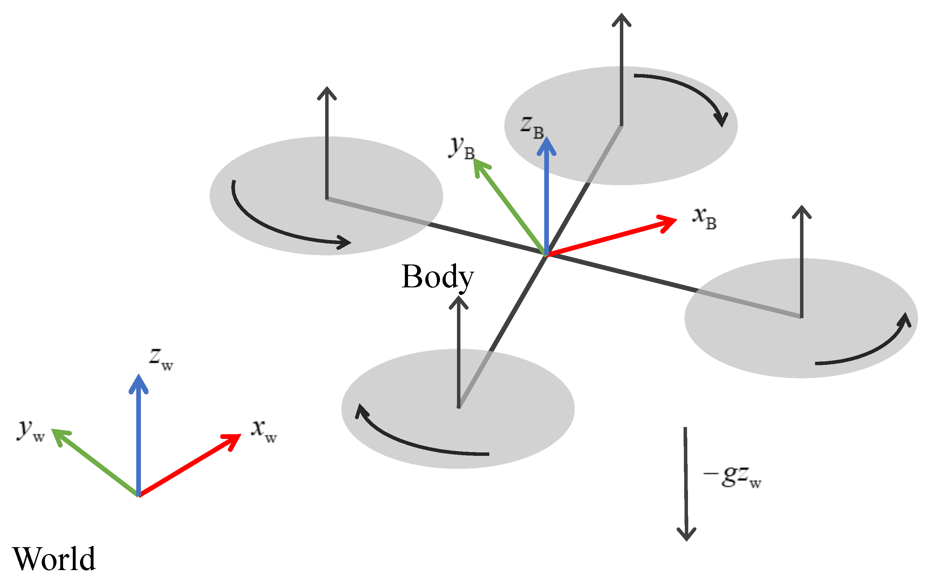
2. Coordinate System Definitions

The child UAV in this paper is a quadrotor, while the mother UAV in the recovery mission is a fixed-wing UAV. In this section, we give the definition of the motion coordinate system of the child–mother UAV, laying the foundation for the subsequent representation of the motion state, force analysis, and algorithm design.

Figure 4 depicts the definition of the coordinate systems. We define the world frame ($O_{\mathrm{w}}{x}_{\mathrm{w}}{y}_{\mathrm{w}}{z}_{\mathrm{w}}$) and the body frame ($O_{\mathrm{B}}{x}_{\mathrm{B}}{y}_{\mathrm{B}}{z}_{\mathrm{B}}$) in the following ways:

1.

Body frame: take the center of mass of the UAV as the origin and the plane of symmetry as the $O_{\mathrm{B}}{x}_{\mathrm{B}}{z}_{\mathrm{B}}$ plane; the $O_{\mathrm{B}}{x}_{\mathrm{B}}$ axis points to the front of the nose, the $O_{\mathrm{B}}{y}_{\mathrm{B}}$ axis is perpendicular to the plane and points to the left side the UAV, and the $O_{\mathrm{B}}{z}_{\mathrm{B}}$ axis points upward, satisfying the right-hand law.

2.

World frame: because $O_{\mathrm{w}}$ is located on the ground at the take-off point of the UAV, the $O_{\mathrm{w}}{z}_{\mathrm{w}}$ axis points upwards perpendicular to the ground, the $O_{\mathrm{w}}{x}_{\mathrm{w}}$ axis points due east, and the $O_{\mathrm{w}}{y}_{\mathrm{w}}$ axis points due north; this coordinate system is commonly known as the East North Up (ENU) coordinate system.

Figure 4. Schematics of the considered quadrotor model with the coordinate systems used.

Figure 4. Schematics of the considered quadrotor model with the coordinate systems used.

We define the position of the center of mass of the child UAV in the world coordinate system, expressed by vector $\mathbf{p}$, and its derivative velocity, acceleration, jerk, and snap are respectively expressed as $\mathbf{v}$, $\mathbf{a}$, $\mathbf{j}$, and $\mathbf{s}$. The center of mass position vector ${\mathbf{p}}_m$ of the mother UAV is also defined in the world coordinate system, and its derivatives are represented by ${\mathbf{v}}_m$, ${\mathbf{a}}_m$, ${\mathbf{j}}_m$, and ${\mathbf{s}}_m$, respectively. In addition, the orthonormal basis $\left\{{\mathbf{x}}_{\mathrm{B}}{\mathbf{y}}_{\mathrm{B}}{\mathbf{z}}_{\mathrm{B}}\right\}$ represents the body frame in the world frame. The orientation of the child UAV is represented as a rotation matrix $\mathbf{R}=\left[\begin{array}{ccc}{\mathbf{x}}_{\mathrm{B}}& {\mathbf{y}}_{\mathrm{B}}& {\mathbf{y}}_{\mathrm{B}}\end{array}\right]$ and its angular velocity $\mathbf{\omega }$ is represented in the body coordinates. The matrix $\mathbf{R}=\left[\begin{array}{ccc}{\mathbf{x}}_{\mathrm{B}}& {\mathbf{y}}_{\mathrm{B}}& {\mathbf{y}}_{\mathrm{B}}\end{array}\right]$ can also represent the rotation from the body frame to the world frame. Finally, we use $\left[\begin{array}{ccc}{\mathbf{x}}_{\mathrm{w}}& {\mathbf{y}}_{\mathrm{w}}& {\mathbf{z}}_{\mathrm{w}}\end{array}\right]$ to represent the three unit vectors in the world coordinate system.

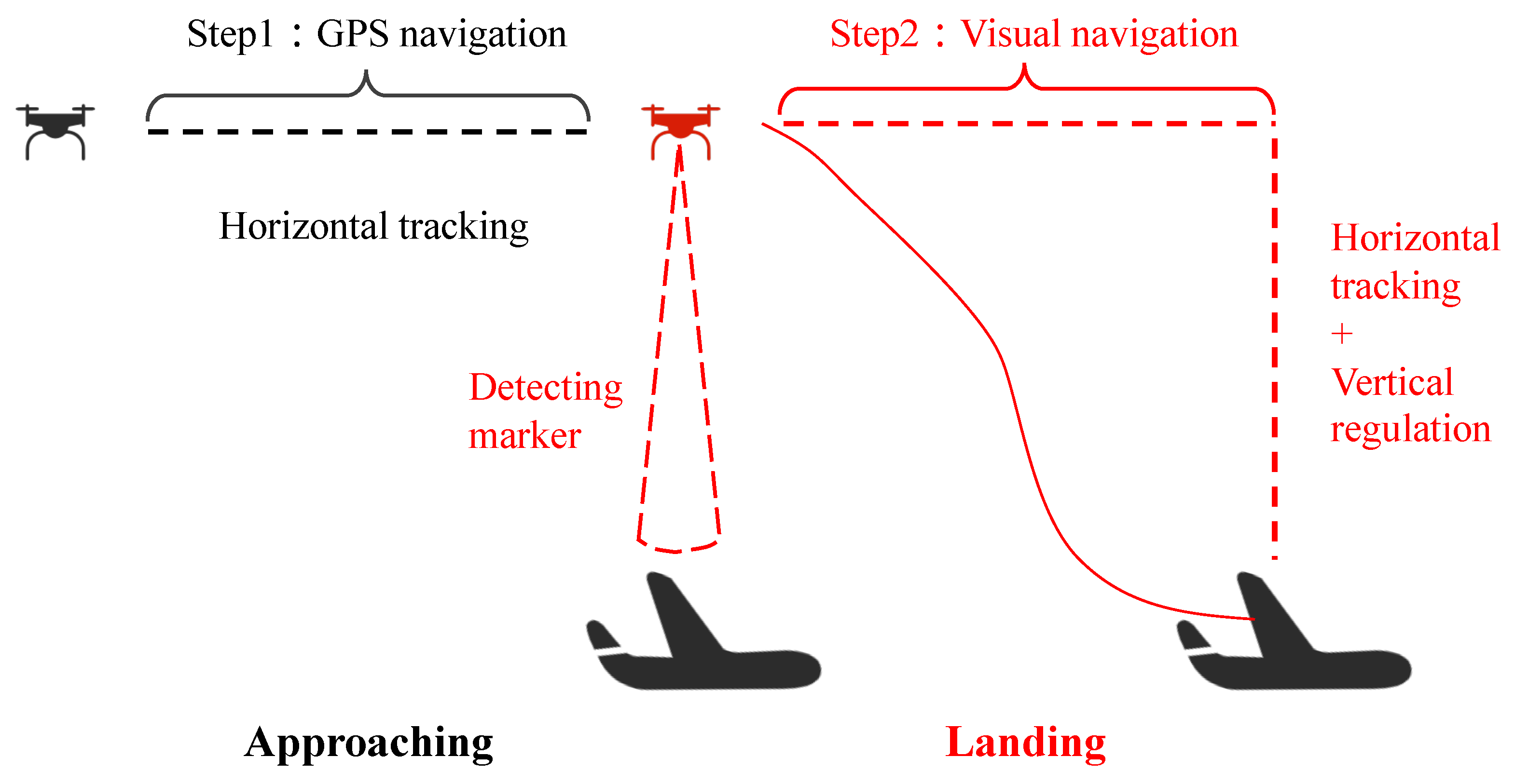
3. Autonomous Landing System

The architecture of the proposed control system, which follows a common multi-layer structure, is shown in Figure 5. The Kalman filter combines visual location information with flight control positioning information from the mother platform to estimate the mother platform’s states and predict the mother platform’s trajectory using a dynamic equation. The MPC trajectory generator receives the predicted trajectory as input and obtains the desired state ${\mathbf{x}}_{\mathbf{D}}$ of the child UAV in the world frame, which is used as the trajectory tracking controller’s input. The angular velocity controller is a cascade control system that receives the expected angular velocity and thrust under the body frame output from the trajectory tracking controller.

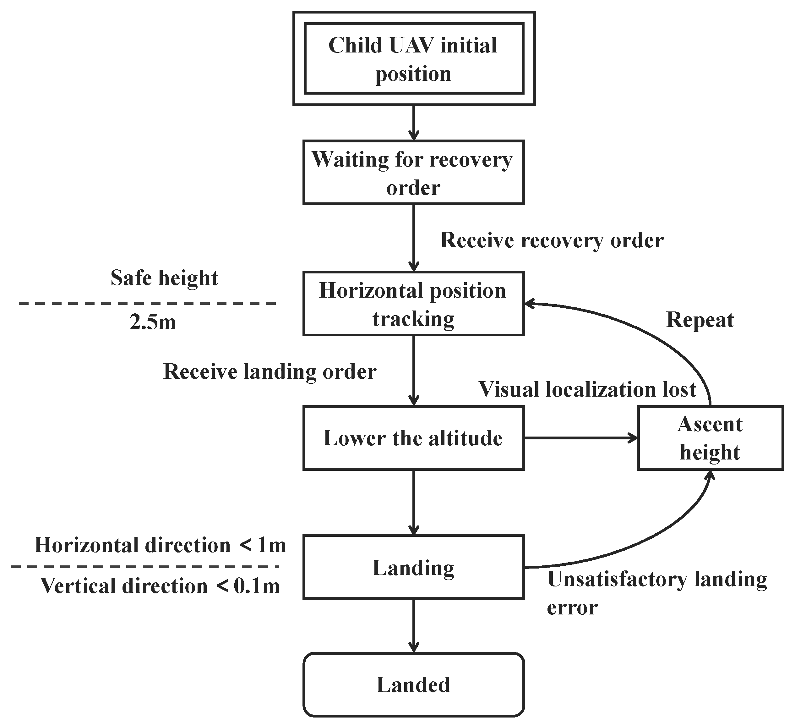
3.1. Landing State Machine

Due to the fast movement of the mother UAV in the autonomous landing mission, the child UAV must have a large attitude angle during flight and visual localization loss is very common. Therefore, we created a landing state machine to control the operating states of the child UAV throughout the recovery process. The state machine handles the mission states of the child UAV, receives mission start and landing commands, and allows the child UAV to rise to the required height for a second landing if visual localization is lost. The control logic of the state machine is shown in Figure 6.

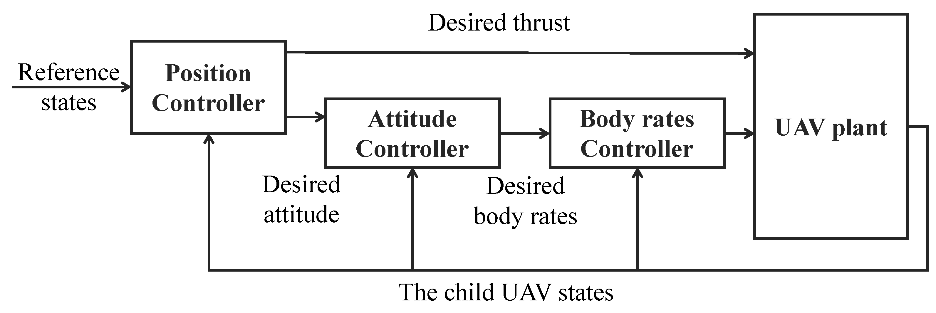
3.2. Angular Velocity Controller

The angular velocity controller is an onboard embedded unit in charge of maintaining the desired body rate $\mathbf{\omega }$. The controller block generates the desired motor speeds and accepts the desired body rate $\mathbf{\omega }$ as well as the normalized throttle value. The PID controller from the Pixhawk 4 flight stack [22] was used in the software-in-the-loop simulation. However, the proposed system is not dependent on the choice of a particular angular velocity controller.

3.3. Nonlinear Trajectory Tracking Controller

The nonlinear $\mathsf{SE}\left(\mathsf{3}\right)$ state feedback trajectory tracking controller is the next step in the pipeline. We chose a quadrotor dynamics model that considers aerodynamic drag of rotors when designing the controller because the child UAV requires a high flight speed during the autonomous landing process. The model is expressed as:

$$\begin{array}{cc}\hfill \dot{\mathbf{p}}& =\mathbf{v},\hfill \end{array}$$

(1)

$$\begin{array}{cc}\hfill \dot{\mathbf{v}}& =-g{\mathbf{z}}_{\mathrm{w}}+\overline{f}{\mathbf{z}}_{\mathrm{B}}-{\mathbf{RDR}}^{\top }\mathbf{v},\hfill \end{array}$$

(2)

$$\begin{array}{cc}\hfill \dot{\mathbf{R}}& =\mathbf{R}\widehat{\mathbf{\omega }},\hfill \end{array}$$

(3)

$$\begin{array}{cc}\hfill \dot{\mathbf{\omega }}& ={\mathbf{J}}^{-1}\left(\mathbf{\tau }-\mathbf{\omega }\times \mathbf{J}\mathbf{\omega }\right),\hfill \end{array}$$

(4)

where $\mathbf{p}={\left[\begin{array}{ccc}x& y& z\end{array}\right]}^{\top }$ is the position of child UAV in the world frame, $\mathbf{v}={\left[\begin{array}{ccc}{V}_x& V_y& V_z\end{array}\right]}^{\top }$ is the velocity of child UAV in the world frame, $\mathbf{R}$ is the rotation matrix representing the attitude of the child UAV, $\mathbf{D}=diag\{d_x,d_y,d_z\}$ is a constant diagonal matrix formed by the mass-normalized rotor-drag coefficients, $\widehat{\mathbf{\omega }}$ is a skew-symmetric matrix formed from $\mathbf{\omega }$, $\mathbf{J}$ is the inertia matrix of the child UAV, and $\mathbf{\tau }$ is the three dimensional torque input.

The previous work [20,21,23] is the foundation for the nonlinear trajectory tracking control design. The controller input is reference state ${\mathbf{x}}_{\mathrm{D}}$, which contains the position, velocity, acceleration, and jerk of the three axes in the world frame. Its output is desired body rate $\mathbf{\omega }$ and normalized thrust $\overline{f}$. The desired acceleration of the child UAV in the body frame for position control is:

$$\begin{array}{cccc}\hfill & & \hfill {\mathbf{a}}_{\mathrm{des}}={\mathbf{a}}_{\mathrm{fb}}+{\mathbf{a}}_{\mathrm{ref}}-{\mathbf{a}}_{\mathrm{rd}}+g{\mathbf{z}}_{\mathrm{w}},& \end{array}$$

(5)

where ${\mathbf{a}}_{\mathrm{fb}}$ is the acceleration generated by the feedback control, ${\mathbf{a}}_{\mathrm{ref}}$ is the reference acceleration feedforward, ${\mathbf{a}}_{\mathrm{rd}}$ is the acceleration compensation term caused by rotors aerodynamic drag, and $g{\mathbf{z}}_{\mathrm{w}}$ is the gravitational acceleration. The feedback control term adopts PD control law:

$$\begin{array}{cccc}\hfill & & \hfill {\mathbf{a}}_{\mathrm{fb}}=-{\mathbf{K}}_{\mathrm{pos}}\left(\mathbf{p}-{\mathbf{p}}_{\mathrm{ref}}\right)-{\mathbf{K}}_{\mathrm{vel}}\left(\mathbf{v}-{\mathbf{v}}_{\mathrm{ref}}\right),& \end{array}$$

(6)

where ${\mathbf{K}}_{\mathrm{pos}}\in {\mathbb{R}}^{3\times 3}$ and ${\mathbf{K}}_{\mathrm{vel}}\in {\mathbb{R}}^{3\times 3}$ are the controller coefficient matrices. The expression of rotor aerodynamic drag compensation ${\mathbf{a}}_{\mathrm{rd}}$ is as follows:

$$\begin{array}{cccc}\hfill & & \hfill {\mathbf{a}}_{\mathrm{rd}}=-{\mathbf{R}}_{\mathrm{ref}}\mathbf{D}{\mathbf{R}}_{\mathrm{ref}}^{\top }{\mathbf{v}}_{\mathrm{ref}}.& \end{array}$$

(7)

The desired attitude of the child UAV can be calculated after calculating the desired acceleration using the differential flatness mentioned in [20]. The desired attitude is as follows:

$$\begin{array}{cccc}\hfill & \hfill & \hfill {\mathbf{z}}_{\mathrm{B},\mathrm{des}}& =\frac{{\mathbf{a}}_{\mathrm{des}}}{\parallel {\mathbf{a}}_{\mathrm{des}}\parallel },\hfill \end{array}$$

(8)

$$\begin{array}{cccc}\hfill & \hfill & \hfill {\mathbf{x}}_{\mathrm{B},\mathrm{des}}& =\frac{{\mathbf{y}}_{\mathrm{C}}\times {\mathbf{z}}_{\mathrm{B},\mathrm{des}}}{\parallel {\mathbf{y}}_{\mathrm{C}}\times {\mathbf{z}}_{\mathrm{B},\mathrm{des}}\parallel },\hfill \end{array}$$

(9)

$$\begin{array}{cccc}\hfill & \hfill & \hfill {\mathbf{y}}_{\mathrm{B},\mathrm{des}}& ={\mathbf{z}}_{\mathrm{B},\mathrm{des}}\times {\mathbf{x}}_{\mathrm{B},\mathrm{des}},\hfill \end{array}$$

(10)

where ${\mathbf{y}}_{\mathrm{C}}={\left[\begin{array}{ccc}-sin\left(\psi \right)& cos\left(\psi \right)& 0\end{array}\right]}^{\top }$ and $\psi$ is the yaw of the child UAV. The desired mass-normalized collective thrust input can be obtained by projecting the desired acceleration in the world frame to the z-coordinate axis under the body frame. The mass-normalized collective thrust input is as follows:

$$\begin{array}{cccc}\hfill & & \hfill f_{cmd}=\overline{f}={\mathbf{a}}_{\mathrm{des}}^{\top }{\mathbf{z}}_{\mathrm{B}}.& \end{array}$$

(11)

Equations (8)–(11) form the outer loop position controller. It receives the reference position and velocity as input and produces the desired attitude and mass-normalized collective thrust as output. The desired attitude is the input to the attitude controller and the desired body rate is the output. The definition of attitude error comes from [21], written as:

$$\begin{array}{cccc}\hfill & & \hfill {\mathbf{e}}_{\mathrm{R}}=\frac{1}{2}{\left({\mathbf{R}}_{\mathrm{des}}^{\top }\mathbf{R}-{\mathbf{R}}^{\top }{\mathbf{R}}_{\mathrm{des}}\right)}^{\vee }.& \end{array}$$

(12)

In Equation (12), the vector ${\mathbf{e}}_{\mathrm{R}}\in {\mathbb{R}}^3$ is the attitude error. The operation of ∨ is as follows. For an antisymmetric matrix:

$$\begin{array}{cccc}\hfill & \hfill & \hfill \mathbf{\varphi }=\left[\begin{array}{ccc}0& -{\varphi }_3& {\varphi }_2\\ {\varphi }_3& 0& -{\varphi }_1\\ -{\varphi }_2& {\varphi }_1& 0\end{array}\right],& \hfill \end{array}$$

the vee map ∨ represents that:

$$\begin{array}{cccc}\hfill & \hfill & \hfill {\mathbf{\varphi }}^{\vee }=\left[\begin{array}{c}{\varphi }_1\\ {\varphi }_2\\ {\varphi }_3\end{array}\right].& \hfill \end{array}$$

The feedback control terms are constructed as follows:

$$\begin{array}{cccc}\hfill & & \hfill {\mathbf{\omega }}_{\mathrm{fb}}=-{\mathbf{K}}_{\mathrm{R}}{\mathbf{e}}_{\mathrm{R}},& \end{array}$$

(13)

where ${\mathbf{K}}_{\mathrm{R}}$ is the feedback control gain and ${\mathbf{\omega }}_{\mathrm{fb}}$ is the feedback term computed from feedback control. The feedforward term ${\mathbf{\omega }}_{\mathrm{ref}}$ calculated from the reference trajectory is added to the attitude controller to improve system response speed [20]. Finally, desired body rates are as follows:

$$\begin{array}{cccc}\hfill & & \hfill {\mathbf{\omega }}_{\mathrm{des}}={\mathbf{\omega }}_{\mathrm{fb}}+{\mathbf{\omega }}_{\mathrm{ref}}.& \end{array}$$

(14)

Equations (11) and (14) form the trajectory tracking control law, and together with the onboard angular velocity controller constitute the trajectory tracking controller; the control block diagram is shown in Figure 7. The geometric tracking controller based on $\mathsf{SE}\left(\mathsf{3}\right)$ performs well in real-world quadrotor flights, and details and derivations of the stability proof of the control law can be found in references [20,21].

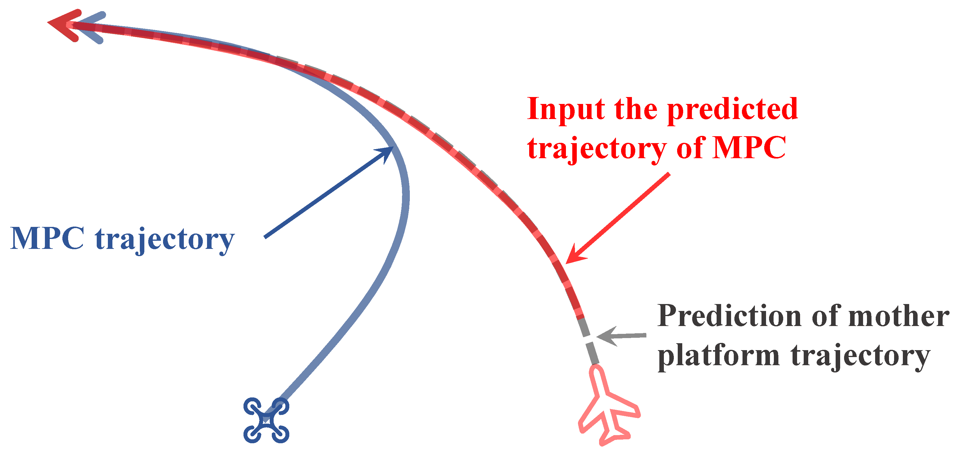
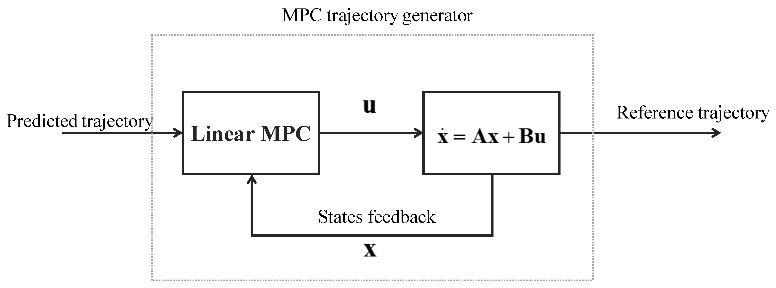
3.4. Linear MPC Trajectory Generator

Model predictive control (MPC), as an optimal control method in a finite time domain, is now widely used in the flight control of UAVs [1,24,25,26,27]. However, because a linear MPC cannot adapt to the nonlinear characteristics of the child UAV during high-speed flight, it is not directly involved in flight control in this paper but rather as a generator of reference states, as described in [15,16]. A linear MPC uses a linear model with n states and k inputs, defined as:

$$\begin{array}{cccc}\hfill & \hfill & \hfill {\mathbf{x}}_{\left[t+1\right]}& =\mathbf{A}{\mathbf{x}}_{\left[t\right]}+\mathbf{B}{\mathbf{u}}_{\left[t\right]},\hfill \end{array}$$

(15)

$$\begin{array}{cccc}\hfill & \hfill & \hfill {\mathbf{y}}_{\left[t\right]}& =\mathbf{C}{\mathbf{x}}_{\left[t\right]}+\mathbf{D}{\mathbf{u}}_{\left[t\right]},\hfill \end{array}$$

(16)

where $\mathbf{x}\in {\mathbb{R}}^n$ is the state vector and $\mathbf{u}\in {\mathbb{R}}^k$ is the input vector. Matrices $\mathbf{A}\in {\mathbb{R}}^{n\times n}$ and $\mathbf{B}\in {\mathbb{R}}^{n\times k}$ are the system matrix and input matrix, respectively. Because we want to observe the full states of the child UAV, we assume $\mathbf{C}=\mathbf{I}$ and $\mathbf{D}=\mathbf{0}$.

MPC computes the control input and plots the trajectory by minimizing the control error over the future prediction horizon. The control error is defined as $\mathbf{e}=\mathbf{x}-{\mathbf{x}}_{\mathrm{ref}}$ and the optimization problem is defined as:

$$\begin{array}{cc}\hfill \underset{{\mathbf{u}}_{\left[t\right]},{\mathbf{x}}_{\left[t\right]}}{min}\mathrm{V}\left(\mathbf{x},\mathbf{u}\right)=& \sum _{t=0}^T\left({\mathbf{e}}_{\left[t\right]}^{\top }\mathbf{Q}{\mathbf{e}}_{\left[t\right]}+{\mathbf{u}}_{\left[t\right]}^{\top }\mathbf{P}{\mathbf{u}}_{\left[t\right]}\right)+\hfill \end{array}\begin{array}{c}\hfill {\mathbf{e}}_{\left[T+1\right]}^{\top }{\mathbf{Q}}_{\mathrm{final}}{\mathbf{e}}_{\left[T+1\right]},\end{array}$$

(17)

$$\begin{array}{cc}\hfill \mathrm{s}.\mathrm{t}.{\mathbf{x}}_{\left[t+1\right]}=& \mathbf{A}{\mathbf{x}}_{\left[t\right]}+\mathbf{B}{\mathbf{u}}_{\left[t\right]},t=0,...,T,\hfill \end{array}$$

(18)

$$\begin{array}{cc}\hfill |{\mathbf{u}}_{\left[t\right]}|⩽& {\mathbf{u}}_{\max },t=0,...,T,\hfill \end{array}$$

(19)

$$\begin{array}{cc}\hfill \parallel {\mathbf{u}}_{\left[t+1\right]}& -{\mathbf{u}}_{\left[t\right]}\parallel ⩽\mathbf{S},t=0,...,T-1,\hfill \end{array}$$

(20)

$$\begin{array}{cc}\hfill {\mathbf{x}}_{\min }⩽& {\mathbf{x}}_{\left[t\right]}⩽{\mathbf{x}}_{\max },t=1,...,T+1,\hfill \end{array}$$

(21)

where the cost function in Equation (17) penalizes the control error, the terminal error, and the input action over a horizon T in length. Penalization matrices $\mathbf{Q}$, $\mathbf{P}$, and ${\mathbf{Q}}_{\mathrm{final}}$ are positive semidefinite. Equation (18) constraints follow the model in Equation (15). Equation (19) shows the constraints of the input action. Equation (20) shows the constraints of the magnitude of change in the input action. The maximum acceleration and velocity are limited by the constraints in Equation (21).

The MPC model in the linear MPC trajectory generator is the third-order linear model, the control inputs are the jerk, and the states are the position, velocity, and acceleration of the child UAV. The system matrix $\mathbf{A}$ and input matrix $\mathbf{B}$ are defined as:

$$\mathbf{A}=\left[\begin{array}{ccc}{\mathbf{A}}_s& \mathbf{0}& \mathbf{0}\\ \mathbf{0}& {\mathbf{A}}_s& \mathbf{0}\\ \mathbf{0}& \mathbf{0}& {\mathbf{A}}_s\end{array}\right], \mathbf{B}=\left[\begin{array}{ccc}{\mathbf{B}}_s& \mathbf{0}& \mathbf{0}\\ \mathbf{0}& {\mathbf{B}}_s& \mathbf{0}\\ \mathbf{0}& \mathbf{0}& {\mathbf{B}}_s\end{array}\right],$$

(22)

where sub-system matrices ${\mathbf{A}}_s$ and ${\mathbf{B}}_s$ are defined as:

$${\mathbf{A}}_s=\left[\begin{array}{ccc}1& \Delta t& \frac{\Delta t^2}{2}\\ 0& 1& \Delta t\\ 0& 0& 1\end{array}\right], \mathbf{B}=\left[\begin{array}{c}\frac{\Delta t^3}{6}\\ \frac{\Delta t^2}{2}\\ \Delta t\end{array}\right],$$

(23)

with $\Delta t$ being the MPC time step.

Figure 8 presents a diagram of the MPC trajectory generator shown as a single block in the pipeline in Figure 5. At a frequency of about 100 Hz, the linear MPC and kinematic model are used for closed-loop simulation, the predicted trajectory of the mother UAV is used as input, and the reference trajectory points are output to the trajectory tracking controller to guide the autonomous landing of the child UAV.

3.5. Vision-Based State Estimation of the Landing Platform

The final block is motion prediction of the mother UAV. As shown in Figure 3, the autonomous recovery process of the child UAV is divided into two stages: approaching and landing. Localization accuracy requirements are low in the approaching stage, and GPS and IMU are typically used for localization. Precision is essential during the landing stage. AprilTag visual localization is used to improve localization accuracy based on the size and cost of the child UAV. Since monocular visual localization can only provide relative position information between the camera and the target, we incorporated the global position of the child UAV, obtained by fusing GPS and IMU data during the landing stage, to determine the position of the recovery platform. Concurrently, a Kalman filter is used to estimate acceleration and jerk as well as obtain continuous state information. We use a nested tag for localization to avoid a decrease in the camera field of view of the child UAV as the altitude changes during the landing process, as shown in Figure 9.

The model for the Kalman filter is the three-order kinematic model in Equation (15). See previous research for more information on the use of Kalman filters for visual sensor localization [10,28]. However, in this paper, the Kalman filter is used to localize and predict the mother UAV. To obtain the full state information of the motion platform, the position and speed information of the onboard controller of the mother UAV are fused with the visual localization information, and the acceleration and jerk of the mother UAV are estimated at the same time. The algorithm flow of the Kalman filter is shown in Figure 10.

The Kalman filter outputs position, velocity, acceleration, and jerk of the mother UAV. The kinematic model Equations (24)–(26) can be used to predict the trajectory of the mother UAV over a time horizon. Finally, inputs of the MPC trajectory generator can be obtained.

$$\begin{array}{cccc}\hfill & \hfill & \hfill {\mathbf{p}}_{m\left[t+1\right]}& ={\mathbf{p}}_{m\left[t\right]}+{\mathbf{v}}_{m\left[t\right]}\Delta t+\frac{1}{2}{\mathbf{a}}_{m\left[t\right]}\Delta t^2+\frac{1}{6}{\mathbf{j}}_{m\left[t\right]}\Delta t^3,\hfill \end{array}$$

(24)

$$\begin{array}{cccc}\hfill & \hfill & \hfill {\mathbf{v}}_{m\left[t+1\right]}& ={\mathbf{v}}_{m\left[t\right]}+{\mathbf{a}}_{m\left[t\right]}\Delta t+\frac{1}{2}{\mathbf{j}}_{m\left[t\right]}\Delta t^2,\hfill \end{array}$$

(25)

$$\begin{array}{cccc}\hfill & \hfill & \hfill {\mathbf{a}}_{m\left[t+1\right]}& ={\mathbf{a}}_{m\left[t\right]}+{\mathbf{j}}_{m\left[t\right]}\Delta t.\hfill \end{array}$$

(26)

Figure 11 shows the prediction effects of Equations (24)–(26) on circular motion (10 m/s). Figure 11a,b show the position and velocity predictions, respectively. It can be seen that position and velocity of the third-order kinematics have nonlinear characteristics, demonstrating a good prediction effect on circular motion trajectories.

Figure 12a,b show the square root of position and velocity prediction errors ($error=\sqrt{e_x^2+e_y^2}$). It is clear that, as time passes, the prediction error increases rapidly. Fortunately, the position error is less than 0.01 m and the velocity error is less than 0.1 m/s within 40 time steps.

4. Simulation Experiments

In this section, we will perform software-in-the-loop simulation of the trajectory tracking controller, linear MPC trajectory generator, and control pipeline for the full-process autonomous landing mission, and verify the effect of the designed control law and control framework.

4.1. Implementation Details

The visual simulation environment for software-in-the-loop simulation is built on Gazebo and the onboard flight control is powered by Pixhawk 4. The linear MPC trajectory generator, trajectory tracking controller, and Kalman filter state estimation are built on ROS, and implemented using Python2.7 and C++. The solution of the linear MPC optimization problem is realized based on CVXGEN [29,30].

The MPC trajectory generator, trajectory tracking controller, Kalman filter, and trajectory prediction all run at 100 Hz in the simulation experiments.

Table 2. Gains and parameters of MPC generator and tracking controller.

MPC Trajectory Generator
$\mathbf{Q}={\mathbf{Q}}_{\mathrm{final}}$	$\mathrm{diag}(6000,3000,1800)$
$\mathbf{P}$	$\mathrm{diag}(5,5,5)$
$\mathbf{S}$	${\left[\begin{array}{ccc}0.1& 0.1& 0.1\end{array}\right]}^{\top }$
${\mathbf{u}}_{\max }$	${\left[\begin{array}{ccc}12.0& 12.0& 5.0\end{array}\right]}^{\top }$
${\mathbf{a}}_{\max }$	$\pm 12\mathrm{m}/{\mathrm{s}}^2$
${\mathbf{v}}_{\max }$	$\pm 20\mathrm{m}/\mathrm{s}$
T	40
$\Delta t$	$0.01$
Trajectory tracking controller
${\mathbf{K}}_{\mathrm{pos}}$	${\left[\begin{array}{ccc}6.78& 6.78& 13.5\end{array}\right]}^{\top }$
${\mathbf{K}}_{\mathrm{vel}}$	${\left[\begin{array}{ccc}3.0& 3.0& 6.0\end{array}\right]}^{\top }$
${\mathbf{K}}_{\mathrm{R}}$	$\pm 1.0$
$\mathbf{D}$	$\mathrm{diag}(0.45,0.35,0)$

shows the generator and controller parameters, while

Table 3. The child and mother UAVs configuration.

The child UAV
$\mathrm{Mass}\left[\mathrm{kg}\right]$	1
$\mathrm{Inertia}[\mathrm{kg}·{\mathrm{m}}^2]$	$\mathrm{diag}(0.0291,0.0291,0.0552)$
$\mathrm{Maximum}\mathrm{speed}[\mathrm{m}/\mathrm{s}]$	25
The mother UAV
$\mathrm{Mass}\left[\mathrm{kg}\right]$	5
$\mathrm{Span}\left[\mathrm{m}\right]$	$2.144$
$\mathrm{Inertia}[\mathrm{kg}·{\mathrm{m}}^2]$	$\mathrm{diag}(0.4777,0.3417,0.8110)$
$\mathrm{Circling}\mathrm{speed}[\mathrm{m}/\mathrm{s}]$	$11.5$

shows the main parameters of the child and mother UAVs.

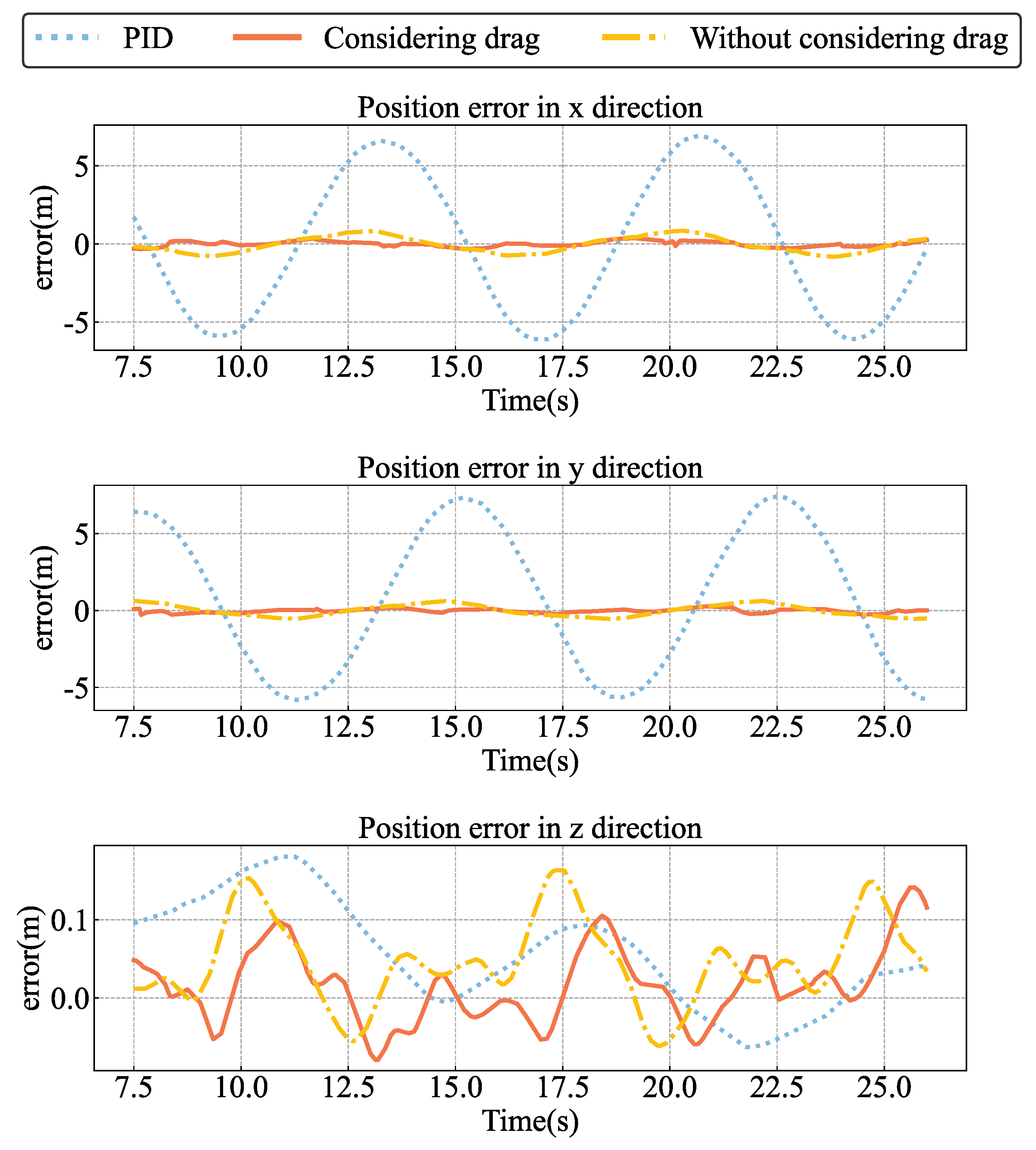
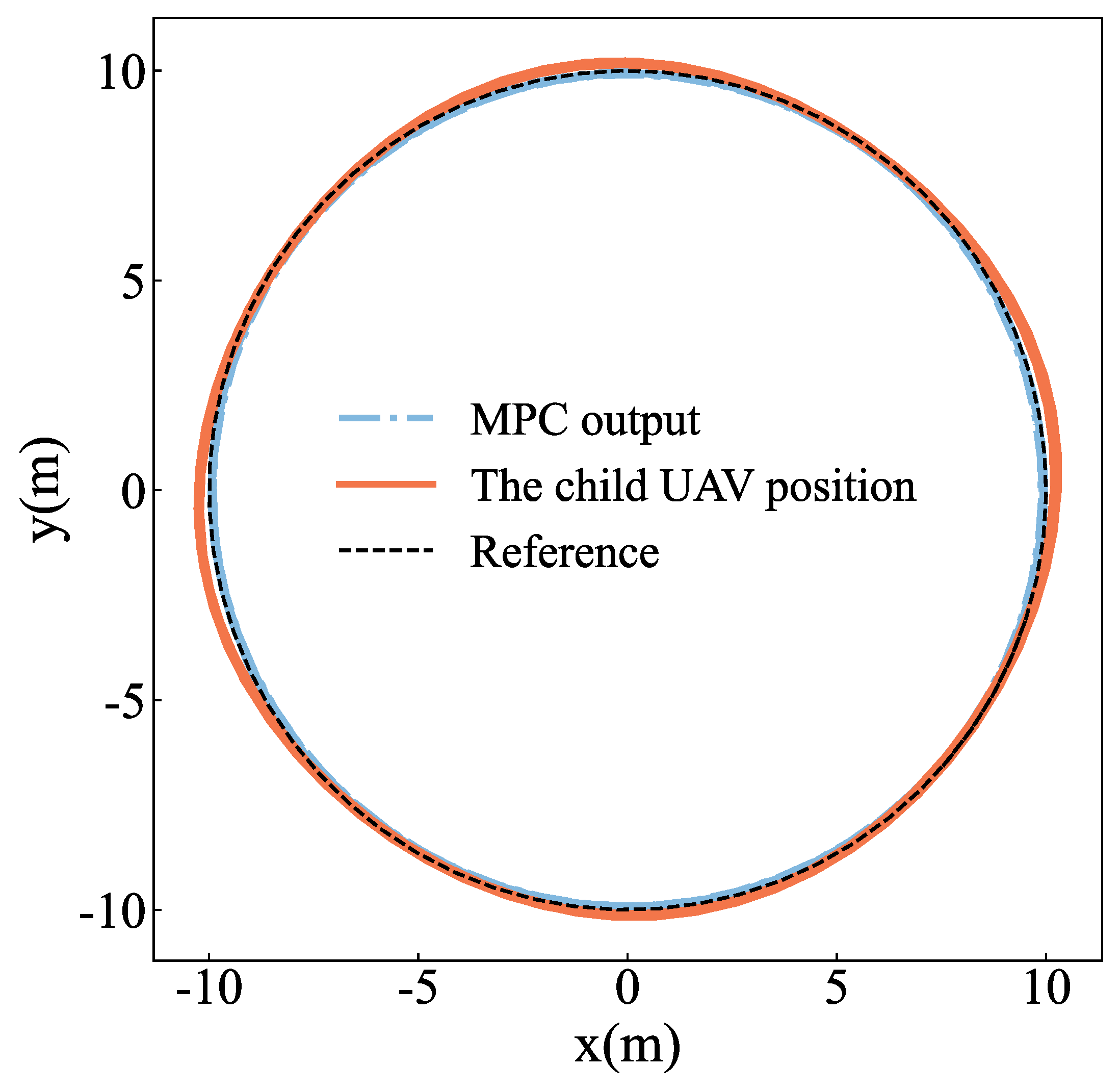
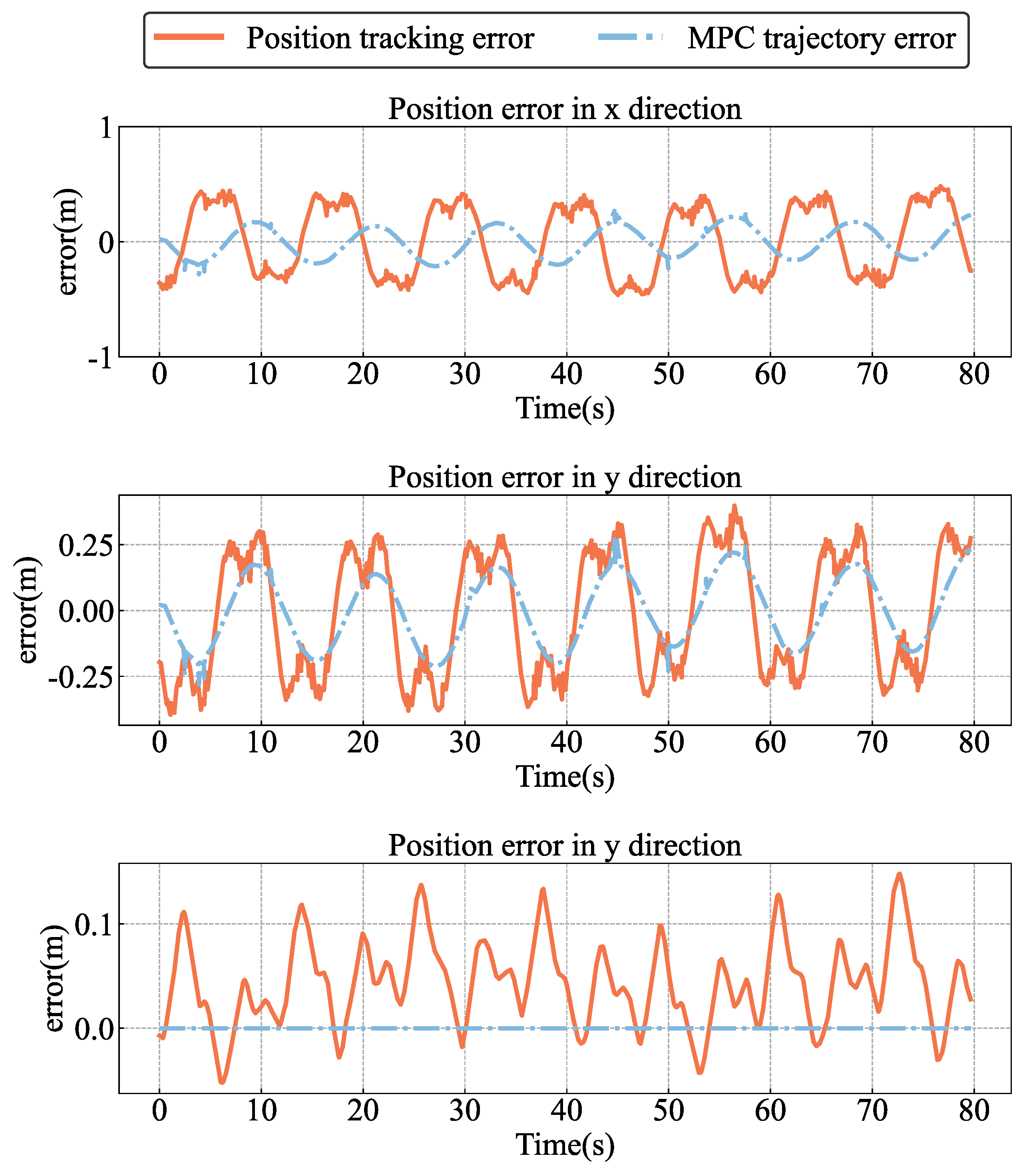
4.2. Trajectory Tracking Controller Evaluation

The basis for accurate tracking of the mother UAV by the child UAV is an accurate and fast-response trajectory tracking controller. In a software-in-the-loop simulation, we first assess the control effect of the trajectory tracking controller. In this simulation, the child UAV follows a circular path at a speed of 10 m/s. In the world frame, the reference trajectory is defined as:

$$\left[\begin{array}{c}x\\ y\\ z\end{array}\right]=\left[\begin{array}{c}10sin\left(t\right)\\ 10cos\left(t\right)\\ 0\end{array}\right].$$

(27)

We compared the PID controller with speed feedforward, the trajectory tracking controller without taking rotor drag into account, and the trajectory generator with rotor drag taken into account. It is worth noting that we used the cascade control structure of the PX4 open-source flight controller for the PID controller here [22]. According to our tests, the acceleration control of the PX4 is currently unavailable, so we just used velocity feedforward. The tracking results are shown in Figure 13.

The two nonlinear trajectory tracking controllers have significantly higher tracking accuracy than the PID controller with speed feedforward, as shown in Figure 13. Figure 14 shows the tracking errors of the three controllers. In order to further evaluate the tracking effect of the controller, the Mean Absolute Error (MAE) and the Maximum Error (${\mathrm{E}}_{\max }$) are introduced. The error performance of the three controllers is shown in

Table 4. Tracking errors of the three controllers relative to the reference trajectory.

Controller	ErrorType	x	y	z
$\mathrm{PID}$	$\mathrm{MAE}\left[\mathrm{m}\right]$	$4.070$	$4.207$	$0.060$
	${\mathrm{E}}_{\max }\left[\mathrm{m}\right]$	$7.024$	$7.510$	$0.181$
Considering drag	$\mathrm{MAE}\left[\mathrm{m}\right]$	0.176	0.113	0.042
	${\mathrm{E}}_{\max }\left[\mathrm{m}\right]$	0.391	0.303	0.142
Not considering drag	$\mathrm{MAE}\left[\mathrm{m}\right]$	$0.452$	$0.338$	$0.052$
	${\mathrm{E}}_{\max }\left[\mathrm{m}\right]$	$0.865$	$0.667$	$0.164$

.

Table 4 shows that the trajectory tracking controller with the smallest MAE and ${\mathrm{E}}_{\max }$ has the smallest rotor drag. It can be seen from Table 4 that the trajectory tracking controller considering the rotor drag has the smallest MAE and the ${\mathrm{E}}_{\max }$. When compared to the trajectory tracking controller that does not account for rotor resistance, the error is reduced by more than 50% after including rotor resistance compensation. This demonstrates that adding rotor drag compensation improved the controller’s tracking accuracy and demonstrated good control effect in the tracking of the high-speed circular trajectory.

4.3. MPC Trajectory Generator Evaluation

The linear MPC trajectory tracking controller is essential for producing a smooth recovery trajectory. Using the circular trajectory shown in Equation (24), we continue to evaluate the trajectory generation of the MPC trajectory generator. The MPC input is a reference trajectory for a time horizon and it outputs the desired trajectory points to the trajectory tracking controller, which keeps track of the desired trajectory points. Figure 15 shows the trajectory generated by MPC as well as the tracking effect of the child UAV.

As shown in Figure 16, the desired trajectory points output by the MPC and the tracking of the desired trajectory by the controller maintain a small error relative to the reference trajectory. Figure 16 shows the MPC trajectory tracking error and the position tracking error of the child UAV. It demonstrates that the proposed MPC trajectory generator can track the high-speed circular reference trajectory accurately.

Table 5. Position errors of the MPC generator and controller tracking relative to the reference trajectory.

	ErrorType	x	y	z
$\mathrm{MPC}$	$\mathrm{MAE}\left[\mathrm{m}\right]$	$0.148$	$0.143$	$0.0$
	${\mathrm{E}}_{\max }\left[\mathrm{m}\right]$	$0.299$	$0.332$	$0.0$
Trajectory tracking	$\mathrm{MAE}\left[\mathrm{m}\right]$	$0.248$	$0.212$	$0.049$
	${\mathrm{E}}_{\max }\left[\mathrm{m}\right]$	$0.484$	$0.398$	$0.148$

also displays the MAE and ${\mathrm{E}}_{\max }$ of MPC and trajectory tracking in comparison to the reference trajectory.

The tracking error of the reference trajectory increases significantly after adding the MPC trajectory generator when compared to the controller directly tracking the reference trajectory. Table 4 and Table 5 show that, when the MPC generator is added to the trajectory tracking controller, the average absolute error increases by about 40% and the maximum error increases by about 20% when compared to the trajectory tracking controller that considers the rotor resistance on average and directly tracks the reference trajectory. The main reason is that MPC is based on a linear kinematic model, and the circular trajectory still contains errors. At the same time, the real-time performance of the solution limits the optimization problem and the feasible solution may not be the optimal solution. Therefore, these factors contribute to the controller tracking error superposition.

However, the MPC trajectory generator must be added for the autonomous landing trajectory planning of the moving platform. Fortunately, the reference trajectory in the simulation and the circling flight trajectory of the fixed-wing UAV have higher centripetal acceleration and smaller flight radius, so the absolute error remains low under this condition. It is an acceptable range when compared to the position error constraint of 1 m (as shown in Table 1).

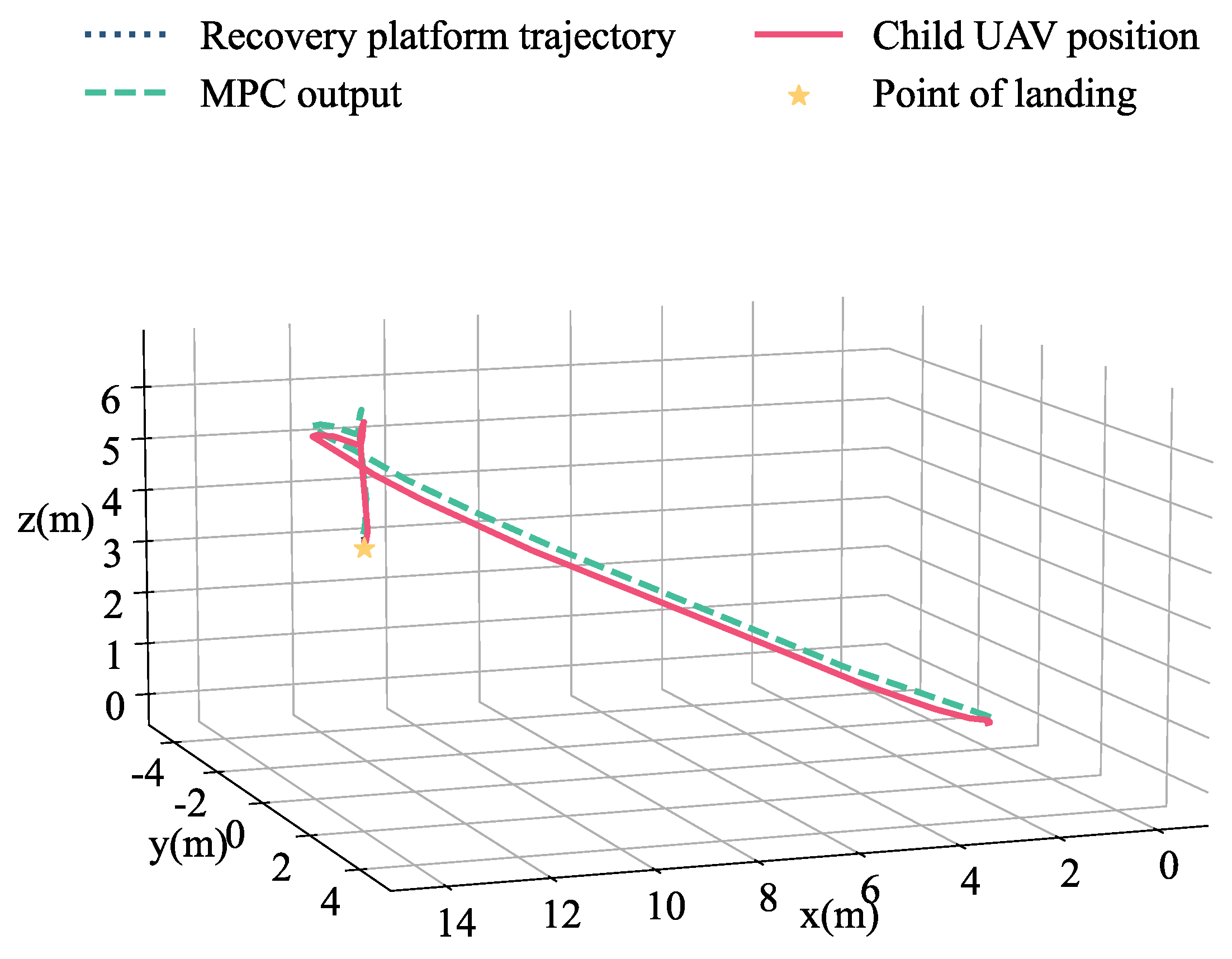
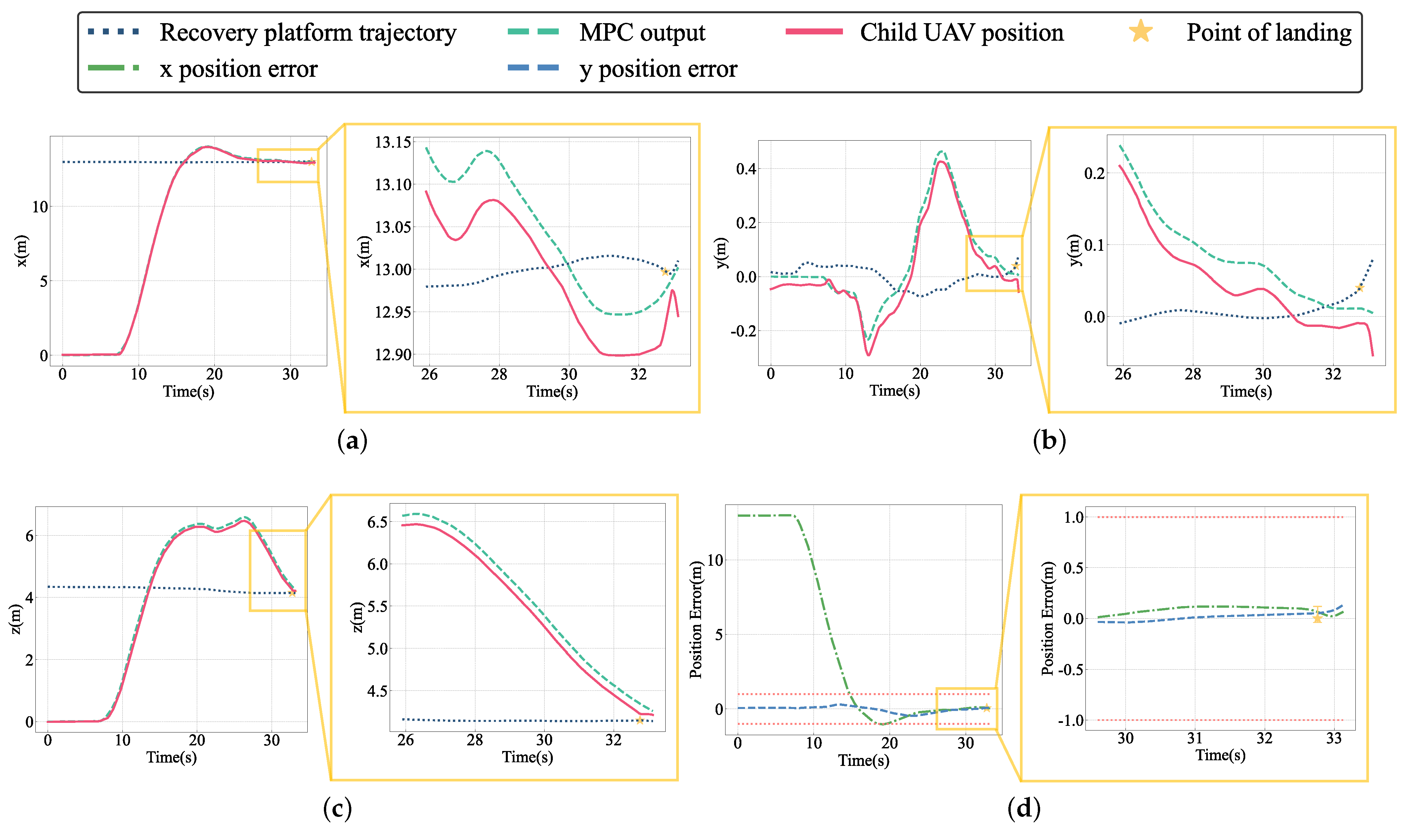
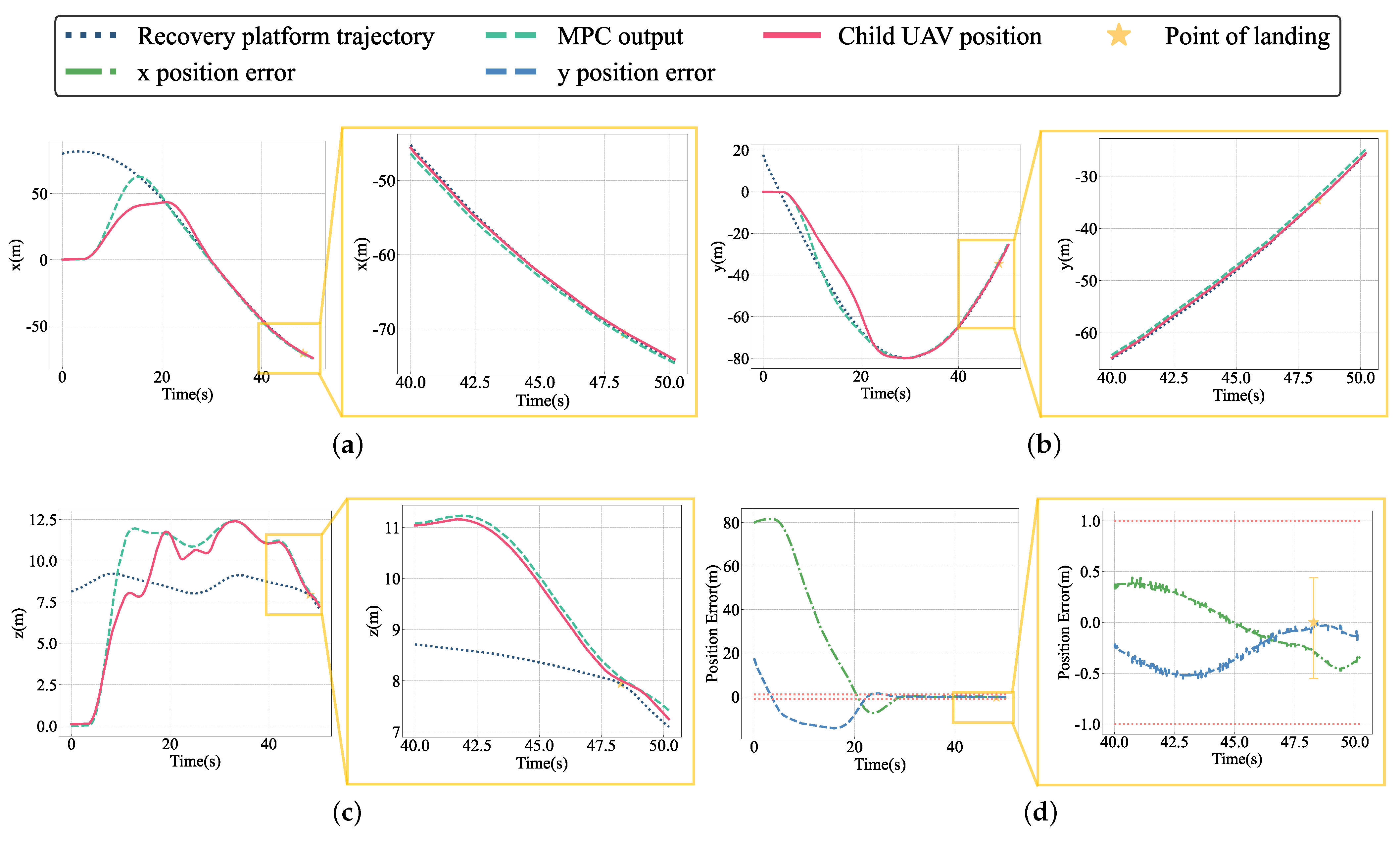
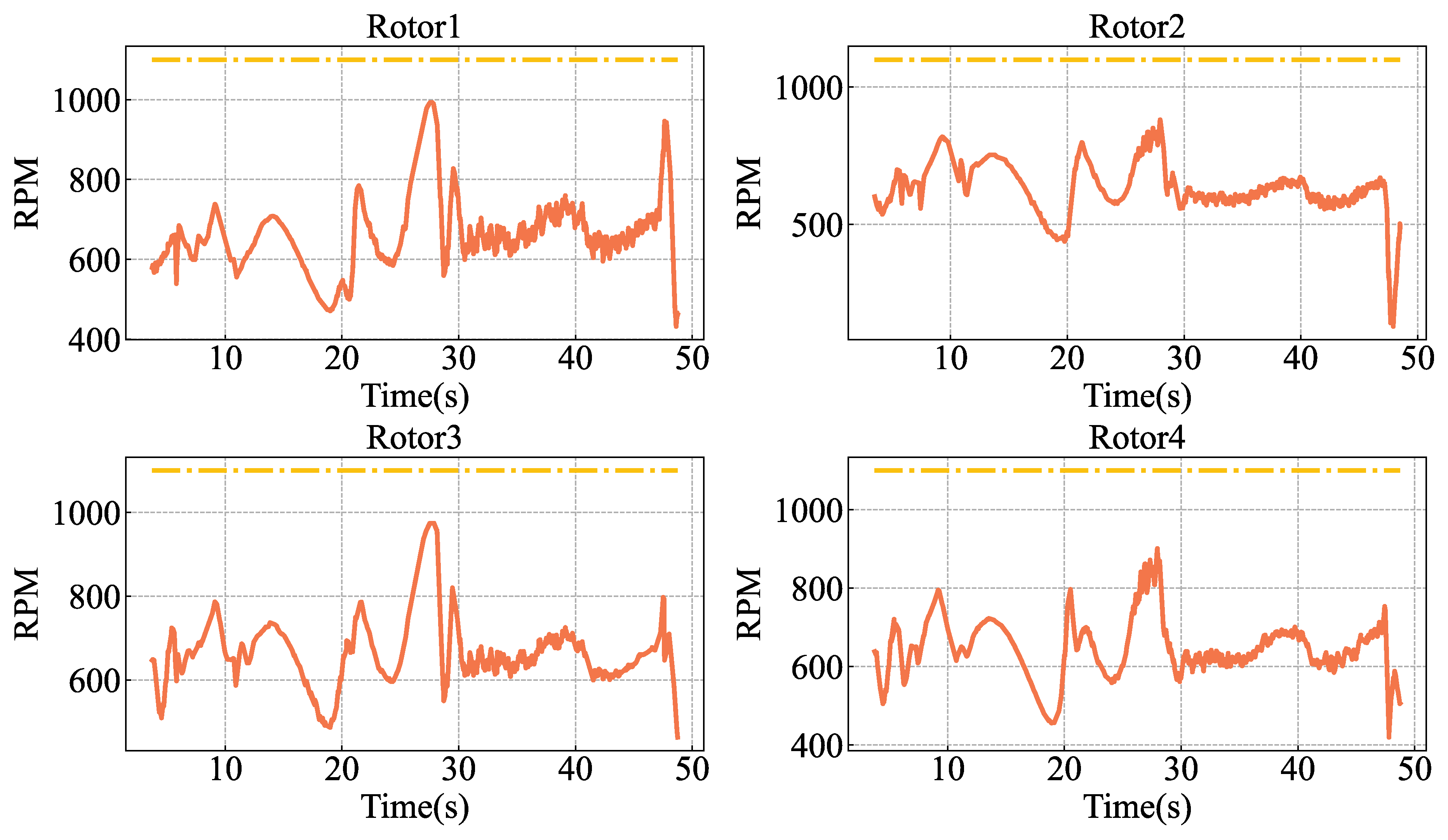
4.4. Autonomous Recovery Simulation

We evaluated the MPC trajectory generator and control algorithm in the preceding sections. We will simulate the entire mission process in this section to evaluate the autonomous recovery effect of the designed control architecture in both circling and hovering missions.

4.4.1. Recovery Mission in Hovering State

The take-off point of the child UAV serves as the origin of the world coordinate system in the simulation experiment. The mother UAV hovers around the world coordinates (13, 0, 4) during the hovering state recovery mission. When the recovery mission begins, the child UAV receives the mission start command, estimates the trajectory of the mother UAV using state estimation, and uses the trajectory of the mother UAV as the input of the MPC trajectory generator for a time horizon in the future. It should be noted that, in order to adapt to the subsequent recovery mission in high-speed circling state, and reduce the hysteresis error caused by feedback control and inaccurate modeling of the child UAV during high-speed movement, the MPC trajectory generator uses the mother UAV as input instead of 0–0.4 s. Because the mother UAV hovers practically motionlessly, the advanced trajectory input will not produce visible position errors. The MPC plans the desired trajectory based on the predicted trajectory and tracks it using the trajectory tracking controller. The desired trajectory keeps the UAV at a safe distance of 2.5 m from the recovery platform. Following that, the child UAV follows the desired trajectory and hovers above the recovery platform, maintains a safe height, and keeps track of the recovery platform in the horizontal direction. After receiving the landing recovery command, the child UAV began landing on the recovery platform of the mother UAV and landed in about 36 s. The 3D trajectory of the recovery mission in the hovering state is shown in Figure 17.

When the mother UAV is hovering, the 3D recovery trajectory shows the movement state of the child UAV and the desired trajectory in space. We can obtain the curve of the position in the three directions with time by decomposing the position in the three directions of x, y, and z, as shown in Figure 18.

As shown in Figure 18a–c, the MPC trajectory generator generates a smooth recovery trajectory, guiding the child UAV to a hovering landing on the mother UAV. After receiving the recovery command, the child UAV immediately flies to the mother UAV from the origin, maintaining a close track on the planned trajectory. After the landing, the obvious deviation of the position is because the recovery platform defined in the simulation only has collision properties, so, after the mother and child UAV contact, the child UAV slides on the platform and the model interferes. This has no bearing on the recovery process.

As shown in Figure 18d, the horizontal tracking error approaches 0 m at around 25 s. After 25 s, the horizontal position error is substantially less than 1 m, till the last child UAV complete landing. This demonstrates that the controller has a decent position tracking effect and can keep a small position tracking error while hovering. Although the movement state between the child UAV and the recovery platform in the hovering state is relatively constant, the relative speed of the two is still analyzed to determine whether the recovery end is reasonably static. The relative velocities of the child UAV and the recovery platform in both the x and y directions are shown in Figure 19.

As shown in Figure 19a, the child UAV and the recovery platform are seen at the start of the recovery stage (5–15 s). At this point, the child UAV is closing in on the mother UAV. The relative speed of the child UAV in the x direction increases significantly at the end of recovery because the child UAV is in partial contact with the recovery platform at this time, and the interference of the model and collision appear in the simulation, resulting in an increase in the speed in the x direction, but still within 0.25 m. Figure 19b shows the change in speed in the y direction. Because the recovery platform has no position error with the child UAV in the y direction, the relative speed is kept within a narrow range. The relative speed error is depicted in Figure 19c. The relative speed between the recovery platform and the child UAV is definitely less than 0.5 m/s near the landing point at the recovery end.

Figure 20 illustrates the evolution of the four motor speeds of the child UAV during the recovery process. As the UAV maintains a stable flight condition throughout the mission, the motor speeds consistently hover around 500 RPM, with no control signal saturation. The simulation results show that, despite being designed for the high dynamic recovery mission of fixed-wing circling, the autonomous recovery control system still has a good effect when faced with a relatively static recovery platform in the hovering state and can adapt to different state recovery missions.

4.4.2. Recovery Mission in Circling State

For the recovery mission in the circling state, the mother UAV has a more complex motion state. The mother UAV has a radius of approximately 78 m, a flight speed of approximately 11.5 m/s, and a flying height of approximately 8 m as it rounds the origin of the world coordinate system. The process of the recovery mission is basically the same as recovery in the hovering state. It should be noted here that the MPC trajectory generator uses the predicted trajectory of the mother UAV in the future 0.15–0.55 s as input rather than 0–0.4 s. The MPC plans the desired trajectory based on the predicted trajectory and tracks it using the trajectory tracking controller. The desired trajectory keeps the UAV at a safe distance of 2.5 m from the recovery platform. Following that, the child UAV follows the desired trajectory and ascends above the recovery platform, maintains a safe height, and keeps track of the recovery platform in the horizontal direction. After receiving the landing recovery command, the child UAV began landing on the recovery platform of the mother UAV and landed in about 48 s. The 3D trajectory of the recovery mission is shown in Figure 21.

When the mother UAV is circling, the 3D recovery trajectory shows the entire recovery process of the child UAV as well as the desired trajectory output by the MPC. We can obtain the curve of the position in the three directions with time by decomposing the position in the three directions of x, y, and z, as shown in Figure 22.

As shown in Figure 22a–c, the MPC trajectory generator generates a smooth recovery trajectory, guiding the child UAV to a hovering landing on the mother UAV. The tracking effect of the child UAV is poor between 5 and 20 s because the trajectory planned by the MPC based on the kinematic model is very aggressive at this time. When approaching the recovery platform, the speed and acceleration tend to flatten, and the tracking effect is significantly improved, allowing the recovery end error to be met.

As shown in Figure 22d, the horizontal position error quickly converges to 0 m and stabilizes in the interval of (−1 m, 1 m). The influence of sensor noise on positioning information can be clearly seen in the local error curve of about 40–50 s. After 40 s, the position error in the x and y directions is always stable in the (−1 m, 1 m) interval, meeting the landing recovery error requirement of 1 m. The proposed control architecture can meet the current recovery control accuracy requirements in position control, as demonstrated by the position and position error curves. However, for our mission, not only is a small relative position error required but the relative velocity error at the recovery end must also be kept to a minimum. The relative velocities of the child UAV and the recovery platform in both the x and y directions are shown in Figure 23.

As shown in Figure 23a,b, the tracking effect is also poor in the early stages of tracking due to the aggressive trajectory. With the convergence of position error, the child UAV has a relatively accurate tracking effect on the horizontal speed of the recovery platform. The small fluctuation in speed at the end of the landing is caused by contact between the child UAV and the recovery platform at this time. The velocity error is shown in Figure 23c throughout the recovery mission. After about 30 s, the speed error has stabilized within 1 m/s and, at the end of the landing, the speed error is within 0.5 m/s.

Figure 24 illustrates the fluctuation in the rotor speeds of the child UAV during the recovery process while the mother UAV circles overhead. The aggressive flight trajectory leads to significant variations in rotor speeds (the highest speed of Motor1 is about 1000 RPM). However, due to the kinematic constraints imposed by the trajectory generation, the rotor speeds remain below saturation. It is crucial to acknowledge the potentially devastating impact of control signal saturation on system stability, making it imperative to avoid saturation in practical applications. Experimental findings in reference [31] highlight the system’s instability following motor saturation. Moreover, as indicated in reference [32], when the controller reaches saturation, the original stability proof may no longer hold, necessitating exploration of stability in saturated states. Therefore, the introduction of dynamically feasible constraints in trajectory generation is essential. These constraints play a pivotal role in maintaining system stability, mitigating the adverse effects of signal saturation, and ensuring the robustness of the control system.

Based on the above, it can be demonstrated that the autonomous recovery control framework designed in this paper has an accurate position tracking effect and a good speed tracking effect on the recovery platform, and that it is capable of effectively realizing the autonomous landing of the child UAV. To further validate the robustness of the control system, we ran 20 simulation experiments on autonomous recovery missions; the child UAV was successfully recovered 16 times and the other 4 times a second recovery was necessary due to the loss of visual positioning tags during the landing process.

5. Discussion

In comparison to previous work [33], this study adds a control framework that may be applied to the autonomous recovery mission of a child UAV on an aerial recovery platform while hovering or moving at least 11 m/s. Our developed trajectory tracking controller with rotor drag performs well in high-speed flight and can achieve accurate tracking of high-speed motion trajectories in the control framework. Meanwhile, we employ the motion trajectory prediction of the recovery platform as input to the MPC trajectory generator, thus avoiding trajectory generation time estimation. The tracking accuracy of the recovery platform can be successfully increased by modifying the input time horizon of the anticipated trajectory. We used software-in-the-loop simulation to test the effectiveness of the control framework multiple times. The simulation results show that the framework can generate smooth real-time landing trajectories and keep accurate track of the desired trajectories.

However, the existing model is incapable of simulating turbulence interference around the recovery platform, communication delays, and other real-world challenges. In the future, we will perform numerical simulations of turbulence interference near the aerial recovery platform, followed by real-world flight experiments to validate the effectiveness of the proposed control system.

References

1. Petrlik, M.; Baca, T.; Hert, D.; Vrba, M.; Krajnik, T.; Saska, M. A Robust UAV System for Operations in a Constrained Environment. IEEE Robot. Autom. Lett. 2020, 5, 2169–2176. [Google Scholar] [CrossRef]
2. Zhang, H.T.; Hu, B.B.; Xu, Z.; Cai, Z.; Liu, B.; Wang, X.; Geng, T.; Zhong, S.; Zhao, J. Visual Navigation and Landing Control of an Unmanned Aerial Vehicle on a Moving Autonomous Surface Vehicle via Adaptive Learning. IEEE Trans. Neural Netw. Learn. Syst. 2021, 32, 5345–5355. [Google Scholar] [CrossRef] [PubMed]
3. Narvaez, E.; Ravankar, A.A.; Ravankar, A.; Kobayashi, Y.; Emaru, T. Vision Based Autonomous Docking of VTOL UAV Using a Mobile Robot Manipulator. In Proceedings of the 2017 IEEE/SICE International Symposium on System Integration (SII), IEEE, Taipei, Taiwan, 11–14 December 2017; pp. 157–163. [Google Scholar]
4. Ghommam, J.; Saad, M. Autonomous Landing of a Quadrotor on a Moving Platform. IEEE Trans. Aerosp. Electron. Syst. 2017, 53, 1504–1519. [Google Scholar] [CrossRef]
5. Guo, K.; Tang, P.; Wang, H.; Lin, D.; Cui, X. Autonomous Landing of a Quadrotor on a Moving Platform via Model Predictive Control. Aerospace 2022, 9, 34. [Google Scholar] [CrossRef]
6. Olson, E. AprilTag: A Robust and Flexible Visual Fiducial System. In Proceedings of the 2011 IEEE International Conference on Robotics and Automation, IEEE, Shanghai, China, 9–13 May 2011; pp. 3400–3407. [Google Scholar]
7. Wang, J.; Olson, E. AprilTag 2: Efficient and Robust Fiducial Detection. In Proceedings of the 2016 IEEE/RSJ International Conference on Intelligent Robots and Systems (IROS), IEEE, Daejeon, Republic of Korea, 9–14 October 2016; pp. 4193–4198. [Google Scholar]
8. Krogius, M.; Haggenmiller, A.; Olson, E. Flexible Layouts for Fiducial Tags. In Proceedings of the 2019 IEEE/RSJ International Conference on Intelligent Robots and Systems (IROS), IEEE, Macau, China, 3–8 November 2019; pp. 1898–1903. [Google Scholar]
9. Xu, G.; Qi, X.; Zeng, Q.; Tian, Y.; Guo, R.; Wang, B. Use of Land’s Cooperative Object to Estimate UAV’s Pose for Autonomous Landing. Chin. J. Aeronaut. 2013, 26, 1498–1505. [Google Scholar] [CrossRef]
10. Zhenglong, G.; Qiang, F.; Quan, Q. Pose Estimation for Multicopters Based on Monocular Vision and AprilTag. In Proceedings of the 2018 37th Chinese Control Conference (CCC), IEEE, Wuhan, China, 25–27 July 2018; pp. 4717–4722. [Google Scholar]
11. Brommer, C.; Malyuta, D.; Hentzen, D.; Brockers, R. Long-Duration Autonomy for Small Rotorcraft UAS Including Recharging. In Proceedings of the 2018 IEEE/RSJ International Conference on Intelligent Robots and Systems (IROS), IEEE, Madrid, Spain, 1–5 October 2018; pp. 7252–7258. [Google Scholar]
12. Mohammadi, A.; Feng, Y.; Zhang, C.; Rawashdeh, S.; Baek, S. Vision-Based Autonomous Landing Using an MPC-controlled Micro UAV on a Moving Platform. In Proceedings of the 2020 International Conference on Unmanned Aircraft Systems (ICUAS), IEEE, Athens, Greece, 1–4 September 2020; pp. 771–780. [Google Scholar]
13. Ji, J.; Yang, T.; Xu, C.; Gao, F. Real-Time Trajectory Planning for Aerial Perching. In Proceedings of the 2022 IEEE/RSJ International Conference on Intelligent Robots and Systems (IROS), Kyoto, Japan, 23–27 October 2022; pp. 10516–10522. [Google Scholar]
14. Vlantis, P.; Marantos, P.; Bechlioulis, C.P.; Kyriakopoulos, K.J. Quadrotor Landing on an Inclined Platform of a Moving Ground Vehicle. In Proceedings of the 2015 IEEE International Conference on Robotics and Automation (ICRA), IEEE, Seattle, WA, USA, 26–30 May 2015; pp. 2202–2207. [Google Scholar]
15. Baca, T.; Hert, D.; Loianno, G.; Saska, M.; Kumar, V. Model Predictive Trajectory Tracking and Collision Avoidance for Reliable Outdoor Deployment of Unmanned Aerial Vehicles. In Proceedings of the 2018 IEEE/RSJ International Conference on Intelligent Robots and Systems (IROS), IEEE, Madrid, Spain, 1–5 October 2018; pp. 6753–6760. [Google Scholar]
16. Baca, T.; Stepan, P.; Spurny, V.; Hert, D.; Penicka, R.; Saska, M.; Thomas, J.; Loianno, G.; Kumar, V. Autonomous Landing on a Moving Vehicle with an Unmanned Aerial Vehicle. J. Field Robot. 2019, 36, 874–891. [Google Scholar] [CrossRef]
17. Paris, A.; Lopez, B.T.; How, J.P. Dynamic Landing of an Autonomous Quadrotor on a Moving Platform in Turbulent Wind Conditions. In Proceedings of the 2020 IEEE International Conference on Robotics and Automation (ICRA), Paris, France, 31 May–31 August 2020; pp. 9577–9583. [Google Scholar]
18. Rodriguez-Ramos, A.; Sampedro, C.; Bavle, H.; Milosevic, Z.; Garcia-Vaquero, A.; Campoy, P. Towards Fully Autonomous Landing on Moving Platforms for Rotary Unmanned Aerial Vehicles. In Proceedings of the 2017 International Conference on Unmanned Aircraft Systems (ICUAS), IEEE, Miami, FL, USA, 13–16 June 2017; pp. 170–178. [Google Scholar]
19. Falanga, D.; Zanchettin, A.; Simovic, A.; Delmerico, J.; Scaramuzza, D. Vision-Based Autonomous Quadrotor Landing on a Moving Platform. In Proceedings of the 2017 IEEE International Symposium on Safety, Security and Rescue Robotics (SSRR), IEEE, Shanghai, China, 11–13 October 2017; pp. 200–207. [Google Scholar]
20. Faessler, M.; Franchi, A.; Scaramuzza, D. Differential Flatness of Quadrotor Dynamics Subject to Rotor Drag for Accurate Tracking of High-Speed Trajectories. IEEE Robot. Autom. Lett. 2018, 3, 620–626. [Google Scholar] [CrossRef]
21. Lee, T.; Leok, M.; McClamroch, N.H. Geometric Tracking Control of a Quadrotor UAV on SE(3). In Proceedings of the 49th IEEE Conference on Decision and Control (CDC), IEEE, Atlanta, GA, USA, 15–17 December 2010; pp. 5420–5425. [Google Scholar]
22. Meier, L.; Honegger, D.; Pollefeys, M. PX4: A Node-Based Multithreaded Open Source Robotics Framework for Deeply Embedded Platforms. In Proceedings of the 2015 IEEE International Conference on Robotics and Automation (ICRA), IEEE, Seattle, WA, USA, 26–30 May 2015; pp. 6235–6240. [Google Scholar]
23. Sun Yang, C.M.; Junqiang, B. Trajectory planning and control for micro-quadrotor perching on vertical surface. Acta Aeronaut. Astronaut. Sin. 2022, 43, 325756. [Google Scholar]
24. Koubaa, A. Robot Operating System (ROS): The Complete Reference (Volume 2). In Studies in Computational Intelligence; Springer International Publishing: Cham, Switzerland, 2017; Volume 707. [Google Scholar]
25. Baca, T.; Loianno, G.; Saska, M. Embedded Model Predictive Control of Unmanned Micro Aerial Vehicles. In Proceedings of the 2016 21st International Conference on Methods and Models in Automation and Robotics (MMAR), IEEE, Miedzyzdroje, Poland, 29 August–1 September 2016; pp. 992–997. [Google Scholar]
26. Ardakani, M.M.G.; Olofsson, B.; Robertsson, A.; Johansson, R. Real-Time Trajectory Generation Using Model Predictive Control. In Proceedings of the 2015 IEEE International Conference on Automation Science and Engineering (CASE), IEEE, Gothenburg, Sweden, 24–28 August 2015; pp. 942–948. [Google Scholar]
27. Cagienard, R.; Grieder, P.; Kerrigan, E.; Morari, M. Move Blocking Strategies in Receding Horizon Control. J. Process. Control 2007, 17, 563–570. [Google Scholar] [CrossRef]
28. Janabi-Sharifi, F.; Marey, M. A Kalman-Filter-Based Method for Pose Estimation in Visual Servoing. IEEE Trans. Robot. 2010, 26, 9. [Google Scholar] [CrossRef]
29. Mattingley, J.; Boyd, S. CVXGEN: A code generator for embedded convex optimization. Optim. Eng. 2012, 13, 1–27. [Google Scholar] [CrossRef]
30. Mattingley, J.; Yang, W.; Boyd, S. Code generation for receding horizon control. In Proceedings of the 2010 IEEE International Symposium on Computer-Aided Control System Design (CACSD), Yokohama, Japan, 8–10 September 2010. [Google Scholar]
31. Horla, D.; Hamandi, M.; Giernacki, W.; Franchi, A. Optimal Tuning of the Lateral-Dynamics Parameters for Aerial Vehicles with Bounded Lateral Force. IEEE Robot. Autom. Lett. 2021, 6, 3949–3955. [Google Scholar] [CrossRef]
32. Shen, Z.; Ma, Y.; Tsuchiya, T. Stability Analysis of a Feedback-linearization-based Controller with Saturation: A Tilt Vehicle with the Penguin-inspired Gait Plan. arXiv 2021, arXiv:2111.14456. [Google Scholar]
33. Du, D.; Chang, M.; Bai, J.; Xia, L. Autonomous Recovery System of Aerial Child-Mother Unmanned Systems Based on Visual Positioning. In Proceedings of the 2022 International Conference on Autonomous Unmanned Systems (ICAUS 2022), Online Event, 22–26 May 2022; Fu, W., Gu, M., Niu, Y., Eds.; Springer Nature Singapore: Singapore, 2023; pp. 1787–1797. [Google Scholar]
Figure 1. Visual simulation environment. Based on Robot Operating System (ROS), Pixhawk 4 and Gazebo.
Drones 07 00648 g001
Figure 2. The MPC trajectory generator. The solid blue line represents the reference trajectory output from the trajectory generator. The gray dotted line represents the mother platform’s motion trajectory over a period of time. The solid red line represents the desired trajectory as input to the MPC trajectory generator.
Drones 07 00648 g002
Figure 3. Autonomous landing process division. GPS is used to obtain the position information of the mother platform during the approaching stage, and obtain the position information of the mother platform through vision and GPS during the landing stage.
Drones 07 00648 g003
Figure 5. Diagram of the control pipeline, including the Kalman filter, the proposed MPC trajectory generator, and trajectory tracking controller.
Drones 07 00648 g005
Figure 6. The child UAV from take-off to landing is controlled by the state machine. The state machine enables the child UAV to complete the second landing when visual localization is lost.
Drones 07 00648 g006
Figure 7. Diagram of the trajectory tracking controller.
Drones 07 00648 g007
Figure 8. Diagram of the MPC trajectory generator.
Drones 07 00648 g008
Figure 9. The nested tag of AprilTag.
Drones 07 00648 g009
Figure 10. The algorithm flow of the Kalman filter.
Drones 07 00648 g010
Figure 11. Prediction effect of three–order linear model on circular motion trajectory. (a) Position prediction on the horizontal plane. (b) Velocity prediction on the horizontal plane.
Drones 07 00648 g011
Figure 12. Prediction error for a third order linear equation. (a) Square root of position prediction error in the horizontal plane. (b) Square root of velocity prediction error in the horizontal plane.
Drones 07 00648 g012
Figure 13. The tracking position for the PID controller (dashed blue), the tracking controller with the rotor drag (solid orange), and the tracking controller without considering the rotor drag (dashed yellow) compared to the reference position (dashed black).
Drones 07 00648 g013
Figure 14. Tracking errors of PID controller, and tracking controller with drag and without drag to track circular reference trajectory.
Drones 07 00648 g014
Figure 15. The tracking position for the tracking controller with the rotor drag (solid orange) and the desired trajectory points of MPC (dashed blue) compared to the reference position (dashed black).
Drones 07 00648 g015
Figure 16. Position tracking error and MPC trajectory generator error.
Drones 07 00648 g016
Figure 17. The 3D trajectory of the recovery mission in the hovering state, including the trajectory of the recovery platform (dashed navy blue), the desired trajectory output by the MPC trajectory generator (dashed blue green), the position of the child drone (solid red), and the landing point (yellow star).
Drones 07 00648 g017
Figure 18. The motion trajectory in the three directions of the world frame and the error in the horizontal direction in the hovering state: (a) x-axis direction position curve; (b) y-axis direction position curve; (c) z-axis direction position curve; (d) position error in the horizontal direction.
Drones 07 00648 g018
Figure 19. The relative speed and relative speed error of horizontal plane of the world coordinate system in the hovering state: (a) x-axis direction velocity curve; (b) y-axis direction velocity curve; (c) z-axis direction velocity curve.
Drones 07 00648 g019
Figure 20. Motor RPM (solid orange) for each motor of the child UAV during the recovery mission, with the mother UAV in a hovering state. Each motor has a maximum rotor speed of 1100 RPM (dashed yellow).
Drones 07 00648 g020
Figure 21. The 3D trajectory of the recovery mission in the circling state, including the trajectory of the recovery platform (dashed navy blue), the desired trajectory output by the MPC trajectory generator (dashed blue green), the position of the child drone (solid red), and the landing point (yellow star).
Drones 07 00648 g021
Figure 22. The motion trajectory in the three directions of the world frame and the error in the horizontal direction in the circling state: (a) x-axis direction position curve; (b) y-axis direction position curve; (c) z-axis direction position curve; (d) position error in the horizontal direction.
Drones 07 00648 g022
Figure 23. The velocity in the horizontal plane of the world frame and the velocity error in the horizontal direction: (a) x-axis direction velocity curve; (b) y-axis direction velocity curve; (c) z-axis direction velocity curve.
Drones 07 00648 g023
Figure 24. Motor RPM (solid orange) for each motor of the child UAV during the recovery mission, with the mother UAV in a circling state. Each motor has a maximum rotor speed of 1100 RPM (dashed yellow).
Drones 07 00648 g024