Robust Collision-Free Guidance and Control for Underactuated Multirotor Aerial Vehicles

Abstract

This paper is concerned with the robust collision-free guidance and control of underactuated multirotor aerial vehicles in the presence of moving obstacles capable of accelerating, linear velocity and rotor thrust constraints, and matched model uncertainties and disturbances. We address this problem by using a hierarchical flight control architecture composed of a supervisory outer-loop guidance module and an inner-loop stabilizing control one. The inner loop is designed using a typical hierarchical control scheme that nests the attitude control loop inside the position one. The effectiveness of this scheme relies on proper time-scale separation (TSS) between the closed-loop (faster) rotational and (slower) translational dynamics, which is not straightforward to enforce in practice. However, by combining an integral sliding mode attitude control law, which guarantees instantaneous tracking of the attitude commands, with a smooth and robust position control one, we enforce, by construction, the satisfaction of the TSS, thus avoiding the loss of robustness and use of a dull trial-and-error tweak of gains. On the other hand, the outer-loop guidance is built upon the continuous-control-obstacles method, which is incremented to respect the velocity and actuator constraints and avoid multiple moving obstacles that can accelerate. The overall method is evaluated using a numerical Monte Carlo simulation and is shown to be effective in providing satisfactory tracking performance, collision-free guidance, and the satisfaction of linear velocity and actuator constraints.

1. Introduction

Multirotor aerial vehicles (MAVs) have been extensively researched in recent decades and are expected to be widely used for a variety of new, challenging applications, such as delivery [1] and air taxis [2]. These applications demand a high level of safety and are usually carried out in disturbed environments where the MAV may fly among obstacles such as buildings, other manned or unmanned aircraft, and birds. To enable dependable operation, the MAV flight control system must provide outstanding performance, robustness, and collision avoidance. Aiming at contributing to this topic, this paper focuses on underactuated MAVs equipped with fixed rotors (which includes the conventional and widespread quadrotor). We start by adopting a typical hierarchical guidance and control architecture [3], such as the one shown in Figure 1. This architecture is composed of an outer-loop guidance system whose goal is to conduct the vehicle to the desired state while avoiding collisions and respecting operational and physical constraints. It also contains an inner control loop providing stability and robustness.

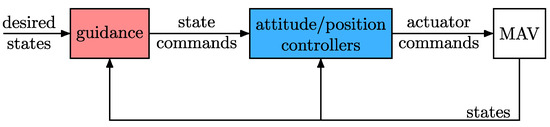
Figure 1. A typical hierarchical guidance and control architecture for MAVs.

To address the robustness requirement of MAV flight control systems against model uncertainties and disturbances, the sliding mode control [4,5] (SMC) strategy has been widely adopted to design the position and attitude control laws [6,7,8,9,10,11]. This technique provides a high-frequency switching control signal to drive and keep a system output on a sliding manifold, where the system ideally becomes insensitive to bounded model uncertainties and disturbances of the matched type. In particular, there are also SMC design techniques based on sliding manifolds suitably constructed to eliminate the reaching phase, i.e., to enable a sliding motion (with the insensitivity property) from the very beginning [12,13,14,15,16]. These design techniques can be found in the literature under two main alternative designations: the integral sliding mode control (ISMC) [14] and sometimes the global sliding mode control (GSMC) [13,16].

To deal with the underactuated dynamics of the considered class of MAVs, most of the literature relies on the assumption of time-scale separation (TSS) between the (slower) position and (faster) attitude closed-loop dynamics [6,7,8,9,17,18,19,20,21], which allows us to nest the attitude control loop inside the position one. As a consequence, the position and attitude control laws can be designed separately, but their gains have to be suitably tuned to achieve a sufficient TSS. In particular, the use of SMC in underactuated control systems is still a challenge [22]. In fact, under this nested control architecture, by using a high-frequency switching signal in the outer-loop position control law, it is not possible to properly guarantee the required TSS since such a signal is too fast to be considered slow in the design of the inner-loop attitude control. Nevertheless, there is no restriction on the use of such a policy in the attitude control. In this context, Besnard et al. [6] designed flight controllers using a continuous SMC driven by a sliding mode disturbance observer (SMDO). A procedure to tune the controllers’ gains in order to respect the TSS between the control loops was presented. Muñoz Palacios et al. [7] adopted a modified super-twisting SMC driven by a high-order sliding mode observer. Silva and Santos [8] and Labbadi and Cherkaoui [9] designed nonsingular fast terminal sliding mode flight control laws, but, to avoid the TSS violation, the position control loop was smoothed using sigmoid functions at the cost of robustness. It is worth noting that all the above-cited methods demand a trial-and-error procedure for the tuning of the flight control laws to respect the TSS assumption and avoid eventual instability.

The guidance of MAVs among obstacles has been addressed in the literature using different methods, such as nonlinear model predictive control (NMPC) [23,24], sampling-based search [25], and velocity obstacles (VO) [26,27,28]. In particular, Kamel et al. [23] and Pereira et al. [24] employed an NMPC to guide an MAV through static obstacles, addressing the collision avoidance problem by using a penalty in the cost function. Furthermore, Bouzid et al. [25] guided an MAV among static obstacles by combining an optimal rapidly exploring random tree (RRT) method with a genetic algorithm to compute the shortest path to a given target. On the other hand, Bareiss and Van Den Berg [27] proposed the linear–quadratic regulator obstacles (LQR obstacles) to address collision avoidance for mobile robots described by linear dynamics, rather than by single integrators as in the original VO [26]. The method was evaluated using quadcopters whose nonlinear dynamics were supposed to be known and linearized around the hover state. Other methods, such as the acceleration velocity obstacles (AVO) [29] and continuous control obstacles (CCO) [30], were also developed as generalizations of the VO to deal with more complicated known linear dynamics. Among the references [23,24,25,27], only [27] addresses the guidance problem for MAVs in the presence of moving obstacles. However, they use a simplified dynamic model and, like the VO-based methods [26,29,30], predict the obstacles’ future positions assuming that they keep a constant velocity, which is generally not satisfied in practice, but is addressed using a quick replanning loop with no guarantee that collision can be avoided when the obstacles accelerate.

This paper tries to fill the aforementioned gaps in the current state of the art by addressing the guidance and control for underactuated MAVs subject to matched model uncertainties and disturbances, as well as velocity and rotor thrust constraints, in the presence of obstacles that can accelerate. To tackle this problem, we start by adopting the hierarchical architecture shown in Figure 1 [3]. To design the position and attitude control laws, we propose a new hierarchical SMC scheme that, differently from [6,7,8,9,10], enforces the TSS without losing robustness and using a dull trial-and-error tweak of gains. Under this scheme, the attitude control law is designed using an ISMC strategy, in such a way as to guarantee exact tracking capability in the attitude control loop during the entire time, under the condition that the attitude command is sufficiently smooth. Then, this smoothness requirement is fulfilled by designing the position control law using a proportional–derivative (PD) approach combined with an SMDO to endow the position control loop with robustness. By doing so, the TSS is instantaneously enforced since the inner loop is made infinitely fast. On the other hand, we propose a nonlinear and robust guidance strategy based on the CCO method [30]. The guidance considers the use of smooth reference filters and, rather than relying on overly simplified nominal dynamics, it is able to deal with the uncertain nonlinear system dynamics. These system dynamics, as seen by the guidance algorithm, encompass the reference filters and the translational and rotational control loops, including the uncertainties and disturbances. Then, using the fact that the TSS is enforced by the control strategy, we tighten the admissible sets according to the bounds of the MAV tracking errors as well as the bounds of the disturbance force and torque. By doing so, different from that of Bareiss and Van Den Berg [27], the proposed strategy is able to guarantee collision avoidance and the satisfaction of velocity and rotor thrust constraints for underactuated MAVs with uncertain dynamics. Furthermore, to reliably address the problem of collision avoidance in the presence of obstacles that can accelerate, we adopt our previous method [28] that uses a high-order sliding mode differentiator (SMD) [31,32] to robustly estimate the obstacles’ maximum accelerations. Then, using these estimates, the obstacles’ future positions are not predicted using first-order models, as generally done in the VO-based methods [26,27,29,30], but considering the obstacles’ maximum accelerations. To summarize, the main contributions of this paper are the proposal of

• a hierarchical SMC scheme to design the position and attitude control laws for underactuated MAVs that, by construction, enforces the TSS assumption and
• robust guidance, based on the CCO and designed using a constraint-tightening approach, for underactuated MAVs with uncertain dynamics in the presence of velocity and rotor thrust constraints and multiple moving obstacles capable of accelerating.

The remaining text is structured as follows. Section 1.1 presents the notation. Section 2 defines the problem. Section 3 and Section 4 present, respectively, the control and guidance methods. Section 5 evaluates the proposed method using numerical simulations. Lastly, Section 6 concludes the paper.

1.1. Notation

The sets of real numbers, positive real numbers, and non-negative real numbers are denoted by $\mathbb{R}$, ${\mathbb{R}}_{>0}$, and ${\mathbb{R}}_{\ge 0}$, respectively. In the same manner, the sets of integer numbers, positive integer numbers, and non-negative integer numbers are denoted by $\mathbb{Z}$, ${\mathbb{Z}}_{>0}$, and ${\mathbb{Z}}_{\ge 0}$, respectively. Uppercase and lowercase boldface letters are used, respectively, to denote matrices and algebraic vectors, while geometric (Euclidean) vectors are denoted as in $\overrightarrow{a}$. The symbols ${\mathbf{I}}_n$ and ${\mathbf{0}}_{n\times m}$ denote, respectively, the $n\times n$ identity matrix and the $n\times m$ zero matrix. Moreover, the vectors of ones and zeros of dimension n are denoted, respectively, by ${\mathbf{1}}_n$ and ${\mathbf{0}}_n$. A Cartesian coordinate system (CCS) is represented as ${\mathcal{S}}_b\triangleq \{B;{\overrightarrow{x}}_b,{\overrightarrow{y}}_b,{\overrightarrow{z}}_b\}$, with B denoting its origin and ${\overrightarrow{x}}_b$, ${\overrightarrow{y}}_b$, and ${\overrightarrow{z}}_b$ representing the unit geometric vectors along its orthogonal axes. The algebraic vectors corresponding to the projection of an arbitrary physical vector $\overrightarrow{a}\in {\mathbb{R}}^3$ onto ${\mathcal{S}}_b$ and ${\mathcal{S}}_r$ are denoted, respectively, by ${\mathbf{a}}_b\in {\mathbb{R}}^3$ and ${\mathbf{a}}_r\in {\mathbb{R}}^3$. The relation between ${\mathbf{a}}_r$ and ${\mathbf{a}}_b$ is ${\mathbf{a}}_b={\mathbf{D}}^{b/r}{\mathbf{a}}_r$, where ${\mathbf{D}}^{b/r}\in \mathrm{SO}\left(3\right)$ is the attitude matrix of ${\mathcal{S}}_b$ relative to ${\mathcal{S}}_r$ and $\mathrm{SO}\left(3\right)\triangleq \{\mathbf{D}\in {\mathbb{R}}^{3\times 3}|{\mathbf{D}}^{\mathrm{T}}\mathbf{D}={\mathbf{I}}_3\}$ denotes the special orthogonal group. The inverse of ${\mathbf{D}}^{b/r}$ is equal to its transpose, being denoted by ${\mathbf{D}}^{r/b}$. Let ${\overrightarrow{a}}^{b/r}$ represent an arbitrary quantity of ${\mathcal{S}}_b$ relative to ${\mathcal{S}}_r$, e.g., throughout this paper, ${\overrightarrow{r}}^{b/r}$ will denote the position of ${\mathcal{S}}_b$ with respect to ${\mathcal{S}}_r$. Consider two arbitrary algebraic vectors $\mathbf{x}=(x_1,\dots ,x_n)$ and $\mathbf{y}=(y_1,\dots ,y_n)$. The vector inequality $\mathbf{x}<\mathbf{y}$ means that $x_i<y_i$, $\forall i\in \{1,\dots ,n\}$. The kth-order time derivative of $\mathbf{x}$ is denoted by ${\mathbf{x}}^{\left(k\right)}$. Furthermore, we define the vector signum function as $\mathrm{sign}\left(\mathbf{x}\right)\triangleq (\mathrm{sign}\left(x_1\right),\dots ,\mathrm{sign}\left(x_n\right))$, where

$$\mathrm{sign}\left(x_i\right)\triangleq \left\{\begin{array}{cc}1\hfill & x_i>0,\hfill \\ 0\hfill & x_i=0,\hfill \\ -1\hfill & x_i<0,\hfill \end{array}\right.$$

with $i\in \{1,\dots ,n\}$. The Euclidean norm and component-wise absolute value of $\mathbf{x}$ are denoted, respectively, by $\parallel \mathbf{x}\parallel \triangleq \sqrt{x_1^2+\dots +x_n^2}$ and $\left|\mathbf{x}\right|\triangleq \left(\right|x_1|,\dots ,|x_n\left|\right)$. On the other hand, the component-wise absolute value of a generic matrix $\mathbf{A}\in {\mathbb{R}}^{m\times n}$ is $\left|\mathbf{A}\right|\triangleq \left(|A_{i,j}|\right)\in {\mathbb{R}}^{m\times n}$, where $A_{i,j}$ is the element of the ith row and jth column of $\mathbf{A}$. The standard basis vectors of ${\mathbb{R}}^3$ are denoted by ${\mathbf{e}}_1\triangleq \left(1,0,0\right)$, ${\mathbf{e}}_2\triangleq \left(0,1,0\right)$, and ${\mathbf{e}}_3\triangleq \left(0,0,1\right)$. A closed sphere of radius $\rho \in {\mathbb{R}}_{>0}$ centered at $\mathbf{p}\in {\mathbb{R}}^3$, the Minkowski sum of two sets, and the set subtraction are denoted, respectively, by

$$\begin{array}{cc}\hfill \mathcal{B}\left(\mathbf{p},\rho \right)& =\left\{\mathbf{x}\in {\mathbb{R}}^3|∥\mathbf{x}-\mathbf{p}∥\le \rho \right\},\hfill \\ \hfill \mathcal{X}\oplus \mathcal{Y}& =\left\{\mathbf{x}+\mathbf{y}|\mathbf{x}\in \mathcal{X},\mathbf{y}\in \mathcal{Y}\right\},\hfill \\ \hfill \mathcal{X}\setminus \mathcal{Y}& =\left\{\mathbf{x}|\mathbf{x}\in \mathcal{X},\mathbf{x}\notin \mathcal{Y}\right\}.\hfill \end{array}$$

Finally, consider the ${\mathcal{S}}_r$ representations ${\mathbf{a}}_r$ and ${\mathbf{b}}_r\triangleq \left(b_1,b_2,b_3\right)$ of $\overrightarrow{a}$ and $\overrightarrow{b}$, respectively. The vector product $\overrightarrow{c}=\overrightarrow{b}\times \overrightarrow{a}$ is represented in ${\mathcal{S}}_r$ by ${\mathbf{c}}_r=\left[{\mathbf{b}}_r\times \right]{\mathbf{a}}_r$, where $\left[{\mathbf{b}}_r\times \right]$ is the following skew-symmetric matrix:

$$\left[{\mathbf{b}}_r\times \right]\triangleq \left[\begin{array}{ccc}0& -b_3& b_2\\ b_3& 0& -b_1\\ -b_2& b_1& 0\end{array}\right].$$

2. Problem Definition

This section defines the main problem of the paper. First, the MAV translational and rotational dynamics are derived in Section 2.1. Second, the control and guidance problems are stated in Section 2.2.

2.1. MAV Dynamic Modeling

Consider an inertial reference CCS ${\mathcal{S}}_r\triangleq \left\{R;{\overrightarrow{x}}_r,{\overrightarrow{y}}_r,{\overrightarrow{z}}_r\right\}$ fixed on the ground at a known point R, with ${\overrightarrow{z}}_r$ oriented upwards, parallel to the local vertical. Moreover, consider a body-fixed CCS ${\mathcal{S}}_b\triangleq \left\{B;{\overrightarrow{x}}_b,{\overrightarrow{y}}_b,{\overrightarrow{z}}_b\right\}$ located at a point B fixed to the MAV center of mass, as shown in Figure 2, along with an illustration of a general underactuated MAV equipped with $n_r\ge 4$ fixed rotors parallel to ${\overrightarrow{z}}_b$.

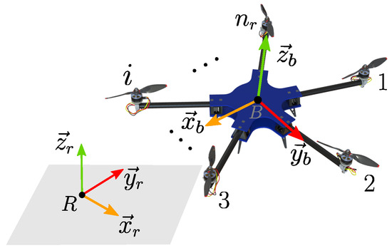
Figure 2. The adopted CCSs and a general underactuated MAV equipped with $n_r$ fixed rotors parallel to ${\overrightarrow{z}}_b$.

The attitude kinematics of ${\mathcal{S}}_b$ with respect to ${\mathcal{S}}_r$ can be described in SO(3) by [33]

$${\dot{\mathbf{D}}}^{b/r}=-\left[{\mathit{\omega }}_b^{b/r}\times \right]{\mathbf{D}}^{b/r},$$

(1)

where ${\mathbf{D}}^{b/r}\in \mathrm{SO}\left(3\right)$ and ${\mathit{\omega }}_b^{b/r}\in {\mathbb{R}}^3$ are, respectively, the attitude matrix and the angular velocity of the MAV.

Using the Euler equation [34], the MAV rotational dynamics can be described by

$${\dot{\mathbf{h}}}_b+{\mathit{\omega }}_b^{b/r}\times {\mathbf{h}}_b={\mathit{\tau }}_b^c+{\mathit{\tau }}_b^d,$$

(2)

where ${\mathbf{h}}_b\in {\mathbb{R}}^3$ is the angular momentum of the MAV relative to point B, ${\mathit{\tau }}_b^c\in {\mathbb{R}}^3$ is the control torque, and ${\mathit{\tau }}_b^d\in {\mathbb{R}}^3$ is the disturbance torque, which can include state-dependent terms related to parametric and model uncertainties [11]; both torques are with respect to B. Assuming a rigid airframe and negligible rotor inertias, the angular momentum ${\mathbf{h}}_b$ can be written as

$${\mathbf{h}}_b={\mathbf{J}}_b{\mathit{\omega }}_b^{b/r},$$

(3)

where ${\mathbf{J}}_b\in {\mathbb{R}}^{3\times 3}$ is the MAV inertia tensor.

By substituting (3) into (2), the rotational dynamics can be finally described by

$${\dot{\mathit{\omega }}}_b^{b/r}={\mathbf{J}}_b^{-1}\left[{\mathbf{J}}_b{\mathit{\omega }}_b^{b/r}\times \right]{\mathit{\omega }}_b^{b/r}+{\mathbf{J}}_b^{-1}\left({\mathit{\tau }}_b^c+{\mathit{\tau }}_b^d\right).$$

(4)

The translational kinematics of ${\mathcal{S}}_b$ relative to ${\mathcal{S}}_r$, on the other hand, are represented by

$${\dot{\mathbf{r}}}_r^{b/r}={\mathbf{v}}_r^{b/r},$$

(5)

where ${\mathbf{r}}_r^{b/r}\in {\mathbb{R}}^3$ and ${\mathbf{v}}_r^{b/r}\in {\mathbb{R}}^3$ are, respectively, the position and linear velocity of the MAV.

Using Newton’s second law, the translational dynamics of the MAV can be described in ${\mathcal{S}}_r$ by

$${\dot{\mathbf{v}}}_r^{b/r}=-g{\mathbf{e}}_3+m^{-1}\left({\mathbf{f}}_r^c+{\mathbf{f}}_r^d\right),$$

(6)

where $g\in {\mathbb{R}}_{>0}$ is the gravity acceleration magnitude, $m\in {\mathbb{R}}_{>0}$ is the MAV mass, ${\mathbf{f}}_r^c\in {\mathbb{R}}^3$ is the control force, and ${\mathbf{f}}_r^d\in {\mathbb{R}}^3$ is the disturbance force, which can include state-dependent terms related to parametric and model uncertainties.

The set of Equations (1) and (4)–(6) can be used to represent the six-degrees-of-freedom (DOF) dynamics of any fixed-rotor rigid MAV with negligible rotor inertia, regardless of its rotor configuration. For the considered class of underactuated MAVs, the control force is given by

$${\mathbf{f}}_r^c=f{\mathbf{n}}_r,$$

(7)

where ${\mathbf{n}}_r\triangleq {\mathbf{D}}^{r/b}{\mathbf{e}}_3$ is the ${\mathcal{S}}_r$ representation of ${\overrightarrow{z}}_b$ and $f\triangleq \parallel {\mathbf{f}}_r^c\parallel$ is the resultant thrust magnitude.

Denote by $f_i\in \mathbb{R}$ the thrust of the ith rotor and define the vector ${\mathbf{f}}^r\triangleq (f_1,f_2,\dots ,f_{n_r})$. The control allocation equation relating f and ${\mathit{\tau }}_b^c$ with ${\mathbf{f}}^r$ is [35]

$$\left[\begin{array}{c}f\\ {\mathit{\tau }}_b^c\end{array}\right]=\mathbf{\Gamma }{\mathbf{f}}^r,$$

(8)

where $\mathbf{\Gamma }\in {\mathbb{R}}^{4\times n_r}$ is the control allocation matrix, which depends on the rotors’ coefficients and arrangement. For the considered class of underactuated MAVs, $\mathbf{\Gamma }$ is always of full-row rank, i.e., $\mathrm{rank}\left(\mathbf{\Gamma }\right)=4$, thus allowing the rotors to produce, within certain limits, a three-dimensional torque and a resultant thrust in the ${\overrightarrow{z}}_b$ direction.

The resulting system (1), (4)–(8) is said to be underactuated since it has only four control inputs, ${\mathit{\tau }}_b^c$ and f, to control a six-DOF motion. Furthermore, from (6) and (7), it can be seen that the translational dynamics depend on the MAV attitude. For this reason, we can say that the rotational and translational dynamics are cascaded.

2.2. Problem Statement

Consider that the MAV is subject to velocity and rotor thrust constraints and flies among moving obstacles. These circumstances give rise to the following constraints:

$$\begin{array}{cc}\hfill {\mathbf{r}}_r^{b/r}& \in \mathcal{P}\left(t\right),\hfill \end{array}$$

(9)

$$\begin{array}{cc}\hfill {\mathbf{v}}_r^{b/r}& \in \mathcal{V},\hfill \end{array}$$

(10)

$$\begin{array}{cc}\hfill {\mathbf{f}}^r& \in \mathcal{F},\hfill \end{array}$$

(11)

where $\mathcal{P}\left(t\right)\subseteq {\mathbb{R}}^3$ denotes the collision-free space, which changes as the obstacles move and is generally non-convex; $\mathcal{V}\subseteq {\mathbb{R}}^3$ is an admissible convex set; and $\mathcal{F}$ is assumed to be

$$\mathcal{F}\triangleq \left\{{\mathbf{f}}^r\in {\mathbb{R}}^{n_r}|f_i\in \left[f_i^{-},f_i^{+}\right],\forall i\in \{1,\dots ,n_r\}\right\},$$

being $f_i^{-}\in {\mathbb{R}}_{>0}$ and $f_i^{+}\in {\mathbb{R}}_{>0}$, respectively, the given lower and upper bounds for the ith rotor thrust.

Let us define the heading angle $\psi \in [-\pi ,\pi )$ as the third rotation in the 1-2-3 Euler angle representation of the MAV attitude.

Denoting the MAV’s desired (constant) position and desired (constant) heading, respectively, by ${\check{\mathbf{r}}}_r^{b/r}\in {\mathbb{R}}^3$ and $\check{\psi }\in [-\pi ,\pi )$, we now define the main problem of the paper.

Problem 1. 

Guide the underactuated MAV described by (1), (4)–(8) to precisely reach the desired position ${\check{\mathit{r}}}_r^{b/r}$ and the desired heading $\check{\psi }$, while satisfying constraints (9)–(11).

Problem 1 is a nonlinear guidance and control problem of an underactuated MAV subject to disturbances and constraints, operating in a dynamic environment with multiple moving obstacles that can accelerate. To tackle this problem, we adopt the guidance and control architecture shown in Figure 1. The adopted strategy is to design the control module to provide robustness with respect to disturbances and uncertainties, and the guidance module to satisfy the position, velocity, and rotors’ thrust constraints while conducting the vehicle to reach the desired position and heading. The control and guidance methods are, respectively, detailed in Section 3 and Section 4. It is worth mentioning that the objective of Problem 1 can be immediately generalized for a sequence of desired positions and headings [3].

3. Control Design

This section presents the design of the position and attitude control laws to address Problem 1. Specifically, Section 3.1 introduces the adopted hierarchical flight control architecture. Section 3.2 formulates the attitude control law. Section 3.3 formulates the position control law. Lastly, Section 3.4 presents the control allocation.

Before proceeding to the next subsection, let us denoted the command of a given variable by using an overbar symbol, e.g., ${\overline{\mathbf{r}}}_r^{b/r}$ and $\overline{\psi }$ denote the position and heading commands, respectively.

3.1. Hierarchical Flight Control Architecture

Most of the literature on underactuated MAVs [6,7,8,9,17,18,19,20,21] has designed the position and attitude controllers relying on a TSS between the (slower) position and (faster) attitude closed-loop dynamics, which allows us to nest the attitude control loop inside the position one, as shown in the block diagram of Figure 3. In this architecture, the position controller receives ${\overline{\mathbf{r}}}_r^{b/r}$ as the command input, ${\mathbf{r}}_r^{b/r}$ and ${\mathbf{v}}_r^{b/r}$ as feedback, and produces ${\overline{\mathbf{f}}}_r^c$ as the output. The attitude command generator (ACG) converts ${\overline{\mathbf{n}}}_r$ and $\overline{\psi }$ into the three-dimensional attitude command ${\overline{\mathbf{D}}}^{b/r}$. The attitude controller receives ${\overline{\mathbf{D}}}^{b/r}$ as the command input, ${\mathbf{D}}^{b/r}$ and ${\mathit{\omega }}_b^{b/r}$ as feedback, and produces ${\overline{\mathit{\tau }}}_b^c$ as output. Lastly, the control allocation converts $\overline{f}$ and ${\overline{\mathit{\tau }}}_b^c$ into individual thrust commands ${\overline{\mathbf{f}}}^r\triangleq \left({\overline{f}}_1,\dots ,{\overline{f}}_{n_r}\right)$.

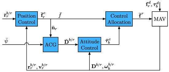
Figure 3. Hierarchical control architecture for underactuated MAVs equipped with fixed rotors. ACG stands for attitude command generator.

Consider the following assumption regarding the rotors.

Assumption 1. 

The rotor dynamics are instantaneous and their static parameters are exactly known.

Assumption 1 is common in practice since the rotor dynamics are much faster than the attitude and position ones, thus allowing us to suppose, in the design of the controllers, that the thrust commands are instantaneously achieved, i.e., ${\mathbf{f}}^r\equiv {\overline{\mathbf{f}}}^r,\forall t\ge 0$. Consequently, from (8), one can say that $f\equiv \overline{f}$ and ${\mathit{\tau }}_b^c\equiv {\overline{\mathit{\tau }}}_b^c$.

By assuming that the rotational dynamics are faster than the translational ones, the TSS allows consideration in the design of the position controller that ${\mathbf{n}}_r={\overline{\mathbf{n}}}_r$. Then, by also considering Assumption 1, Equation (7) becomes

$${\mathbf{f}}_r^c=\overline{f}{\overline{\mathbf{n}}}_r\triangleq {\overline{\mathbf{f}}}_r^c,$$

(12)

where ${\overline{\mathbf{n}}}_r\equiv {\overline{\mathbf{D}}}^{r/b}{\mathbf{e}}_3$, which in theory removes the underactuation of the system since the dependency of ${\mathbf{f}}_r^c$ on the actual attitude is removed. Then, the attitude and position control laws can be separately designed by considering the resulting fully actuated system described by Equations (1), (4)–(6), and (12). The critical point is that, when using this strategy, the controllers’ gains have to be carefully tuned in order to respect the TSS assumption, whereas, in practice, this tuning is a cumbersome trial-and-error process, thus requiring improved safety procedures to deal with the eventual instability that may occur in the case of insufficient TSS [36].

To avoid this drawback, we propose a hierarchical sliding mode control scheme for underactuated MAVs that enforces the attitude-position TSS. To this end, we design a multi-input attitude control law using an ISMC strategy, in such a way as to guarantee exact tracking capability in the attitude control loop during all the time. Such exact tracking makes ${\mathbf{n}}_r={\overline{\mathbf{n}}}_r$ without the need for tuning to reach the TSS. Therefore, the position control law can be designed using the fully actuated system described by (5), (6), and (12).

3.2. Integral Sliding Mode Attitude Control Law

Consider the objective of tracking a time-varying attitude command ${\overline{\mathbf{D}}}^{b/r}$ that satisfies the following assumption.

Assumption 2. 

The time-varying attitude command ${\overline{\mathit{D}}}^{b/r}$ is such that, at the initial time, ${\overline{\mathit{D}}}^{b/r}\left(0\right)={\mathit{D}}^{b/r}\left(0\right)$ and ${\overline{\mathit{\omega }}}_b^{b/r}\left(0\right)={\mathit{\omega }}_b^{b/r}\left(0\right)$. Moreover, it is $(h-1)$th-order differentiable with respect to time, where $h\ge 2$, such that its first-time derivative ${\dot{\overline{\mathit{D}}}}^{b/r}$ is Lipschitz-continuous.

Assumption 2 is not restrictive; it only requires the knowledge of the MAV’s initial attitude and angular velocity and the use of a suitably smooth attitude command. These conditions can be fulfilled by properly designing the heading command $\overline{\psi }$ and the position control law (see Figure 3).

The attitude and angular velocity control errors can be defined, respectively, as [33]

$$\begin{array}{cc}\hfill \tilde{\mathbf{D}}& \triangleq {\mathbf{D}}^{b/\overline{b}}\equiv {\mathbf{D}}^{b/r}{\left({\overline{\mathbf{D}}}^{b/r}\right)}^{\mathrm{T}}\in \mathrm{SO}\left(3\right),\hfill \end{array}$$

(13)

$$\begin{array}{cc}\hfill \tilde{\mathit{\omega }}& \triangleq {\mathit{\omega }}_b^{b/\overline{b}}\equiv {\mathit{\omega }}_b^{b/r}-\tilde{\mathbf{D}}{\overline{\mathit{\omega }}}_b^{b/r}\in {\mathbb{R}}^3,\hfill \end{array}$$

(14)

where ${\overline{\mathbf{D}}}^{b/r}\triangleq {\mathbf{D}}^{\overline{b}/r}$, ${\overline{\mathit{\omega }}}_b^{b/r}\triangleq {\mathit{\omega }}_{\overline{b}}^{\overline{b}/r}$, and $\overline{b}$ refers to a CCS ${\mathcal{S}}_{\overline{b}}$ representing the commanded attitude for ${\mathcal{S}}_b$.

The attitude and angular velocity errors (13) and (14) allow the description of the attitude error kinematics by a conventional attitude kinematics differential equation, such as (1), i.e.,

$$\dot{\tilde{\mathbf{D}}}=-\left[\tilde{\mathit{\omega }}\times \right]\tilde{\mathbf{D}}.$$

(15)

Besides the attitude matrix $\tilde{\mathbf{D}}$, a three-dimensional attitude representation is required for the proposed control design. Here, we adopt the Gibbs vector [33]

$$\tilde{\mathbf{g}}\triangleq \tilde{\epsilon }tan(\tilde{\vartheta }/2),$$

where $\tilde{\epsilon }\in {\mathbb{S}}^2\triangleq \{\mathbf{x}\in {\mathbb{R}}^3|\parallel \mathbf{x}\parallel =1\}$ and $\tilde{\vartheta }\in \mathbb{R}$ are, respectively, the principal Euler axis and angle corresponding to $\tilde{\mathbf{D}}$. Note that the Gibbs vector is singular at the angles $\tilde{\vartheta }=\left(2i+1\right)\pi$ rad, $\forall i\in \mathbb{Z}$. However, since $\tilde{\mathbf{g}}$ represents the attitude error (not the full attitude), an effective control design will keep $\tilde{\vartheta }<<\pi$ and singularities will not be reached in practice [8]. The direct and inverse relations between $\tilde{\mathbf{D}}$ and $\tilde{\mathbf{g}}$ are, respectively, given by

$$\begin{array}{cc}\hfill \tilde{\mathbf{D}}& =\frac{\left(1-{\tilde{\mathbf{g}}}^{\mathrm{T}}\tilde{\mathbf{g}}\right){\mathbf{I}}_3+2\tilde{\mathbf{g}}{\tilde{\mathbf{g}}}^{\mathrm{T}}-2\left[\tilde{\mathbf{g}}\times \right]}{1+{\tilde{\mathbf{g}}}^{\mathrm{T}}\tilde{\mathbf{g}}},\hfill \\ \hfill \tilde{\mathbf{g}}& =\frac{1}{1+\mathrm{tr}\left(\tilde{\mathbf{D}}\right)}\left[\begin{array}{c}{\tilde{D}}_{23}-{\tilde{D}}_{32}\\ {\tilde{D}}_{31}-{\tilde{D}}_{13}\\ {\tilde{D}}_{12}-{\tilde{D}}_{21}\end{array}\right],\hfill \end{array}$$

where ${\tilde{D}}_{ij}$ is the element of the ith row and jth column of $\tilde{\mathbf{D}}$, and $\mathrm{tr}(·)$ is the trace operator.

The attitude error kinematics (15) can alternatively be described using the Gibbs vector as [33]

$$\dot{\tilde{\mathbf{g}}}=\frac{1}{2}\left(\tilde{\mathbf{g}}{\tilde{\mathbf{g}}}^{\mathrm{T}}+\left[\tilde{\mathbf{g}}\times \right]+{\mathbf{I}}_3\right)\tilde{\mathit{\omega }}.$$

(16)

On the other hand, by replacing (13) and (14) into (4) and considering Assumption 1, the attitude error dynamics can be described by

$$\begin{array}{cc}\hfill \dot{\tilde{\mathit{\omega }}}& ={\mathbf{J}}_b^{-1}\left[{\mathbf{J}}_b{\mathit{\omega }}_b^{b/r}\times \right]{\mathit{\omega }}_b^{b/r}+{\mathbf{J}}_b^{-1}\left({\overline{\mathit{\tau }}}_b^c+{\mathit{\tau }}_b^d\right)-\tilde{\mathbf{D}}{\dot{\overline{\mathit{\omega }}}}_b^{b/r}+\left[\tilde{\mathit{\omega }}\times \right]\tilde{\mathbf{D}}{\overline{\mathit{\omega }}}_b^{b/r}.\hfill \end{array}$$

(17)

By defining ${\mathbf{x}}_1\triangleq \tilde{\mathbf{g}}$, ${\mathbf{x}}_2\triangleq \tilde{\mathit{\omega }}$, $\mathbf{u}\triangleq {\overline{\mathit{\tau }}}_b^c$, $\mathbf{d}\triangleq {\mathit{\tau }}_b^d$, the error kinematics (16) and dynamics (17) can be inserted into the state-space model

$$\begin{array}{cc}\hfill {\dot{\mathbf{x}}}_1& ={\mathbf{f}}_1\left({\mathbf{x}}_1,{\mathbf{x}}_2\right),\hfill \end{array}$$

(18)

$$\begin{array}{cc}\hfill \hspace{1em}\hspace{1em}\hspace{1em}\hspace{0.17em}\hspace{0.17em}{\dot{\mathbf{x}}}_2& ={\mathbf{f}}_2\left({\mathbf{x}}_1,{\mathbf{x}}_2\right)+\mathbf{B}\mathbf{u}+\mathbf{B}\mathbf{d},\hfill \end{array}$$

(19)

where $\mathbf{B}\triangleq {\mathbf{J}}_b^{-1}$,

$$\begin{array}{cc}\hfill {\mathbf{f}}_1\left({\mathbf{x}}_1,{\mathbf{x}}_2\right)& \triangleq \frac{1}{2}\left({\mathbf{x}}_1{\mathbf{x}}_1^{\mathrm{T}}+\left[{\mathbf{x}}_1\times \right]+{\mathbf{I}}_3\right){\mathbf{x}}_2,\hfill \\ \hfill {\mathbf{f}}_2\left({\mathbf{x}}_1,{\mathbf{x}}_2\right)& \triangleq \mathbf{B}\left[{\mathbf{B}}^{-1}{\mathit{\omega }}_b^{b/r}\times \right]{\mathit{\omega }}_b^{b/r}-\tilde{\mathbf{D}}{\dot{\overline{\mathit{\omega }}}}_b^{b/r}+\left[{\mathbf{x}}_2\times \right]\tilde{\mathbf{D}}{\overline{\mathit{\omega }}}_b^{b/r}.\hfill \end{array}$$

(20)

Now, let us define the attitude sliding variable

$$\mathbf{s}\triangleq {\dot{\mathbf{x}}}_1+\mathbf{C}{\mathbf{x}}_1,$$

(21)

where $\mathbf{C}\in {\mathbb{R}}^{3\times 3}$. The corresponding sliding set is

$$\mathcal{S}\triangleq \left\{\left({\mathbf{x}}_1,{\dot{\mathbf{x}}}_1\right)\in {\mathbb{R}}^6|\mathbf{s}={\mathbf{0}}_3\right\}.$$

From Assumption 2, one can see that the system is in the sliding set $\mathcal{S}$ at the initial time instant. Therefore, by designing a control $\mathbf{u}$ such that the inequality $\dot{V}\le -\beta V^{1/2}$ [37], with $\beta \in {\mathbb{R}}_{>0}$, is satisfied from the very beginning, it holds that $({\mathbf{x}}_1,{\dot{\mathbf{x}}}_1)\in \mathcal{S}$ during the entire time, and, consequently, $({\mathbf{x}}_1\left(t\right),{\dot{\mathbf{x}}}_1\left(t\right))=({\mathbf{0}}_3,{\mathbf{0}}_3),\forall t\ge 0$. Therefore, from (20), it holds that ${\mathbf{x}}_2\left(t\right)={\mathbf{0}}_3,\forall t\ge 0$. In other words, the system is capable of exactly tracking the attitude and angular velocity commands during the entire time, i.e., ${\mathbf{D}}^{b/r}\left(t\right)={\overline{\mathbf{D}}}^{b/r}\left(t\right)$ and ${\mathit{\omega }}_b^{b/r}\left(t\right)={\overline{\mathit{\omega }}}_b^{b/r}\left(t\right),\forall t\ge 0$.

By differentiating (21) and using (18) and (19), we can obtain the dynamic equation for $\mathbf{s}$ (for conciseness, we omit the function-independent variables):

$$\dot{\mathbf{s}}=\mathbf{C}{\mathbf{f}}_1+\frac{\partial {\mathbf{f}}_1}{\partial {\mathbf{x}}_1}{\mathbf{f}}_1+\frac{\partial {\mathbf{f}}_1}{\partial {\mathbf{x}}_2}{\mathbf{f}}_2+\frac{\partial {\mathbf{f}}_1}{\partial {\mathbf{x}}_2}\mathbf{B}\mathbf{u}+\frac{\partial {\mathbf{f}}_1}{\partial {\mathbf{x}}_2}\mathbf{B}\mathbf{d}.$$

(22)

Regarding the disturbance $\mathbf{d}$, consider the following assumption.

Assumption 3. 

The disturbance $\mathit{d}$ is bounded according to $\left|\mathit{d}\right|\le {\mathit{\tau }}^{\max }$, where ${\mathit{\tau }}^{\max }\in {\mathbb{R}}^3$ is a known vector with positive components.

The boundedness in Assumption 3 is reasonable in practice, but one can rarely obtain a non-conservative estimate of the bound ${\mathit{\tau }}^{\max }$ without a switching-gain adaptation scheme [38].

Lemma 1 gives a control law that ensures that the system (18) and (19) has an integral sliding mode in $\mathcal{S}$.

Lemma 1. 

Under Assumptions 2 and 3, the following control law guarantees the integral sliding mode of the system (18) and (19) in $\mathcal{S}$:

$$\mathit{u}=-{\mathbf{\Xi }}^{-1}\left({\mathit{u}}_0+{\mathit{K}}_{1}sign\left(\mathit{s}\right)\right),$$

(23)

where

$${\mathit{u}}_0\triangleq \mathit{C}{\mathit{f}}_1+\frac{\mathit{\partial }{\mathit{f}}_1}{\mathit{\partial }{\mathit{x}}_1}{\mathit{f}}_1+\frac{\mathit{\partial }{\mathit{f}}_1}{\mathit{\partial }{\mathit{x}}_2}{\mathit{f}}_2,$$

$\mathbf{\Xi }\triangleq \frac{\partial {\mathit{f}}_1}{\partial {\mathit{x}}_2}\mathit{B}$, and ${\mathit{K}}_1\in {\mathbb{R}}^{3\times 3}$ is a positive-definite diagonal matrix satisfying

$${\mathit{K}}_1{\mathbf{1}}_3\ge \left|\mathbf{\Xi }\right|{\mathit{\tau }}^{\max }+{\mathbf{1}}_3\frac{\beta }{\sqrt{2}}.$$

(24)

Proof. 

Consider the Lyapunov candidate function $V\left(\mathbf{s}\right)={\mathbf{s}}^{\mathrm{T}}\mathbf{s}/2$. From Assumption 2, the system (18) and (19) starts the motion in the sliding set $\mathcal{S}$. Therefore, to prove the integral sliding mode, it is sufficient to show the satisfaction of the inequality $\dot{V}\le -\beta V^{1/2}$. To this end, differentiating $V\left(\mathbf{s}\right)$ with respect to time, using (22) and (23), and choosing ${\mathbf{K}}_1$ according to (24), one can show that

$$\begin{array}{cc}\hfill \dot{V}\left(\mathbf{s}\right)& =-{\mathbf{s}}^{\mathrm{T}}\left({\mathbf{K}}_1\mathrm{sign}\left(\mathbf{s}\right)-\mathbf{\Xi }\mathbf{d}\right),\hfill \\ \hfill & =-{\left|\mathbf{s}\right|}^{\mathrm{T}}\mathrm{diag}\left(\mathrm{sign}\left(\mathbf{s}\right)\right)\left({\mathbf{K}}_1\mathrm{sign}\left(\mathbf{s}\right)-\mathbf{\Xi }\mathbf{d}\right),\hfill \\ \hfill & =-{\left|\mathbf{s}\right|}^{\mathrm{T}}\left({\mathbf{K}}_1{\mathbf{1}}_3-\mathrm{diag}\left(\mathrm{sign}\left(\mathbf{s}\right)\right)\mathbf{\Xi }\mathbf{d}\right),\hfill \\ \hfill & \le -{\left|\mathbf{s}\right|}^{\mathrm{T}}\left({\mathbf{K}}_1{\mathbf{1}}_3-\left|\mathbf{\Xi }\right|{\mathit{\tau }}^{\max }\right),\hfill \\ \hfill & \le -{\left|\mathbf{s}\right|}^{\mathrm{T}}{\mathbf{1}}_3\frac{\beta }{\sqrt{2}}\le -\frac{\beta }{\sqrt{2}}\parallel \mathbf{s}\parallel =-\beta V^{1/2}.\hfill \end{array}$$

Thus, we complete the proof.    □

Attitude Command Generator

The attitude command generator (ACG) converts ${\overline{\mathbf{n}}}_r$ and $\overline{\mathit{\psi }}$ into ${\overline{\mathbf{D}}}^{b/r}$. Since the heading angle $\psi$ is defined as the third rotation in the 1-2-3 Euler angle representation of ${\mathbf{D}}^{b/r}$, it is appropriate to parameterize ${\overline{\mathbf{D}}}^{b/r}$ also using the Euler angles $(\overline{\varphi },\overline{\theta },\overline{\psi })$ in the 1-2-3 sequence, i.e.,

$${\overline{\mathbf{D}}}^{b/r}\triangleq \left[\begin{array}{ccc}{c}_{\overline{\psi }}{c}_{\overline{\theta }}& c_{\overline{\psi }}{s}_{\overline{\theta }}{s}_{\overline{\varphi }}+s_{\overline{\psi }}{c}_{\overline{\varphi }}& -c_{\overline{\psi }}{s}_{\overline{\theta }}{c}_{\overline{\varphi }}+s_{\overline{\psi }}{s}_{\overline{\varphi }}\\ -s_{\overline{\psi }}{c}_{\overline{\theta }}& -s_{\overline{\psi }}{s}_{\overline{\theta }}{s}_{\overline{\varphi }}+c_{\overline{\psi }}{c}_{\overline{\varphi }}& s_{\overline{\psi }}{s}_{\overline{\theta }}{c}_{\overline{\varphi }}+c_{\overline{\psi }}{s}_{\overline{\varphi }}\\ s_{\overline{\theta }}& -c_{\overline{\theta }}{s}_{\overline{\varphi }}& c_{\overline{\theta }}{c}_{\overline{\varphi }}\end{array}\right],$$

(25)

where $c_{*}$ and $s_{*}$ are short notations for $\cos (\ast )$ and $\sin (\ast )$, respectively.

From the definition of ${\overline{\mathbf{n}}}_r$ given after Equation (12), it can be seen that its transpose is equal to the third line of the attitude command ${\overline{\mathbf{D}}}^{b/r}$. Then, the commands $\overline{\varphi }$ and $\overline{\theta }$ in (25) can be calculated from ${\overline{\mathbf{n}}}_r$, respectively, as

$$\overline{\varphi }=-{\tan }^{-1}\left(\frac{{\mathbf{e}}_2^{\mathrm{T}}{\overline{\mathbf{n}}}_r}{{\mathbf{e}}_3^{\mathrm{T}}{\overline{\mathbf{n}}}_r}\right),$$

(26)

$$\overline{\theta }={\sin }^{-1}\left({\mathbf{e}}_1^{\mathrm{T}}{\overline{\mathbf{n}}}_r\right).$$

(27)

Regarding the smoothness of ${\overline{\mathbf{D}}}^{b/r}$ in Assumption 2, consider the following remark.

Remark 1. 

For the attitude command ${\overline{\mathit{D}}}^{b/r}$ to be in fact $(h-1)$th-order differentiable with respect to time, such that its first-time derivative is Lipschitz-continuous, as supposed by Assumption 2, it can be seen from (25)–(27) that ${\overline{\mathit{n}}}_r$ and $\overline{\psi }$ must have the same smoothness degree. In turn, the required smoothness of ${\overline{\mathit{n}}}_r$ and $\overline{\psi }$ can be achieved by properly designing the guidance method and the position control law.

3.3. Position Control Law

Using Assumption 1 and the fact that the attitude loop has an integral sliding mode, which ideally imply that ${\mathbf{D}}^{b/r}\left(t\right)\equiv {\overline{\mathbf{D}}}^{b/r}\left(t\right)$ and ${\mathbf{n}}_r\left(t\right)\equiv {\overline{\mathbf{n}}}_r\left(t\right),\forall t\ge 0$, the position control law can be designed using the fully actuated model (5) and (6) with ${\mathbf{f}}_r^c$ given by (12) instead of (7).

Therefore, consider the objective of tracking a time-varying position command ${\overline{\mathbf{r}}}_r^{b/r}\left(t\right)$. To this end, define the position and linear velocity errors, respectively, by

$$\begin{array}{cc}\hfill \tilde{\mathbf{r}}& \triangleq {\mathbf{r}}_r^{b/r}-{\overline{\mathbf{r}}}_r^{b/r},\hfill \end{array}$$

(28)

$$\begin{array}{cc}\hfill \tilde{\mathbf{v}}& \triangleq {\mathbf{v}}_r^{b/r}-{\overline{\mathbf{v}}}_r^{b/r}.\hfill \end{array}$$

(29)

Then, the translational error kinematics and dynamics are obtained, respectively, by substituting (28) into (5), and (12) and (29) into (6), yielding

$$\begin{array}{cc}\hfill \dot{\tilde{\mathbf{r}}}& =\tilde{\mathbf{v}},\hfill \end{array}$$

(30)

$$\begin{array}{cc}\hfill \hspace{1em}\hspace{1em}\hspace{1em}\hspace{1em}\hspace{1em}\hspace{1em}\hspace{1em}\hspace{1em}\hspace{1em}\hspace{1em}\dot{\tilde{\mathbf{v}}}& =-g{\mathbf{e}}_3+m^{-1}\left({\overline{\mathbf{f}}}_r^c+{\mathbf{f}}_r^d\right)-{\dot{\overline{\mathbf{v}}}}_r^{b/r}.\hfill \end{array}$$

(31)

Consider the following assumption regarding the disturbance force ${\mathbf{f}}_r^d$.

Assumption 4. 

The disturbance force is bounded according to $|{\mathit{f}}_r^d|\le {\mathit{f}}^{\max }$, with ${\mathit{f}}^{\max }\in {\mathbb{R}}^3$ being a known vector with positive components. Moreover, ${\mathit{f}}_r^d$ is $(h-1)$th-order differentiable with respect to time, being h the smoothness parameter defined in Assumption 2, such that ${\mathit{f}}_r^{d\left(1\right)}$ is Lipschitz and ${\mathit{f}}_r^{d(h-1)}$ has a known Lipschitz constant vector ${\mathit{\gamma }}_p>{\mathbf{0}}_3$.

Assumption 4 is not very restrictive. It essentially states that the disturbance is limited and has a Lipschitz-continuous first and $(h-1)$th derivative with respect to time, which is reasonable in practice. In fact, model uncertainties and external aerodynamic disturbances usually fulfill such an assumption [39].

In order to satisfy the smoothness requirements for ${\overline{\mathbf{D}}}^{b/r}$ as discussed in Remark 1, while ensuring robustness with respect to the disturbance force, we design the position control law by combining a proportional–derivative (PD) policy with an SMDO. This control law is given by

$$\begin{array}{cc}\hfill {\overline{\mathbf{f}}}_r^c& =m\left(g{\mathbf{e}}_3+{\dot{\overline{\mathbf{v}}}}_r^{b/r}-{\mathbf{K}}_2\tilde{\mathbf{r}}-{\mathbf{K}}_3\tilde{\mathbf{v}}\right)-{\widehat{\mathbf{f}}}_r^d,\hfill \end{array}$$

(32)

where ${\mathbf{K}}_2\in {\mathbb{R}}^{3\times 3}$ and ${\mathbf{K}}_3\in {\mathbb{R}}^{3\times 3}$ are positive-definite diagonal matrices, and ${\widehat{\mathbf{f}}}_r^d\in {\mathbb{R}}^3$ is the disturbance force estimate to be provided by the SMDO.

To estimate the disturbance force, let us define an auxiliary sliding variable

$$\begin{array}{cc}\hfill \hspace{1em}\hspace{1em}\hspace{0.17em}\sigma & \mathit{\triangleq }m\tilde{\mathbf{v}}+\mathit{\beta },\mathit{\beta }\left(0\right)=-m\tilde{\mathbf{v}}\left(0\right),\hfill \end{array}$$

(33)

$$\begin{array}{cc}\hfill \dot{\mathit{\beta }}& =-{\overline{\mathbf{f}}}_r^c+mg{\mathbf{e}}_3+m{\dot{\overline{\mathbf{v}}}}_r^{b/r}.\hfill \end{array}$$

(34)

By substituting (31) and (34) into the time derivative of (33), we obtain ${\mathit{\sigma }}^{\left(i\right)}={\mathbf{f}}_r^{d(i-1)},$$\forall i\in \{1,\dots ,h\}$. Then, the following multi-input high-order sliding mode differentiator (SMD) [31] is used to estimate ${\mathit{\sigma }}^{\left(i\right)}$ and, consequently, ${\mathbf{f}}_r^{d(i-1)}$:

$$\left\{\begin{array}{c}{\dot{\mathbf{z}}}_0^d={\mathbf{w}}_0^d,\hfill \\ {\mathbf{w}}_0^d=-{\mathbf{\Lambda }}_0^d\mathbf{\Psi }{\left({\gamma }_p\right)}^{1/(h+1)}\mathbf{\Psi }\left(\right|{\mathbf{z}}_0^d-\sigma {\left|\right)}^{h/(h+1)}\mathrm{sign}({\mathbf{z}}_0^d-\sigma )+{\mathbf{z}}_1^d,\hfill \\ {\dot{\mathbf{z}}}_1^d={\mathbf{w}}_1^d,\hfill \\ {\mathbf{w}}_1^d=-{\mathbf{\Lambda }}_1^d\mathbf{\Psi }{\left({\gamma }_p\right)}^{1/h}\mathbf{\Psi }\left(\right|{\mathit{\eta }}_1^d{\left|\right)}^{(h-1)/h}\mathrm{sign}\left({\mathit{\eta }}_1^d\right)+{\mathbf{z}}_2^d,\hfill \\ ⋮\hfill \\ {\dot{\mathbf{z}}}_{h-1}^d={\mathbf{w}}_{h-1}^d,\hfill \\ {\mathbf{w}}_{h-1}^d=-{\mathbf{\Lambda }}_{h-1}^d\mathbf{\Psi }{\left({\gamma }_p\right)}^{1/2}\mathbf{\Psi }\left(\right|{\mathit{\eta }}_{h-1}^d{\left|\right)}^{1/2}\mathrm{sign}\left({\mathit{\eta }}_{h-1}^d\right)+{\mathbf{z}}_h^d,\hfill \\ {\dot{\mathbf{z}}}_h^d=-{\mathsf{\Lambda }}_h^d\mathbf{\Psi }\left({\gamma }_p\right)\mathrm{sign}\left({\mathit{\eta }}_h^d\right),\hfill \end{array}\right.$$

(35)

where ${\mathit{\eta }}_k^d\triangleq {\mathbf{z}}_k^d-{\mathbf{w}}_{k-1}^d$, with $k\in \{1,\dots ,h\}$, ${\mathbf{\Lambda }}_j^d\in {\mathbb{R}}^{3\times 3}$ is a positive-definite diagonal matrix, with $j\in \left\{0,\dots ,h\right\}$, and $\mathbf{\Psi }\left(\right|·\left|\right)\triangleq \mathrm{diag}\left(\right|·\left|\right)$ maps a vector into a diagonal matrix. The SMD (35) initial conditions are set as ${\mathbf{z}}_0^d\left(0\right)=\mathit{\sigma }\left(0\right)$ and ${\mathbf{z}}_i^d\left(0\right)={\mathbf{0}}_3$, $\forall i\in \{1,\dots ,h\}$.

Lemma 2 establishes the convergence properties of the SMD (35).

Lemma 2 

([31]). Consider the SMD of Equation (35). For any given ${\mathbf{\Lambda }}_h^d$ satisfying

$$\begin{array}{c}\hfill {\mathbf{\Lambda }}_h^d{\mathbf{1}}_3>{\mathbf{1}}_3,\end{array}$$

there exists a set of positive-definite diagonal matrices $\{{\mathbf{\Lambda }}_0^d,\dots ,{\mathbf{\Lambda }}_{h-1}^d\}$ that provides the finite-time convergence of ${\mathbf{z}}_0^d$ and ${\mathbf{z}}_i^d$, respectively, to σ and ${\mathit{\sigma }}^{\left(i\right)}$, $\forall i\in \left\{1,\dots ,h\right\}$.

Then, since ${\mathit{\sigma }}^{\left(i\right)}={\mathbf{f}}_r^{d(i-1)}$ and ${\mathbf{z}}_i^d\to {\mathit{\sigma }}^{\left(i\right)}$, $\forall i\in \{1,\dots ,h\}$, the estimate of the disturbance force and its time derivatives are simply given by

$${\widehat{\mathbf{f}}}_r^{d(i-1)}={\mathbf{z}}_i^d,\forall i\in \{1,\dots ,h\}.$$

(36)

The proposed SMDO is represented by Equations (33)–(36) and exhibits low sensitivity to parameter variations, making it easy to tune. The tuning trade-off is that the larger the gains ${\mathbf{\Lambda }}_j^d$, the faster the convergence and the higher the sensitivity to measurement noise, time discretization, and unmodeled dynamics [31].

Substituting the control law (32) into (31), the closed-loop position dynamics can be described by

$$\begin{array}{cc}\hfill \dot{\tilde{\mathbf{v}}}& =-{\mathbf{K}}_2\tilde{\mathbf{r}}-{\mathbf{K}}_3\tilde{\mathbf{v}}+m^{-1}\left({\mathbf{f}}_r^d-{\widehat{\mathbf{f}}}_r^d\right).\hfill \end{array}$$

(37)

Given the disturbance force bound of Assumption 4, it holds that the disturbance estimation error is bounded during the SMDO (33)–(36) convergence phase and vanishes after a finite time. Then, the origin $(\tilde{\mathbf{r}},\tilde{\mathbf{v}})=({\mathbf{0}}_3,{\mathbf{0}}_3)$ of the system described by (30) and (37) can be made asymptotically stable by suitably choosing the gains ${\mathbf{K}}_2$ and ${\mathbf{K}}_3$.

Now, to satisfy the smoothness requirement for ${\overline{\mathbf{n}}}_r$ as discussed in Remark 1, ${\overline{\mathbf{f}}}_r^c$ must have the same smoothness degree. Regarding the smoothness of ${\overline{\mathbf{f}}}_r^c$, consider the following remark.

Remark 2. 

For the control force command ${\overline{\mathit{f}}}_r^c$ to be $(h-1)$th-order differentiable with respect to time and have a Lipschitz-continuous first-time derivative, it can be seen from (32) that, since ${\widehat{\mathit{f}}}_r^d$ already satisfies this requirement (see (33)–(36)), the acceleration command ${\dot{\overline{\mathit{v}}}}_r^{b/r}$ must have the same smoothness degree. Such a command will be properly generated by the guidance strategy presented in Section 4.

Once we have fulfilled the smoothness requirement of ${\overline{\mathbf{D}}}^{b/r}$ by properly designing $\overline{\psi }$ and ${\overline{\mathbf{f}}}_r^c$, the initial conditions ${\overline{\mathbf{D}}}^{b/r}\left(0\right)={\mathbf{D}}^{b/r}\left(0\right)$ and ${\overline{\mathit{\omega }}}_b^{b/r}\left(0\right)={\mathit{\omega }}_b^{b/r}\left(0\right)$ of Assumption 2 must also be assured. Consider the initial conditions ${\mathbf{D}}^{b/r}\left(0\right)$, ${\mathit{\omega }}_b^{b/r}\left(0\right)$, and the initial total thrust magnitude $f\left(0\right)$. The latter is generally not available for measurement, but, from Assumption 1, we can replace $f\left(0\right)$ with $\overline{f}\left(0\right)$. From (25)–(27), it can be seen that, by choosing $\overline{\psi }\left(0\right)=\psi \left(0\right)$ and ${\overline{\mathbf{n}}}_r\left(0\right)={\mathbf{n}}_r\left(0\right)$, it holds that ${\overline{\mathbf{D}}}^{b/r}\left(0\right)={\mathbf{D}}^{b/r}\left(0\right)$. The condition ${\overline{\mathbf{n}}}_r\left(0\right)={\mathbf{n}}_r\left(0\right)$ is satisfied if ${\overline{\mathbf{f}}}_r^c\left(0\right)=\overline{f}\left(0\right){\mathbf{n}}_r\left(0\right)$. Therefore, by choosing ${\overline{\mathbf{r}}}_r^{b/r}\left(0\right)={\mathbf{r}}_r^{b/r}\left(0\right)$ and ${\overline{\mathbf{v}}}_r^{b/r}\left(0\right)={\mathbf{v}}_r^{b/r}\left(0\right)$, given that ${\widehat{\mathbf{f}}}_r^d\left(0\right)={\mathbf{0}}_3$, the initial acceleration command ${\dot{\overline{\mathbf{v}}}}_r^{b/r}\left(0\right)$ that makes ${\overline{\mathbf{f}}}_r^c\left(0\right)=\overline{f}\left(0\right){\mathbf{n}}_r\left(0\right)$ and consequently ${\overline{\mathbf{n}}}_r\left(0\right)={\mathbf{n}}_r\left(0\right)$ can be calculated from (32) as

$$\begin{array}{cc}\hfill {\dot{\overline{\mathbf{v}}}}_r^{b/r}\left(0\right)& =\frac{\overline{f}\left(0\right){\mathbf{n}}_r\left(0\right)}{m}-g{\mathbf{e}}_3.\hfill \end{array}$$

(38)

In summary, by calculating ${\dot{\overline{\mathbf{v}}}}_r^{b/r}\left(0\right)$ according to (38) and choosing $\overline{\psi }\left(0\right)=\psi \left(0\right)$, we indirectly ensure that ${\overline{\mathbf{D}}}^{b/r}\left(0\right)={\mathbf{D}}^{b/r}\left(0\right)$.

The relation between the 1-2-3 Euler angles ${\mathit{\alpha }}^{b/r}\triangleq (\varphi ,\theta ,\psi )$ that parameterize ${\mathbf{D}}^{b/r}$ and the angular velocity ${\mathit{\omega }}_b^{b/r}$ is

$${\dot{\mathit{\alpha }}}^{b/r}={\mathbf{A}}_{\mathit{\alpha }}\left({\mathit{\alpha }}^{b/r}\right){\mathit{\omega }}_b^{b/r},$$

(39)

where

$${\mathbf{A}}_{\mathit{\alpha }}\triangleq \left[\begin{array}{ccc}\frac{\cos \left(\psi \right)}{\cos \left(\theta \right)}& -\frac{\sin \left(\psi \right)}{\cos \left(\theta \right)}& 0\\ \sin \left(\psi \right)& \cos \left(\psi \right)& 0\\ -\cos \left(\psi \right)\tan \left(\theta \right)& \sin \left(\psi \right)\tan \left(\theta \right)& 1\end{array}\right].$$

From (39), it can be seen that, since ${\overline{\mathbf{D}}}^{b/r}\left(0\right)={\mathbf{D}}^{b/r}\left(0\right)$, by making ${\dot{\overline{\mathit{\alpha }}}}^{b/r}\left(0\right)={\dot{\mathit{\alpha }}}^{b/r}\left(0\right)$, we have that ${\overline{\mathit{\omega }}}_b^{b/r}\left(0\right)={\mathit{\omega }}_b^{b/r}\left(0\right)$. The equality ${\dot{\overline{\mathit{\alpha }}}}^{b/r}\left(0\right)={\dot{\mathit{\alpha }}}^{b/r}\left(0\right)$ holds true if $\dot{\overline{\psi }}\left(0\right)={\mathbf{e}}_3^{\mathrm{T}}{\mathbf{A}}_{\mathit{\alpha }}\left({\mathit{\alpha }}^{b/r}\left(0\right)\right){\mathit{\omega }}_b^{b/r}\left(0\right)$, $\dot{\overline{\theta }}\left(0\right)=\dot{\theta }\left(0\right)$, and $\dot{\overline{\varphi }}\left(0\right)=\dot{\varphi }\left(0\right)$. However, it can be seen from (26) and (27) that $\dot{\overline{\theta }}\left(0\right)=\dot{\theta }\left(0\right)$ and $\dot{\overline{\varphi }}\left(0\right)=\dot{\varphi }\left(0\right)$ hold true if ${\dot{\overline{\mathbf{n}}}}_r\left(0\right)={\dot{\mathbf{n}}}_r\left(0\right)$. The initial condition ${\dot{\mathbf{n}}}_r\left(0\right)$ is known and can be calculated from the definition of ${\mathbf{n}}_r$, given immediately after Equation (7), using ${\mathbf{D}}^{b/r}\left(0\right)$ and ${\mathit{\omega }}_b^{b/r}\left(0\right)$. Therefore, the equality ${\dot{\overline{\mathbf{n}}}}_r\left(0\right)={\dot{\mathbf{n}}}_r\left(0\right)$ must be ensured by the position control law. Knowing that ${\overline{\mathbf{n}}}_r={\overline{\mathbf{f}}}_r^c/\parallel {\overline{\mathbf{f}}}_r^c\parallel$, ${\dot{\overline{\mathbf{n}}}}_r\left(0\right)$ can be calculated in terms of the initial control force command as

$${\dot{\overline{\mathbf{n}}}}_r\left(0\right)=\mathbf{\Phi }\left(0\right){\dot{\overline{\mathbf{f}}}}_r^c\left(0\right),$$

(40)

where

$$\mathbf{\Phi }\left(0\right)\triangleq \frac{{\mathbf{I}}_3}{\parallel {\overline{\mathbf{f}}}_r^c\left(0\right)\parallel }-\frac{{\overline{\mathbf{f}}}_r^c\left(0\right){\left({\overline{\mathbf{f}}}_r^c\left(0\right)\right)}^{\mathrm{T}}}{\parallel {\overline{\mathbf{f}}}_r^c{\left(0\right)\parallel }^3}.$$

The time derivative of the control force command ${\dot{\overline{\mathbf{f}}}}_r^c\left(0\right)$ can be calculated by differentiating (32) and using (37). The resulting expression is

$$\begin{array}{cc}\hfill {\dot{\overline{\mathbf{f}}}}_r^c\left(0\right)& =m{\ddot{\overline{\mathbf{v}}}}_r^{b/r}\left(0\right)-{\mathbf{K}}_3{\mathbf{f}}_r^d\left(0\right).\hfill \end{array}$$

(41)

Substituting (41) into (40), one can see that the initial jerk command ${\ddot{\overline{\mathbf{v}}}}_r^{b/r}\left(0\right)$ that makes ${\dot{\overline{\mathbf{n}}}}_r\left(0\right)={\dot{\mathbf{n}}}_r\left(0\right)$ is

$${\ddot{\overline{\mathbf{v}}}}_r^{b/r}\left(0\right)=\frac{{\left(\mathbf{\Phi }\left(0\right)\right)}^{-1}{\dot{\mathbf{n}}}_r\left(0\right)}{m}+{\mathbf{K}}_3{\mathbf{f}}_r^d\left(0\right).$$

(42)

By calculating ${\ddot{\overline{\mathbf{v}}}}_r^{b/r}\left(0\right)$ according to (42) and choosing $\dot{\overline{\psi }}\left(0\right)={\mathbf{e}}_3^{\mathrm{T}}{\mathbf{A}}_{\mathit{\alpha }}\left({\mathit{\alpha }}^{b/r}\left(0\right)\right){\mathit{\omega }}_b^{b/r}\left(0\right)$, we ensure that ${\overline{\mathit{\omega }}}_b^{b/r}\left(0\right)={\mathit{\omega }}_b^{b/r}\left(0\right)$. However, the initial disturbance force ${\mathbf{f}}_r^d\left(0\right)$ appearing on the right-hand side of (42) is unknown. To deal with this lack of information, we gradually increase the derivative gain ${\mathbf{K}}_3$ from ${\mathbf{K}}_3\left(0\right)={\mathbf{0}}_3$.

The adaptation of ${\mathbf{K}}_3$ must be quick enough to provide good performance to the position control loop. To guarantee the position control smoothness (see Remark 1), the adaptive gain ${\mathbf{K}}_3$ must be $(h-1)$th-order differentiable with respect to time, such that its first-time derivative is Lipschitz. To achieve this, we increase ${\mathbf{K}}_3\left(t\right)$ during a prescribed time $t_s\in {\mathbb{R}}_{>0}$ according to

$${\mathbf{K}}_3\left(t\right)={\overline{\mathbf{K}}}_3-\frac{{\overline{\mathbf{K}}}_3}{t_s^h}{(t_s-t)}^h{\mathbb{I}}_{[0,t_s)}\left(t\right),$$

(43)

where ${\overline{\mathbf{K}}}_3\in {\mathbb{R}}^{3\times 3}$ is a positive-definite diagonal matrix corresponding to the final desired value of ${\mathbf{K}}_3$, and ${\mathbb{I}}_{[0,t_s)}\left(t\right)$ is an indicator function that is equal to one if $t\in [0,t_s)$ and equal to zero otherwise.

3.4. Control Allocation

The control allocation calculates ${\overline{\mathbf{f}}}^r$ from $\overline{f}$ and ${\overline{\mathit{\tau }}}_b^c$ as a solution to the control allocation Equation [35]:

$$\left[\begin{array}{c}\overline{f}\\ {\overline{\mathit{\tau }}}_b^c\end{array}\right]=\mathbf{\Gamma }{\overline{\mathbf{f}}}^r.$$

(44)

Assuming that the rotor set is configured in such a way that $\mathbf{\Gamma }$ is always of full-row rank, i.e., $\mathrm{rank}\left(\mathbf{\Gamma }\right)=4$, the solution of (44) is unique when $n_r=4$ and is simply calculated by inverting $\mathbf{\Gamma }$. For $n_r>4$, a simple solution can also be obtained, but now using the pseudo-inverse method [40].

4. Guidance Design

Consider that the MAV flies among $n_o\in {\mathbb{Z}}_{>0}$ obstacles and define a set $\mathcal{I}$ containing the identification of the obstacles. Moreover, consider a point $C_i$ fixed to the center of mass of obstacle $i\in \mathcal{I}$ and denote its position and velocity by ${\mathbf{r}}_r^{i/r}\in {\mathbb{R}}^3$ and ${\mathbf{v}}_r^{i/r}\in {\mathbb{R}}^3$, respectively.

To guarantee the smoothness requirement of $\overline{\psi }$ and ${\overline{\mathbf{r}}}_r^{b/r}$ as discussed in Remarks 1 and 2, the proposed guidance algorithm generates these commands using reference filters, as depicted in Figure 4. The heading reference filter is designed using an overdamped LPF to make $\overline{\psi }$ converge smoothly to a target heading ${\psi }^{*}\in (-\pi ,\pi ]$ provided by the CCO method. Similarly, the position reference filter consists of an overdamped LPF to make ${\overline{\mathbf{v}}}_r^{b/r}$ smoothly converge to a target velocity ${\mathbf{v}}_r^{*}\in {\mathbb{R}}^3$, also given by the CCO, and an integrator for calculating ${\overline{\mathbf{r}}}_r^{b/r}$. We assume that the MAV is aware of the obstacles’ position and velocity $\mathcal{O}\triangleq \left\{\left({\mathbf{r}}_r^{i/r},{\mathbf{v}}_r^{i/r}\right),\forall i\in \mathcal{I}\right\}$. Then, to avoid collision with accelerated obstacles, we use a high-order SMD [31] to provide an estimate of the acceleration of obstacle i, denoted by ${\mathbf{z}}_1^i\in {\mathbb{R}}^3$, from observations of ${\mathbf{v}}_r^{i/r}$. In summary, the CCO receives the desired position ${\check{\mathbf{r}}}_r^{b/r}$ and the desired heading $\check{\psi }$ as input and the MAV states ${\mathbf{r}}_r^{b/r}$, ${\mathbf{v}}_r^{b/r}$, ${\mathbf{D}}^{b/r}$, and ${\mathit{\omega }}_b^{b/r}$, as well as ${\mathbf{z}}_1^i,\forall i\in \mathcal{I}$, and $\mathcal{O}$, as feedback. Using this information, it chooses ${\mathbf{v}}_r^{*}$ and ${\psi }^{*}$ aiming at avoiding collisions with the obstacles and respecting the linear velocity constraint (10) and the rotor thrust constraint (11).

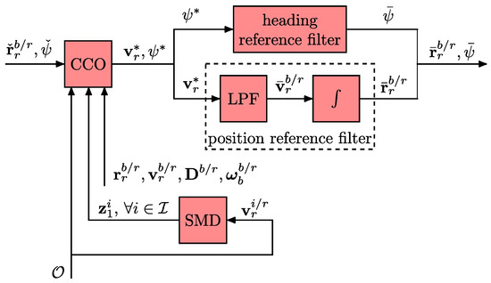
Figure 4. Block diagram of the proposed guidance strategy.

The heading reference filter consists of a hth-order overdamped LPF to guarantee the necessary smoothness of $\overline{\psi }$ and ensure that it has no overshoot with respect to the input ${\psi }^{*}$. This reference filter can be represented by the state-space model

$${\dot{\mathbf{y}}}_{\psi }=\mathbf{E}{\mathbf{y}}_{\psi }+\mathbf{F}{\psi }^{*},$$

(45)

where ${\mathbf{y}}_{\psi }\triangleq \left(\overline{\psi },\dot{\overline{\psi }},\dots ,{\overline{\psi }}^{(h-1)}\right)\in {\mathbb{R}}^h$, $\mathbf{F}\triangleq \left({\mathbf{0}}_{h-1},{\tau }_{\psi }^{-h}\right)\in {\mathbb{R}}^h$, ${\tau }_{\psi }\in {\mathbb{R}}_{>0}$ is a time constant, and

$$\begin{array}{cc}\hfill \mathbf{E}& \triangleq \left[\begin{array}{c}\begin{array}{cc}{\mathbf{0}}_{h-1\times 1}& {\mathbf{I}}_{h-1}\end{array}\\ E_1{E}_2\dots E_h\end{array}\right]\in {\mathbb{R}}^{h\times h},\hfill \\ \hfill E_{k+1}& \triangleq -\frac{h!}{k!(h-k)!}{\tau }_{\psi }^{-(h-k)},\forall k\in \{0,1,\dots ,h-1\}.\hfill \end{array}$$

The initial heading and heading rate commands are set equal to the respective MAV initial conditions, while the remaining filter states are set equal to zero, i.e.,

$${\mathbf{y}}_{\psi }\left(0\right)\triangleq \left(\psi \left(0\right),\dot{\psi }\left(0\right),0,\dots ,0\right).$$

(46)

It is worth noting that the target heading ${\psi }^{*}\left(t\right)$ given by the CCO may be discontinuous [16]. Then, designing the heading reference filter using an LPF of order h guarantees that $\overline{\psi }$ is minimally $(h-1)$-times differentiable with respect to time and has a Lipschitz-continuous first-time derivative. As a result, the smoothness requirement for $\overline{\psi }$ can be satisfied.

Similarly, to guarantee the necessary smoothness of ${\dot{\overline{\mathbf{v}}}}_r^{b/r}$, the position reference filter is designed using an overdamped LPF of order $h+1$ and an integrator, being represented by the state-space model

$${\dot{\mathbf{y}}}_p=\mathbf{A}{\mathbf{y}}_p+\mathbf{B}{\mathbf{v}}_r^{*},$$

(47)

where ${\mathbf{y}}_p\triangleq \left({\overline{\mathbf{r}}}_r^{b/r},{\dot{\overline{\mathbf{r}}}}_r^{b/r},\dots ,{\overline{\mathbf{r}}}_r^{b/r(h+1)}\right)\in {\mathbb{R}}^{3(h+2)}$,

$$\mathbf{B}\triangleq {\left[{\mathbf{0}}_{3\times 3(h+1)}{\mathbf{I}}_3{\tau }_p^{-(h+1)}\right]}^{\mathrm{T}}\in {\mathbb{R}}^{3(h+2)\times 3},$$

${\tau }_p\in {\mathbb{R}}_{>0}$ is a time constant, and

$$\begin{array}{cc}\hfill \mathbf{A}& \triangleq \left[\begin{array}{cc}{\mathbf{0}}_{3(h+1)\times 3}& {\mathbf{I}}_{3(h+1)}\\ {\mathbf{0}}_{3\times 3}& {\mathbf{A}}_1{\mathbf{A}}_2\dots {\mathbf{A}}_{h+1}\end{array}\right]\in {\mathbb{R}}^{3(h+2)\times 3(h+2)},\hfill \\ \hfill {\mathbf{A}}_{k+1}& \triangleq -\frac{(h+1)!}{k!(h+1-k)!}{\mathbf{I}}_3{\tau }_p^{-(h+1-k)},k\in \{0,1,\dots ,h\}.\hfill \end{array}$$

The initial position and velocity commands are set equal to the corresponding MAV initial conditions, while the remaining states of the filter are set equal to zero, i.e.,

$${\mathbf{y}}_p\left(0\right)\triangleq \left({\mathbf{r}}_r^{b/r}\left(0\right),{\mathbf{v}}_r^{b/r}\left(0\right),{\mathbf{0}}_3,\dots ,{\mathbf{0}}_3\right).$$

(48)

Analogous to ${\psi }^{*}$, the target velocity ${\mathbf{v}}_r^{*}\left(t\right)$ calculated by the CCO may be discontinuous [16]. Then, by using an LPF of order $h+1$, we guarantee that the acceleration command ${\dot{\overline{\mathbf{v}}}}_r^{b/r}$ is minimally ($h-1$)-times differentiable with respect to time and has a Lipschitz-continuous first-time derivative. As a result, the smoothness requirement of ${\dot{\overline{\mathbf{v}}}}_r^{b/r}$ is satisfied.

From the choice of ${\mathbf{y}}_p\left(0\right)$, we have that $\tilde{\mathbf{r}}\left(0\right)={\mathbf{0}}_3$ and $\tilde{\mathbf{v}}\left(0\right)={\mathbf{0}}_3$. Therefore, by properly designing the position control law (32), $\tilde{\mathbf{r}}$ and $\tilde{\mathbf{v}}$ can be limited, respectively, as

$$\begin{array}{cc}\hfill \parallel \tilde{\mathbf{r}}\left(t\right)\parallel & \le {ϵ}^r,\hfill \end{array}$$

(49)

$$\begin{array}{cc}\hfill \parallel \tilde{\mathbf{v}}\left(t\right)\parallel & \le {ϵ}^v,\hfill \end{array}$$

(50)

where ${ϵ}^r\in {\mathbb{R}}_{\ge 0}$ and ${ϵ}^v\in {\mathbb{R}}_{\ge 0}$ can be chosen as time-dependent functions. It is worth noting that ${ϵ}^r$ and ${ϵ}^v$ cannot be analytically calculated, but they can be approximated from numerical simulations of the position closed-loop system (30) and (37) using a great amount of values of the disturbance force inside the bounds provided in Assumption 4.

Assume that obstacle i and the MAV can be contained, respectively, in the closed spheres $\mathcal{B}\left(C_i,{\rho }_i\right)$ and $\mathcal{B}\left(B,{\rho }_b\right)$, where ${\rho }_i\in {\mathbb{R}}_{>0}$ and ${\rho }_b\in {\mathbb{R}}_{>0}$ are of a given radius. Therefore, a collision between the MAV and obstacle i is assumed to take place if and only if

$$∥{\mathbf{r}}_r^{b/r}\left(t\right)-{\mathbf{r}}_r^{i/r}\left(t\right)∥\le {\rho }_{bi},$$

(51)

where ${\rho }_{bi}\triangleq {\rho }_b+{\rho }_i$.

Using the position error bound (49) and the position error definition (28), condition (51) can be tightened to obtain

$$∥{\overline{\mathbf{r}}}_r^{b/r}\left(t\right)-{\mathbf{r}}_r^{i/r}\left(t\right)∥\le {\rho }_{bi}+{ϵ}^r,$$

(52)

whose satisfaction implies that condition (51) is true.

To prevent collisions, the adopted strategy is to avoid satisfying (52) in a future time horizon of finite length $\tau \in {\mathbb{R}}_{>0}$. To this end, we must predict ${\overline{\mathbf{r}}}_r^{b/r}\left(t\right)$ and ${\mathbf{r}}_r^{i/r}\left(t\right)$ inside the time interval $[t_0,t_0+\tau ]$, where $t_0\in {\mathbb{R}}_{\ge 0}$ is the current time. By using the length $\tau$, we only consider the obstacles that can cause imminent collisions, i.e., collisions that can occur inside $[t_0,t_0+\tau ]$. This can be effective to reduce the computational burden when there are many obstacles. However, the parameter $\tau$ must be chosen based on the physical bounds of the obstacles’ trajectories and the MAV dynamics in such a way that the MAV can avoid a collision when it is detected as imminent.

From (47), one can see that the future values of ${\overline{\mathbf{r}}}_r^{b/r}$ are unknown once they depend on the future values of ${\mathbf{v}}_r^{*}$, which are calculated in real time by the CCO and dependent on the unknown future behavior of the obstacles. In this context, we predict ${\overline{\mathbf{r}}}_r^{b/r}$ on the time interval $[t_0,t_0+\tau ]$ by considering ${\mathbf{v}}_r^{*}$ as a constant. Therefore, to support the forthcoming derivations, Lemma 3 provides a unique solution to (47) with a given initial condition ${\mathbf{y}}_p\left(t_0\right)$, while considering ${\mathbf{v}}_r^{*}$ as a constant.

Lemma 3. 

Considering ${\mathit{v}}_r^{*}$ as a constant input, the solution of (47) in $t\in [t_0,\infty )$ with initial condition ${\mathit{y}}_p\left(t_0\right)$ is given by

$${\mathit{y}}_p\left(t\right)=e^{\mathit{A}\delta t}{\mathit{y}}_p\left(t_0\right)+\mathit{G}\left(\delta t\right){\mathit{v}}_r^{*},$$

(53)

where $\delta t\triangleq t-t_0$,

$$\mathit{G}\left(\delta t\right)\triangleq \left[{\mathit{I}}_{3(h+2)}{\mathbf{0}}_{3(h+2)\times 3}\right]e^{\overline{\mathit{A}}\delta t}{\left[{\mathbf{0}}_{3\times 3(h+2)}{\mathit{I}}_3\right]}^{\mathrm{T}},$$

$$\overline{\mathit{A}}\triangleq \left[\begin{array}{cc}\mathit{A}& \mathit{B}\\ {\mathbf{0}}_{3\times 3(h+2)}& {\mathbf{0}}_{3\times 3}\end{array}\right]\in {\mathbb{R}}^{3(h+3)\times 3(h+3)}.$$

Proof. 

See Appendix A.    □

Considering ${\mathbf{v}}_r^{*}$ as a constant input, the predicted values of the MAV position command ${\overline{\mathbf{r}}}_r^{b/r}\left(t\right)$, which we denote by ${\widehat{\overline{\mathbf{r}}}}_r^{b/r}\left(t\right)\in {\mathbb{R}}^3$, can be obtained from (53) as

$$\begin{array}{cc}\hfill {\widehat{\overline{\mathbf{r}}}}_r^{b/r}\left(t\right)& ={\mathbf{C}}_1{e}^{\mathbf{A}\delta t}{\mathbf{y}}_p\left(t_0\right)+{\mathbf{G}}_1\left(\delta t\right){\mathbf{v}}_r^{*},\hfill \end{array}$$

(54)

where ${\mathbf{G}}_1\left(\delta t\right)\triangleq {\mathbf{C}}_1\mathbf{G}\left(\delta t\right)$ and ${\mathbf{C}}_1\triangleq \left[{\mathbf{I}}_3{\mathbf{0}}_{3\times 3(h+1)}\right]\in {\mathbb{R}}^{3\times 3(h+2)}$.

The earlier VO-based approaches generally assume that the obstacles keep a constant velocity. In practice, however, this assumption only ensures collision avoidance against obstacles with low acceleration capacity or under a large $\mathit{\tau }$. Here, instead of predicting the obstacles’ trajectories using a first-order approximation, we consider a set of possible future trajectories for the obstacles based on estimates of their acceleration bounds calculated from ${\mathbf{z}}_1^i$ provided by the SMD. In this context, the predicted position ${\widehat{\mathbf{r}}}_r^{i/r}\in {\mathbb{R}}^3$ of obstacle i inside the time interval $[t_0,t_0+\tau ]$ belongs to

$$\begin{array}{cc}\hfill {\mathcal{R}}_i\triangleq & \left\{\mathbf{r}\left(t\right)={\mathbf{r}}_r^{i/r}\left(t_0\right)+\delta t{\mathbf{v}}_r^{i/r}\left(t_0\right)+{\widehat{a}}_i^{\max }\mathit{\vartheta }\frac{\delta t^2}{2},\delta t\in [0,\mathit{\tau }],\mathit{\vartheta }\in \mathcal{B}\left({\mathbf{0}}_3,1\right)\right\},\hfill \end{array}$$

(55)

where ${\widehat{a}}_i^{\max }\in {\mathbb{R}}_{\ge 0}$ is a bound estimate of obstacle i acceleration.

Let ${\mathbf{v}}_r^{i/r}$ be n-times differentiable with respect to time, where $n\ge 1$, such that ${\mathbf{v}}_r^{i/r\left(n\right)}$ has a known Lipschitz constant vector ${\gamma }_i>{\mathbf{0}}_3$. Define a vector $\gamma \in {\mathbb{R}}^3$ such that $\gamma >{\gamma }_i,$$\forall i\in \mathcal{I}$. To estimate the obstacle i acceleration, we use the high-order SMD [11,31]

$$\left\{\begin{array}{c}{\dot{\mathbf{z}}}_0^i={\mathbf{w}}_0^i,\hfill \\ {\mathbf{w}}_0^i=-{\mathbf{\Lambda }}_0\mathbf{\Psi }{\left(\gamma \right)}^{1/(n+1)}\mathbf{\Psi }\left(\right|{\mathbf{z}}_0^i-{\mathbf{v}}_r^{i/r}{\left|\right)}^{n/(n+1)}\mathrm{sign}({\mathbf{z}}_0^i-{\mathbf{v}}_r^{i/r})+{\mathbf{z}}_1^i,\hfill \\ {\dot{\mathbf{z}}}_1^i={\mathbf{w}}_1^i,\hfill \\ {\mathbf{w}}_1^i=-{\mathbf{\Lambda }}_1\mathbf{\Psi }{\left(\gamma \right)}^{1/n}\mathbf{\Psi }\left(\right|{\mathit{\eta }}_1^i{\left|\right)}^{(n-1)/n}\mathrm{sign}\left({\mathit{\eta }}_1^i\right)+{\mathbf{z}}_2^i,\hfill \\ ⋮\hfill \\ {\dot{\mathbf{z}}}_{n-1}^i={\mathbf{w}}_{n-1}^i,\hfill \\ {\mathbf{w}}_{n-1}^i=-{\mathbf{\Lambda }}_{n-1}\mathbf{\Psi }{\left(\gamma \right)}^{1/2}\mathbf{\Psi }\left(\right|{\mathit{\eta }}_{n-1}^i{\left|\right)}^{1/2}\mathrm{sign}\left({\mathit{\eta }}_{n-1}^i\right)+{\mathbf{z}}_n^i,\hfill \\ {\dot{\mathbf{z}}}_n^i=-{\mathbf{\Lambda }}_n\mathbf{\Psi }\left(\gamma \right)\mathrm{sign}\left({\mathit{\eta }}_n^i\right),\hfill \end{array}\right.$$

(56)

where ${\mathit{\eta }}_k^i\triangleq {\mathbf{z}}_k^i-{\mathbf{w}}_{k-1}^i$, with $k\in \{1,\dots ,n\}$; ${\mathbf{\Lambda }}_j\in {\mathbb{R}}^{3\times 3}$ is a positive-definite diagonal matrix, with $j\in \left\{0,\dots ,n\right\}$; and $\mathbf{\Psi }\left(\right|·\left|\right)\triangleq \mathrm{diag}\left(\right|·\left|\right)$ maps a vector into a diagonal matrix. The SMD (56) initial conditions are set to ${\mathbf{z}}_0^i\left(0\right)={\mathbf{v}}_r^{i/r}\left(0\right)$ and ${\mathbf{z}}_j^i\left(0\right)={\mathbf{0}}_3$, $\forall j\in \{1,\dots ,n\}$.

Lemma 4 

([31]). Consider the SMD (56). For any ${\mathbf{\Lambda }}_n$ satisfying

$$\begin{array}{c}\hfill {\mathbf{\Lambda }}_n{\mathbf{1}}_3>{\mathbf{1}}_3,\end{array}$$

there exists a set of positive-definite diagonal matrices $\{{\mathbf{\Lambda }}_0,\dots ,{\mathbf{\Lambda }}_{n-1}\}$ that provides the finite-time convergence of ${\mathit{z}}_k^i$ to ${\mathit{v}}_i^{\left(k\right)}$, $\forall k\in \left\{0,\dots ,n\right\}$ and $\forall i\in \mathcal{I}$.

Note that, before the differentiator (56)’s convergence time, denoted by $t_c^i\in {\mathbb{R}}_{>0}$, there is no accurate information about the acceleration bound of obstacle i. In this context, we choose to calculate ${\widehat{a}}_i^{\max }$ as

$${\widehat{a}}_i^{\max }\left(t\right)\triangleq \left\{\begin{array}{cc}\underset{t_c^i\le \delta \le t}{\max }\parallel {\mathbf{z}}_1^i\left(\delta \right)\parallel \hfill & \forall t\ge t_c^i,\hfill \\ \parallel {\mathbf{z}}_1^i\left(t\right)\parallel \hfill & \forall t<t_c^i.\hfill \end{array}\right.$$

(57)

According to (57), before $t_c^i$, ${\widehat{a}}_i^{\max }$ is converging according to the SMD (56), and after $t_c^i$, by maximizing $\parallel {\mathbf{z}}_1^i\parallel$ over the time interval $[t_c^i,t]$, ${\widehat{a}}_i^{\max }$ becomes an accurate estimate of obstacle i’s acceleration bound inside the considered time interval. However, since $t_c^i$ is difficult to calculate without conservativeness, a very intuitive choice to approximate it is by verifying when the SMD states enter a small neighborhood of the sliding manifold, i.e., when

$$\parallel {\mathbf{z}}_0^i-{\mathbf{v}}_r^{i/r}\parallel +\parallel {\mathit{\eta }}_1^i\parallel +\cdots +\parallel {\mathit{\eta }}_n^i\parallel <\alpha ,$$

(58)

where $\alpha \in {\mathbb{R}}_{>0}$ is satisfied.

Using ${\widehat{\overline{\mathbf{r}}}}_r^{b/r}\left(t\right)$ and ${\widehat{\mathbf{r}}}_r^{i/r}\left(t\right)$ given, respectively, by (54) and (55), the collision condition (52) can be further tightened to obtain

$$∥{\mathbf{G}}_1\left(\delta t\right){\mathbf{v}}_r^{*}-{\mathbf{c}}_i\left(\delta t\right)-{\widehat{a}}_i^{\max }\mathit{\vartheta }\frac{\delta t^2}{2}∥\le {\rho }_{bi}+{ϵ}^r,$$

(59)

where ${\mathbf{c}}_i\left(\delta t\right)\triangleq -{\mathbf{C}}_1{e}^{\mathbf{A}\delta t}{\mathbf{y}}_p\left(t_0\right)+{\mathbf{r}}_r^{i/r}\left(t_0\right)+\delta t{\mathbf{v}}_r^{i/r}\left(t_0\right)$. In turn, we can also notice that the collision condition (59) is always satisfied if

$$∥{\mathbf{G}}_1\left(\delta t\right){\mathbf{v}}_r^{*}-{\mathbf{c}}_i\left(\delta t\right)∥\le {\rho }_{bi}^{+}\left(\delta t\right),$$

(60)

where ${\rho }_{bi}^{+}\left(\delta t\right)\triangleq {\rho }_{bi}+{ϵ}^r+{\widehat{a}}_i^{\max }\frac{\delta t^2}{2}$.

From the definition of ${\mathbf{G}}_1\left(\delta t\right)$, one can see that it is nonsingular $\forall \delta t>0$. Then, by multiplying both sides of (60) by $\parallel {\mathbf{G}}_1^{-1}\left(\delta t\right)\parallel$, it can be shown that (60) is satisfied if

$$∥{\mathbf{v}}_r^{*}-{\mathbf{G}}_1^{-1}\left(\delta t\right){\mathbf{c}}_i\left(\delta t\right)∥\le \parallel {\mathbf{G}}_1^{-1}\left(\delta t\right)\parallel {\rho }_{bi}^{+}\left(\delta t\right).$$

(61)

Now, using (61), define a set of target velocities ${\mathbf{v}}_r^{*}$ that may result in a collision with obstacle i within $(t_0,t_0+\tau ]$ as

$${\mathcal{CCO}}_{bi}^{\tau }\triangleq \bigcup _{0<\delta t\le \tau }\mathcal{B}\left({\mathbf{G}}_1^{-1}\left(\delta t\right){\mathbf{c}}_i\left(\delta t\right),\parallel {\mathbf{G}}_1^{-1}\left(\delta t\right)\parallel {\rho }_{bi}^{+}\left(\delta t\right)\right).$$

Therefore, the set of target velocities ${\mathbf{v}}_r^{*}$ that may result in a collision with any obstacle within $(t_0,t_0+\tau ]$ is given by

$${\mathcal{CCO}}_b^{\tau }\triangleq \bigcup _{\forall i\in \mathcal{I}}{\mathcal{CCO}}_{bi}^{\tau }.$$

In other words, we can guarantee collision avoidance against accelerated obstacles by merely continuously choosing ${\mathbf{v}}_r^{*}\notin {\mathcal{CCO}}_b^{\tau }$, thus satisfying the position constraint (9).

To consider the linear velocity constraint (10), we can rewrite it in terms of the target velocity ${\mathbf{v}}_r^{*}$. To this end, note that, given the choice of ${\mathbf{y}}_p\left(0\right)$ in (48) and the design of the position reference filter (47) using the adopted overdamped LPF, ${\overline{\mathbf{v}}}_r^{b/r}$ presents no overshoot relative to the input ${\mathbf{v}}_r^{*}$. Consequently, by choosing ${\mathbf{v}}_r^{*}\in \mathcal{V}$, we guarantee that ${\overline{\mathbf{v}}}_r^{b/r}\in \mathcal{V}$ since $\mathcal{V}$ is a convex set. Then, from the velocity tracking error definition (29) and bound (50), one can see that by choosing

$${\mathbf{v}}_r^{*}\in \mathcal{V}\ominus \mathcal{B}\left({\mathbf{0}}_3,{ϵ}^v\right),$$

(62)

it holds that ${\mathbf{v}}_r^{b/r}\in \mathcal{V}$, thus respecting the velocity constraint (10). Then, the position and velocity constraints (9) and (10) can be respected by continuously choosing

$${\mathbf{v}}_r^{*}\in {\mathcal{V}}_{\mathrm{R}}\triangleq \left(\mathcal{V}\ominus \mathcal{B}\left({\mathbf{0}}_3,{ϵ}^v\right)\right)\setminus {\mathcal{CCO}}_b^{\tau }.$$

(63)

It should be noted that the set ${\mathcal{V}}_{\mathrm{R}}$ is generally non-convex.

On the other hand, to account for the rotor thrust constraint (11), it can be seen from the control allocation Equation (8) and Assumption 1 that (11) results in the following control command constraints:

$$\left[\begin{array}{c}\overline{f}\\ {\overline{\mathit{\tau }}}_b^c\end{array}\right]\in \mathcal{U},$$

(64)

where $\mathcal{U}\triangleq \left\{\mathit{\nu }\in {\mathbb{R}}^{n_r}|\mathit{\nu }=\mathbf{\Gamma }{\mathbf{f}}^r,{\mathbf{f}}^r\in \mathcal{F}\right\}$.

Knowing that $\overline{f}=\parallel {\overline{\mathbf{f}}}_r^c\parallel$ and the attitude control loop has an integral sliding mode, i.e., ${\mathbf{D}}^{b/r}\equiv {\overline{\mathbf{D}}}^{b/r}$ and ${\mathit{\omega }}_b^{b/r}\equiv {\overline{\mathit{\omega }}}_b^{b/r}$, by substituting the control torque command (23) and the control force command (32) into (64), we obtain

$$\left[\begin{array}{c}∥g{\mathbf{e}}_3+{\dot{\overline{\mathbf{v}}}}_r^{b/r}-{\mathbf{K}}_2\tilde{\mathbf{r}}-{\mathbf{K}}_3\tilde{\mathbf{v}}-m^{-1}{\widehat{\mathbf{f}}}_r^d∥\\ {\dot{\overline{\mathit{\omega }}}}_b^{b/r}-{\mathbf{J}}_b^{-1}\left[{\mathbf{J}}_b{\overline{\mathit{\omega }}}_b^{b/r}\times \right]{\overline{\mathit{\omega }}}_b^{b/r}-2{\mathbf{K}}_1\mathrm{sign}\left(\mathbf{s}\right)\end{array}\right]\in \mathbf{H}\mathcal{U},$$

(65)

where

$$\mathbf{H}\triangleq \left[\begin{array}{cc}{m}^{-1}& {\mathbf{0}}_{1\times 3}\\ {\mathbf{0}}_{3\times 3}& {\mathbf{J}}_b^{-1}\end{array}\right].$$

To respect the rotor thrust constraint (11), our strategy is to guarantee the satisfaction of (65) in the time horizon $\mathit{\tau }$. To this end, we have to predict the left side of (65). However, note that we cannot predict the terms ${\mathbf{K}}_2\tilde{\mathbf{r}}$, ${\mathbf{K}}_3\tilde{\mathbf{v}}$, and ${\widehat{\mathbf{f}}}_r^d$. In this sense, using the tracking error bounds (49) and (50), Assumption 4, and the definition of $\mathrm{sign}\left(\mathbf{s}\right)$, condition (65) can be tightened to obtain

$$\left[\begin{array}{c}∥{\dot{\overline{\mathbf{v}}}}_r^{b/r}+g{\mathbf{e}}_3∥\\ {\dot{\overline{\mathit{\omega }}}}_b^{b/r}-{\mathbf{J}}_b^{-1}\left[{\mathbf{J}}_b{\overline{\mathit{\omega }}}_b^{b/r}\times \right]{\overline{\mathit{\omega }}}_b^{b/r}\end{array}\right]\in \mathbf{H}\mathcal{U}\ominus \left[\begin{array}{c}\Delta \mathcal{F}\\ {\mathcal{K}}_1\end{array}\right]$$

(66)

where ${\mathcal{K}}_1\triangleq \left\{\gamma \in {\mathbb{R}}^3\left|\right|\gamma |=2{\mathbf{K}}_1{\mathbf{1}}_3\right\}$ and

$$\begin{array}{cc}\hfill \Delta \mathcal{F}& \triangleq \left\{x\in \mathbb{R}\left|\right|x|\le \parallel {\mathbf{K}}_2\parallel {ϵ}^r+\parallel {\mathbf{K}}_3\parallel {ϵ}^v+m^{-1}\parallel {\mathbf{f}}^{\max }\parallel \right\}.\hfill \end{array}$$

A prediction for ${\dot{\overline{\mathbf{v}}}}_r^{b/r}$ inside the time interval $\left[t_0,t_0+\mathit{\tau }\right]$ can be directly obtained from (53). On the other hand, a prediction for ${\overline{\mathit{\omega }}}_b^{b/r}$ cannot be exactly obtained. To support this statement, note that for the considered class of underactuated MAVs, the angular velocity command is given by

$${\overline{\mathit{\omega }}}_b^{b/r}={\mathbf{e}}_3\times {\overline{\mathbf{D}}}^{b/r}{\dot{\overline{\mathbf{n}}}}_r+\dot{\overline{\psi }}{\mathbf{e}}_3.$$

(67)

Then, note that ${\overline{\mathbf{D}}}^{b/r}$ depends on ${\overline{\mathbf{n}}}_r$ (see (25)–(27)), which is a unit vector that has the same direction and orientation of the control force command ${\overline{\mathbf{f}}}_r^c$ (see (12)). However, it can be seen from (32) that ${\overline{\mathbf{f}}}_r^c$ cannot be exactly predicted since the future values of the terms ${\mathbf{K}}_2\tilde{\mathbf{r}}$, ${\mathbf{K}}_3\tilde{\mathbf{v}}$, and ${\widehat{\mathbf{f}}}_r^d$ are unknown. As a result, we cannot obtain an exact prediction for ${\overline{\mathit{\omega }}}_b^{b/r}$ inside $[t_0,t_0+\tau ]$.

On the basis of the above discussion, ${\overline{\mathbf{n}}}_r$ can be rewritten in terms of a nominal part ${\overline{\mathbf{n}}}_r^n\in {\mathbb{R}}^3$ and an unknown part $\Delta {\overline{\mathbf{n}}}_r\in {\mathbb{R}}^3$, i.e.,

$${\overline{\mathbf{n}}}_r={\overline{\mathbf{n}}}_r^n+\Delta {\overline{\mathbf{n}}}_r,$$

(68)

where ${\overline{\mathbf{n}}}_r^n\triangleq \frac{{\dot{\overline{\mathbf{v}}}}_r^{b/r}+g{\mathbf{e}}_3}{\parallel {\dot{\overline{\mathbf{v}}}}_r^{b/r}+g{\mathbf{e}}_3\parallel }.$

Using (68), Equation (67) can be rewritten as

$${\overline{\mathit{\omega }}}_b^{b/r}={\overline{\mathit{\omega }}}_b^n+\Delta {\overline{\mathit{\omega }}}_b,$$

(69)

where ${\overline{\mathit{\omega }}}_b^n\triangleq {\mathbf{e}}_3\times {\overline{\mathbf{D}}}^{b/r,n}{\dot{\overline{\mathbf{n}}}}_r^n+\dot{\overline{\psi }}{\mathbf{e}}_3$, being ${\overline{\mathbf{D}}}^{b/r,n}$ calculated in the same way as ${\overline{\mathbf{D}}}^{b/r}$ in (25) but considering ${\overline{\mathbf{n}}}_r^n$ instead of ${\overline{\mathbf{n}}}_r$, and $\Delta {\overline{\mathit{\omega }}}_b\in {\mathbb{R}}^3$ is an unknown part.

Substituting (69), condition (66) can be rewritten as

$$\left[\begin{array}{c}∥{\dot{\overline{\mathbf{v}}}}_r^{b/r}+g{\mathbf{e}}_3∥\\ {\dot{\overline{\mathit{\omega }}}}_b^n-{\mathbf{J}}_b^{-1}\left[{\mathbf{J}}_b{\overline{\mathit{\omega }}}_b^n\times \right]{\overline{\mathit{\omega }}}_b^n+\delta \overline{\mathit{\omega }}\end{array}\right]\in \mathbf{H}\mathcal{U}\ominus \left[\begin{array}{c}\Delta \mathcal{F}\\ {\mathcal{K}}_1\end{array}\right],$$

(70)

where

$$\delta \overline{\mathit{\omega }}\triangleq \Delta {\dot{\overline{\mathit{\omega }}}}_b-{\mathbf{J}}_b^{-1}\left[{\mathbf{J}}_b\Delta {\overline{\mathit{\omega }}}_b\times \right]{\overline{\mathit{\omega }}}_b^{b/r}-{\mathbf{J}}_b^{-1}\left[{\mathbf{J}}_b{\overline{\mathit{\omega }}}_b^n\times \right]\Delta {\overline{\mathit{\omega }}}_b.$$

Considering that $\delta \overline{\mathit{\omega }}\in \Delta \overline{\mathcal{W}}$, condition (70) can be tightened one last time to obtain

$$\left[\begin{array}{c}∥{\dot{\overline{\mathbf{v}}}}_r^{b/r}+g{\mathbf{e}}_3∥\\ {\dot{\overline{\mathit{\omega }}}}_b^n-{\mathbf{J}}_b^{-1}\left[{\mathbf{J}}_b{\overline{\mathit{\omega }}}_b^n\times \right]{\overline{\mathit{\omega }}}_b^n\end{array}\right]\in \mathbf{H}\mathcal{U}\ominus \Delta \mathcal{U},$$

(71)

where

$$\Delta \mathcal{U}\triangleq \left[\begin{array}{c}\Delta \mathcal{F}\\ {\mathcal{K}}_1\oplus \Delta \overline{\mathcal{W}}\end{array}\right].$$

Regarding the set $\Delta \overline{\mathcal{W}}$, consider the following remark.

Remark 3. 

An analytic expression for $\Delta {\overline{\mathit{\omega }}}_b$ is difficult to obtain since the relation between ${\overline{\mathit{D}}}^{b/r}$ and ${\overline{\mathit{n}}}_r$ is strongly nonlinear (see (25)–(27)). Consequently, it is complex to obtain an analytical expression for the set $\Delta \overline{\mathcal{W}}$. Therefore, we approximate it based on computer simulations.

Now, we are able to predict the left side of (71) inside the time interval $[t_0,t_0+\mathit{\tau }]$. In this sense, let us rewrite (71) in terms of the predicted values for each variable, i.e.,

$$\left[\begin{array}{c}∥{\widehat{\overline{\mathbf{a}}}}_r^{b/r}+g{\mathbf{e}}_3∥\\ {\dot{\widehat{\overline{\mathit{\omega }}}}}_b^n-{\mathbf{J}}_b^{-1}\left[{\mathbf{J}}_b{\widehat{\overline{\mathit{\omega }}}}_b^n\times \right]{\widehat{\overline{\mathit{\omega }}}}_b^n\end{array}\right]\in \mathbf{H}\mathcal{U}\ominus \Delta \mathcal{U},$$

(72)

where ${\widehat{\overline{\mathbf{a}}}}_r^{b/r}\in {\mathbb{R}}^3$ and ${\widehat{\overline{\mathit{\omega }}}}_b^n\in {\mathbb{R}}^3$ are, respectively, the predictions of ${\dot{\overline{\mathbf{v}}}}_r^{b/r}$ and ${\overline{\mathit{\omega }}}_b^n$ inside $[t_0,t_0+\tau ]$.

The acceleration command prediction ${\widehat{\overline{\mathbf{a}}}}_r^{b/r}$ can be obtained from (53) using the same strategy adopted to predict the position command ${\overline{\mathbf{r}}}_r^{b/r}\left(t\right)$, i.e., considering ${\mathbf{v}}_r^{*}$ as a constant input inside the time interval $[t_0,t_0+\tau ]$, yielding

$$\begin{array}{cc}\hfill {\widehat{\overline{\mathbf{a}}}}_r^{b/r}\left(t\right)& ={\mathbf{C}}_3{e}^{\mathbf{A}\delta t}{\mathbf{y}}_p\left(t_0\right)+{\mathbf{G}}_3\left(\delta t\right){\mathbf{v}}_r^{*},\hfill \end{array}$$

(73)

where ${\mathbf{G}}_3\left(\delta t\right)\triangleq {\mathbf{C}}_3\mathbf{G}\left(\delta t\right)$ and ${\mathbf{C}}_3\triangleq \left[{\mathbf{0}}_{3\times 6}{\mathbf{I}}_3{\mathbf{0}}_{3\times 3(h-1)}\right]\in {\mathbb{R}}^{3\times 3(h+2)}$.

On the other hand, note that the angular velocity prediction ${\widehat{\overline{\mathit{\omega }}}}_b^n$ can be calculated by differentiating ${\overline{\mathbf{D}}}^{b/r,n}$ with respect to time. Here, we choose to predict ${\overline{\mathbf{D}}}^{b/r,n}\left(t\right)$ inside the interval $[t_0,t_0+\tau ]$ using the Euler angles 1-2-3 parameterization, denoted by ${\widehat{\overline{\mathit{\alpha }}}}^{b/r}\left(t\right)\triangleq (\widehat{\overline{\varphi }}\left(t\right),\widehat{\overline{\theta }}\left(t\right),\widehat{\overline{\psi }}\left(t\right))$. The prediction of the heading command $\widehat{\overline{\psi }}$ is obtained by adopting the same strategy used to predict ${\overline{\mathbf{r}}}_r^{b/r}\left(t\right)$ and ${\dot{\overline{\mathbf{v}}}}_r^{b/r}\left(t\right)$, i.e., considering ${\psi }^{*}$ as a constant input. Under this assumption, $\widehat{\overline{\psi }}\left(t\right)$ can be calculated from the actual time instant $t_0$ by solving Equation (45), yielding

$$\begin{array}{cc}\hfill \widehat{\overline{\psi }}\left(t\right)& ={\mathbf{C}}_1^{\psi }{e}^{\mathbf{E}\delta t}{\mathbf{y}}_{\psi }\left(t_0\right)+{\mathbf{C}}_1^{\psi }{\mathbf{E}}^{-1}\left(e^{\mathbf{E}\delta t}-{\mathbf{I}}_h\right)\mathbf{F}{\psi }^{*},\hfill \end{array}$$

(74)

where ${\mathbf{C}}_1^{\psi }\triangleq \left(1,{\mathbf{0}}_{1\times (h-1)}\right)$.

The predictions $\widehat{\overline{\varphi }}$ and $\widehat{\overline{\theta }}$ inside $[t_0,t_0+\tau ]$ can be obtained from Equations (26) and (27) and the definition of ${\overline{\mathbf{n}}}_r^n$ given after (68), being given by

$$\begin{array}{cc}\hfill \widehat{\overline{\varphi }}& =-{tan}^{-1}\frac{{\mathbf{e}}_2^{\mathrm{T}}{\widehat{\overline{\mathbf{n}}}}_r^n}{{\mathbf{e}}_3^{\mathrm{T}}{\widehat{\overline{\mathbf{n}}}}_r^n},\hfill \\ \hfill \widehat{\overline{\theta }}& ={\sin }^{-1}\left({\mathbf{e}}_1^{\mathrm{T}}{\widehat{\overline{\mathbf{n}}}}_r^n\right),\hfill \end{array}$$

where

$${\widehat{\overline{\mathbf{n}}}}_r^n=\frac{{\widehat{\overline{\mathbf{a}}}}_r^{b/r}+g{\mathbf{e}}_3}{\parallel {\widehat{\overline{\mathbf{a}}}}_r^{b/r}+g{\mathbf{e}}_3\parallel },$$

being ${\widehat{\overline{\mathbf{a}}}}_r^{b/r}$ the acceleration command prediction defined in Equation (73). Then, the angular velocity prediction ${\widehat{\overline{\mathit{\omega }}}}_b^n$ can be immediately calculated by

$${\widehat{\overline{\mathit{\omega }}}}_b^n={\mathbf{A}}_{\alpha }{\dot{\widehat{\overline{\mathit{\alpha }}}}}^{b/r},$$

(75)

where

$${\mathbf{A}}_{\mathit{\alpha }}\triangleq \left[\begin{array}{ccc}\cos (\widehat{\overline{\theta }})\cos (\widehat{\overline{\psi }})& \sin (\widehat{\overline{\psi }})& 0\\ -\sin (\widehat{\overline{\psi }})\cos (\widehat{\overline{\theta }})& \cos (\widehat{\overline{\psi }})& 0\\ \sin (\widehat{\overline{\theta }})& 0& 1\end{array}\right].$$

The angular acceleration prediction ${\dot{\widehat{\overline{\mathit{\omega }}}}}_b^n$ is simply obtained by differentiating (75) with respect to time.

The continuous selection of ${\mathbf{v}}_r^{*}$ and ${\psi }^{*}$ such that condition (72) is satisfied in $[t_0,t_0+\tau ]$ guarantees the satisfaction of the control command constraints (64) and, consequently, the rotor thrust constraint (11).

Lastly, to completely solve Problem 1, we formulate a bilevel optimization problem [41] that calculates ${\mathbf{v}}_r^{*}$ and ${\psi }^{*}$, giving priority to collision avoidance. In this sense, we compute ${\mathbf{v}}_r^{*}$ and ${\psi }^{*}$ as the solution of the following minimization that aims to satisfy the linear velocity and rotor thrust constraints, respectively, given by (10) and (11), and make the MAV reach its desired position ${\check{\mathbf{r}}}_r^{b/r}$ and desired heading $\check{\psi }$ without collision:

$$\begin{array}{cc}\hfill \left({\mathbf{v}}_r^{*},{\psi }^{*}\right)=\underset{\left(\mathit{\nu },\beta \right)}{\arg \min }& \parallel {\mathbf{v}}^{\mathrm{pref}}-\mathit{\nu }{\displaystyle \parallel }\hfill \\ \hfill \mathrm{s}.\mathrm{t}.& \mathit{\nu }\in {\mathcal{V}}_{\mathrm{R}},\hfill & \\ \hfill & \beta \in \mathcal{Z},\hfill \end{array}$$

(76)

where ${\mathbf{v}}^{\mathrm{pref}}\in {\mathbb{R}}^3$ is a preferred velocity and $\mathcal{Z}$ is the set of solutions to the $\mathit{\nu }$-parameterized problem

$$\begin{array}{cc}\hfill \underset{z\in (\pi ,\pi ]}{min}& |\check{\psi }-z|\hfill \\ \hfill \mathrm{s}.\mathrm{t}.& \widehat{\mathbf{U}}(t;\mathit{\nu },z)\in \mathbf{H}\mathcal{U}\ominus \Delta \mathcal{U},\forall t\in (t_0,t_0+\tau ],\hfill \end{array}$$

with

$$\widehat{\mathbf{U}}(t;\mathit{\nu },\beta )\triangleq \left[\begin{array}{c}∥{\widehat{\overline{\mathbf{a}}}}_r^{b/r}(t;\mathit{\nu })+g{\mathbf{e}}_3∥\\ {\dot{\widehat{\overline{\mathit{\omega }}}}}_b^n(t;\mathit{\nu },z)-{\mathbf{J}}_b^{-1}\left[{\mathbf{J}}_b{\widehat{\overline{\mathit{\omega }}}}_b^n(t;\mathit{\nu },z)\times \right]{\widehat{\overline{\mathit{\omega }}}}_b^n(t;\mathit{\nu },z)\end{array}\right].$$

Here, ${\mathbf{v}}^{\mathrm{pref}}$ is a vector that points to ${\check{\mathbf{r}}}_r^{b/r}$ and has a magnitude equal to the maximum admissible velocity in this direction. To provide a smooth deceleration phase, the magnitude of ${\mathbf{v}}^{\mathrm{pref}}$ is gradually decreased according to the remaining distance when the vehicle is near ${\check{\mathbf{r}}}_r^{b/r}$. However, we highlight that the design of ${\mathbf{v}}^{\mathrm{pref}}$ can be done using other strategies [26,42].

When obstacles are present, the set ${\mathcal{V}}_{\mathrm{R}}$ is generally non-convex and can even become empty in very dense scenarios. In this case, it is appropriate to choose a target velocity and heading that result in the largest time to collide, while respecting constraints (10) and (11). The shortest time for a collision to occur, denoted by $t_{\mathrm{col}}\in {\mathbb{R}}_{>0}$, as a result of choosing a certain target velocity $\mathit{\nu }$ is given by

$$\begin{array}{cc}\hfill t_{\mathrm{col}}\left(\mathit{\nu }\right)=\underset{0<\delta \le \mathit{\tau }}{min}& \delta \hfill \\ \hfill \mathrm{s}.\mathrm{t}.& \mathit{\nu }\in {\mathcal{CCO}}_b^{\delta }.\hfill \end{array}$$

Therefore, in case there is no solution to (76), i.e., ${\mathcal{V}}_{\mathrm{R}}=\varnothing$, we propose to choose the target velocity and heading that imply the largest $t_{\mathrm{col}}$, while respecting constraints (10) and (11), i.e.,

$$\begin{array}{cc}\hfill \left({\mathbf{v}}_r^{*},{\psi }^{*}\right)=\underset{\left(\mathit{\nu },\beta \right)}{\arg \max }& t_{\mathrm{col}}\left(\mathit{\nu }\right)\hfill \\ \hfill \mathrm{s}.\mathrm{t}.& \mathit{\nu }\in \mathcal{V}\ominus \mathcal{B}\left({\mathbf{0}}_3,{ϵ}^v\right),\hfill & \\ \hfill & \beta \in \mathcal{Z}.\hfill \end{array}$$

(77)

In general, finding the global minima of a non-convex optimization problem, such as the one in (76), is computationally intensive. Attempting to reduce the computational burden, we approximate the solution of (76) using a fixed number of velocity samples calculated from a uniform distribution over $\mathcal{V}\ominus \mathcal{B}\left({\mathbf{0}}_3,{ϵ}^v\right)$ and creating an equally spaced fixed number of heading angle samples inside the interval $(-\pi ,\pi ]$. When (76) has no solution, we use the same sampling strategy to solve the optimization problem (77). Algorithm 1 is proposed to solve (76) or (77).

Algorithm 1: Proposed sampling algorithm to solve the optimization problem (76) (or (77) if (76) has no solution)

Data: $n_v\leftarrow$ number of velocity samples $n_{\psi }\leftarrow$ number of heading angle samples ${\mathbf{v}}^{\mathrm{pref}}\leftarrow$ preferred velocity $\check{\psi }\leftarrow$ desired heading ${\mathcal{CCO}}_b^{\tau }\leftarrow \bigcup {\mathcal{CCO}}_{bi}^{\tau },\forall i\in \mathcal{I}$ $\mathbf{H}\mathcal{U}\ominus \Delta \mathcal{U}\leftarrow$ admissible set Result: ${\mathcal{V}}^{*}\leftarrow$ a set of $n_v$ random samples inside $\mathcal{V}\ominus \mathcal{B}\left({\mathbf{0}}_3,{ϵ}^v\right)$ ${\mathcal{V}}_o^{*}\leftarrow$ sort ${\mathcal{V}}^{*}$ in ascending cost order ${\mathcal{A}}^{*}\leftarrow$ a set of $n_{\psi }$ equally spaced samples inside $(-\pi ,\pi ]$ ${\mathcal{A}}_o^{*}\leftarrow$ sort ${\mathcal{A}}^{*}$ in ascending cost order $k\leftarrow 0$

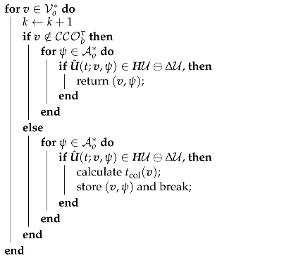return the pair $\left(\mathbf{v},\psi \right)$ that implies the largest $t_{\mathrm{col}}$

Algorithm 1 generates $n_v$ random velocity samples inside $\mathcal{V}\ominus \mathcal{B}\left({\mathbf{0}}_3,{ϵ}^v\right)$ and $n_{\psi }$ equally spaced samples inside $(-\pi ,\pi ]$, sorting them in ascending cost order. Then, it sequentially checks that each velocity sample does not result in a collision, i.e., if it does not belong to ${\mathcal{CCO}}_b^{\mathit{\tau }}$. When a velocity sample is collision-free, the algorithm tries to choose a heading sample that, given this collision-free velocity, respects the rotors’ thrust constraints. If such heading exists, the algorithm returns the corresponding pair of velocity and heading samples. On the other hand, when a velocity sample is not collision-free, the algorithm tries to choose a heading sample that respects the rotors’ thrust constraints and, if such heading exists, it calculates the time to collision for this particular pair of samples. Then, in the event that any velocity sample is free of collision, the algorithm returns the pair of samples that results in the minimum time to collision and respects the velocity and rotors’ thrust constraints. For this case, the main for loop in Algorithm 1 iterates $n_v$ times and, within each iteration, the nested else condition is executed. On the other hand, when the first velocity sample in ${\mathcal{V}}_o^{*}$ is collision-free and there is a heading sample that, given this first velocity sample, respects the rotors’ thrust constraints, the main for loop is executed only one time.

5. Numerical Simulation

The effectiveness of the proposed method is evaluated in a numerical simulation implemented on the basis of the nonlinear equations of motion (1) and (4)–(8) and coded in MATLAB utilizing the first-order explicit Euler method with a sampling time of 0.01 s. The vehicle adopted for the simulation is an x-shaped quadcopter with a mass of $1\mathrm{kg}$, arm length of 0.5 m, and inertia matrix ${\mathbf{J}}_b=\mathrm{diag}(0.015,0.015,0.03)$ kg m${}^2$.

The proposed method is compared with another one that uses the same control strategy and the original CCO [30] as the guidance strategy. To compare the methods, we conduct a Monte Carlo simulation where the quadcopter has an initial position $(0,0,5)$ m, zero initial velocity, and has to go to the desired position $(38,0,5)$ m, while avoiding collision with 270 quadcopters that are used to represent the obstacles, as depicted in Figure 5. The obstacles are arranged between the MAV’s initial and desired positions in thirty evenly spaced groups of nine. The kth group, where $k\in \{1,\dots ,30\}$, contains a static obstacle that has the randomly uniformly selected position offsets $\Delta y_{b,k}\in [-6,6]$ m and $\Delta z_{b,k}\in [-2,7]$ m relative to the line connecting the MAV’s initial and desired positions in the directions of ${\overrightarrow{y}}_r$ and ${\overrightarrow{z}}_r$, respectively. The remaining obstacles are circularly and uniformly distributed in the plane ${\overrightarrow{y}}_r$–${\overrightarrow{z}}_r$ and rotate around the static obstacle with a randomly uniformly selected radius ${\rho }_{b,k}\in [2,5]$ and angular velocity ${\overrightarrow{\mathit{\omega }}}_k\in \left([-0.4,-0.1]\cup [0.1,0.4]\right){\overrightarrow{x}}_r$.

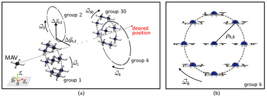
Figure 5. Schematic illustration of the proposed Monte Carlo simulation scenario. (a) Overview of the scenario showing the MAV, its target position, and the groups of obstacles. (b) The kth group of obstacles in detail, where $k\in \{1,\dots ,30\}$.

The vehicle can be circumscribed by a sphere of radius $0.5$ m, while all obstacles can be circumscribed by spheres of radius $0.7$ m. The controlled quadcopter has the following linear velocity and rotor thrust admissible sets:

$$\begin{array}{cc}\hfill \mathcal{V}& \triangleq \left\{\mathbf{v}\in {\mathbb{R}}^3|\parallel \mathbf{v}\parallel \le 5\right\},\hfill \\ \hfill \mathcal{F}& \triangleq \left\{{\mathbf{f}}^r\in {\mathbb{R}}^4|f_i\in \left[1.25,4\right],\forall i\in \{1,\dots ,4\}\right\}.\hfill \end{array}$$

Moreover, the vehicle is subject to the disturbances

$$\begin{array}{cc}\hfill {\mathbf{f}}_r^d\left(t\right)& =0.25{[1,-1,-1]}^{\mathrm{T}}\sin \left(0.5t\right)\mathrm{N},\hfill \\ \hfill {\mathit{\tau }}_b^d\left(t\right)& =0.005{[1,-1,-1]}^{\mathrm{T}}\sin \left(0.5t\right)\mathrm{Nm}.\hfill \end{array}$$

Table 1 shows the adopted parameters for the proposed guidance and control strategies.

Table 1. Parameters of the proposed method.

Control Law	Variable	Value
Attitude control law	${\mathbf{K}}_1$	diag(0.5, 0.5, 0.25)
	$\mathbf{C}$	$5{\mathbf{I}}_3$
	h	2
Position control law	${\mathbf{K}}_2$	$2.5{\mathbf{I}}_3$
	${\overline{\mathbf{K}}}_3$	$10{\mathbf{I}}_3$
	$t_s$	0.2 s
	${\mathbf{\Lambda }}_0^p$	$4{\mathbf{I}}_3$
	${\mathbf{\Lambda }}_1^p$	$2{\mathbf{I}}_3$
	${\mathbf{\Lambda }}_2^p$	${\mathbf{I}}_3$
	${\gamma }_p$	${\mathbf{I}}_3$
Guidance method	${\tau }_p$	$0.15$ s
	${ϵ}^r$	$0.06$ m
	${ϵ}^v$	$0.1$ m/s
	$\tau$	5 s
	n	2
	${\mathbf{\Lambda }}_0$	$4{\mathbf{I}}_3$
	${\mathbf{\Lambda }}_1$	$3{\mathbf{I}}_3$
	${\mathbf{\Lambda }}_2$	2${\mathbf{I}}_3$
	$\gamma$	$1.5{\mathbf{I}}_3$
	${\tau }_{\psi }$	$0.2$ s

Moreover, we have used in Algorithm 1 a total of 800 target velocity samples calculated using a uniform distribution over $\mathcal{V}\ominus \mathcal{B}\left({\mathbf{0}}_3,{ϵ}^v\right)$ and 50 equally spaced target heading samples inside the interval $(-\pi ,\pi ]$.

The MAV receives the desired heading signal (in degrees)

$$\check{\psi }\left(t\right)=\left\{\begin{array}{cc}0,\hfill & \mathrm{if}0\le t<2,\hfill \\ 50,\hfill & \mathrm{if}2\le t<5,\hfill \\ 10,\hfill & \mathrm{if}5\le t<8,\hfill \\ -30,\hfill & \mathrm{if}t\ge 8.\hfill \end{array}\right.$$

In order to conduct a more comprehensive analysis of the proposed method, we present in Figure 6 and Figure 7 the relevant results from a single iteration of the Monte Carlo simulation. A three-dimensional animation of this simulation is available at the following link: https://youtu.be/d7K4e6Ytn8M (accessed on 23 September 2023).

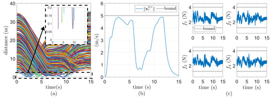
Figure 6. Constraint plots for the proposed method. (a) Distance from the quadcopter to the obstacles. (b) Euclidean norm of the quadcopter velocity and its bound. (c) Rotors’ thrusts and their bounds.

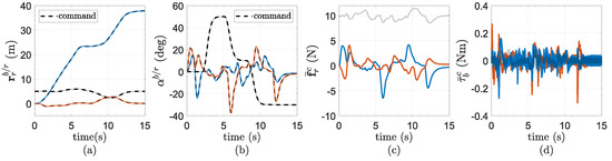
Figure 7. Position tracking performance, attitude tracking performance, and control commands for the proposed method. (a) Position tracking performance. (b) Attitude tracking performance. (c) Control force command. (d) Control torque command. Legend: ― vector first component, ― vector second component, and ― vector third component.

Figure 6a–c, respectively, show the distance between the quadcopter and the obstacles, the Euclidean norm of the quadcopter’s velocity and its bound, and the rotors’ thrust and their bounds. It can be seen that the proposed method guarantees the satisfaction of the position constraint (9), the linear velocity constraint (10), and the rotors’ thrust constraint (11), which demonstrates the effectiveness and robustness of the proposed method.

Figure 7 presents the position and attitude tracking performance as well as the force and torque control commands. In Figure 7a, it can be seen that the position commands are satisfactorily tracked despite the presence of the disturbance force. Figure 7b shows that the attitude commands are exactly tracked during the entire time despite the presence of the disturbance torque, thus confirming that by combining the proposed sliding mode attitude and smooth position control laws, an integral sliding mode exists in the attitude loop. This fact is also confirmed by Figure 8, which shows that the Euclidean norm of the attitude sliding variable $\mathbf{s}$ is restricted to a relatively small neighborhood of the origin during the entire time. Figure 7c and Figure 7d, respectively, show the force and torque control commands. These plots confirm the smoothness and the switching behavior of the force and torque control commands, respectively.

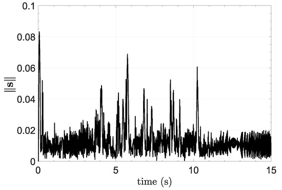
Figure 8. Euclidean norm of the attitude sliding variable $\mathbf{s}$.

5.1. Monte Carlo Simulation

We have performed, for each method, 100 iterations of the above-described Monte Carlo simulation. For both methods, we have analyzed at each iteration whether collisions have occurred and their number. For the proposed method, we have also analyzed whether the linear velocity and rotors’ thrust constraints are satisfied. Table 2 shows the Monte Carlo simulation results. It presents, for both methods, the collision rate ($CR$)

$$CR\triangleq \frac{n_c}{100},$$

where $n_c\in {\mathbb{Z}}_{\ge 0}$ is the number of iterations where collisions have occurred, and it also shows the average number of collisions per iteration ($ACI$)

$$ACI\triangleq \frac{n_{\mathrm{col}}}{100}CR,$$

where $n_{\mathrm{col}}\in {\mathbb{Z}}_{\ge 0}$ is the total number of collisions that have occurred in the 100 iterations. For the proposed method, Table 2 also shows the percentage of iterations in which the linear velocity and rotor thrust constraints are respected.

Table 2. Monte Carlo simulation results for the proposed and original CCO methods. N/A: not applicable.

	Proposed	Original CCO
$CR$	25%	50%
$ACI$	2.16	1.74
Respected velocity constraint	100%	N/A
Respected rotor thrust constraint	100%	N/A

The results in Table 2 confirm the effectiveness of the proposed method in respecting the linear velocity and rotors’ thrust constraints. Moreover, one can see that, by observing the obstacles’ acceleration and considering the vehicle position tracking error bound ${ϵ}^r$, the proposed method is more effective than the original CCO in preventing collisions. We emphasize that this is remarkable since the original CCO, by not considering the rotors’ thrust constraints, has more control force and torque available to avoid collisions. To support this statement, we also ran 100 iterations for the proposed method, disregarding the rotors’ thrust constraints. In this simulation, the proposed method had a $CR=0\%$, demonstrating that the previous $CR$ of 25% was only related to the inability to avoid collisions due to the control force and torque limitations imposed by the rotors’ thrust constraints.

5.2. Discussion

The results of the numerical simulations demonstrate the efficiency of the proposed method in guiding underactuated MAVs subject to model uncertainties/disturbances as well as velocity and rotors’ thrust constraints in the presence of obstacles that can accelerate. These results have practical importance given the recent growing interest in autonomous flight and the number of aircraft sharing the same air space. On the other hand, the performed simulation study, although comprehensive, did not consider sensor noise and inaccuracies. These uncertainties present in real-world scenarios could be immediately considered in the proposed strategy by suitably increasing the MAV tracking error bounds, the obstacles’ radii, and the guidance time horizon $\mathit{\tau }$. Moreover, it is worth mentioning that the proposed formulation considers that the MAV and the obstacles can be enclosed by spheres. While this is not a significant limitation, as more complex shapes can be approximated using a collection of spheres [43], there are situations where employing this approach might lead to an increased level of complexity to represent the obstacles.

6. Conclusions

This paper proposes robust guidance and control methods for underactuated MAVs equipped with fixed rotors subject to model uncertainties/disturbances and linear velocity and rotor thrust constraints, in the presence of accelerated obstacles. The attitude and position control laws are designed using a hierarchical SMC scheme that enforces the attitude-position TSS. The former is designed using a multi-input ISMC strategy and the latter is designed using a proportional–derivative policy combined with an SMDO. On the other hand, the proposed guidance strategy is based on the CCO and designed using a constraint-tightening approach for robustness against uncertainties/disturbances and a high-order SMD to robustly estimate the maximum accelerations of the obstacles. A Monte Carlo numerical simulation was performed using a quadcopter to compare the proposed method with another one that uses the same attitude and position control design and the original CCO in the guidance level. The proposed guidance method outperformed the original CCO in avoiding collisions with moving obstacles that can accelerate and, additionally, has been shown to be very effective in respecting linear velocity and rotor thrust constraints. In future works, the proposed method can be evaluated experimentally and applied to other mobile robotics systems. Moreover, Algorithm 1 can be further improved in performance, aiming at its implementation in embedded systems.

References

- Singireddy, S.R.R.; Daim, T.U. Technology Roadmap: Drone Delivery—Amazon Prime Air. In Infrastructure and Technology Management: Contributions from the Energy, Healthcare and Transportation Sectors; Springer International Publishing: Cham, Switzerland, 2018; pp. 387–412. [Google Scholar]
- Rajendran, S.; Srinivas, S. Air taxi service for urban mobility: A critical review of recent developments, future challenges, and opportunities. Transp. Res. Part Logist. Transp. Rev. 2020, 143, 102090. [Google Scholar] [CrossRef]
- Santos, D.A.; Lagoa, C.M. Wayset-based guidance of multirotor aerial vehicles using robust tube-based model predictive control. ISA Trans. 2022, 128, 123–135. [Google Scholar] [CrossRef] [PubMed]
- Utkin, V.I. Sliding Modes in Control and Optimization; Springer: Berlin/Heidelberg, Germany, 1992. [Google Scholar]
- Drajunov, S.V.; Utkin, V.I. Sliding mode control in dynamic systems. Int. J. Control 1991, 55, 1029–1037. [Google Scholar] [CrossRef]
- Besnard, L.; Shtessel, Y.B.; Landrum, B. Quadrotor vehicle control via sliding mode controller driven by sliding mode disturbance observer. J. Frankl. Inst. 2012, 349, 658–684. [Google Scholar] [CrossRef]
- Muñoz Palacios, F.; Espinoza Quesada, E.S.; González, I.; Salazar, S.; Lozano, R. Robust Trajectory Tracking for Unmanned Aircraft Systems using a Nonsingular Terminal Modified Super-Twisting Sliding Mode Controller. J. Intell. Robot. Syst. 2019, 93, 55–72. [Google Scholar] [CrossRef]
- Silva, A.L.; Santos, D.A. Fast Nonsingular Terminal Sliding Mode Flight Control for Multirotor Aerial Vehicles. IEEE Trans. Aerosp. Electron. Syst. 2020, 56, 4288–4299. [Google Scholar] [CrossRef]
- Labbadi, M.; Cherkaoui, M. Robust adaptive nonsingular fast terminal sliding-mode tracking control for an uncertain quadrotor UAV subjected to disturbances. ISA Trans. 2020, 99, 290–304. [Google Scholar] [CrossRef]
- Wang, X.; Sun, S.; van Kampen, E.J.; Chu, Q. Quadrotor Fault Tolerant Incremental Sliding Mode Control driven by Sliding Mode Disturbance Observers. Aerosp. Sci. Technol. 2019, 87, 417–430. [Google Scholar] [CrossRef]
- Ricardo, J.A., Jr.; Santos, D.A. Smooth second-order sliding mode control for fully actuated multirotor aerial vehicles. ISA Trans. 2022, 129, 169–178. [Google Scholar] [CrossRef]
- Slotine, J.J.E. The Robust Control of Robot Manipulators. Int. J. Robot. Res. 1985, 4, 49–64. [Google Scholar] [CrossRef]
- Lu, Y.S.; Chen, J.S. Design of a global sliding-mode controller for a motor drive with bounded control. Int. J. Control 1995, 62, 1001–1019. [Google Scholar] [CrossRef]
- Utkin, V.; Shi, J. Integral sliding mode in systems operating under uncertainty conditions. In Proceedings of the 35th IEEE Conference on Decision and Control, Kobe, Japan, 11–13 December 1996; Volume 4, pp. 4591–4596. [Google Scholar]
- Bartoszewicz, A. Time-varying sliding modes for second-order systems. IEE Proc.—Control Theory Appl. 1996, 143, 455–462. [Google Scholar] [CrossRef]
- Ricardo, J.A., Jr.; Santos, D.A. Robot Guidance and Control Using Global Sliding Modes and Acceleration Velocity Obstacles. In Proceedings of the International Workshop on Variable Structure Systems and Sliding Mode Control, Rio de Janeiro, Brazil, 11–14 September 2022. [Google Scholar]
- Altug, E.; Ostrowski, J.; Mahony, R. Control of a quadrotor helicopter using visual feedback. In Proceedings of the 2002 IEEE International Conference on Robotics and Automation (Cat. No.02CH37292), Washington, DC, USA, 11–15 May 2002; Volume 1, pp. 72–77. [Google Scholar]
- Bertrand, S.; Guénard, N.; Hamel, T.; Piet-Lahanier, H.; Eck, L. A hierarchical controller for miniature VTOL UAVs: Design and stability analysis using singular perturbation theory. Control Eng. Pract. 2011, 19, 1099–1108. [Google Scholar] [CrossRef]
- Liu, H.; Bai, Y.; Lu, G.; Shi, Z.; Zhong, Y. Robust tracking control of a quadrotor helicopter. J. Intell. Robot. Syst. 2014, 75, 595–608. [Google Scholar] [CrossRef]
- Antonelli, G.; Cataldi, E.; Arrichiello, F.; Robuffo Giordano, P.; Chiaverini, S.; Franchi, A. Adaptive Trajectory Tracking for Quadrotor MAVs in Presence of Parameter Uncertainties and External Disturbances. IEEE Trans. Control. Syst. Technol. 2018, 26, 248–254. [Google Scholar] [CrossRef]
- Hou, Z.; Yu, X.; Lu, P. Terminal Sliding Mode Control for Quadrotors with Chattering Reduction and Disturbances Estimator: Theory and Application. J. Intell. Robot. Syst. 2022, 105, 1–21. [Google Scholar] [CrossRef]
- Fridman, L. Recent Achievement and Perspective Directions in Sliding Mode Control. In Proceedings of the 22st IFAC World Congress, Yokohama, Japan, 9–14 July 2023; pp. 1–5. [Google Scholar]
- Kamel, M.; Alonso-Mora, J.; Siegwart, R.; Nieto, J. Robust collision avoidance for multiple micro aerial vehicles using nonlinear model predictive control. In Proceedings of the 2017 IEEE/RSJ International Conference on Intelligent Robots and Systems (IROS), Vancouver, BC, Canada, 24–28 September 2017; pp. 236–243. [Google Scholar]
- Pereira, J.C.; Leite, V.J.S.; Raffo, G.V. An ellipsoidal-polytopic based approach for aggressive navigation using nonlinear model predictive control. In Proceedings of the 2021 International Conference on Unmanned Aircraft Systems (ICUAS), Athens, Greece, 15–18 June 2021; pp. 827–835. [Google Scholar]
- Bouzid, Y.; Bestaoui, Y.; Siguerdidjane, H. Quadrotor-UAV optimal coverage path planning in cluttered environment with a limited onboard energy. In Proceedings of the 2017 IEEE/RSJ International Conference on Intelligent Robots and Systems (IROS), Vancouver, BC, Canada, 24–28 September 2017; pp. 979–984. [Google Scholar]
- Fiorini, P.; Shiller, Z. Motion planning in dynamic environments using velocity obstacles. Int. J. Robot. Res. 1998, 17, 760–772. [Google Scholar] [CrossRef]
- Bareiss, D.; Van Den Berg, J. Reciprocal collision avoidance for robots with linear dynamics using LQR-Obstacles. In Proceedings of the 2013 IEEE International Conference on Robotics and Automation, Karlsruhe, German, 6–10 May 2013; pp. 3847–3853. [Google Scholar]
- Ricardo, J.A., Jr.; Santos, D.A. Robust Collision Avoidance for Mobile Robots in the Presence of Moving Obstacles. IEEE Control Syst. Lett. 2023, 7, 1584–1589. [Google Scholar] [CrossRef]
- Van Den Berg, J.; Snape, J.; Guy, S.J.; Manocha, D. Reciprocal collision avoidance with acceleration-velocity obstacles. In Proceedings of the IEEE International Conference on Robotics and Automation, Shanghai, China, 9–13 May 2011; pp. 3475–3482. [Google Scholar]
- Rufli, M.; Alonso-Mora, J.; Siegwart, R. Reciprocal Collision Avoidance With Motion Continuity Constraints. IEEE Trans. Robot. 2013, 29, 899–912. [Google Scholar] [CrossRef]
- Levant, A. Higher-order sliding modes, differentiation and output-feedback control. Int. J. Control 2003, 76, 924–941. [Google Scholar] [CrossRef]
- Levant, A. Sliding order and sliding accuracy in sliding mode control. Int. J. Control 1993, 58, 1247–1263. [Google Scholar] [CrossRef]
- Markley, F.L.; Crassidis, J.L. Fundamentals of Spacecraft Attitude Determination and Control; Space Technology Library; Springer: New York, NY, USA, 2014. [Google Scholar]
- Goldstein, H. Classical Mechanics; Addison-Wesley: Boston, MA, USA, 1980. [Google Scholar]
- Bezerra, J.A.; Santos, D.A. Optimal Exact Control Allocation for Under-Actuated Multirotor Aerial Vehicles. IEEE Control Syst. Lett. 2022, 6, 1448–1453. [Google Scholar] [CrossRef]
- Sakurama, K.; Verriest, E.I.; Egerstedt, M. Effects of insufficient time-scale separation in cascaded, networked systems. In Proceedings of the 2015 American Control Conference (ACC), Chicago, IL, USA, 1–3 July 2015; pp. 4683–4688. [Google Scholar]
- Bhat, S.P.; Bernstein, D.S. Finite-Time Stability of Continuous Autonomous Systems. SIAM J. Control. Optim. 2000, 38, 751–766. [Google Scholar] [CrossRef]
- Ricardo, J.A., Jr.; Santos, D.A. Attitude Tracking Control for a Quadrotor Aerial Robot Using Adaptive Sliding Modes. In Proceedings of the XLI Ibero-Latin-American Congress on Computational Methods in Engineering, Foz do Iguaçu, Brazil, 16–19 November 2020. [Google Scholar]
- Escareño, J.; Salazar, S.; Romero, H.; Lozano, R. Trajectory control of a quadrotor subject to 2D wind disturbances. J. Intell. Robot. Syst. 2013, 70, 51–63. [Google Scholar] [CrossRef]
- Ducard, G.; Hua, M.D. Discussion and practical aspects on control allocation for a multi-rotor helicopter. Int. Arch. Photogramm. Remote. Sens. Spat. Inf. Sci. 2011, 38, 95–100. [Google Scholar] [CrossRef]
- Sinha, A.; Malo, P.; Deb, K. A Review on Bilevel Optimization: From Classical to Evolutionary Approaches and Applications. IEEE Trans. Evol. Comput. 2018, 22, 276–295. [Google Scholar] [CrossRef]
- Van Den Berg, J.; Lin, M.; Manocha, D. Reciprocal Velocity Obstacles for Real-Time Multi-Agent Navigation. IEEE Trans. Robot. 2007, 23, 834. [Google Scholar] [CrossRef]
- O’Rourke, J.; Badler, N. Decomposition of three-dimensional objects into spheres. IEEE Trans. Pattern Anal. Mach. Intell. 1979, 3, 295–305. [Google Scholar] [CrossRef]
Disclaimer/Publisher’s Note: The statements, opinions and data contained in all publications are solely those of the individual author(s) and contributor(s) and not of MDPI and/or the editor(s). MDPI and/or the editor(s) disclaim responsibility for any injury to people or property resulting from any ideas, methods, instructions or products referred to in the content. |
© 2023 by the authors. Licensee MDPI, Basel, Switzerland. This article is an open access article distributed under the terms and conditions of the Creative Commons Attribution (CC BY) license (https://creativecommons.org/licenses/by/4.0/).