Abstract
UAV formation keeping is an important research element due to its cooperative formation control. This study proposes a passive positioning model for UAVs based on the Monte Carlo strategy and provides a trajectory programming decision scheme based on the predicted calculation of deviated UAV predefined endpoint locations, effectively improving the efficiency of UAVs performing formation-keeping tasks during flight. Then, the simulation after sampling by Gaussian distribution is used to obtain the trajectory planning under simultaneous control of multiple cluster formations, and the feasibility, accuracy and stability of the proposed model are verified. This study provides useful guidance for UAV formation control applications.
1. Introduction
In recent years, UAVs have been used in a wide range of military and civilian applications, such as for air transport [1], communication in areas affected by natural disasters [2], search and rescue [3], and magnetic measurements [4]. UAV formation flying is an organizational model in which multiple UAVs are arranged in a certain formation and assigned according to the mission requirements when performing search and rescue, surveillance or coverage control missions [3,5]. Its central concern is to keep the prescribed formation and fully utilize the aircraft’s performance [6]. This requires positioning adjustments for the UAV in flight. The passive location uses the UAV’s signals for location rather than the UAV actively transmitting signals, which reduces the requirements for equipment and scenarios [7]. The more stations there are located in the area, the higher their positioning accuracy and the more flexible they are in applications [8]. Passive location technology has gradually become a trend in the field of air shows or electronic countermeasures.
UAV formation keeping is an integral part of UAV formation flight, and its essence is an optimization problem. When designing a formation keeping adjustment scheme for a UAV, its formation flight pattern is first determined. Then, an optimal UAV scheduling solution for returning UAVs to standard formation positions for formation flight is created based on the deviation of relative location and relative angle. UAV clusters can achieve effective and accurate location of UAVs by using four-station passive location [9]. The other signals except for the signals emitted by these four UAVs are all electromagnetic interference. The current electromagnetic environment is becoming increasingly complex. To avoid interference from external signals, UAVs should maintain electromagnetic silence as much as possible and emit fewer electromagnetic wave signals to the outside [10].
Yao et al. [11] proposed an algorithm based on perturbed fluid and trajectory propagation to solve the three-dimensional path planning problem of UAVs in static environments. A.C. and D.D. [12] proposed a three-dimensional path planning scheme for UAVs based on the Reverse Firefly Swarm Optimization (RGSO) algorithm, based on which the trajectories were further optimized and smoothed to determine the trajectory planning of UAVs. All of these studies are good at providing a method for UAV trajectory planning or waypoint assignment, which improves the efficiency of UAVs to perform certain tasks. However, there remain very few research results on these topics in order to enable the precise control of the formation time during a quadrotor UAV cluster mission execution, so that the quadrotor UAV cluster can form the desired formation shape efficiently within a predetermined time, or precisely control the beginning and end positions of the UAVs during flight for a period of time to achieve the effect of that the UAVs maintaining a certain formation shape and not deviating from it. Wu et al. [13] studied the use of genetic algorithms mixed with simulated annealing algorithms for the beginning and end locations of UAVs and the planning of the trajectory decision scheme during UAV formation transformation, effectively reducing the UAV computation time. However, they did not consider the study and path planning of the beginning and end locations of the trajectory when the deviating UAV maintains its formation. Li et al. [14] introduced the concept of “predefined time” in their study of UAV formation control and determined a method for calculating stable and accurate predicted time bounds for UAV trajectory planning during formation-keeping missions. However, they did not consider the effect of the initial location where the UAV deviation occurred versus the predicted focus location of the UAV target obtained on the trajectory planning. Inspired by the above discussion, this study focuses on the optimization of the target focus location in the formation keeping trajectory during UAV flight and the corresponding trajectory planning within a certain time frame.
First, to keep the UAV as electromagnetically silent as possible, we established an innovative control method for the transformed leader-follower method with the smallest total electromagnetic wave signal emitted by the UAV as the objective function. Then, we used the circular formation flight pattern as the fundamental research object, and the error in follower UAVs’ coordinates as the objective function and built the optimization model to make the UAV location error as small as possible and obtained the precise location for the follower adjustment. Then, this study determines the location adjustment trajectory to be maintained by the UAV formation by considering how to make the change in speed and force smooth when the UAV location changes. To verify the accuracy and stability of the model, we sampled the ideal location coordinates of the follower with Gaussian distribution [15], substituted the initial coordinate data of the random UAV to be adjusted into the model for analysis and verification, and obtained the precise location of the follower adjustment and the control method of the transformed leader-follower method. Finally, this study is extended based on circular formation flight patterns and discusses passive location models for different shape formation flight patterns. The architecture of the paper is organized as follows. Section 2 presents three models: a model for continuous UAV assignment under complex constraints based on the transformed leader-follower method; a model for UAV location adjustment to determine the target location under UAV formation keeping; and a model for trajectory planning to enable UAV formation keeping. Section 3 integrates a set of data from the dataset obtained from Gaussian distribution sampling into the above model for simulation to verify the accuracy of the model. Section 4 obtains the simulation results of the empirical analysis and performs a sensitivity analysis of the weights of distance deviation and angle deviation to determine the accuracy of the model. Section 5 discusses the impact of algorithm computational complexity and battery consumption on the efficiency of UAVs performing formation-keeping tasks. This study provides a decision scheme that enables more accurate target waypoint locations for track planning for UAV cluster formation maintenance and makes UAV adjustment more efficient.
2. Establishment of the Model: Take Circular Formation Flight as an Example
Since other flight formation patterns with different numbers of UAVs can be converted into a combination of several circles, for the convenience of the modeling and analyzing, we assume that m UAVs are flying in a circular formation at the same altitude. Among these m UAVs, one UAV (FY00) is located in the center of the circular formation, and the remaining UAVs (FY01-FY0m-1) are evenly distributed on a certain circumference. The radius of the circumference is R. The UAV adjusts its location using a purely azimuthal passive location method. This method involves a few UAVs in the formation transmitting signals and the rest passively receiving them, and the received direction information is the angle between the lines of a UAV receiving the signal and the UAVs transmitting the signals. To maintain the formation of the UAV clusters in flight, the following model was developed in this study.
2.1. Assumptions of the Model
Assumption 1.
Assuming that the UAVs all remain at the same altitude.
Assumption 2.
Assuming that the UAV clusters make a uniform flight with speed v.
Assumption 3.
Assuming that the locations of UAV FY00 and FY01 are always in standard position coordinates.
2.2. The Establishment of the Transformed Leader-Follower Model
This model considers a reasonable UAV location adjustment scheme so that the m − 1 UAVs except for FY00 are finally evenly distributed on the circumference. The two elements of whether the UAV transmits or receives signals, and the position deviation are considered together, i.e., the distance between every two UAVs is simply considered as a weight, and the UAV location adjustment scheme is determined under reasonable constraints based on the assignment problem in 0–1 programming [16]. Assuming that the position of the i UAV at the nth moment is expressed in polar coordinates as , the coordinates of the i UAV at the next moment (after adjustment) are expressed as , where . The two position coordinates are obtained from the polar coordinate system established at different moments with the UAV FY00 position coordinates as the center of the circle, and the line connecting UAV FY00 and FY01 as the horizontal axis.
The model introduces two factors to determine whether the UAV is the leader (UAVs that transmit signals) or follower (UAVs that receive signals) when in formation: one is the deviation tendency factor and the other is the distance tendency factor , where . is the degree of deviation of the UAV from its standard location and reflects the priority of the UAV to receive dispatch. is the weight of the distance length of the two UAVs on the circumference, reflecting the trade-off between the leader UAVs in the special case where the two transmitting signal UAVs have a small difference in deviation tendency factor but a large difference in distance from the adjusted UAV. This model considers preferentially using the UAV with a smaller deviation tendency factor and distance tendency factor to adjust the other UAVs.
- Determination of deviation tendency factor
Since the UAV FY01 is already in a standard position, we do not consider it to receive signals. Let a random variable be:
where .
The initial location of each UAV has some deviation from its standard location. This model prioritizes the adjustment of UAVs with larger location deviations using UAVs with smaller location deviations. The deviation tendency factor depends on the distance deviation and angle deviation of this UAV. The former is the distance of the point from the center of the circle. The latter is the angle between the line of the point and the center of the circle and the horizontal direction.
Let the weights of distance deviation and angle deviation be and , respectively. is the sum of distance deviation and angle deviation of m − 1 UAVs. According to the different weights of distance deviation and angle deviation, the following equation can be obtained.
The standard deviation method is usually used in determining the weights of two indicators. The greater the standard deviation of an indicator, the greater the variability of the indicator value, the greater the amount of information provided, the greater the role in the comprehensive evaluation, and the greater the weight of the indicator [17].
Because of the difference in the magnitude of the distance and angle, to eliminate the influence of the magnitude, the data need to be standardized [18]. In normalization, for the convenience of calculation, we define the arc length of the ith UAV as the length of the arc formed by the ith UAV and its neighboring previous UAV, and use this to replace the calculation of the angle weight. The arc length formula can be used to convert the angle of the central angle of the circle into the corresponding arc length, thus the two sets of data have the same magnitude. In this case, the standard value of the distance between the UAV and the center of the circle is , and the standard value of the arc length is . After eliminating the effect of dimensionality, the standard deviations of the standardized distance (polar diameter) and angle (polar angle) are calculated separately to determine the weights of the two indicators.
Generally, for the purpose of data processing, the data are usually mapped to the range of 0 to 1, which is the normalization of the data. This makes the processing easier and faster. Therefore, the largest value of corresponding to the m − 1 UAVs obtained, needs to be recorded as 1, and the rest are scaled down equally so that all lie in the range of zero to one.
- Determination of distance tendency factor
When the deviation tendency factors of two UAVs are similar, the UAV that is relatively close to the UAV being adjusted is considered for adjustment—that is, to minimize the distance tendency factor of the UAV.
In order to make the adjustment scheme more reasonable, we need to keep the number of wires between the transmitting signal and the receiving UAV as small as possible. That is, the UAV should maintain electromagnetic silence as much as possible, with fewer electromagnetic wave signals to avoid interference from outside signals. This model considers the deviation propensity factor and the distance propensity factor, and defines the product of the two with as the amount of information, from which the objective function can be obtained as follows.
This model considers the need to keep the UAVs as electromagnetically silent as possible so that up to three UAVs on the circumference transmit signals in a single attempt. The effective location of the UAV cannot be obtained when there is only one UAV transmitting signals on the circumference, so we consider two or three UAVs transmitting signals on the circumference. Theoretically, with a greater the degree of deviation, the UAV needs to be adjusted by the increased number of UAVs. This model prioritizes the adjustment of UAVs with a greater degree of deviation from the standard location. The distance factor of the two factors in position deviation is given priority, and angle deviation is considered when the distance deviation is the same.
Based on the above objectives and constraints, the 0–1 programming model is developed as follows.
2.3. The Establishment of the UAV Location Adjustment Model
When the adjusted UAV’s location is closer to its standard location, the adjustment scheme is more reasonable. The objective function can be obtained as follows.
The constraint is that the distance deviation and angle deviation of the UAV after adjustment are less than its deviation before adjustment. According to the Gaussian distribution Law, there will be a small number of UAVs with large initial distance deviation or large initial angle deviation. Therefore, it is necessary to introduce the correction coefficient for distance deviation or angle deviation with large deviation to reduce the impact of excessive deviation on the results.
Based on the above objectives and constraints, the model is developed as follows.
2.4. The UAV Location Adjustment Trajectory Planning Model
2.4.1. Minimum-Jerk Trajectory Planning
The displacement function of the UAV for location adjustment can be expressed in vector form as .
Let there be a total of waypoints including the adjustment start and end points when the UAV is making location adjustments. At the moment , each UAV needs to reach the corresponding position coordinates obtained from the UAV location adjustment model in Section 2.3 of this study. We define it as the kth waypoint . represents the starting point of the location adjustment performed by the UAV, and represents the end point of the location adjustment performed by the UAV. We record the waypoints as:
Thus, we divide the trajectory of the UAV location adjustment, i.e., the route to be planned, into segments.
In this study, the minimum-jerk trajectory planning proposed by Vijay Kumar is used to find the optimal path for UAV location adjustment [19,20]. Jitter in the desired UAV trajectory can adversely affect the performance of the manipulator’s tracking control algorithm [21]. To reduce this effect, it is important to make the change in UAV output force as smooth as possible, i.e., to make the change in UAV acceleration as smooth as possible, so that the jerk of the UAV is minimized.
Obtaining minimum jerk involves making the action S of the following equation obtain a minimal value.
Extending the Euler-Lagrange equation, the following equation can be obtained.
Substituting into the above equation, the path to obtain the jerk minimization needs to satisfy:
The above equation shows that the displacement functions and between every two adjacent waypoints can be described by a fifth-order polynomial.
The motion of the UAV in x dimensions, between the kth waypoint and the (k+1)th waypoint, has the following relation.
There are segments of the route to be planned, and each segment will have six pending coefficients, so this route planning will have parameters to be solved for.
2.4.2. Solving for Parameters
- At the beginning and end of each segment, each UAV needs to reach the identified coordinates of the corresponding position, i.e., the corresponding polynomial function must give coordinates that coincide with the waypoint.
The above equation expands a total of equations.
- When the UAV performs location adjustment, the initial and final velocity of the flight are both v, and the initial and final acceleration are both zero.
The above equation expands a total of 4 equations.
- The articulation of the kth segment and the (k+1)th segment should be silky smooth, and there should be no abrupt changes in velocity and acceleration.
The above equation expands a total of equations.
- To ensure further that the moment output can vary smoothly, the continuity of the third- and fourth-order derivatives on the segment boundary needs to be constrained.
The above equation expands a total of equations.
From the above analysis, we can establish a total of equations, from which we can solve the values of each parameter and determine the motion trajectory of the UAV in x dimensions. The motion planning of each dimension in UAV flight can be seen being as independent of each other. Therefore, the motion planning for the remaining dimensions can be derived in the same way.
3. Empirical Analysis
3.1. UAV Location Adjustment
This study assumes that 10 UAVs fly in a circular formation, with one UAV (FY00) at the center of the circle and the remaining nine UAVs (FY01-FY09) evenly distributed around the circumference of the circle with a radius of 100 m. The coordinates of the UAV location equal a data set with an infinite number of samples, which prevents a complete coverage analysis. From the central limit theorem, it follows that the probability distributions of many random variables obey or approximately obey a Gaussian distribution. Therefore, this study achieves fast model validation by Gaussian distribution Sampling. In this paper, data sets are sampled by Gaussian distribution, and one set of data (Table A1 in Appendix A) are taken for example analysis, and the rest of the data are analyzed in the same way. The analysis is as follows.
- (a)
- Data Standardization
The distance and acr-length-related data was standardized as shown in Table 1.

Table 1.
Standardized distance- and arc-length-related data.
- (b)
- Calculation of the standard deviation of the distance (polar diameter) and angle (polar angle) :
- (c)
- Obtaining the distance and angle weights , :
Based on the initial UAV location, it can be seen that the angle deviation is very small and brings minimal impact. The results calculated based on , also confirm the accuracy of the model in calculating the weights using the standard deviation method.
We calculate and normalize it to obtain the following Table 2.
Table 2.
The value of the normalized deviation tendency factor .
Analyzing the initial position coordinates of each UAV, the three UAVs numbered FY03, FY06, and FY09 deviated to a greater extent and were adjusted using three UAVs, while the rest of the UAVs were adjusted using two UAVs.
The transformed leader-follower model is as follows.
From the above model, the UAVs transmitting and receiving signals can be identified, and the preliminary results were shown in Section 4.1.
Due to the large weight of the distance deviation in the initial position coordinates of this group of UAVs, its influence on the results is greater; therefore, we consider introducing a correction coefficient for the distance deviation and make the angle deviation correction coefficient . The UAV location adjustment model is as follows.
The specific schemes for UAVs adjustment obtained without () and with () the introduction of the distance deviation correction coefficient are shown in Section 4.2, respectively.
3.2. UAV Trajectory Planning
The speed of the UAV cluster in uniform flight is: [22]. We obtained from the simulation that the UAV that deviated from the standard location converged to the standard location after one adjustment. After the two adjustments, the location has completely converged to the standard location. Here, we divide the trajectory of UAV location adjustment into two segments, i.e., . From Equation (12) to Equation (15), the following equations are obtained.
The above system of equations containing 12 equations is expressed in matrix form, and the values of the 12 parameters can be obtained by finding the inverse of the coefficient matrix to obtain the UAV’s trajectory planning equations in x dimensions.
The trajectory planning equations for the nine UAVs are shown in Section 4.3.
4. Results
4.1. Preliminary Scheme of UAV Adjustment Based on the Transformed Leader-Follower Model
The preliminary adjustment scheme for determining the transmitting and receiving signal UAVs is shown below.
In the above figure, the starting segment of the arrow is the UAV transmitting the signal, and the terminating end of the arrow is the UAV receiving the signal.
From Figure 1, the UAV with a smaller deviation tendency factor transmits more signals, while the UAV that receives signals has a larger deviation tendency factor. In the above figure, UAV FY05 received the signals emitted by UAVs FY06 and FY07. Among them, the deviation tendency factor of UAV FY06 is significantly larger, and the reason for choosing this UAV is the smaller distance tendency factor between UAVs FY05 and FY06. Therefore, this model should consider both the deviation tendency factor and the distance tendency factor when adjusting the UAV location. The model is reasonably established.
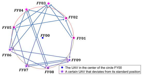
Figure 1.
Preliminary adjustment scheme figure for UAVs.
4.2. Specific Scheme of UAV Location Adjustment
The deviation tendency factor determines the adjustment order of the UAV. The larger the of the UAV, the earlier the adjustment of it. Therefore, the specific order in which the UAVs were adjusted was: FY09 was adjusted by FY01, FY07, and FY08; FY03 was adjusted by FY01, FY02, and FY05; FY06 was adjusted by FY03, FY04, and FY09; FY04 was adjusted by FY02 and FY08; FY07 was adjusted by FY03 and FY09; FY08 was adjusted by FY04 and FY06; FY05 was adjusted by FY06 and FY07; and FY02 was adjusted by FY01 and FY05.
From Table 3, if the correction coefficient is not introduced, it can be seen that the UAV locations have been significantly improved when the objective function is smallest, but there are still individual UAVs with a large degree of deviation from the standard location. This is due to the minimization of the objective function with the sacrifice of a certain UAV—that is, ignoring the adjustment of the deviation location of the UAV. To avoid this case, this model introduced a correction coefficient of . Due to the large weight of the distance deviation and its influence on the results, only the distance deviation was corrected.
Table 3.
Specific scheme table of UAV location adjustment.
We calculate the standard deviation of distance and angle deviation quantities before and after the introduction of correction coefficient.
From Equation (24), The standard deviation of the two deviation quantities was significantly reduced after the introduction of the correction coefficient, and the UAV was adjusted to be close to its standard location whether the correction coefficient was introduced or not. This verified that it is reasonable to introduce the correction coefficient. Since the UAVs cannot maintain a strict relative standstill in formation flight, the coordinates obtained from the adjustment will be somewhat different from the standard coordinates, but the model is reasonable within the error allowance.
The specific scheme of the UAV adjustment before and after the introduction of the correction coefficient was plotted as follows.
From Figure 2, the UAV location with the correction coefficient represented by the red pentagram is closer to the standard location than the UAV location without the correction coefficient represented by the blue pentagram, and both obtain better results than the initial location.
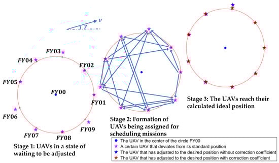
Figure 2.
Specific adjustment scheme figure for UAVs.
4.3. Results of UAV Trajectory Planning
Table 4 shows the trajectory equation for UAV location adjustment, based on which, we obtain the results of UAV trajectory planning as shown in Figure 3. From Figure 3, when the location adjustment of the UAV’s trajectory is one segment, the UAV cluster moves at the moment to the coordinate position at the moment calculated by the above model according to the black curve’s trajectory. The accuracy of the above model can be verified. When the UAV’s location adjustment trajectory is divided into two segments, the connection between the first segment of the trajectory, indicated by the green line, and the second segment of the trajectory, indicated by the light blue line, is smooth. That is, there is no abrupt change in speed and acceleration as the UAV moves from the first trajectory to the second trajectory. Jerk means a change in force, and a drastic change in power can make the UAV less controllable. Therefore, the UAV should ensure that the change in force during the location adjustment flight is as smooth as possible, i.e., the change in acceleration is smooth. Although the trajectory is not the shortest trajectory connecting waypoints, such a trajectory ensures the smooth flight of the UAV. Since the dimensions between trajectories are independent of each other, the model of this study can also be extended to three-dimensional UAV location adjustment simulation.
Table 4.
Trajectory equation for UAV location adjustment.
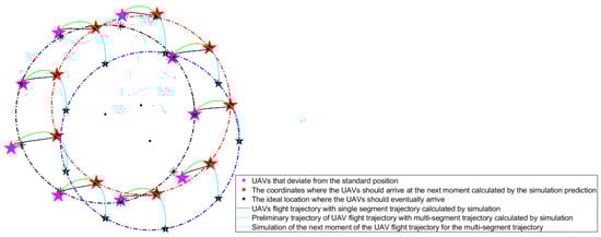
Figure 3.
Track figure of UAV location adjustment.
Since the dimensions between trajectories are independent of each other, the model of this study can also be extended to three-dimensional UAV location adjustment simulation.
From Figure 4, the adjusted position coordinates of all UAVs selected by Gaussian distribution sampling are closer to the standard position coordinates than the initial position coordinates. The trajectories of the UAV clusters in the sample set all converge to the ideal coordinate points. The model developed in this paper is reasonable and accurate.
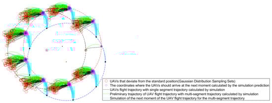
Figure 4.
Trajectory simulation of UAV cluster formation keeping with Gaussian distribution sampling.
4.4. Sensitivity Analysis of the Simulation Results of UAV Adjustment on the Weights
In the adjustment scheme for the UAV, we applied the standard deviation method to determine the weights of the distance deviation and the angle deviation quantity. To verify the stability of the model, we change the distance deviation weight and angle deviation weight to analyze the sensitivity of the weights in the above data to the polar coordinate values of the UAV’s adjusted location.
From Figure 5a, when the distance deviation weight is larger, the distance deviation quantity obtained is smaller (the image reflects that the amplitude of the distance away from the standard value becomes smaller and smaller as increases), and the distance (polar diameter) is closer to the standard value. From Figure 5b, the larger the angle deviation weight (), the closer the line representing the angle (polar angle) is to the standard value, represented by the red line. That is, the larger the angle deviation weight, the more the polar angle deviates from the standard value.
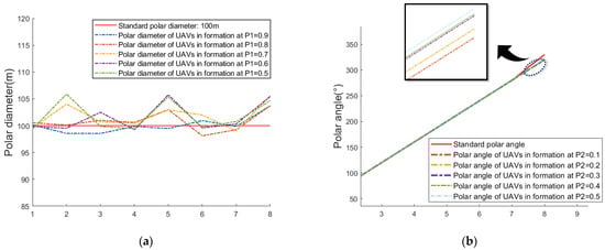
Figure 5.
Polar diameter and polar angle values with different distance and angle deviation weights. (a) Polar diameter values with different distance deviation weights. (b) Polar angle values with different angle deviation weights.
The relationship between distance and angle deviation quantity and weight () is as follows.
5. Discussion
When the formation of UAVs is more complex (the formation is a shape containing curves or the number of UAVs is large, etc.), the graph of the formation can also be converted into a combination of several circles, and then the actual position coordinates of the UAVs can be determined and adjusted according to the model of this study. Using a conical formation of several UAVs as an example (Figure A1 in Appendix B), the process of adjusting the location of the UAVs is as follows: a certain UAV is first identified as the origin of the polar coordinate system, and the cone is converted into a number of circular combinations. The UAV on any of the circumferences can determine its actual initial position coordinates by the received azimuth information, and then the specific adjustment scheme of the UAV is determined by the above model.
In this study, the relationship between the two weights and the model has been analyzed and a set of data obtained by sampling have been calculated to reflect that different parameter selections may lead to different adjustment results. Figure 6 reflects the relationship between the quantity of distance deviation and the quantity of angle deviation we obtained for the adjusted position in the polar coordinate system as the weight of distance deviation and the weight of angle deviation are changed. It can be seen that as increases, the deviation quantity from the distance of the calculated adjustment position becomes smaller and smaller, and conversely as decreases, at the same time the deviation quantity from the angle of the calculated adjustment position becomes larger and larger. However, when exceeds a certain value, the objective accuracy of the adjusted position decreases instead. It is calculated that when is greater than 0.976, the above rule is not fully obeyed, which means that the angle offset will become larger and larger when is too small. That means we have to consider both weights in an integrated way, and the change in the weights affects the degree of distance and angle correction, so the weights should be studied more deeply when developing the adjustment scheme for the UAV.
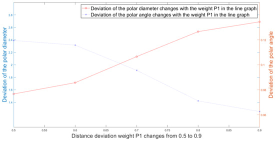
Figure 6.
The relationship between distance and angle deviation quantity and weight ().
The effect of other parameters mentioned in the model on the results can also be further analyzed—for example, the bias correction coefficient introduced in the model in this study. Since the deviations of the UAV deviations obey the Gaussian distribution law, there will be a small number of UAVs with large initial position deviations or large initial angle deviations, resulting in a certain weight being too large and having a huge impact on the results. Therefore, the introduction of deviation coefficients makes the calculation results converge faster, the search range that meets the constraints becomes smaller, and the adjusted coordinates become closer to the standard coordinates. To adjust the UAV position coordinates more accurately, the value of the correction coefficient needs to be reduced, but also the adjustment speed of the UAVs needs to be slowed down. Therefore, through the above analysis, this study considers both the UAV position adjustment accuracy and the adjustment speed to obtain a more reasonable value of the deviation correction coefficient, i.e., k is 0.5. In addition, the model can incorporate the study and analysis of the time dimension. When adjusting the drones, every two adjustment processes can be transformed into multiple adjustments at discrete moments, which will be studied in our subsequent work.
This study enables the UAV cluster to perform formation keeping tasks by using the Monte Carlo strategy to calculate the UAVs’ trajectory end positions, and then perform UAV flight planning simulations based on the coordinates of the initial deviation of the UAVs from their standard positions by using knowledge of dynamics [23]. The Monte Carlo strategy is a numerical simulation method that takes probabilistic phenomena as the object of study, and a calculation method that presumes the unknown characteristic quantity by obtaining the statistical value according to the sampling method [24]. The specific implementation steps of the Monte Carlo method performed in this study are to first determine the number of generations of iterations and the important parameters in the model such as the convergence factor, randomly generate the endpoint target of the UAV according to the mean distribution and set the initial objective function value to infinity. Then, the two deviation weights are calculated together, and the objective function value is calculated for the matrix that meets the constraints in each set of results, and the objective function value of each time is compared with that of the previous one, and the smaller one is kept with the corresponding solution. The specific procedure is shown in Appendix C.
The computational complexity of the algorithm is an important indicator of the efficiency of the algorithm [25]. The computational complexity of the method provided in this study is O(n*m) for each UAV in the cluster using the asymptotic expression, where m is the number of UAVs in the cluster and n is similar to the number of populations in a genetic algorithm. When the number of UAVs in a cluster is much larger than the number in the example in this study, the time complexity is O(n^2), which improves the computational efficiency for traditional algorithms such as global search. The genetic algorithm (GA) with excellent computational efficiency has problems such as complex dimensionality and nonlinear constraints in formation-keeping tasks [26], and the method provided in this study reduces the time complexity and improves the task execution efficiency compared to the genetic algorithm, although the number of iterations is larger, and the simulation results imply a reduction in the time to keep the UAV cluster in formation. In addition, for the assignment problem in the leader-following model in this study, 0-1 planning is more convenient for this complex assignment problem. Algorithms such as the Hungarian algorithm [27] are more efficient for similar problems, but their limitations are not applicable to the complex constraints in this study, and algorithms such as simulated annealing [28] are suitable for optimization problems under complex constraints, but they tend to fall into local optima. Therefore, we will provide more objective hybrid algorithms in subsequent studies to solve the continuous assignment problem containing nonlinear electromagnetic interference with complex constraints as the number of UAVs in a formation increases. Finally, the algorithm provided in this study is generalizable, and our method is still applicable for different clusters—for example, when scheduling multiple UAV clusters simultaneously in active or passive localization environments, the time complexity of our algorithm will rise to O(n^3), and it can still accurately calculate the formation focus coordinates and trajectories of all UAVs, as in Figure 4. Additionally, for the UAV that deviates beyond the range of the target UAV transmitting with the signal, it will plan the trajectory based on the UAV that transmits the signal closest to it and reduce the amount of deviation before using the model of this study for decision planning to adjust the scheme.
When the processor of the UAV runs the program, the battery consumption of the UAV shows a non-linear dynamic process as the computational complexity of the algorithm increases [29,30]. The battery depletion can slow down the flight speed of the UAV, thus affecting the formation adjustment and subsequent flight time of the UAV. Therefore, it is feasible to introduce the battery consumption model into this study for calculating the adjustment time of the UAV. Wang., Kang. and Liu. [29] considered the nonlinear decay process of battery capacity in studying the optimal scheduling problem of an electric bus fleet. Their study was the same as this study in that it considered a multi-stage decision problem that includes the assignment problem. Due to the increased complexity of the environment in which UAVs fly in formation, replacing the algorithm in this study with dynamic programming and recursive equations leads to an increase in the computational complexity of the algorithm, which exacerbates battery consumption and affects the efficiency of UAV formation adjustment even more. Therefore, formation maintenance of UAVs is a comprehensive decision problem that requires the consideration of many factors. Later, we will study the UAV formation-keeping algorithm based on different environmental complexities, considering battery consumption, for UAV users to choose.
6. Conclusions
This study proposes a decision model for UAV location adjustment based on the Monte Carlo strategy, and a trajectory programming decision model based on predicted calculation of deviated UAV predefined endpoint locations. We validated its accuracy, generalizability and stability using the initial UAV position coordinate data sampled from Gaussian distribution. The model proposed in this study has low computational complexity, effectively improving the efficiency of UAVs performing formation-keeping tasks during flight. However, the model in this study does not take into account the effect on UAV scheduling when the distance between two nodes is greater than the signal propagation and reception range of the UAV. This study will be followed up by considering the effect of battery consumption on UAV formation maintenance at different environmental complexities, as well as providing three-dimensional dynamics models and algorithms for UAV flight at different altitudes in the future.
Author Contributions
Conceptualization, Y.L. and S.L.; methodology, S.L., Y.L. and J.Z.; software, S.L. and Y.L.; validation, S.L., Y.L. and J.Z.; resources, S.L. and Y.L; writing—original draft preparation, S.L.; writing—review and editing, B.L. and S.L.; visualization, S.L. and Y.L.; supervision, B.L.; funding acquisition, B.L. All authors have read and agreed to the published version of the manuscript.
Funding
This research was funded by Education Department of Hunan Province, grant number HNJG-2021-0425; National Natural Science Foundation of China, grant number 62005234. The APC was funded by Education Department of Hunan Province, grant number HNJG-2021-0425.
Data Availability Statement
Data are self-contained within this article.
Conflicts of Interest
The authors declare no conflict of interest.
Appendix A
Table A1.
Initial position coordinates of the UAVs.
Table A1.
Initial position coordinates of the UAVs.
| UAV Number | Polar Coordinate (m, °) |
|---|---|
| FY00 | (0, 0) |
| FY01 | (100, 0) |
| FY02 | (98, 40.10) |
| FY03 | (112, 80.21) |
| FY04 | (105, 119.75) |
| FY05 | (98, 159.86) |
| FY06 | (112, 199.96) |
| FY07 | (105, 240.07) |
| FY08 | (98, 280.17) |
| FY09 | (112, 320.28) |
Appendix B

Figure A1.
Conical UAV formation analysis chart.
Appendix C
| Algorithm A1: Monte Carlo pseudo-code for this model |
|
|
|
|
|
|
|
|
|
|
|
|
|
|
References
- Ghommam, J.; Saad, M.; Wright, S.; Zhu, Q.M. Relay manoeuvre based fixed-time synchronized tracking control for UAV transport system. Aerosp. Sci. Technol. 2020, 103, 105887. [Google Scholar] [CrossRef]
- Qanbaryan, M.; Derakhshandeh, S.Y.; Mobini, Z. UAV-enhanced damage assessment of distribution systems in disasters with lack of communication coverage. Sustain. Energy Grids Netw. 2023, 33, 100984. [Google Scholar] [CrossRef]
- Zhang, M.; Li, W.; Wang, M.; Li, S.; Li, B. Helicopter–UAVs search and rescue task allocation considering UAVs operating environment and performance. Comput. Ind. Eng. 2022, 167, 107994. [Google Scholar] [CrossRef]
- Phelps, G.; Bracken, R.; Spritzer, J.; White, D. Achieving sub-nanoTesla precision in multirotor UAV aeromagnetic surveys. J. Appl. Geophys. 2022, 206, 104779. [Google Scholar] [CrossRef]
- Hu, J.; Niu, H.; Carrasco, J.; Lennox, B.; Arvin, F. Fault-tolerant cooperative navigation of networked UAV swarms for forest fire monitoring. Aerosp. Sci. Technol. 2022, 123, 107494. [Google Scholar] [CrossRef]
- No, T.S.; Kim, Y.; Tahk, M.-J.; Jeon, G.-E. Cascade-type guidance law design for multiple-UAV formation keeping. Aerosp. Sci. Technol. 2011, 15, 431–439. [Google Scholar] [CrossRef]
- Qin, G. Research on the key technology of passive positioning for UAVs. Master’s Thesis, Southeast University, Nanjing, China, 2019. [Google Scholar]
- Gao, J. Research on UAV Passive Localization and Tracking Based on Particle Filtering. Master’s Thesis, Beijing University of Posts and Telecommunications, Beijing, China, 2021. [Google Scholar] [CrossRef]
- Wan, P.; Huang, Q.; Lu, G.; Wang, J.; Yan, Q.; Chen, Y. Passive localization of signal source based on UAVs in complex environment. China Commun. 2020, 17, 107–116. [Google Scholar] [CrossRef]
- Cao, J.; Wang, X.; Chen, S.; Zhou, D.; Zhou, Y.; Yuan, Y. A dual-base radar localization method based on TDOA and AOA. Firepower Command Control 2015, 40, 10–12, 19. [Google Scholar] [CrossRef]
- Yao, P.; Wang, H.; Su, Z. UAV feasible path planning based on disturbed fluid and trajectory propagation. Chin. J. Aeronaut. 2015, 28, 1163–1177. [Google Scholar] [CrossRef]
- Chowdhury, A.; De, D. RGSO-UAV: Reverse Glowworm Swarm Optimization inspired UAV path-planning in a 3D dynamic environment. Ad Hoc Netw. 2023, 140, 103068. [Google Scholar] [CrossRef]
- Wu, Y.; Xu, S.; Dai, W.; Lin, L. Heuristic position allocation methods for forming multiple UAV formations. Eng. Appl. Artif. Intell. 2023, 118, 105654. [Google Scholar] [CrossRef]
- Li, Q.; Chen, Y.; Liang, K. Predefined-time formation control of the quadrotor-UAV cluster’ position system. Appl. Math. Model. 2023, 116, 45–64. [Google Scholar] [CrossRef]
- Dang, Q.; Gao, W.; Gong, M. An efficient mixture sampling model for gaussian estimation of distribution algorithm. Inf. Sci. 2022, 608, 1157–1182. [Google Scholar] [CrossRef]
- Qian, L. Discussion of LINGO solutions for general assignment problems. For. Teach. 2020, 4, 97–100. [Google Scholar] [CrossRef]
- Wang, M.T. Discrepancy and mean squared deviation decision method for determining weights in comprehensive evaluation of multiple indicators. China Soft Sci. 1999, 8, 100–101, 107. [Google Scholar]
- Ye, H.; Qiao, R.H.; Li, H. Research on standardization of combat test data collection and integration based on PDCA. China Stand. 2021, 23, 84–89. [Google Scholar] [CrossRef]
- Mellinger, D.; Kumar, V. Minimum snap trajectory generation and control for quadrotors. In Proceedings of the 2011 IEEE International Conference on Robotics and Automation, Shanghai, China, 9–13 May 2011; pp. 2520–2525. [Google Scholar] [CrossRef]
- Piazzi, A.; Visioli, A. Global minimum-jerk trajectory planning of robot manipulators. IEEE Trans. Ind. Electron. 2000, 47, 140–149. [Google Scholar] [CrossRef]
- Kyriakopoulos, K.; Saridis, G. Minimum jerk for trajectory planning and control. Robotica 1994, 12, 109–113. [Google Scholar] [CrossRef]
- Ritwik Raj, Chase Murray, The multiple flying sidekicks traveling salesman problem with variable drone speeds. Transp. Res. Part C: Emerg. Technol. 2020, 120, 102813. [CrossRef]
- Falconi, R.; Melchiorri, C. Dynamic Model and Control of an Over-actuated Quadrotor UAV. IFAC Proc. 2012, 45, 192–197. [Google Scholar] [CrossRef]
- Li, D.; Qi, M. Monte-Carlo simulation analysis for UAV ground target position accuracy. Comput. Simul. 2011, 28, 75–78. [Google Scholar] [CrossRef]
- Aguirre-Guerrero, D.; Ducoffe, G.; Fàbrega, L.; Vilà, P.; Coudert, D. Low time complexity algorithms for path computation in Cayley Graphs. Discret. Appl. Math. 2019, 259, 218–225. [Google Scholar] [CrossRef]
- Pehlivanoglu, Y.V.; Pehlivanoglu, P. An enhanced genetic algorithm for path planning of autonomous UAV in target coverage problems. Appl. Soft Comput. 2021, 112, 107796. [Google Scholar] [CrossRef]
- Nar, D.; Kotecha, R. Optimal waypoint assignment for designing drone light show formations. Results Control Optim. 2022, 9, 100174. [Google Scholar] [CrossRef]
- Sajid, M.; Mittal, H.; Pare, S.; Prasad, M. Routing and scheduling optimization for UAV assisted delivery system: A hybrid approach. Appl. Soft Comput. 2022, 126, 109225. [Google Scholar] [CrossRef]
- Wang, J.; Kang, L.; Liu, Y. Optimal scheduling for electric bus fleets based on dynamic programming approach by considering battery capacity fade. Renew. Sustain. Energy Rev. 2020, 130, 109978. [Google Scholar] [CrossRef]
- Citroni, R.; Di Paolo, F.; Livreri, P. A Novel Energy Harvester for Powering Small UAVs: Performance Analysis, Model Validation and Flight Results. Sensors 2019, 19, 1771. [Google Scholar] [CrossRef]
Disclaimer/Publisher’s Note: The statements, opinions and data contained in all publications are solely those of the individual author(s) and contributor(s) and not of MDPI and/or the editor(s). MDPI and/or the editor(s) disclaim responsibility for any injury to people or property resulting from any ideas, methods, instructions or products referred to in the content. |
© 2022 by the authors. Licensee MDPI, Basel, Switzerland. This article is an open access article distributed under the terms and conditions of the Creative Commons Attribution (CC BY) license (https://creativecommons.org/licenses/by/4.0/).