Abstract
Understanding the causal impacts among various parameters is essential for designing micro aerial vehicles (MAVs). The simulation of computational fluid dynamics (CFD) provides us with a technique to calculate aerodynamic forces precisely. However, even a single result regularly takes considerable computational time. Machine learning, due to the advance in computer hardware, shows another approach that can speed up the analysis process. In this study, we introduce an artificial neural network (ANN) framework to predict the transient aerodynamic forces and the corresponding energy consumption. Instead of considering the whole transient changes of each parameter as inputs, we utilised the technique of Fourier transform to simplify the ANN structure for minimising the computation cost. Furthermore, two typical activation functions, rectified linear unit (ReLU) and sigmoid, were attempted to build the network. The validity of the method was further examined by comparing it with CFD simulation. The result shows that both functions are able to provide highly accurate estimations that can be implemented for model construction under this framework. Consequently, this novel approach makes it possible to reduce the complexity of analysis, study the flapping wing aerodynamics and enable a more efficient way to optimise parameters.
1. Introduction
While a human can fly into the sky with a machine, the mechanism of insect flight remains yet a mystery of sorts. Unlike conventional artificial aircraft, an insect exhibits its fascinating aerial manoeuvrability by repeatedly flapping its wings. This particular mechanism has recently been extensively investigated to develop an improved micro aerial vehicle (MAV). Furthermore, aerodynamics at a small Reynolds number provides a more efficient flight [1], which allows a MAV to cruise at a low speed to execute examination tasks [2]. As MAVs can overcome terrain constraints, they are expected to search for victims in narrow buildings or explore dangerous environments by employing various sensors [3,4]. However, as the flapping wing system is a relatively novel concept compared with other aircraft, its mechanism has not been fully revealed yet. Considerable time is therefore required to examine the impact of various variables.
Among various methods, some studies have reported their findings through biological observations. Ellington [5] claimed that wing paths had no consistent patterns among numerous insects. Wakeling and Ellington [6] displayed exceptional steady-state aerodynamic property of dragonfly wings and utilised it to predict the parasite drag. Josephson and Stevenson [7] measured the oxygen consumption from insects to evaluate the energy efficiency of various flight patterns; Dial et al. [8] also presented the measured power consumption of birds that flew at different speeds by examining the electromyograms (EMGs).
As it is tough to reproduce the same experiment due to the individual differences and the uncontrolled environmental variables, some studies consequently built flapping wing mechanisms to clarify the relationship between various parameters. By utilising a rack-pinion mechanism, T.A. Nguten et al. [9] investigated the effect of parameters such as wing aspect ratio and flapping frequency; Sato et al. [10] built a flapping wing robot and discussed the control strategy of altering the flapping amplitude of wings. Miyoshi et al. [11] found that the asymmetric wingbeat amplitude only affects the pitch and roll moments. These mechanism-based approaches enable us to regenerate the same flying condition readily. Furthermore, by controlling the variables, we can figure out the impact of each parameter on flight performance.
On the other hand, without utilising the technique of particle image velocimetry (PIV), aerodynamic information such as the leading edge vortex (LEV), which produces high transient lift [12], can be directly visualised by computational approaches. From the simulation, we can further obtain precise details such as vorticity to explain the mechanism behind it [13]. Zou et al. [14] and Lai et al. [15] unveiled impacts caused by phase lag and the wing–wing interaction through computational fluid dynamics (CFD) simulation; Johansson and Henningsson [16] compared the effect of the clap mechanism between rigid and flexible wings. This numerical approach allows researchers to simulate how the airflow interacts with various objects without spending extensive time and effort creating experimental environments [17,18,19]. To obtain precise aerodynamic outputs, building a fine mesh of calculation field is necessary. Nevertheless, it takes several days or weeks for a machine to complete the calculation.
With the advances in computer hardware, machine learning shows another approach for modelling. Unlike conventional computation, related mechanisms are not required (e.g., governing equations). Recently, some studies have shown that machine learning methods can be implemented in aerospace science, including flight pattern recognition [20] and aeroelastic estimation [21]. In the study of flapping mechanics, some researchers have tried to adopt this new technique into control systems [22,23,24]. Nevertheless, the application for flapping flight aerodynamic analysis has not yet been fully developed. Two studies [25,26] utilised this method to predict the net forces produced in a single flapping cycle, but the transient analysis has not been completed yet. Therefore, researchers still relied on conventional approaches to obtain details, such as the changes during upstroke and downstroke, to explain the impacts of different flight modes.
In this study, we introduce a neural network approach accompanied by CFD simulation to shorten the considerable computational time of transient analysis. We first collected flapping kinematics by biological observations and utilised them to build a model for CFD simulations. Afterwards, the data were split into training, validation and testing groups. We utilised the first two groups of data to create neural network models and evaluated them with the testing data. As reports [27,28] have shown that wing and body kinematics are the main parameters affecting butterfly flight performance, we considered wing rotation and body oscillation as inputs and utilised them to predict the corresponding changes in aerodynamic forces and power consumption. The effectiveness of the method was examined by comparing it with the results obtained by CFD simulation afterwards.
2. Data Collection
2.1. Biological Experiment
To record the flapping motion, we utilised the blue tiger butterfly (Tirumala septentrionis) as a reference (Figure 1a). Before the measurement, objects were frozen at −7 °C for 24 h. The morphological parameters were then measured (), including mass, body length and wing area, span and mean chord (see Table 1). Afterwards, we calculated the aspect ratio of a single wing with the equation:
in which S and represent the wingspan and mean chord, respectively. These parameters were considered a reference to build a simulation model later.
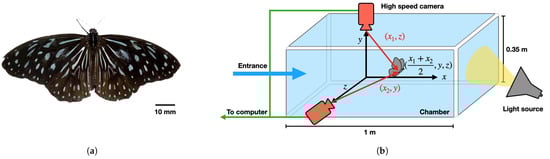
Figure 1.
Experimental setup. (a) Photograph of a blue tiger butterfly (T. septentrionis). (b) Measurement method. Two synchronised high-speed cameras were mounted onto a transparent chamber orthogonally along the y- and z-axis. By utilising the photographed images, a butterfly’s position could be determined.

Table 1.
Measured () and simulation model’s morphological parameters of the butterfly.
To capture the details of a butterfly’s body action, we utilised two high-speed cameras (Phantom v7.3 and v310, Vision Research, Wayne, NJ, USA). Both cameras were operated at 1000 frames per second with a resolution of 1024 × 1024 and placed outside a transparent chamber (size: 1 m × 0.35 m × 0.35 m) in which a butterfly could fly inside freely. As these cameras were placed orthogonally, we defined the direction from the chamber to the two cameras as y- and z-axis (see Figure 1b); the synchronised photographed films were examined to determine the angles between various body parts. To attract a butterfly to fly forward, we placed a light source on one side of the chamber. As the study focused on the flapping motion of forwarding flight, we abandoned the data for which the butterfly flew with turning. On counting the number of frames, we deduced the wingbeat frequency to be around 11.020 ± 1.076 Hz ().
To obtain the flapping kinetic equations, we utilised the coordinates measured from the experiments to rebuild them. Figure 2a shows the heading direction was determined by the body from to . The angle between the x-axis and was defined as the body pitching angle . Still, the vector was determined by the root and the wingtip ; the sweeping angle was obtained by calculating the complementary angle of the angle between and . Additionally, the wing plane was constructed with and (the direction pointing from to , with located on the trailing edge of the hindwing). Lastly, the wing rotation angle was computed from the normal vector of the wing (i.e., the direction of ) and ; the angle between the latter and the negative z-axis was defined as its flapping angle, where represents the axis of rotation. These parameters were utilised to describe the flapping flight behaviour of a butterfly.
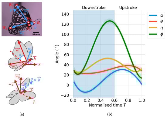
Figure 2.
Angle parameters of a flying butterfly. (a) Definitions of angles. From the coordinates of each feature’s points, body pitching angle , sweeping angle , rotation angle and flapping angle were obtained. (b) Angles measured from the experiments (). The solid lines indicate four feature angles; the surrounding shaded areas represent the 95% confidence intervals. The abscissa axis denotes the normalised time in a flapping period; the blue area (from to 0.6) indicates the downstroke phase, and the rest (from to 1) is upstroke.
Figure 2b shows the variation of the four angles in a flapping period measured from the experiments () with 95% confidence intervals (shaded areas). These curves were recognised as input parameters for subsequent simulation afterwards.
2.2. Computational Fluid Dynamics Simulation
To deduce the aerodynamic interactions that were hard to observe directly, we chose CFD simulation to generate highly accurate datasets. The obtained morphological parameters and kinematic equations were further utilised to build a butterfly model and regenerate the flight behaviour through a commercial solver (Fluent, Ansys, Canonsburg, PA, USA). The SIMPLEC algorithm was applied to resolve pressure and velocity fields [29]. To reduce the computational cost, we simulated the flow field under a relative condition frame. Therefore, the butterfly was flying at the centre of a sphere (see Figure 3a). The butterfly would thus encounter an incoming airflow with a virtual acceleration a created by its flight. To avoid inaccurate outcomes affected by the wall effect, the diameter of the spherical flow domain was set to (around 900 mm). As the Reynolds number of a natural flying butterfly is around –[30], the medium was considered an incompressible Newtonian laminar airflow, with a density of kg/m and viscosity of Pa·s. Furthermore, we utilised the following governing equations for computation:
in which u, t, p and g represent the velocity, time, pressure and gravity, respectively. The entire domain was split into two for giving different boundary conditions [29,31,32]. The front of the butterfly was considered to be the velocity inlet with an incoming flux accompanied by a. As a result, the stream fluctuated with the flight at each time step. The rear sphere was the pressure outlet. These conditions were defined as:
in which and indicate the unit vector along the x- and y-axis, respectively.
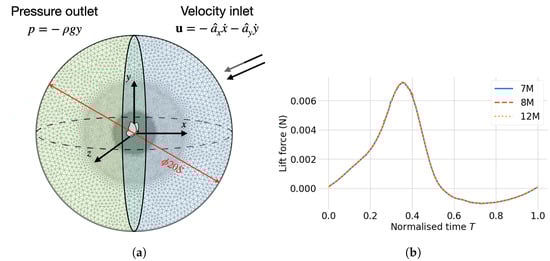
Figure 3.
Conditions of the simulation. (a) Boundary conditions (inlet: velocity, outlet: pressure). (b) Grid convergence test.
The grid size of the butterfly’s surface was 0.5 mm with a no-split condition (the air had zero velocity relative to the boundary), whereas its surroundings were set to 1 mm. This setting can enhance the precision of the simulation results [31,33]. We also utilised the lift force to do the grid convergence test. The result converged as the number of grids increased. Figure 3b illustrates the comparison among three different settings: the coarse grid (blue solid line, 7 million), the medium grid (red dashed line, 8 million) and the fine grid (amber dotted line, 12 million). From the result, we found that the maximum value difference between the coarse and fine settings was about 0.5% merely. Considering the balance between accuracy and computational cost, we hence selected the medium setting for the following computation.
We also chose the method of dynamic mesh (smoothing and remeshing) to prevent a negative mesh volume [34]. A flapping cycle was divided into 250 calculation time steps. The simulation outputs were the horizontal force , vertical force , normal force acting on a single wing and power consumption P at the 10th flapping cycle (stable flight). All these values were nondimensionalised by the following equation:
in which the wingtip velocity ; and were the corresponding untransformed forces and power. The Reynolds number of the simulation result was 6130, which was close to the experimental result of 6050.
As the study focused on the influence caused by amplitudes of body oscillation and wing rotation, we altered the simulated conditions of body pitching angle and wing rotation angle by multiplying them with scalers b and w. In total, 25 flapping data were collected (see Figure 4).
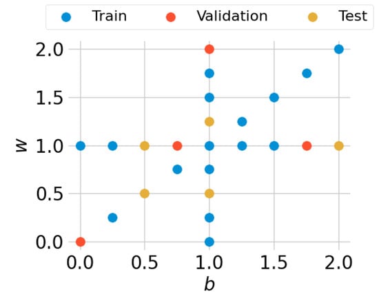
Figure 4.
Generated datasets. The data were randomly separated into training (64%, blue markers, ), validation (16%, red markers, ) and testing (20%, amber markers, ) groups. The testing data were merely utilised for evaluation and did not participate in the training processes.
3. Artificial Neural Network
An artificial neural network (ANN) is constructed by several connected computing cells (artificial neurons) inspired by the human brain as shown in Figure 5. The output y of the cell n can be calculated by the following equation:
in which are the input signals; ... are the respective weights; is the bias; and is the activation function (transfer function) [35]. The inputs were the scalers b and w. To increased the training performance, we normalised the values in the interval of [36]. On the other hand, instead of predicting 250 time steps for each aerodynamic property, we simplified it by fitting each parameter by a Fourier series:
where m is the order of the Fourier series. When choosing to fit the data, each aerodynamic property could be described by a vector formed by 11 parameters. We hence considered these 44 parameters (four aerodynamic properties, and P) as the output of an ANN model. As the number of outputs was shrunk from 1000 to 44, we could consider utilising a smaller number of hidden cells for the following calculation. The training process hence can be curtailed at the same time.
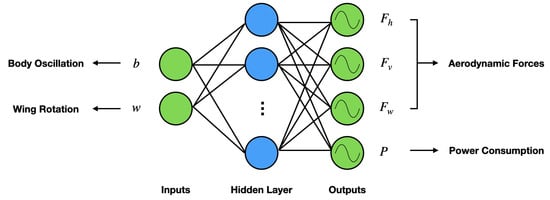
Figure 5.
Structure of an ANN model. The inputs were b and w, and the outputs were Fourier coefficients of and P.
Figure 6 shows two common activation functions utilised for neural networks. Recently, Rectified Linear Unit (ReLU) has been chosen as the activation function in various applications [37]. The function is defined by the formula:
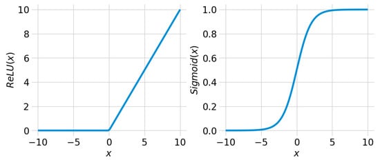
Figure 6.
Two types of activation functions.
Although the vanishing gradients problem is a critical issue when training an ANN, ReLU has a constant gradient of 1 when the input is greater than 0. Therefore, it is widely applied to ANNs. However, previous flapping wing studies chose the sigmoid function to estimate the mean values of aerodynamic coefficients [25,38]. The function can be described by:
As the s-shaped output of the sigmoid varies continuously in the interval of , the activation values hence do not disappear. Because we aimed to predict transient aerodynamic statuses rather than their mean values, we need to evaluate which function can provide precise estimations. We consequently constructed two models based on these functions and compared the results afterwards.
To train the model, we utilised Adam optimiser [39], an advanced backpropagation method [40], with the loss function of mean square error (MSE) to minimise the error. Although many studies [41,42,43,44,45] had proposed their rules of thumb to select the number of hidden units, the main idea is to improve the prediction accuracy and minimise errors. Therefore, we randomly picked up 80% of the data to train two types of models through a various number of hidden units iteratively. Among these datasets, 80% (i.e., 64% of the entire data) were utilised for tuning weights and bias; 20% (i.e., 16% of the entire data) were for validation. Considering the balance between accuracy and computational time, we have examined the loss when the number of hidden neurons was between 20 to 40. To avoid the setting merely benefiting specific cases, each training was repeated 30 iterations with the same settings but different training data selections. Figure 4 shows one of the random states that we have utilised. The learning rate and the epoch size were set to 0.001 and 60,000.
Figure 7 depicts the mean convergent curves of each case during the training process. From the testing result, we found that though the training loss of ReLU model kept decreasing when epoch size was greater than 10,000, the validation loss of it remained around . We further found that as the number of hidden units was 40, which had the smallest loss, its validation loss was and when epoch sizes reached 30,000 and 60,000. As the difference between these two values was less than 3%, we considered the 40 hidden neurons and 30,000 epochs to be an adequate setup. On the other hand, the training and validation loss of sigmoid model plots reveal that a larger number of hidden neurons did not promise a smaller loss. When the number of hidden units was 30, the validation loss difference between epochs 50,000 and 60,000 was less than 3% (epoch 50,000: , epoch 60,000: ). Consequently, we considered the number of hidden units and epochs to be 30 and 50,000, respectively.
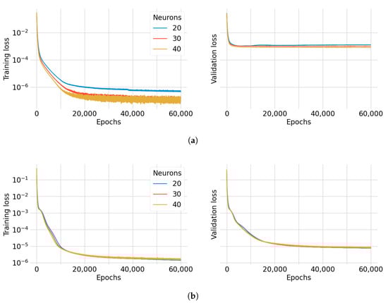
Figure 7.
Loss, the MSE of the 44 output parameters, of ReLU- (a) and sigmoid- (b) based ANN training processes.
It was unsure if the accuracy of the ReLU activation function was sufficient to predict the four aerodynamic properties, though the validation loss of the sigmoid-based model was even lower. We hence utilised both models for the following analysis. To avoid overfitting, the unused 20% of the data were assigned as testing datasets. As all the data generated by the CFD simulation were from the same system, the model that fits one group should fit the other as well. Because these cases were not utilised for previous training, they were considered to be unseen data for the following model evaluation. If the number of datasets is sufficient, we can utilise a large number of cases to evaluate our models. However, it is not easy to collect hundreds of results as it generally takes about 4 to 7 days to complete a single simulation. To deal with a limited amount of data, k-fold cross validation was implemented for obtaining a reliable evaluation [46]. To implement this method, the database needs to be randomly split into k groups first so that we can evaluate a model k times. In each iteration, we only utilise groups to train our network. As there is one group that does not join the training process, it can be utilised for testing. Therefore, this can be utilised to protect our models from overfitting as the model will be examined by k different combinations. To keep 20% of the entire data for testing, we chose k to be 5 in this study (see Figure 8).
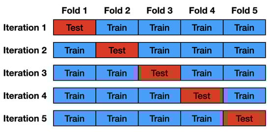
Figure 8.
k-Fold cross validation ().
4. Results and Discussion
4.1. Model Comparison
As the outputs of our models were coefficients of the four aerodynamic parameters, we converted the signal back by utilising Equation (8). The prediction can hence be compared with the original curves by calculating the coefficients of determination . The mean and standard deviation (SD) of the two models are given in Table 2. We first checked if the overtraining occurred on our model. Since the training and testing values are all close to 1, the models encountered neither underfitting nor overfitting problems. Although the MSE loss of the sigmoid-based model was smaller than the other one, as they both have mean values greater than 0.99, the differences were not obvious. However, the SD values of the ReLU-based model were slightly higher. The result implies that the sigmoid activation function generally provided higher precise estimations.
Table 2.
Statistics of the ReLU- and sigmoid-based models (mean ± SD).
As it is difficult to understand the difference between the two models by just viewing the values, we picked up a case from the testing group, which had a maximum value difference of 0.005, for comparison. Figure 9 presents the output aerodynamic properties as the b and w were assigned to 1 and 0, respectively. By comparing these curves, we can find that the red dashed line (sigmoid) almost overlaps with the black solid line (CFD simulation). On the other hand, the blue dashed line (ReLU) is slightly off in the peaks. By way of illustration, the blue dashed line shifted marginally to the right at in the -T plot. Nevertheless, the trends of four aerodynamic properties can still be identified.
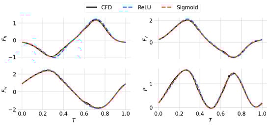
Figure 9.
Validation of the two models in comparison with the CFD simulation. The black solid lines were calculated by CFD simulation; the blue and red dashed lines were obtained from the ReLU- and sigmoid-based ANNs, respectively.
4.2. Aerodynamic Performance
While the traditional CFD simulation takes several days to complete a single computation, these two ANN models take less than a second merely. Due to the high , both methods achieve elevated estimation accuracy and can be implemented to accelerate the analysis process. The networks hence can be utilised to investigate the interactions between body oscillation and wing rotation behaviours. Owing to the limited payload, a MAV cannot carry a battery of substantial volume. Consequently, how to efficiently generate lift is a critical issue. We can hence utilise this neural network approach to optimise the flapping motion, such as searching the efficient flying kinematics.
In our study, the mean lift efficiency can be defined by:
where and are the mean values of and P in a single flapping period, respectively. We could hence obtain a quick result by utilising the ANN method. Figure 10 depicts the corresponding and when b and w are in the interval of [0, 2]. Because the two models presented similar outcomes, we only display the sigmoid-based calculation in Figure 10. The result illustrates that the maximum appears at . Nevertheless, the lift efficiency can still be improved by reducing w to 1.2. To verify if it fits the actual circumstance, we ran the simulation and compared the results (see Figure 11). The MSEs of and P were and , respectively. Considering the high and low MSE values, we believe this neural network approach can provide precise estimations which can be utilised for studying the flapping wing system.
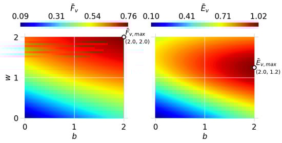
Figure 10.
Net vertical force and corresponding efficiency in a single flapping period.
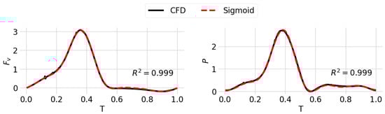
Figure 11.
Optimal aerodynamics obtained by the ANN in comparison with CFD simulated result.
Although it is still challenging to provide details such as flow fields with the current framework, we can utilise it to make a quick analysis and perform full CFD simulations of specific cases to clarify abnormal phenomena. This technique hence will be a great advantage when dealing with a complex system. Moreover, as we verified that the network could successfully estimate transient aerodynamic properties, we can extend the framework to include more complicated flapping motions as inputs in the future.
5. Conclusions
In this study, we introduce a novel neural network approach to speed up the transient analysis of flight mechanics. For evaluation, we analysed the butterfly’s flapping motions by CFD simulation and trained the model with these datasets. To simplify the model, we further utilised Fourier transform to reduce the number of neural cells. Through a series of tests, we found that both ReLU- and sigmoid-based models can accurately predict these coefficients, which can be utilised to obtain the original transient results. This enables us to rapidly estimate the corresponding aerodynamic properties with the given inputs.
The series of work conducted in this study aims to reduce the computational time cost. As the complex structure of flapping motion aerodynamics is non-linear, conventional approaches take excessive effort to analyse the unsteady system. With the aid of neural networks, we do not need to stick to CFD simulation for each case but can still obtain precise results without spending plenty of time. The technique reported here sheds new light on the development of flapping wing systems. This is a great advantage when a large amount of computing is required and provides us with a more efficient way to discuss the interactions among various parameters. Prior to this study, it was difficult to verify that the selected parameters were optimal. The technique introduced in the study makes it possible. We believe the framework will provide an efficient way to delve deeper into the flight mechanism and design a more efficient MAV.
Author Contributions
B.L. and Y.-J.L. conceptualised the research. Y.-J.L. and Y.-H.L. designed and performed the experiments. B.L. and C.-H.T. analysed the data. B.L. wrote the paper. J.-T.Y. administered the project and reviewed the paper. All authors have read and agreed to the published version of the manuscript.
Funding
The Taiwan Ministry of Science and Technology, grant number MOST 111-2221-E-002-123-MY3, funded this research. National Taiwan University partially supported this work under a project with contract NTU-CC-110L891401.
Conflicts of Interest
The authors declare no potential conflicts of interest with respect to the research, authorship and/or publication of this article.
Nomenclature
| a | Virtual acceleration |
| Aspect ratio | |
| b | Scaler of the body pitching angle |
| Mean chord | |
| Mean lift efficiency | |
| f | Frequency |
| Nondimensionalised horizontal force | |
| Horizontal force | |
| Nondimensionalised vertical force | |
| Vertical force | |
| Nondimensionalised normal force acting on a single wing | |
| Normal force acting on a single wing | |
| g | Gravity |
| k | Consecutive fold number |
| P | Nondimensionalised power consumption |
| p | Air pressure |
| Power consumption | |
| Coefficient of determination | |
| S | Wingspan |
| T | Normalised time |
| t | Time |
| u | Airflow velocity |
| V | Wingtip velocity |
| w | Scaler of the wing rotation angle |
| Rotation angle | |
| Sweeping angle | |
| Body pitching angle | |
| Air viscosity | |
| Air density | |
| Activation function | |
| Flapping angle |
References
- Fenelon, M.A.; Furukawa, T. Design of an active flapping wing mechanism and a micro aerial vehicle using a rotary actuator. Mech. Mach. Theory 2010, 45, 137–146. [Google Scholar] [CrossRef]
- Perez-Sanchez, V.; Gomez-Tamm, A.E.; Savastano, E.; Arrue, B.C.; Ollero, A. Bio-Inspired Morphing Tail for Flapping-Wings Aerial Robots Using Macro Fiber Composites. Appl. Sci. 2021, 11, 2930. [Google Scholar] [CrossRef]
- Rossi, M.; Brunelli, D.; Adami, A.; Lorenzelli, L.; Menna, F.; Remondino, F. Gas-drone: Portable gas sensing system on UAVs for gas leakage localization. In Proceedings of the IEEE SENSORS, Valencia, Spain, 2–5 November 2014; pp. 1431–1434. [Google Scholar] [CrossRef]
- Lan, B.; Kanzaki, R.; Ando, N. Dropping Counter: A Detection Algorithm for Identifying Odour-Evoked Responses from Noisy Electroantennograms Measured by a Flying Robot. Sensors 2019, 19, 4574. [Google Scholar] [CrossRef] [PubMed]
- Ellington, C.P. The aerodynamics of hovering insect flight. IV. Aerodynamic mechanisms. Philos. Trans. R. Soc. London. Biol. Sci. 1984, 305, 79–113. [Google Scholar] [CrossRef]
- Wakeling, J.; Ellington, C. Dragonfly flight. I. Gliding flight and steady-state aerodynamic forces. J. Exp. Biol. 1997, 200, 543–556. [Google Scholar] [CrossRef]
- Josephson, R.K.; Stevenson, R.D. The efficiency of a flight muscle from the locust Schistocerca americana. J. Physiol. 1991, 442, 413–429. [Google Scholar] [CrossRef]
- Dial, K.P.; Biewener, A.A.; Tobalske, B.W.; Warrick, D.R. Mechanical power output of bird flight. Nature 1997, 390, 67–70. [Google Scholar] [CrossRef]
- Nguyen, T.A.; Vu Phan, H.; Au, T.K.L.; Park, H.C. Experimental study on thrust and power of flapping-wing system based on rack-pinion mechanism. Bioinspiration Biomimetics 2016, 11, 1–16. [Google Scholar] [CrossRef]
- Sato, T.; Fujimura, A.; Takesue, N. Three-DoF Flapping-Wing Robot with Variable-Amplitude Link Mechanism. J. Robot. Mechatronics 2019, 31, 894–904. [Google Scholar] [CrossRef]
- Miyoshi, T.; Nishimura, T.; Shimizu, T. Handling parameters for rotational moment generation with four-wing flapping. J. Aero Aqua-Bio-Mech. 2018, 7, 1–8. [Google Scholar] [CrossRef][Green Version]
- Eldredge, J.D.; Jones, A.R. Leading-Edge Vortices: Mechanics and Modeling. Annu. Rev. Fluid Mech. 2019, 51, 75–104. [Google Scholar] [CrossRef]
- Lua, K.B.; Lee, Y.J.; Lim, T.T.; Yeo, K.S. Wing–Wake Interaction of Three-Dimensional Flapping Wings. AIAA J. 2017, 55, 729–739. [Google Scholar] [CrossRef]
- Zou, P.Y.; Lai, Y.H.; Yang, J.T. Effects of phase lag on the hovering flight of damselfly and dragonfly. Phys. Rev. E 2019, 100, 063102. [Google Scholar] [CrossRef] [PubMed]
- Lai, Y.H.; Ma, J.F.; Yang, J.T. Flight Maneuver of a Damselfly with Phase Modulation of the Wings. Integr. Comp. Biol. 2021, 61, 20–36. [Google Scholar] [CrossRef]
- Johansson, L.C.; Henningsson, P. Butterflies fly using efficient propulsive clap mechanism owing to flexible wings: Butterflies fly using efficient propulsive clap mechanism owing to flexible wings. J. R. Soc. Interface 2021, 18, 20200854. [Google Scholar] [CrossRef] [PubMed]
- He, Y.; Bayly, A.E.; Hassanpour, A. Coupling CFD-DEM with dynamic meshing: A new approach for fluid-structure interaction in particle-fluid flows. Powder Technol. 2018, 325, 620–631. [Google Scholar] [CrossRef]
- Fernandez-Gamiz, U.; Gomez-Mármol, M.; Chacón-Rebollo, T. Computational Modeling of Gurney Flaps and Microtabs by POD Method. Energies 2018, 11, 2091. [Google Scholar] [CrossRef]
- Cravero, C.; Marsano, D. Computational Investigation of the Aerodynamics of a Wheel Installed on a Race Car with a Multi-Element Front Wing. Fluids 2022, 7, 182. [Google Scholar] [CrossRef]
- Bagherzadeh, S.A. Nonlinear aircraft system identification using artificial neural networks enhanced by empirical mode decomposition. Aerosp. Sci. Technol. 2018, 75, 155–171. [Google Scholar] [CrossRef]
- Torregrosa, A.J.; García-Cuevas, L.M.; Quintero, P.; Cremades, A. On the application of artificial neural network for the development of a nonlinear aeroelastic model. Aerosp. Sci. Technol. 2021, 115, 106845. [Google Scholar] [CrossRef]
- Clawson, T.S.; Ferrari, S.; Fuller, S.B.; Wood, R.J. Spiking neural network (SNN) control of a flapping insect-scale robot. In Proceedings of the 2016 IEEE 55th Conference on Decision and Control (CDC), Las Vegas, NV, USA, 12–14 December 2016; pp. 3381–3388. [Google Scholar] [CrossRef]
- He, W.; Yan, Z.; Sun, C.; Chen, Y. Adaptive Neural Network Control of a Flapping Wing Micro Aerial Vehicle with Disturbance Observer. IEEE Trans. Cybern. 2017, 47, 3452–3465. [Google Scholar] [CrossRef] [PubMed]
- Goedhart, M.; Van Kampen, E.J.; Armanini, S.F.; de Visser, C.C.; Chu, Q.P. Machine Learning for Flapping Wing Flight Control. In Proceedings of the 2018 AIAA Information Systems-AIAA Infotech, Kissimmee, FL, USA, 8–12 January 2018; American Institute of Aeronautics and Astronautics: Reston, VA, USA, 2018. Number 209989. [Google Scholar] [CrossRef]
- Kurtulus, D.F. Ability to forecast unsteady aerodynamic forces of flapping airfoils by artificial neural network. Neural Comput. Appl. 2009, 18, 359–368. [Google Scholar] [CrossRef]
- Nguyen, A.T.; Tran, N.D.; Vu, T.T.; Pham, T.D.; Vu, Q.T.; Han, J.H. A Neural-network-based Approach to Study the Energy-optimal Hovering Wing Kinematics of a Bionic Hawkmoth Model. J. Bionic Eng. 2019, 16, 904–915. [Google Scholar] [CrossRef]
- Huang, H.; Sun, M. Forward flight of a model butterfly: Simulation by equations of motion coupled with the Navier-Stokes equations. Acta Mech. Sin. 2012, 28, 1590–1601. [Google Scholar] [CrossRef]
- Zhang, Y.; Wang, X.; Wang, S.; Huang, W.; Weng, Q. Kinematic and Aerodynamic Investigation of the Butterfly in Forward Free Flight for the Butterfly-Inspired Flapping Wing Air Vehicle. Appl. Sci. 2021, 11, 2620. [Google Scholar] [CrossRef]
- Lin, Y.J.; Chang, S.K.; Lai, Y.H.; Yang, J.T. Beneficial wake-capture effect for forward propulsion with a restrained wing-pitch motion of a butterfly. R. Soc. Open Sci. 2021, 8, 202172. [Google Scholar] [CrossRef]
- Senda, K.; Obara, T.; Kitamura, M.; Nishikata, T.; Hirai, N.; Iima, M.; Yokoyama, N. Modeling and emergence of flapping flight of butterfly based on experimental measurements. Robot. Auton. Syst. 2012, 60, 670–678. [Google Scholar] [CrossRef]
- Chang, S.K.; Lai, Y.H.; Lin, Y.J.; Yang, J.T. Enhanced lift and thrust via the translational motion between the thorax-Abdomen node and the center of mass of a butterfly with a constructive abdominal oscillation. Phys. Rev. E 2020, 102, 62407. [Google Scholar] [CrossRef]
- Lai, Y.H.; Chang, S.K.; Lan, B.; Hsu, K.L.; Yang, J.T. Optimal thrust efficiency for a tandem wing in forward flight using varied hindwing kinematics of a damselfly. Phys. Fluids 2022, 34, 061909. [Google Scholar] [CrossRef]
- Lai, Y.H.; Lin, Y.J.; Chang, S.K.; Yang, J.T. Effect of wing–wing interaction coupled with morphology and kinematic features of damselflies. Bioinspiration Biomimetics 2021, 16, 016017. [Google Scholar] [CrossRef]
- Suhaimi, S.; Shuib, S.; Yusoff, H.; Kadarman, A.H. Aerodynamic Performance of a Flapping Wing Inspired by Bats. Appl. Mech. Mater. 2020, 899, 42–49. [Google Scholar] [CrossRef]
- Zhang, Z. Artificial Neural Network. In Multivariate Time Series Analysis in Climate and Environmental Research; Springer International Publishing: Cham, Switzerland, 2018; pp. 1–35. [Google Scholar] [CrossRef]
- Sola, J.; Sevilla, J. Importance of input data normalization for the application of neural networks to complex industrial problems. IEEE Trans. Nucl. Sci. 1997, 44, 1464–1468. [Google Scholar] [CrossRef]
- Daubechies, I.; DeVore, R.; Foucart, S.; Hanin, B.; Petrova, G. Nonlinear Approximation and (Deep) ReLU Networks. Constr. Approx. 2019, 55, 127–172. [Google Scholar] [CrossRef]
- Thirumalainambi, R.; Bardina, J. Training data requirement for a neural network to predict aerodynamic coefficients. In Proceedings of the Independent Component Analyses. Wavelets, and Neural Networks, SPIE, Orlando, FL, USA, 21 April 2003; Volume 5102, p. 92. [Google Scholar] [CrossRef]
- Kingma, D.P.; Ba, J. Adam: A Method for Stochastic Optimization. In Proceedings of the 3rd International Conference on Learning Representations, ICLR 2015, San Diego, CA, USA, 7–9 May 2015; Available online: https://arxiv.org/abs/1412.6980 (accessed on 10 July 2022).
- Goh, A. Back-propagation neural networks for modeling complex systems. Artif. Intell. Eng. 1995, 9, 143–151. [Google Scholar] [CrossRef]
- Hornik, K. Approximation capabilities of multilayer feedforward networks. Neural Netw. 1991, 4, 251–257. [Google Scholar] [CrossRef]
- Boger, Z.; Guterman, H. Knowledge extraction from artificial neural network models. In Proceedings of the 1997 IEEE International Conference on Systems, Man, and Cybernetics. Computational Cybernetics and Simulation, Orlando, FL, USA, 12–15 October 1997; Volume 4, pp. 3030–3035. [Google Scholar] [CrossRef]
- Wang, S.C. Artificial Neural Network. In Interdisciplinary Computing in Java Programming; Springer: Boston, MA, USA, 2003; Volume 725, pp. 81–100. [Google Scholar] [CrossRef]
- Xu, S.; Chen, L. A novel approach for determining the optimal number of hidden layer neurons for FNN’s and its application in data mining. In Proceedings of the 5th International Conference on Information Technology and Applications, ICITA 2008, Cairns, QLD, Australia, 23–26 June 2008; Number ICITA. pp. 683–686. [Google Scholar]
- Sheela, K.G.; Deepa, S.N. Review on Methods to Fix Number of Hidden Neurons in Neural Networks. Math. Probl. Eng. 2013, 2013, 425740. [Google Scholar] [CrossRef]
- Cawley, G.C.; Talbot, N.L. Preventing over-fitting during model selection via bayesian regularisation of the hyper-parameters. J. Mach. Learn. Res. 2007, 8, 841–861. [Google Scholar]
Publisher’s Note: MDPI stays neutral with regard to jurisdictional claims in published maps and institutional affiliations. |
© 2022 by the authors. Licensee MDPI, Basel, Switzerland. This article is an open access article distributed under the terms and conditions of the Creative Commons Attribution (CC BY) license (https://creativecommons.org/licenses/by/4.0/).