Abstract
The objective of this study was to investigate the impact of varying wind speeds (1.5, 3.0, and 4.5 m/s), initial payload volumes (2 and 10 L), and nozzle droplet size characteristics (fine, medium, coarse) on drift during spray applications from an unmanned aerial vehicle (UAV) hovering freely in a wind tunnel. Along the length of the wind tunnel, glass slides were used to collect spray droplets at 14 points distributed in upwind, in-swath, and downwind distances. Analysis of the results showed that there are distinguishable shifts of up to 2 m in-swath as wind speed increases. Downwind of the UAV, a regression of the combined variables indicated that tunnel wind speed changed deposition the most overall, followed by nozzle/droplet size. Initial payload volume was less impactful. Overall, faster wind speeds, finer droplet sizes, and a heavier initial payload were associated with more drift on average. Wind directions and speeds were also measured on a finer scale of tunnel locations to record airflow pattern variability especially closer to the UAV. These findings may provide guidance to regulators and applicators to identify operating conditions for UAVs that limit off-target movement during applications.
1. Introduction
Many benefits and opportunities have been identified for pesticide application using unmanned aerial vehicles (UAVs), devices that are often termed drones. This includes potential for precision applications that use GIS-enabled technology, integration with crop monitoring devices that facilitate treatment of areas with high pest infestation rates, reduced worker exposure, ability to make applications in complex and hilly terrain thereby contributing to safety of pilots in fixed wing and other aircraft, night applications, rapid rates of application and field coverage, and potential for reduced spray drift due to the ability of UAVs to fly close to crop canopies [1].
While the potential for UAV pesticide application appears great, pesticide labels in the US and other countries do not routinely specify UAV use for application [1,2,3]. Because of this, UAV use for pesticide application remains limited. The lack of supporting regulations may be explained by the newness of UAV pesticide applications and the rapid evolution of this technology. In the US, regulating UAVs for crop protection under the Federal Insecticide Fungicide and Rodenticide Act (FIFRA) requires a multistep process including development of a certification process for applicators, updating pesticide labels, developing an appropriate risk assessment paradigm, defining agricultural (ag) versus non-ag uses, and amending laws and regulations, etc. [4]. This regulation process is currently ongoing [1]. Furthermore, to appropriately assess human and ecological risks of UAV-based pesticide application, the magnitude and extent of the associated spray drift must be determined [3]. Off-target drift may be a source of exposure to bystanders, residents, operators at the application, to nearby waterbodies, as well as a threat to crops in adjacent fields where there is high sensitivity to selected herbicides.
While traditional application technologies, such as fixed-wing aircraft, tractor-mounted booms, and airblast sprayers, are also at risk of off-target drift, the processes which contribute to pesticide spray drift using these technologies have been intensively studied and are characterized in the well-known AgDRIFT® model [5]. The model serves as a core resource to risk assessments that evaluate potential spray drift exposures. Currently, the model (version 2.1.1 [6]) is not configured to describe spray drift from UAV pesticide applications. To meet this need, research is needed to characterize and understand spray drift behavior under conditions commensurate with UAV use and type. How factors such as downwash from multi-rotor vortices, spray nozzle orientation and type, vehicle height above the crop canopy, air speed and wind patterns on spray droplet size or movement, as well as their interactions, require investigation. To understand these factors, both field and laboratory-based studies are needed. Field studies offer the most realism but are often constrained by environmental conditions such as the range of wind speeds on a given day. There are many published reports that can serve as a resource [7,8,9,10,11,12,13,14,15,16,17,18].
Recent research conducted under laboratory or wind tunnel conditions have described droplet dispersion patterns associated with UAV spray applications. Wang et al. [19] reported on the spray drift potential of three nozzle types, flat fans with fine and very fine spray qualities, hollow cones which produced very fines spray, and air induction nozzles with medium, coarse and very coarse droplet characteristics. The authors observed that the air induction nozzles showed the greatest potential to attenuate drift. In that study, a single unit of quadrotor UAV was used. Similarly, Wang et al. [20] examined factors that were important to increased drift during a UAV spray application and concluded that spray droplet characteristics or spray quality and wind speed are influential factors to consider during UAV spray applications. In that study, the working length of the wind tunnel was approximately 8 m and the UAV was affixed to a horizontal bar in the wind tunnel, which likely limited the natural attitude of the UAV while in operation. Yang et al. [21] used CFD modelling to examine the dynamics of downwash from a six-rotor UAV and droplet movement and distribution. They showed that increased payload and lower operating height increased the in-swath deposition.
Zhan et al. [22] varied the operation height and payload of a four-rotor UAV and found that an increase in operating height correlates with a decrease in downwash airflow velocity and drift potential increases with higher payload. Ambient wind speed varied from 0.83 to 2.87 m/s, and it is unclear the influence the ambient wind speed had on the drift in that field study.
Laboratory studies offer useful alternatives where key variables can be more rigorously controlled. In these investigations, the UAV is typically mounted on a track [23,24,25,26] or secured in a wind tunnel [19,27]. Wind tunnel studies are constrained for UAV testing by loss of the forward vector, and typically there is a height restriction. However, laboratory studies have the advantage of full control of wind conditions and the ability to test potentially sensitive variables, such as rotor thrust. Because of these advantages, laboratory studies still provide useful information to supplement the regulatory process.
In the current investigation, we evaluated spray drift potential from a commercial UAV with four under-rotor nozzles in a wind tunnel housed in a utility building. The UAV was loosely secured within a frame using oversized U-bolts, so that it could produce its own rotor thrust to maintain hovering altitude at the programmed height within the air flow. This allowed simulating behavior in an outdoor spraying scenario with the exception that the forward (across wind tunnel) vector was not included. Spray drift deposition was measured along the swath at three wind speeds with three different flat-fan nozzle types, representing fine, medium, and course droplets, and with two payloads. This factorial experiment was designed to identify how these variables contribute to spray drift, both individually and together.
2. Materials and Methods
2.1. Wind Tunnel and UAV Setup
The main experiment was conducted in an ambient wind tunnel with a width of 4.4 m, a height of 2.5 m, and an overall working length of approximately 49 m with 42 m downwind of the application zone. A filter wall was located at the downwind end of the tunnel, and a mixing baffle and a uniformity baffle were located upstream of the application zone to help ensure homogenous airflow. The low-speed wind tunnel operated at an average of 6% turbulence at the application zone at wind speed ≤ 4.5 m/s, with turbulence decreasing with distance (Table A1).
The DJI Agras MG-1P UAV was used in this study since at the time of the experiment it was the latest release for the MG platform from DJI that was widely available and supported in the US market. The Agras MG-1P is an octocopter UAV designed for precision variable-rate application of liquids, allowing selectable levels of spray rate and efficiency using DJI smart flight mode.
For this experiment, the UAV was allowed to hover freely in a 90° crosswind orientation, contained on its upward fuselage, within four vertical U-bolts connected to ceiling support beams (Figure 1). The U-bolts were of equal length (0.32 m) and sufficient to clear the support arms and allow free movement of the UAV within the upward span. While in flight, the center of the U-bolts equated to a spray height of 1.5 m above the ground. The rotors were 0.33 m above the nozzles. The U-bolts were placed inward enough to avoid contact with the rotors while the UAV was tilted in a 4.5 m/s wind and high enough to avoid contact with the spray from the upwind nozzles.
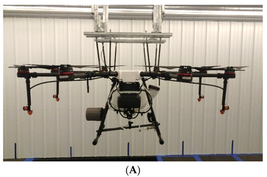
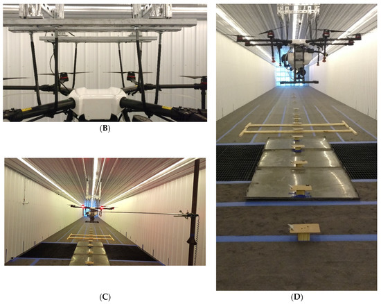
Figure 1.
U-Bolt containment system allowing lightly confined flight. (A) UAV oriented to spray perpendicular to the airflow—front-facing view, (B) Closeup of U-bolts, (C) Setup showing the hot wire anemometer, (D) View from upwind of the wind tunnel. The DJI Agras MG-1P is configured with 4 nozzles, mounted beneath the rotors, visible as red attachments in photo A.
The purpose of this tethering system was to maintain the position of the UAV/sprayer without interfering with either its flight mobility or the nozzle spray pattern. This system also enabled the sprayer and nozzles to adopt a realistic flight angle corresponding to the wind speed. The flight path/direction was oriented perpendicular to the wind direction. The rotors were unobstructed and able to operate as normal, thus typical downward vortices were generated. Spray nozzles were positioned 1.5 m above the tunnel floor, which was covered with absorbent pads to prevent droplet bounce.
2.2. Study Design
The main portion of the study consisted of running spray drift tests on all combinations of three nozzles, three wind speeds, and two initial payloads, described below.
Three nozzle types representing fine, medium, and coarse sprays were tested, described below in the nozzle characterization section. For each test, four nozzles of one type were fitted to the UAV, one under each of the side rotors (Figure 1A). Their calibration to the same flow rate and pressure ensured comparability of droplet size and transport across nozzle types.
Wind speeds of 1.5, 3.0, and 4.5 m/s were evaluated. The fastest speed of 4.5 m/s corresponds to approximately 10 mph, often listed as a maximum label wind speed for pesticide ground spray applications. These wind speeds covered a reasonable range of application conditions and served as a key variable to test in the wind tunnel.
The initial payload of the UAV was the final study design variable, tested for potential effect by starting each run with a full tank (approximately 10 L) and with a near-empty tank (approximately 2 L). Both fill levels were marked on the tank for consistency across tests, and the combined mass of the UAV and spray material was measured at both fill settings (Table A2). This variable was included to test for any potential effect of rotor thrust, due to the overall weight, on application quality.
All combinations of these three variables produced 18 unique experimental conditions. With three replicates each, 54 tests were run. Testing was performed in a randomized sequence to minimize bias due to any variation in ambient testing conditions.
The spray solution, consisting of water and a tracer dye, fluorescein sodium salt (CAS Number: 518-47-8), was concentrated at 10 g (dye)/L (water).
2.3. Experimental Setup and Procedure
Deposited spray droplets were collected on fourteen glass slide samplers placed upwind of the application (−3 and −2 m), within the swath of the spray (−1, 0, and 1 m), and at 9 downwind distances from the UAV (2, 3, 4, 5, 6, 8, 12, 16, and 20 m; Figure 2). Each glass slide sampler consisted of two 2.5 × 7.5 cm glass slides (Fisher Scientific, Hampton, NH, USA. Cat. No. 12-544-4), raised approximately 7.6 cm off the ground to prevent ground air turbulence or bounce from reaching the slides (see Figure A1 for photo). The slides were aligned down the approximate center of the tunnel.
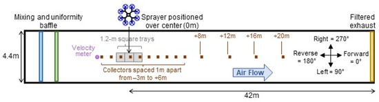
Figure 2.
Diagram of the experimental setup in the wind tunnel. Glass slide samplers are shown from −3 m to 20 m, with three trays in-swath. Directions on the right correspond to those recorded by the 3D anemometer. Drawing not to scale.
Additionally, to capture on-target deposition in the swath of the spray, three 1.2 × 1.2 m low-profile catch trays were installed immediately below the UAV, one centered at each of the −1, 0, 1 m reference points (see Figure A1 for photo). The glass slide samplers that shared these three locations were placed in the center of these trays. The tray volumes were not intended to comprehensively capture all in-swath drift from the UAV but can allow for relative comparisons.
During each test, the wind tunnel was allowed to stabilize to the target wind speed before each spray, the UAV hovered within its tethering system to achieve a release height of 1.5 m, and the sprayer was programmed to run for 30 s at a flow rate of 0.3 L/min per nozzle, releasing a total of approximately 606 mL per test. After this, the UAV was turned off and tunnel airflow continued for approximately two minutes to allow the droplets to settle. Tray volumes were recorded after each run. The glass slide samplers were collected and stored in a cooler, followed by a −20 °C freezer until they were shipped in a cooler to the laboratory. There, they were placed in a −20 °C freezer and defrosted prior to analysis.
2.4. Sample Analysis
The fluorescent dye residues were extracted from the glass slides with 20 mL of 10% methanol in 0.01 N NaOH (aqueous). The extraction solution was added to each 50-mL conical tube containing two glass slides and placed on a rotary-bed shaker for 15 min at 200 rpm. Extracts were analyzed with a Molecular Devices SpectraMax i3 fluorimeter with excitation at 485 nm and emission at 535 nm. The mass of the dye recovered was computed by dividing measured concentrations (in ng/mL) by dilution factors and multiplying by extraction volumes (in mL). Masses were converted to ng/cm2 by dividing by the area of the two glass slides (2 × 2.5 cm × 7.5 cm = 37.5 cm2). All samples exceeded the limit of quantitation of 0.005 ng/mL for the fluorescein dye.
2.5. Nozzle Characterization
Three flat-fan spray nozzle types were evaluated in this study: TeeJet Extended Range (XR) 11001 representing fine droplets, Turbo TeeJet (TT) 11001 representing medium droplets, and Lechler air-injected IDK 120-01 representing coarse droplets. Prior to the main experiment, these nozzles were calibrated to determine flow rate and swath width at a release height of 1.5 m. The target flow rate was 0.3 L per minute for each nozzle (30 psi). This calibration ensured uniformity of the spray pressure, flow rate, application rate, and downwash/vortex patterns across nozzles, for the duration of the experiment.
To define differences among nozzles, they were evaluated using two different instruments. First, a Malvern Spraytec device (Malvern Instruments, Worcestershire, UK) quantified the droplet size distribution (DSD) of each nozzle. The nozzles were aligned such that the sprayed droplets were parallel to the wind direction (downwind) while traversing the laser beam. Wind speed was set to 4.5 m/s and three replicates were run. Means across replicates were calculated by nozzle. The spray quality classification is based on ISO 25358 [28].
Second, an Oxford Lasers VisiSize P15 instrument was used to measure whether the DSDs varied when the UAV rotors were off, compared with the UAV hovering with 2-L and 10-L payloads. This instrument results in a spatial distribution, similar to the Malvern Spraytec, but also records the droplet velocities. In all cases, the Oxford laser traversed through the plume at a slow rate until at least 25,000 droplets had been measured. Spray droplets were measured approximately 20 cm below one of the under-rotor nozzles, and each nozzle was tested with three replicates. For the 2-L payload tests, droplets were measured until the tank was empty. The 10-L fill was sprayed until approximately half of the tank remained. The tests were repeated for each nozzle, with droplet diameters recorded.
A two-way ANOVA test and Tukey post-hoc test were run on the resulting Dv50 values to test for potential effects from the nozzles as well as the rotor condition. Data were determined to be normal with homogenous variance, and all analyses were completed in R software (Shapiro–Wilk test and Bartlett test p values each > 0.01; [29]).
2.6. Meteorological Measurements
Meteorological conditions in the tunnel were monitored during the experiment using a Velocicalc® Air Velocity Meter (TSI model 9565-P). This portable, handheld unit measured temperature, relative humidity, and wind speed. The instrument was located just upwind of the −3 m sampler at 1.5 m height and centered in the tunnel. Measurements were taken at a frequency of 1 Hz, with values averaged over 1 min: 15 s prior to testing, the 30-s application, plus 15 s after application.
2.7. 3D Anemometer Measurement on a Grid across Tunnel
Since the UAV produced its own downdraft, it introduced variability in air movement into the otherwise controlled setting of a wind tunnel. To examine the resulting wind scape created by this setup, 3D anemometers (R.M. Young, Traverse City, MI, USA. Model 81000 Ultrasonic Anemometer) were used to measure wind speeds and directions at multiple distances, heights, and widths in the tunnel. The purpose of this effort, carried out separately from the main spray drift experiment, was to better understand wind directions and velocities, if they varied in the tunnel.
A cross-section of the tunnel was defined by three tunnel widths (left, center, and right) and three tunnel heights (bottom, middle, and top), defining nine points at which wind measurements were taken (Figure 3). The UAV’s rotors nearly aligned with the top height (below by 7.5 cm), and the spray release height was 1.5 m, approximately halfway between the top and middle points. The UAV’s 1.92-m width nearly spanned the distance between left and right points (18 cm away from each). This 3 × 3 cross-section of measurement points was repeated at each of the 14 distances where glass slide samplers were placed along the tunnel length (−3 m to 20 m, with the exception of top heights at and adjacent to the UAV distance and the middle center height at the UAV distance).
Figure 3.
Cross-section of tunnel showing wind measurement locations using the 3D anemometer. Wind was measured at nine points on a plane defined by three heights (Z dimension) and widths (X dimension). These nine points were measured at each of the 14 distances (Y dimension) shared by the glass slide samplers. The UAV’s height and width relative to these points are marked in green. The view is from the far downwind end of the tunnel, facing upwind towards the UAV. Drawing not to scale.
At each point, wind speeds in the X (left to right), Y (upwind to downwind), and Z (bottom to top) dimensions were measured (Figure 3). Direction was also recorded in degrees, with the anemometer oriented such that a 0-degree measurement represented the dominant wind tunnel direction on a plane parallel to the floor (degrees labeled in Figure 2). The effort was repeated at the three nominal tunnel wind speeds, and with the UAV in a hovering position and at the two payloads. The sprayer was not on during this portion of the study.
Each run lasted 60 s, with a measurement taken every 1/32nd of a second. Wind speed measurements were averaged over this time to result in one value per location, dimension, and run. The direction measurements were first converted from polar to cartesian coordinates, then averaged (details in Table A3). On the tunnel cross-section, X- and Z-dimension velocities were combined using the same process (using arctangent function atan2, [29]) to estimate an angle at each measurement point. Wind speeds were aligned with the directions by calculating the hypotenuse of mean X and Y wind speeds (), as well as the mean X and Z wind speeds. For these values to be graphed, angles had to be translated from the conventional meteorological plane to the standard math coordinate plane. Values were graphed, comparing the wind speed and payload tests.
2.8. Statistical Analysis of Downwind Deposition
Multiple linear regression was used to generate deposition curves downwind of the UAV (distances 2–20 m) and to statistically test for differences among the nozzles, wind speeds, and payloads. Mass per area of fluorescein dye measured on glass slide samplers (in ng/cm2) was the dependent variable, transformed by natural logarithm for linearity and homoscedasticity. The main independent variables tested were distance (in m, also transformed by natural logarithm), nozzle as a categorical dummy variable, wind speed tested both as a categorical variable and as a continuous value (in m/s), and payload as a categorical variable. Graphing of residuals informed the transformations as well as testing of the variables for interactions.
Additionally, meteorological variables from the handheld instrument were tested as covariates to check for their potential to affect spray drift patterns in the tunnel. Mean relative wind speed was calculated as the difference between the target and mean of measured wind speeds, allowing for its use in statistical testing without confounding with the nominal wind speed. Measured wind speed was also tested as an alternative to the target wind speed. Temperature, humidity, and relative wind speed were all correlated: runs with cooler temperatures also had higher humidity and faster wind speeds (Figure A2). Due to this collinearity, they were tested separately and as an interaction variable of relative wind speed × relative humidity/temperature, in recognition of temperature’s inverse correlation to the others.
The 3D anemometer data were aligned with the data from the main spray drift experiment to match distances, nominal wind speeds, and payloads. Though these anemometer measurements were collected during a separate effort, they contributed a unique value by informing how wind varied across distances in the tunnel. In addition to using measurements along the center line of the tunnel as covariates, velocities at the left and right were averaged to represent wall effects. The X, Y, and Z dimensions as well as bottom, middle, and top heights were each kept separate. Each of these variables was centered by subtracting their mean value within the design structure of nominal tunnel wind speeds and payload, to prevent their multicollinearity (see Figure A3 for more detail). Since comparison among these centered anemometer variables revealed frequent correlation, only one was tested at a time in the regression.
All analyses were completed in R software [29] using the package ggplot2 [30] for graphs. One low outlier was excluded at the farthest distance (see Figure A4), resulting in the regression being run on 485 points. Assumptions of normality, homoscedasticity, linearity of residuals, and lack of multicollinearity were checked graphically and with variance inflation factors [31].
3. Results
3.1. Nozzle Characterization
The DSD analysis performed resulted in average droplet sizes listed in Table 1. The ranking based on volume mean diameter shows Lechler IDK 120-01 (coarse) > TT11001 (medium) > XR11001 (fine) at the three evaluated percentiles of the distribution. Consequently, the XR11001 (fine) nozzle produced the largest fraction of driftable fines (i.e., droplets diameter ≤ 141 µm [32]).

Table 1.
Average droplet size spectrum for each of the 3 nozzles at 30 psi, determined using the Malvern Spraytec instrument. Dv10,50,90 = 10, 50, 90% of spray volume contains droplets smaller than the specified diameter, respectively.
Measurements taken from the Oxford Lasers instrument showed that the Dv50 values of all nozzles were statistically different from one another (ANOVA p < 0.0001), with the coarse nozzle greater than the medium by 172 μm and the medium greater than the fine by 158 μm on average (Figure 4). Though the difference between the two payloads’ Dv50 values was insignificant when the rotor was on (Tukey p = 0.99), Dv50 was smaller when the rotor was off (ANOVA p = 0.0053).
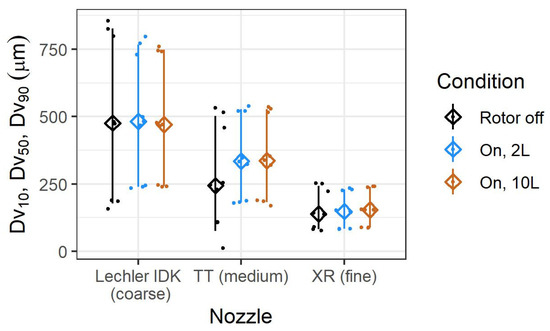
Figure 4.
For each nozzle and condition, diamonds show mean Dv50, and whiskers extend from mean Dv10 to mean Dv90. Small points show replicate values. Data were collected using the Oxford Lasers instrument.
However, as visible in Figure 4, this reduction associated with the rotor was solely driven by the medium nozzle. Without it, the rotor condition was insignificant (ANOVA p = 0.309). Using medium nozzle data only, the Dv50 diameter was 92 μm smaller on average when the rotor was off compared with when it was on at either payload (Tukey p = 0.0005). The medium nozzle’s distribution was also more asymmetrical, since its Dv90 was similar to that of the other rotor conditions. The dominant significant result was therefore the difference among nozzles; to a lesser extent, the rotor condition only changed the Dv50 for the medium nozzle.
3.2. Meteorological Data Summary
During the main experiment testing UAV spray drift in the tunnel, temperature, relative humidity, and wind speed were measured and are summarized in Table 2. Temperature varied from 23 to 33 °C across all tests, while humidity had a wider range from 44 to 91%. Actual measured wind speeds had slightly higher means than their target, e.g., the 1.5 m/s nominal runs had a mean of 1.60 m/s, and overall ranged from −0.17 to +0.20 m/s around their target. These variables were tested for potential impact to results as part of the downwind regression below.
Table 2.
Summary of meteorological conditions measured in the tunnel.
Variability in meteorological conditions was also checked alongside the study design variables (graphed in Figure A5). The Lechler IDK nozzle runs were carried out on the final day of the experiment, and the 2-L runs occurred in warmer, drier tunnel conditions with slower relative wind speeds than the 10-L runs with this nozzle. Otherwise, conditions were often similar among sets of replicates, but generally varied across nominal wind speeds and nozzles.
3.3. Upwind and In-Swath Deposition
Beneath the UAV, fluorescein dye was collected on glass slides (measured as mass per unit area) as well as in 1.2-m square trays (measured as volume). Results from both substrates are shown in Figure 5, focusing on distances 3 m upwind and downwind of the UAV to observe the swath width.
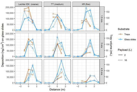
Figure 5.
Collected tray volumes and glass slide deposition under the UAV (−3 m to +3 m) as it varied by nozzle, nominal tunnel wind speed (m/s), and initial payload, as labeled. Points mark the mean values of three replicates.
The most consistent trend was associated with nominal tunnel wind speed: as the speed increased, spray shifted towards the downwind direction (higher points shifted right from top to middle to bottom rows in Figure 5). This swath displacement was <1 m to 2 m, observable in glass slide and tray data, and for all nozzles. The greatest upwind values, e.g., at −1 m, therefore occurred at the slowest wind speed, and vice versa.
Differences among nozzles were distinguishable among tray volumes. The coarse nozzle resulted in the largest collected volumes at these in-swath distances, when comparing within all wind speeds. Conversely, the fine nozzle had the least collected volume since the spray was more susceptible to drift. However, glass slides did not capture a consistent pattern among nozzles (e.g., the opposite occurred at 1.5 m/s, where the fine nozzle had the most deposition). The reason for this is unclear but may be due to the trays covering a much larger area than the glass slide samplers (1.4 m2 vs. 0.00375 m2).
The two initial payloads tested produced comparatively different depositions in tray volumes, depending on the nozzle. The 10-L payload had more volume with the medium nozzle, but less volume with the coarse nozzle. Meteorological conditions may have been a factor in these results. Larger droplets may be more likely to be driven downward by greater thrust for higher payload, whereas smaller droplets may be more likely to drift. Differences were inconsistent among sets in glass slide data.
Particularly low glass slide deposition was measured with the fine nozzle at 4.5 m/s (bottom right panel in Figure 5). For example, the 2-L payload value at +1 m was 4× less than the next-highest value at any other nozzle–speed combination at that distance. The fine droplets appeared to have drifted farther downwind at this fast speed, as examined in the next section.
3.4. Downwind Deposition
Downwind deposition of fluorescein dye on glass slides, defined from 2 to 20 m from the UAV, is graphed distinguishing among nozzle, wind speed, and payload in Figure 6. Variability in this deposition was quantified in a regression defined by distance, nozzle, nominal tunnel wind speed, initial payload, meteorological condition, and downward wind speed measured from the 3D anemometer. This regression explained 80.0% of deposition variability in this experiment (adjusted R2), with residual errors shown in Figure 7. Details are shown in Table 3 and described in this section.
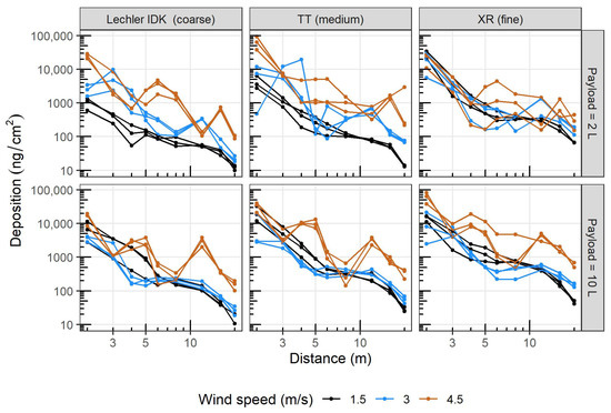
Figure 6.
Downwind deposition of fluorescein dye on glass slides in all runs in the wind tunnel. Plots are split by nozzle and payload as labeled, with colors distinguishing nominal tunnel wind speeds. Lines connect measurements within replicates.
Figure 7.
Predicted vs. measured deposition values, labeled by nozzle and colored by nominal tunnel wind speed. The line is at 1:1, such that points above are overestimates and under are underestimates.
Table 3.
Results of regression describing ln(deposition in ng/cm2) on glass slides from 2 m to 20 m downwind of the UAV. The equation is in the form: . The base model has 1.5-m/s wind speed, the coarse Lechler IDK 120-01 nozzle, and 2-L payload; therefore, these levels do not have coefficients and do not appear in the table. These results are also written as equations in Table A4.
Keeping all other variables constant, each 10% increase in distance from the UAV resulted in a 16% decrease in deposition on glass slides on average (Table 3; (1.10−1.870) − 1 = −0.163). This relationship reflects the logarithmic shape of the deposition curve.
Nozzles had significantly varied deposition amounts (ANOVA p value < 0.0001, Table 3) in that the coarse Lechler IDK 120-01 produced 55% less deposition than the medium TT11001 on average (exp(−0.793) − 1 = −0.547), which in turn produced 31% less than the fine XR11001 on average (exp(0.793−1.171)−1 = −0.3148; both p values < 0.0001). These differences are visualized in Figure 8A, in which all other variables in the regression were kept constant.
Figure 8.
Mean differences of downwind fluorescein dye deposition shown one variable at a time, as labeled. Confidence intervals of 95% are shaded around each level. Within each plot, all other variables were kept constant; these constant values were 3.0 m/s wind speed, 2 L payload, medium TT11001 nozzle, the mean of the meteorology variable (0.181), and mean of the centered 3D anemometer variable (0 m/s). Percentage differences within variables are the same regardless of other variables’ values. Further explanation is in-text.
Varying the wind speed in the tunnel resulted in the greatest differences in deposition, among all variables tested in this experiment. These differences varied by distance, since both the intercepts and slopes were significantly different (all ANOVA p values < 0.0001; Table 3, Figure 8B). All else constant, at 2 m, the middle wind speed had 43% less average deposition than the other two. However, this 3.0-m/s speed’s deposition was very similar to that of the 1.5-m/s average at 4 m, where both were less than the 4.5-m/s value by 62% on average. At the farthest distance of 20 m, all wind speeds’ mean depositions diverged such that 1.5 m/s produced 72% less than 3.0 m/s, which in turn produced 87% less deposition than 4.5 m/s. More spray therefore drifted farther when the UAV was flown in faster tunnel winds. Additionally, residual errors were smallest at 1.5 m/s and greatest at 4.5 m/s (based on standard errors, wider span of orange points in Figure 7, and wider confidence interval in Figure 8B). This suggests that more variability in deposition occurred during this higher wind speed, possibly due to greater propagation of downwash airflow turbulence.
Operating the UAV starting from different fill levels resulted in significant deposition differences relatively smaller than those produced by wind speed or nozzles (Figure 8C, intercept p < 0.0001 and slope p = 0.0195). At 2 m from the UAV, a near-empty 2-L payload produced 48% less deposition on average compared with the full 10-L payload, but this difference shrunk to 10% at 20 m. The effect of payload size was therefore more pronounced at closer distances.
The quantification of effects associated with these three study design variables (nozzle, nominal wind speed, and payload) was refined by controlling for the relatively small variation in meteorological conditions that occurred in the tunnel over the duration of the study. The interaction variable of relative wind speed × relative humidity/temperature was statistically significant in the regression, though relatively the least so (p = 0.0061, Table 3), reflected in the smaller differences visible among the lines in Figure 8D. The graphed lines were drawn using the interaction variable’s 5th percentile (“Warm, dry, slow”), its mean, and its 95th percentile (“Cool, moist, fast”). The 5th percentile deposition was less than the 95th percentile by 36% on average. By comparison, relative wind speed (ranging only by 0.4 m/s) was the only variable of the three that was significant on its own (p = 0.0181, not in final regression), suggesting that it drove most of the association. Therefore, faster wind speeds, co-occurring with cooler and more humid air, were associated with more deposition on average.
The 3D anemometer variable was the final covariate in the regression, also serving to refine and isolate the effects of the study design variables. Among the centered 3D anemometer speeds tested (different dimensions and cross-sectional location in the tunnel), the strongest was the Z dimension at the center width and bottom tunnel height (p < 0.0001). A negative speed, indicating a downward direction from the UAV to the floor, was associated with more deposition at that distance. On average, an increase in Z-dimension speed by 1 m/s, including potentially changing from downward to upward direction, decreased deposition by 82% on average (exp(−1.689) − 1 = −0.815). This variable had a 1.6 m/s range, centered relative to its mean within payload and nominal tunnel wind speed (more detail in Figure A3).
In Figure 8E, lines were drawn to show 5th percentile, mean, and 95th percentile Z dimension speeds, which were calculated unique to each distance. This was the only variable that informed change over distance, and as such, notably improved the shape of the regression’s residuals by partially explaining the nonlinear patterns visible in Figure 6 (improvement to residuals shown in Figure A6). The fastest downward speeds occurred close to the UAV. Though distances of 2, 3, and 12 m had a wider range of downward speeds from one trial to the next, more consistency was measured at 4, 5, 16, and 20 m. By using this 3D anemometer as a covariate in the regression, this source of tunnel variability was controlled for, and can be set to its mean (0 m/s) in the equation to better isolate and understand the study design variables of interest, as it was in Figure 8A–D.
Overall, the combination that produced the most drift deposition on average had the fastest wind speed of 4.5 m/s, the fine nozzle, and the 10-L payload. For perspective, this highest-deposition scenario resulted in an average of 1741 ng/cm2 at 20 m, which is 97× higher than the 18 ng/cm2 average from the lowest-deposition scenario of 1.5 m/s, coarse nozzle, and 2-L payload (calculated using the mean of the meteorology and 3D anemometer variables in the regression formula). At the closest distance of 2 m, this highest-deposition scenario was 6× greater than the lowest-deposition scenario on average. Examples of high-, medium-, and low-deposition scenarios’ actual and predicted values are graphed in Figure A7.
3.5. Wind Direction and Airflow Variability
Though the wind tunnel was large enough to accommodate the UAV, its operation caused disturbances in the airflow at the walls which influenced the deposition downwind. Without the UAV, the wind direction was always predominantly in the downwind direction (up to 6% turbulence, Table A1). When the UAV was in operation, wind directions measured from the 3D anemometer at multiple locations in the tunnel elucidated the resulting variability in air flow.
Results are shown as arrows on a plane parallel to the floor in Figure 9A, with combined X–Y velocity in color. Perpendicular to this diagram is Figure 9B, showing air movement in the cross-section of the tunnel with X–Z velocity at the 2 m distance. This example figure is based on measurements during 4.5 m/s tunnel air flow and with a UAV payload of 10 L, with the remaining combinations in Figure A8. Overall, deviation from the dominant direction was most common at distances near the UAV, and the direction of air flow generally became more streamlined farther downwind (Figure 9A and Figure A9).
Figure 9.
Wind direction and velocity measured using the 3D anemometer, with nominal tunnel speed of 4.5 m/s and a payload of 10 L. (A): On a plane parallel to the floor, arrows show direction while cell values and color show the combined X- and Y-dimension velocities. (B): Along the cross-section of the tunnel at a distance of 2 m from the UAV, color shows the combined X- and Z-dimension velocities.
At the top measurement height, only slightly above the UAV’s rotors (0.8 m), air moved towards the center of the tunnel at the walls (Figure 9A “Top”). This was most evident immediately downwind of the UAV (1 to 6 m). Air was forced downwards by the rotors towards the floor in the center at this top height (Figure 9B). This was true at all tested tunnel air flows and initial payloads but was the most extreme at the lowest wind speed and highest payload (Figure A8), perhaps due to the increased downwash from the higher payload closely comparing to the ambient wind speed.
The opposite occurred at close distances at the bottom of the tunnel, 1.2 m below the UAV rotors, where the air was consistently angled out towards the walls of the tunnel (Figure 9 “Bottom” of both panels). There was a wide variety of directions recorded at the middle height (Figure A8). Swirling air movement along the cross-section occurred down the length of the tunnel, as the tunnel fans constantly pushed air downwind.
Variability in the wind scape across the tunnel can also be informed by downwind deposition patterns. Anomalous increases in deposition were visible with increasing distance in Figure 6; the sharpest of these increases occurred during faster tunnel wind speeds, which may represent secondary deposition of recirculated droplets. These measured patterns of deposition variability were related to the measured patterns of air flow variability via the statistical regression. Results demonstrated that unexpectedly high deposition amounts occurred where the downward velocity in the center of the tunnel was fastest, and vice versa. Therefore, the wind turbulence introduced by the UAV and described in this section likely affected deposition results in this study.
The extent to which the 3D wind measurements (pattern visible in Figure A3) explained non-monotonic deposition trends is graphed in Figure 10. This variable helped most at the 3.0 and 4.5 m/s nominal tunnel wind speeds. Without this variable, deposition at distances 4 to 8 m were more likely to be overestimated, while the others were more likely to be underestimated. Adding the variable diminished these errors, and the adjusted R2 improved by 4.4%. Though increases in deposition from closer to farther distances were not eliminated, their peaks were mitigated, therefore increasing the reliability of inferences about the study design variables (nozzle, nominal wind speed, and initial payload) in the regression.
Figure 10.
Residual errors graphed by distance, shown based on a regression with (blue) and without (gray) the 3D anemometer variable. Its inclusion decreased over- and under-estimates, bringing residuals closer to zero. Positive residuals are under-estimates and negative are over-estimates. LOESS curves were added to this display to show change more clearly over distance. Plots are split by nominal tunnel wind speed and by payload.
4. Discussion
While wind tunnels may not fully represent the reality of field applications, they provide better control of conditions, which in turn allow effects between design elements to be distinguished. In this study, a range of wind speeds, nozzles, and initial UAV payloads were explored while controlling ambient conditions. Wind speed only varied ± 0.2 m/s around the target speeds in this study. Similar conditions make for more similar replicates, which statistically increases the detectability of relatively small effects. Although the UAV introduced another source of air movement in the tunnel and had implications for deposition, these effects were measured and partially compensated for statistically, resulting in more reliably representative quantifications of the effects of wind speed, nozzle, and payload on deposition.
4.1. Payload
Beginning with a full UAV tank (10 L), as opposed to a near-empty tank (2 L), produced more downwind deposition at distances near the UAV. On average, this difference between payloads diminished at farther distances. A greater payload increases the weight of the UAV, which in turn requires the rotors to spin faster to maintain its position. The faster rotors then produce greater downwash force, which could influence the spray characteristics from the nozzles beneath them. Though this variable was statistically significant in the downwind regression, it had a smaller effect size than nozzle and tunnel wind speed, making it the least impactful study design variable. Zhan et al. [22] showed a similar effect for a four-rotor UAV with initial payloads of 2 kg, 6 kg and 10 kg in an outdoor field experiment when the operating height was either 1.5 m or 2 m. The authors concluded that operating at higher operating heights and low payload resulted in increased drift. Teske et al. [33] also describes the effect downwash has on the deposition and drift, emphasizing that operating below the critical speed of the UAV is key to limiting drift. For this work, during the nozzle characterization exercise using the Oxford Lasers instrument, the difference between the two payloads’ Dv50 s was insignificant.
On the whole, the 4.5 m/s runs produced greater mean drift deposition than did the 3.0 m/s runs, which in turn produced more than did the 1.5 m/s runs. Our findings are in agreement with Wang et al. [20] who observed a similar trend in which with the increase in wind speed, there is a noticeable shift in the swath where droplets are less influenced by gravity and are driven by the strength of wind field. Of the variables tested (wind speed, droplet size, flight height, rotor airflow, and spraying angle), wind speed ranked as most influential to impact lateral displacement of spray droplets and subsequent downwind deposition. Similar findings were reported in Chen et al. [34] and Zhang et al. [35]. Here though, this monotonic relationship was clearer at the 2-L payload than at the 10-L payload, where deposition from 1.5 and 3.0 m/s seemed similar (see overlap in Figure 6). The source of this similarity appears to have been the combination of the lowest wind speed and heavier payload producing relatively greater depositions downwind. This combination’s recorded wind directions deviated the most from the dominant tunnel air flow (wind moved towards the center at the top height, but away from the walls at the middle and bottom heights), therefore dominating and disrupting the nearby air flow field. Downward wind speeds (Z dimension) beneath the UAV were also greater for the heavier payload. The rotors’ air movement seems to have had a comparatively greater effect at lower wind speeds, diminishing as tunnel wind speed increased and became more dominant.
One combination of study design variables deviated from the trends produced by the others: the fine XR11001 nozzle spraying at the 4.5-m/s nominal wind speed and 2-L payload runs. Deposition was unusually low especially at distances approximately < 5 m compared with the other nozzles (Figure 5 and Figure 6). This was the case for all three replicates, but the same was not observed at the 10-L payload. A possible explanation is that the lighter payload (with less downwash force than the heavier payload) combined with the fast tunnel air flow speed enabled transport of more of the fine droplets away from the 5-m deposition zone. Temperature, relative humidity, and relative wind speed did not explain this difference.
4.2. 3D Anemometer Data
Data from the 3D anemometer elucidated the variability in wind speeds and directions that occurred at different locations and different distances in the tunnel. Though these measurements were not taken at the time of the spray drift runs to prevent the instrument from impacting air flow, they serve as proxies taken in the same location and replicated conditions. The statistical significance of the Z-dimension variable at the bottom and center of the tunnel, as well as its improvement to the linear shape of the residuals (Figure A6), suggest that variability in downward wind speed explained some of the variability of deposition. This method of including this variable in the spray drift regression corrected for at least some of the side effects of performing a UAV experiment in a wind tunnel.
It stands to reason that the 3D anemometer variable most statistically explanatory of deposition on glass slides was cross-sectionally at the center and bottom of the tunnel, since it was closest to the location of the glass slides themselves. In addition, it stands to reason that more deposition occurred where downward-moving air was faster (negative Z dimension), mostly in closer proximity to the UAV, since the rotors may have pushed droplets onto the floor at a closer distance than they would have deposited otherwise. However, it is important to note that this variable was correlated to other 3D anemometer variables, such as the X dimension along the walls at the bottom (Pearson’s r = 0.72) and the Y dimension along the walls at the middle height (r = −0.69). Therefore, this Z variable’s association with deposition may be reflecting combined effects at multiple cross-sectional locations, and its meaning may more generally be regarded as representing variability in the wind scape of a tunnel with an active UAV.
4.3. Offset vs. Drift
The offset of the spray swath compared with the location of the UAV varied mainly by tunnel wind speed, as demonstrated by spray deposited on glass slides as well as volume collected in trays beneath the UAV. Choice of nozzle may have also had an impact, though this was only consistently observable using the tray volumes. Downwind, consideration of this swath displacement can therefore blur the line between what should be considered offset versus what should be considered spray drift at close distances. For comparison, the model AgDRIFT assumes a swath displacement of half the swath width [5,6]. The data from the Spray Drift Task Force began their spray drift curve at an 8-m distance [36]. In UAV field trials, drift samples are collected as close as 2 m from the edge of the treated areas [37,38].
4.4. Aberrations Observed from Operating a UAV in a Wind Tunnel
Overall, the drift curves became increasingly noisy as the wind speed increased. Rotor downwash influencing deposition farther downwind as the wind speed increased was likely a contributing factor. Ideally, the drift curves should continually decrease with distance; however, increases were observed at some farther distances. This could potentially be due to droplets getting mixed farther downwind from the UAV. Within the tunnel, wind and tunnel walls redirected most of the spray drift down the length of the tunnel in the predominant wind direction. However, the tunnel walls showed evidence of some droplet impact likely related to perturbance of the wind scape by the rotor downwash; similar droplets constrained but not captured by the walls may have redeposited at a discrete distance downwind. In an outdoor setting, such spray droplets not entrained in the dominant air flow direction would not be impeded and thus not show this effect.
Further, for this study, the UAV was in a hovering state, with no forward motion; therefore, the characteristics of the airflow around the UAV coupled with sustained and relatively uniform wind speed created conditions which would not be typical of conditions in the field.
5. Conclusions
To evaluate the pattern of in-swath deposition and spray drift for UAV spray applications, three wind speeds were tested: 1.5 m/s, 4.5 m/s, often considered the upper operating condition on current pesticide labels, and a midpoint of 3.0 m/s. The impact of nozzle type, defined by the droplet size characteristics (fine, medium, and coarse) was also investigated. Additionally, the status of the UAV payload, whether the octocopter was carrying its maximum volume (10 L) or was nearly depleted (2 L), was tested for potential effect.
It is well-understood that finer sprays are more susceptible to drift [39] and that faster wind speeds transport spray droplets farther [9,40]; results from the current study further corroborated and quantified these effects. The main findings from this study are:
- A multiple linear regression of the three experimental variables and the wind tunnel environmental and wind conditions explained 80% (adjusted R2) of the variability in downwind deposition behavior in the experiment. Among the variables tested, wind speed had the greatest influence on downwind deposition, such that 4.5 m/s produced the most deposition. Drift was more similar between 3.0 and 1.5 m/s but was consistently greater at 3.0 m/s at most distances.
- The nozzle that produced coarse spray droplet sizes resulted in the least downwind drift deposition, and the fine nozzle resulted in the most.
- In general, in-swath deposition was highest when the UAV operated in the 1.5 and 3.0 m/s wind speeds for the coarse and medium nozzles. At the highest wind speed tested and for the fine spray droplets, the swath is displaced in the downwind direction by up to 2 m.
- The experimental result also showed that while there is a statistically significant difference in downwind deposition when starting with a 10 L or 2 L initial payload volumes, the effect is most notable at distances closer to the UAV. This effect is likely due to the difference in downwash forces generated by the UAV operating in the bespoke experimental conditions.
- These experiments allow for the development of optimized operating conditions that limit off-target movement of spray droplets for UAVs as variables such as wind speed can be isolated and controlled.
Further research may be conducted to capture a wider range of environmental conditions within each nozzle, wind speed, and payload set. In addition, acknowledging the challenges of attaining and maintaining uniform wind conditions in large wind tunnels, additional experiments may be conducted in a larger tunnel to minimize the potential effects the tunnel walls may have on droplet movement.
Author Contributions
Conceptualization, S.G. and J.P.; methodology, S.G., J.P. and T.L.; investigation, T.L., C.M. and C.S.; formal analysis, F.A.-A.; data curation, S.G.; writing—original draft preparation, S.G., J.P., T.L. and F.A.-A.; writing—review and editing, S.G., J.P., F.A.-A., B.K. and A.R.; visualization, F.A.-A. and B.K.; project administration, S.G. All authors have read and agreed to the published version of the manuscript.
Funding
This research received no external funding.
Data Availability Statement
Data and scripts can be found at https://github.com/Waterborne-env/Wind-tunnel-UAV-spray-drift (accessed on 8 July 2022).
Conflicts of Interest
Authors S.G. And J.P. are employees of Syngenta Crop Protection, LLC. F.A, B.K., A.R., T.L., C.S. and C.M. are independent contractors for Syngenta Crop Protection, LLC.
Appendix A
Table A1.
Wind tunnel turbulence. Without the UAV in place, air speed measurements were taken at 3 distances (0, 18, 36 m) in the wind tunnel to estimate the relative degree of turbulence and local variability of air velocity. Conservatively, measurements were only taken at the highest nominal wind speed, 4.5 m/s, at the 18 and 36 m distances as the expectation was that at the lower wind speeds, the degree of turbulence would decrease and a more streamline effect would be observed farther downwind. As shown below, the turbulence and local variability were consistent along the length of the tunnel for the 4.5 m/s speed and for all conditions, met the ISO 22856 [41] threshold of less than 8% turbulence and 5% local variability for air speed. The UAV is summarized in the below table (the UAV is positioned in the same location as the boom).
| Location | Wind Speed (m/s) | Turbulence (%) | Variability |
|---|---|---|---|
| Boom | 4.47 | 5.59 | 5.23 |
| Boom | 2.91 | 5.65 | 5.82 |
| Boom | 1.39 | 5.75 | 5.19 |
| 18 m (~60 ft) downwind | 4.78 | 3.70 | 5.53 |
| 36 m (~120 ft) downwind | 4.73 | 3.63 | 4.26 |
Table A2.
DJI Agras MG-1P UAV operating mass at various conditions.
Table A2.
DJI Agras MG-1P UAV operating mass at various conditions.
| Components | Mass (kg) |
|---|---|
| UAV only (tank empty, no battery) | 10.85 |
| UAV + battery (tank empty) | 14.96 |
| UAV + battery at 2 L tank fill | 16.72 |
| UAV + battery at 10 L tank fill | 24.77 |
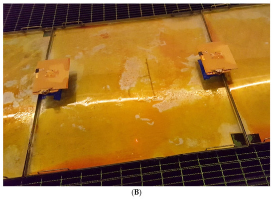
Figure A1.
(A) Photo of one set of glass slide samplers that collected spray droplet deposition; (B) Photo of square trays and the fluorescein dye they collected following one of the runs.
Table A3.
Calculation of mean wind direction angles across 60 s of data via intermediary conversion to cartesian coordinates. Calculations were completed in R software.
Table A3.
Calculation of mean wind direction angles across 60 s of data via intermediary conversion to cartesian coordinates. Calculations were completed in R software.
| Conversion Step | Formula |
|---|---|
| Convert degrees to radians | Used R package NISTunits [42] |
| Convert radians to X dimension, and take mean of all measurements within 60 s | |
| Convert radians to Y dimension, and take mean of all measurements within 60 s | |
| Back-calculate average angle; returns values between -pi radians to pi radians | |
| Convert radians to degrees | Used R package NISTunits [42] |
| Convert scale from −180 to 180 to 0 to 360 | If degree value was negative, add 360 |
| Convert angle from meteorological convention to math convention | Take reflection of angle over the non-tunnel-width axis |
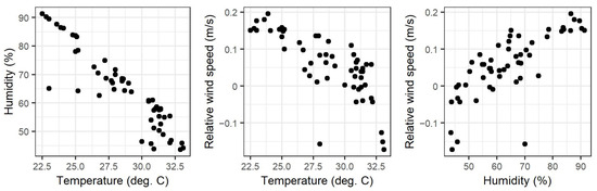
Figure A2.
Correlations among the three meteorological variables, in which each point is the mean value measured during a wind tunnel test using the handheld velocity meter.
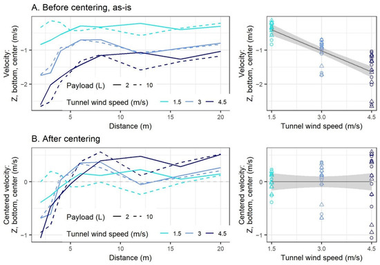
Figure A3.
Example of centering of 3D anemometer measurements within nominal wind speed and payload to prevent multicollinearity in the regression. The example shown is of the variable at the Z dimension, at the bottom height, along the center of the tunnel; all 3D anemometer variables were centered in this way prior to statistical testing. Therefore, these centered variables served to explain differences among distances within runs, rather than differences among runs. Top: as-is, demonstrating correlation; bottom: centered to their means, no longer correlated. Centered variable = measured anemometer wind speed–mean anemometer wind speed among all distances at X m/s and Y L, where X was 1.5, 3.0, or 4.5 m/s and Y was 2 or 10 L. Solid lines and circles represent a 2-L payload, and dotted lines and triangles represent a 10-L payload.
Figure A4.
Graph showing the single excluded outlier, circled at the farthest distance (20 m). Its value was 0.11 ng/cm2, 89 times smaller than the next-highest value of 9.92 ng/cm2 among the remainder of the downwind points. It occurred with the Lechler nozzle, 1.5 m/s, 10 L payload, first replicate. No documentation existed to explain its unusually low mass.
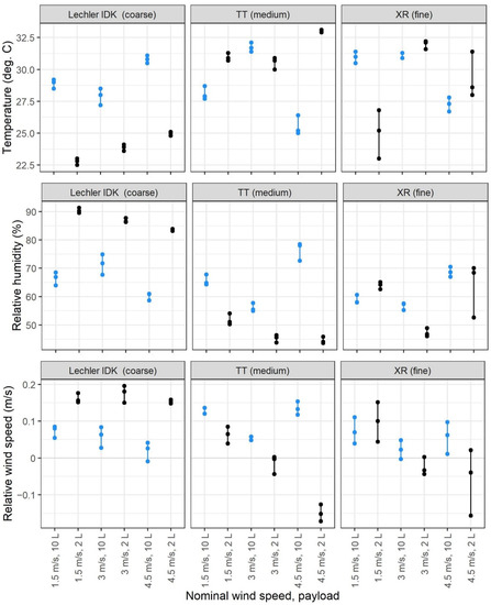
Figure A5.
Meteorological mean values of each wind tunnel run, labeled by nozzle in columns and by wind speed and initial tank payload on the X axis. Each point is a replicate. Black: 2-L payload; blue: 10-L payload.
Table A4.
Equations written from Table 3 for the different nozzles, wind speeds, and payloads. Font colors help associate terms to their variables. Since the regression was built to explain ln(ng/cm2), the full right side of the equation is exponentiated with base e. Most terms are dummy variables of 1 or 0; as such, coefficients are multiplied by 1 (therefore 1 is not shown) or 0 (entire term drops out). The two covariates were only included to reduce noise and enable more precise estimates of the three study design variables of interest; therefore, their means are only included here. The meteorological interaction variable’s mean was 0.181. The 3D anemometer variable’s mean was 0 m/s, so its term fully drops out and is not shown.
| Nozzle | Wind Speed (m/s) | Payload (L) | Equation to Estimate: Mean Deposition in ng/cm2 = |
|---|---|---|---|
| Lechler IDK (coarse) | 1.5 | 2 | |
| 10 | |||
| 3 | 2 | ||
| 10 | |||
| 4.5 | 2 | ||
| 10 | |||
| TT (medium) | 1.5 | 2 | |
| 10 | |||
| 3 | 2 | ||
| 10 | |||
| 4.5 | 2 | ||
| 10 | |||
| XR (fine) | 1.5 | 2 | |
| 10 | |||
| 3 | 2 | ||
| 10 | |||
| 4.5 | 2 | ||
| 10 |
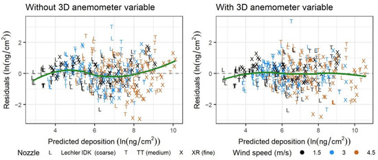
Figure A6.
Residual plot without (left) and with (right) the 3D anemometer variable in the downwind regression. With the variable, the green center LOESS curve is more linear, and the points are more vertically compact around the 0-residual line.
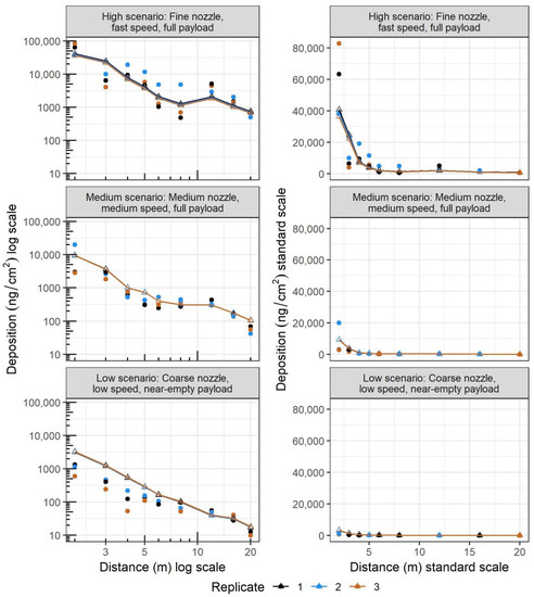
Figure A7.
Actual measurements (circle points) and predictions (triangles with lines) among the three replicates (colors) in each of these three examples. The high, medium, and low scenarios were chosen to demonstrate the range of depositions in this experiment. Left: axes on log scale as statistically analyzed; right: standard scale. Replicates varied by meteorological conditions. The prediction lines are not straight on the log scale but bend with distance especially in the high and medium scenarios, due to the Z-dimension 3D anemometer variable.
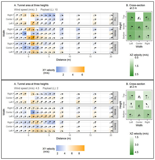
Figure A8.
All remaining combinations of Figure 9. Wind direction and velocity measured using the 3D anemometer. The plots are arranged in the following order according to nominal wind speed and initial payload: 1.5 m/s and 2 L (topmost), 1.5 m/s and 10 L (second), 3 m/s and 2 L (third), 3 m/s and 10 L (fourth), and 4.5 m/s and 2 L (fifth). (A): On a plane parallel to the floor, arrows show direction while cell values and color show the combined X- and Y-dimension velocities. (B): Along the cross-section of the tunnel at a distance of 2 m from the UAV, color shows the combined X- and Z-dimension velocities.
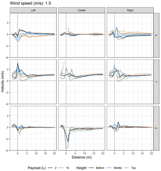
Figure A9.
Wind speeds in three dimensions (rows labeled on right), at three tunnel widths (columns labeled across the top), and at three heights (colors). Figure spans three pages, with one nominal tunnel wind speed per page as labeled on top. Lines break where data are missing, near the UAV itself.
References
- United States Environmental Protection Agency (US EPA). Session 4: UAVs. In Proceedings of the Pesticide Program Dialogue Committee, Arlington, VA, USA, 8–9 May 2019; Available online: https://www.epa.gov/pesticide-advisory-committees-and-regulatory-partners/pesticide-program-dialogue-committee-1 (accessed on 10 April 2020).
- Carvalho, F.; Chechetto, R.; Mota, A.; Antuniassi, U. Challenges of Aircraft and Drone Spray Applications. Outlooks Pest. Manag. 2020, 31, 83–88. [Google Scholar] [CrossRef]
- Crop Life International. Drones Manual—Stewardship Guidance for Use of Unmanned Aerial Vehicles (Uavs) for Application of Crop. Protection Products; Crop Life International: Brussel, Belgium, 2020. [Google Scholar]
- US EPA. Emerging Application Technologies. Available online: https://www.epa.gov/sites/production/files/2018-11/documents/session-3-emerging-application-technologies-l-trossbach.pdf (accessed on 10 April 2020).
- Teske, M.E.; Bird, S.L.; Esterly, D.M.; Ray, S.L.; Perry, S.G. A User’s Guide for Agdrift 2.0.07: A Tiered Approach for the Assessment of Spray Drift of Pesticides. 2003. Available online: https://www.epa.gov/pesticide-science-and-assessing-pesticide-risks/models-pesticide-risk-assessment#AgDrift (accessed on 1 December 2021).
- US EPA. Agdrift®—A Tiered Approach for the Assessment of Spray Drift of Pesticides, 2.1.1; United States Environmental Protection Agency: Washington, DC, USA, 2003. [Google Scholar]
- Ahmad, F.; Qiu, B.; Dong, X.; Ma, J.; Huang, X.; Ahmed, S.; Ali Chandio, F. Effect of Operational Parameters of UAV Sprayer on Spray Deposition Pattern in Target and Off-Target Zones During Outer Field Weed Control Application. Comput. Electr. Agric. 2020, 172, 105350. [Google Scholar] [CrossRef]
- Brown, C.R.; Giles, D.K. Measurement of Pesticide Drift from Unmanned Aerial Vehicle Application to a Vineyard. Trans. ASABE 2018, 61, 1539–1546. [Google Scholar] [CrossRef]
- Chen, S.; Lan, Y.; Zhou, Z.; Ouyang, F.; Wang, G.; Huang, X.; Deng, X.; Cheng, S. Effect of Droplet Size Parameters on Droplet Deposition and Drift of Aerial Spraying by Using Plant Protection UAV. Agronomy 2020, 10, 195. [Google Scholar] [CrossRef]
- Hunter, J.E.; Gannon, T.W.; Richardson, R.J.; Yelverton, F.H.; Leon, R.G. Coverage and Drift Potential Associated with Nozzle and Speed Selection for Herbicide Applications Using an Unmanned Aerial Sprayer. Weed Technol. 2020, 34, 235–240. [Google Scholar] [CrossRef]
- Li, L.; Liu, Y.; He, X.; Song, J.; Zeng, A.; Zhichong, W.; Tian, L. Assessment of Spray Deposition and Losses in the Apple Orchard from Agricultural Unmanned Aerial Vehicle in China. In Proceedings of the 2018 ASABE Annual International Meeting, St. Joseph, MI, USA, 29 July–1 August 2018; p. 1. [Google Scholar]
- Lou, Z.; Xin, F.; Han, X.; Lan, Y.; Duan, T.; Fu, W. Effect of Unmanned Aerial Vehicle Flight Height on Droplet Distribution, Drift and Control of Cotton Aphids and Spider Mites. Agronomy 2018, 8, 187. [Google Scholar] [CrossRef]
- Wang, C.; He, X.; Wang, X.; Wang, Z.; Wang, S.; Li, L.; Bonds, J.; Herbst, A. Testing Method and Distribution Characteristics of Spatial Pesticide Spraying Deposition Quality Balance for Unmanned Aerial Vehicle. Int. J. Agric. Biol. Eng. 2018, 11, 18–26. [Google Scholar] [CrossRef]
- Wang, J.; Lan, Y.B.; Zhang, H.; Zhang, Y.L.; Wen, S.; Yao, W.; Deng, J. Drift and Deposition of Pesticide Applied by UAV on Pineapple Plants under Different Meteorological Conditions. Int. J. Agric. Biol. Eng. 2018, 11, 5–12. [Google Scholar] [CrossRef]
- Wang, X.; He, X.; Song, J.; Wang, Z.; Wang, C.; Wang, S.; Wu, R.; Meng, Y. Drift Potential of UAV with Adjuvants in Aerial Applications. Int. J. Agric. Biol. Eng. 2018, 11, 54–58. [Google Scholar] [CrossRef]
- Wang, X.; He, X.; Wang, C.; Wang, Z.; Li, L.; Wang, S.; Bonds, J.; Herbst, A.; Wang, Z. Spray Drift Characteristics of Fuel Powered Single-Rotor UAV for Plant Protection. Trans. Chin. Soc. Agric. Eng. 2017, 33, 117–123. [Google Scholar] [CrossRef]
- Xue, X.; Kang, T.; Weicai, Q.; Yubin, L.; Huihui, Z. Drift and Deposition of Ultra-Low Altitude and Low Volume Application in Paddy Field. Int. J. Agric. Biol. Eng. 2014, 7, 23–28. [Google Scholar] [CrossRef]
- Martin, D.E.; Woldt, W.E.; Latheef, M.A. Effect of Application Height and Ground Speed on Spray Pattern and Droplet Spectra from Remotely Piloted Aerial Application Systems. Drones 2019, 3, 83. [Google Scholar] [CrossRef]
- Wang, C.; Zeng, A.; He, X.; Song, J.; Herbst, A.; Gao, W. Spray Drift Characteristics Test of Unmanned Aerial Vehicle Spray Unit under Wind Tunnel Conditions. Int. J. Agric. Biol. Eng. 2020, 13, 13–21. [Google Scholar] [CrossRef]
- Wang, L.; Chen, D.; Yao, Z.; Ni, X.; Wang, S. Research on the Prediction Model and Its Influencing Factors of Droplet Deposition Area in the Wind Tunnel Environment Based on UAV Spraying. IFAC-Pap. 2018, 51, 274–279. [Google Scholar] [CrossRef]
- Yang, F.; Xue, X.; Cai, C.; Sun, Z.; Zhou, Q. Numerical Simulation and Analysis on Spray Drift Movement of Multirotor Plant Protection Unmanned Aerial Vehicle. Energies 2018, 11, 2399. [Google Scholar] [CrossRef]
- Zhan, Y.; Chen, P.; Xu, W.; Chen, S.; Han, Y.; Lan, Y.; Wang, G. Influence of the Downwash Airflow Distribution Characteristics of a Plant Protection UAV on Spray Deposit Distribution. Biosyst. Eng. 2022, 216, 32–45. [Google Scholar] [CrossRef]
- Berner, B.; Chojnacki, J. Use of Drones in Crop Protection. In Proceedings of the Farm Machinery and Processes Management in Sustainable Agriculture, IX International Scientific Symposium, Lublin, Poland, 22–24 November 2017; pp. 46–51. [Google Scholar]
- Lv, M.; Xiao, S.; Tang, Y.; He, Y. Influence of UAV Flight Speed on Droplet Deposition Characteristics with the Application of Infrared Thermal Imaging. Int. J. Agric. Biol. Eng. 2019, 12, 10–17. [Google Scholar] [CrossRef]
- Tang, Y.; Hou, C.J.; Luo, S.M.; Lin, J.T.; Yang, Z.; Huang, W.F. Effects of Operation Height and Tree Shape on Droplet Deposition in Citrus Trees Using an Unmanned Aerial Vehicle. Comput. Electr. Agric. 2018, 148, 1–7. [Google Scholar] [CrossRef]
- Zhu, H.; Jiang, Y.; Li, H.; Li, J.; Zhang, H. Effects of Application Parameters on Spray Characteristics of Multi-Rotor UAV. Int. J. Precis. Agric. Aviat. 2019, 2, 18–25. [Google Scholar] [CrossRef]
- Chen, Y.; Hou, C.; Tang, Y.; Zhuang, J.; Lin, J.; Luo, S. An Effective Spray Drift-Reducing Method for a Plant-Protection Unmanned Aerial Vehicle. Int. J. Agric. Biol. Eng. 2019, 12, 14–20. [Google Scholar] [CrossRef]
- ISO 25358; Crop Protection Equipment—Droplet-Size Spectra from Atomizers—Measurement and Classification. International Organization for Standardization: Geneva, Switzerland, 2018; Volume 7.
- R Core Team. R: A Language and Environment for Statistical Computing, 4.2.0; R Foundation for Statistical Computing: Vienna, Austria, 2022. [Google Scholar]
- Wickham, H. Ggplot2 (V3.3.6): Elegant Graphics for Data Analysis; Springer: New York, NY, USA, 2016. [Google Scholar]
- Fox, J.; Weisberg, S. An R Companion to Applied Regression, 3rd ed.; Companion to Applied Regression (CAR) package v.3.0.13; Sage: Los Angeles, CA, USA, 2019. [Google Scholar]
- Hewitt, A.J.; Johnson, D.R.; Fish, J.D.; Hermansky, C.G.; Valcore, D.L. Development of the Spray Drift Task Force Database for Aerial Applications. Environ. Toxicol. Chem. 2002, 21, 648–658. [Google Scholar] [CrossRef] [PubMed]
- Teske, M.E.; Wachspress, D.A.; Thistle, H.W. Prediction of Aerial Spray Release from Uavs. Trans. ASABE 2018, 61, 909–918. [Google Scholar] [CrossRef]
- Chen, H.; Lan, Y.; Fritz, B.K.; Hoffmann, W.C.; Liu, S. Review of Agricultural Spraying Technologies for Plant Protection Using Unmanned Aerial Vehicle (UAV). Int. J. Agric. Biol. Eng. 2021, 14, 38–49. [Google Scholar] [CrossRef]
- Zhang, H.C.; Zheng, J.; Zhou, H.; Dorr, G.J. Droplet Deposition Distribution and Off-Target Drift During Pesticide Spraying Operation. Nongye Jixie Xuebao Trans. Chin. Soc. Agric. Mach. 2017, 48, 114–122. [Google Scholar] [CrossRef]
- US EPA. Annual Spray Drift Review. Available online: https://archive.epa.gov/scipoly/sap/meetings/web/html/spraydrift.html (accessed on 4 May 2022).
- Wang, G.; Han, Y.; Li, X.; Andaloro, J.; Chen, P.; Hoffmann, W.C.; Han, X.; Chen, S.; Lan, Y. Field Evaluation of Spray Drift and Environmental Impact Using an Agricultural Unmanned Aerial Vehicle (UAV) Sprayer. Sci. Total Environ. 2020, 737, 139793. [Google Scholar] [CrossRef] [PubMed]
- Herbst, A.; Bonds, J.; Wang, Z.; Zeng, A.; He, X.; Goff, P. The Influence of Unmanned Agriculturalaircraft System Design on Spray Drift. J. Für Kult. 2020, 72, 1–11. [Google Scholar] [CrossRef]
- Ferguson, J.C.; Chechetto, R.G.; O’Donnell, C.C.; Dorr, G.J.; Moore, J.H.; Baker, G.J.; Powis, K.J.; Hewitt, A.J. Determining the Drift Potential of Venturi Nozzles Compared with Standard Nozzles across Three Insecticide Spray Solutions in a Wind Tunnel. Pest Manag. Sci. 2016, 72, 1460–1466. [Google Scholar] [CrossRef] [PubMed]
- Liu, Q.; Chen, S.; Wang, G.; Lan, Y. Drift Evaluation of a Quadrotor Unmanned Aerial Vehicle (UAV) Sprayer: Effect of Liquid Pressure and Wind Speed on Drift Potential Based on Wind Tunnel Test. Appl. Sci. 2021, 11, 7258. [Google Scholar] [CrossRef]
- International Organization for Standardization. Equipment for Crop Protection—Methods for the Laboratory Measurement of Spray Drift—Wind Tunnels. ISO 22856; International Organization for Standardization: Geneva, Switzerland, 2008. [Google Scholar]
- Gama, J. NISTunits (v1.0.1). Fundamental Physical Constants and Unit Conversions from NIST; 2016. Available online: https://CRAN.R-project.org/package=NISTunits (accessed on 2 April 2022).
Publisher’s Note: MDPI stays neutral with regard to jurisdictional claims in published maps and institutional affiliations. |
© 2022 by the authors. Licensee MDPI, Basel, Switzerland. This article is an open access article distributed under the terms and conditions of the Creative Commons Attribution (CC BY) license (https://creativecommons.org/licenses/by/4.0/).