A Cascaded and Adaptive Visual Predictive Control Approach for Real-Time Dynamic Visual Servoing

Abstract

In the past two decades, Unmanned Aerial Vehicles (UAVs) have gained attention in applications such as industrial inspection, search and rescue, mapping, and environment monitoring. However, the autonomous navigation capability of UAVs is aggravated in GPS-deprived areas such as indoors. As a result, vision-based control and guidance methods are sought. In this paper, a vision-based target-tracking problem is formulated in the form of a cascaded adaptive nonlinear Model Predictive Control (MPC) strategy. The proposed algorithm takes the kinematics/dynamics of the system, as well as physical and image constraints into consideration. An Extended Kalman Filter (EKF) is designed to estimate uncertain and/or time-varying parameters of the model. The control space is first divided into low and high levels, and then, they are parameterised via orthonormal basis network functions, which makes the optimisation- based control scheme computationally less expensive, therefore suitable for real-time implementation. A 2-DoF model helicopter, with a coupled nonlinear pitch/yaw dynamics, equipped with a front-looking monocular camera, was utilised for hypothesis testing and evaluation via experiments. Simulated and experimental results show that the proposed method allows the model helicopter to servo toward the target efficiently in real-time while taking kinematic and dynamic constraints into account. The simulation and experimental results are in good agreement and promising.

1. Introduction

In recent years, rapid development in UAV technology has led to evolutionary application domains. Unmanned Aerial Vehicles (UAVs) are being employed in applications related to agriculture, military, search and rescue, aerial photography, health care, and environment monitoring. To enable the autonomous operation of UAVs, the research community focuses on enhancing kinematic/dynamic modelling, real-time motion planning, guidance, navigation, and trajectory control. Recently, there has been an increased focus on improving the control performance and robust manoeuvrability of UAVs. In the past two decades, and due to an exponential increase in indoor applications, UAVs equipped with camera vision have emerged. This has shifted the research community’s focus towards the design and development of fast, yet robust, vision-based flight control strategies. Academic research on visual navigation and path planning for UAVs has seen a quantum leap. Further developments of their algorithmic foundation in the realm of vision-based control of UAVs have gained significant attention.

As part of the vision-based robot control method, called Visual Servoing (VS), visual sensor data are used to guide the motion of a robot. VS systems use images taken by a camera to measure the error between the robot’s current and desired poses. In other words, images taken by the camera provide feedback to the servo motion control of the robot. In terms of control architecture and error function definitions, VS methods can be classified as (1) Image-Based Visual Servoing (IBVS), (2) Position-Based Visual Servoing (PBVS), and (3) Hybrid Visual Servoing (HVS) [1,2]. The PBVS methods provide robot trajectory paths that are feasible in a 3D space. However, pose estimation, as a critical element of PBVS, can be susceptible to camera calibration errors. Furthermore, the target model must be known beforehand. IBVS, on the other hand, relies on the 2D camera images for the 3D robot trajectory; thus, the trajectories might not be physically feasible in the 3D action space. Moreover, the IBVS system might be subject to the singularity of the Jacobian problem [1]. Hybrid VS (HVS) is a method that combines IBVS and PBVS and addresses some of the shortcomings mentioned above [3].

On a separate line, the development of Model Predictive Control (MPC) has provided the essential infrastructure to formulate VS as a constrained optimisation problem. The main objective of Visual Predictive Controllers (VPCs) is to provide a systematic framework to accomplish VS problems in a mathematically optimal fashion while taking the inputs, states, and task constraints into account [4]. In most of the proposed VPC approaches, constraints due to the camera’s Field of View (FoV), the kinematics of the robot, and sensor/inputs saturation are considered. Despite this, no systematic strategy has been provided in the above-mentioned literature to deal with system/measurement uncertainties.

VPC systems are prone to uncertainties due to a variety of factors including imperfect system models, measurement noises, and exogenous disturbances. Some uncertainties in the VS system may have a parametric/deterministic nature (e.g., kinematics error in the robot model or calibration error in the focal length of the camera). Adaptive VS methods have been proposed to compensate the deterministic/parametric uncertainties in VS [5,6]. For example, an adaptive camera calibration technique was proposed in [7] to solve the problem of underwater camera calibration in complex underwater environments affected by changing optical conditions. Many of the adaptive VS techniques rely on the application of parameter estimation methods such as Extended Kalman Filters (EKFs) and Unscented Kalman Filters (UKFs). Apart from the parametric uncertainties, some system uncertainties involved in the VS task might exhibit stochastic behaviour (e.g., noisy feature detection algorithms). In the presence of random uncertainties, Robust Visual Servoing (RVS) techniques have been explored as a method for improving the performance of VS tasks. The main objectives of RVS are to improve the accuracy and constraint compliance [8] while maintaining stability [9]. Typically, robust VPC methods make use of a bounded deterministic uncertainty model in order to take worst-case uncertainty realisations into account. Despite that robust VPC techniques provide a robust, constraint-compliant solution to system uncertainties, their performance is unnecessarily conservative. In fact, robust VPC ignores the probability-based nature of system uncertainties. To exploit the probability of system uncertainties, Stochastic Visual Predictive Control (SVPC) approaches have been developed [10]. In contrast to robust VPC, which takes the worst-case scenario of uncertainty realisations into account, SVPC algorithms consider the chances of the system encountering those uncertainties. Accordingly, SVPC provides superior control over RVPC in terms of performance and constraint handling. However, RVPC and SVPC method formulations both yield computationally intensive problems, which need to be handled in real-time.

The formulation of the above-mentioned predictive visual servoing problems typically yield a constrained nonlinear optimisation problem to be solved over a finite prediction horizon. Due to the computational complexity of constrained nonlinear optimisation problems, several methods have been suggested by researchers for reducing the time required for computation and making the VPC algorithms more suitable for real-time applications. For example, gain scheduling VPC involves identifying local linear time-invariant state-space models around a family of operating points, designing corresponding linear-model-based predictive controllers, and selecting a scheduling variable suitable to govern the switching process [11]. The other approach proposed in the literature is linearisation through the system Jacobian, where the system model is linearised successively in the proximity of each operation point in each time step [12]. Furthermore, predictive feedback linearisation methods have been proposed to reduce the computational complexity of real-time implementation [13].

The computational complexity of VPC approaches also increases with the size of the control and prediction horizons. In particular, this complication is aggravated when the system dynamics and dynamic constraints are considered in the system model. As a consequence, this problem limits the applicability of VPC to systems with slow dynamics, where it is possible to update control policies frequently enough to maintain stability. A number of approaches have been suggested in the literature to reduce the computational expense of VPC and MPC in general. Parameterising the control policies via orthonormal basis functions has been introduced as a viable solution. The utilisation of these network functions in the MPC formulation would reduce the number of parameters to optimise without compromising the accuracy of the results. The effect of network parameterisation using B-spline functions on decision variables was studied in [14]. Similarly, in [15], Laguerrenetwork functions and in [16] Kautz orthonormal basis function were explored to effectively reduce the computational expense of the MPC in real-time applications.

Cascaded control architectures have also been proposed as a means to further reduce the complexity of dynamic VPC and improve its real-time applicability. As a result of the modular design of the cascaded control architecture, the low- and high-level controllers can be tuned separately. This also enables the system designers to set high- and low-level controllers to run at different sampling speeds. Moreover, the fault detection, diagnosis, and tolerance procedures of the system can be performed more systematically. A two-tier nonlinear predictive visual servoing approach, with applications in vision-based control of UAVs, was presented in [17]. The results reported the simulated control of the UAV, while successfully handling physical and image constraints.

This paper contributes by proposing a cascaded adaptive predictive control approach to conduct a dynamic visual servoing task on a UAV platform in an energy-optimal fashion, while considering kinematics and/or dynamics, image, and actuator constraints. Additionally, a parameter estimator based on the Extended Kalman Filter (EKF) was integrated into the feedback control loop in order to adjust the predictive control strategy on the fly in response to model uncertainties and/or dynamic changes in the system’s physical parameters. Moreover, an orthonormal-network-function-based control input approximation method was developed, which enables real-time experimentation and validation. To the authors’ best knowledge, this paper is the first study in the field of visual servoing that incorporates the dynamics of the motion platform in an adaptive manner while providing a predictive, but computationally efficient solution that increases real-time implementation feasibility. The proposed control strategy was tested via simulations and then implemented on an experimental setup consisting of a helicopter model with two degrees of freedom.

The rest of this article is structured as follows. In Section 2, the general formulation of cascaded VPC-MPC is presented. The kinematic/dynamic models of the test bench are explained briefly in Section 2.1, followed by the formulation for the vision-based control strategy and the image processing algorithm for feature extraction. Furthermore, a detailed description of the controller’s architecture is covered in Section 2.1. The experimental setup is explained in Section 3. In Section 4, the simulation and experimental results are provided. Finally, conclusions and future work can be found in Section 5.

2. Problem Formulation

In this paper, a two-stage controller under a VPC paradigm is proposed. The goal of the proposed two-stage controller is to overcome the shortcomings of existing VPC approaches in real-time applications. Unlike the traditional VPC approaches, which mainly consider the kinematics of the robotic platform, the cascaded design allows taking the dynamics of the robot, as well as dynamic constraints into account. This control approach optimises an objective function, which is comprised of energy expenditure within a finite time window named the prediction horizon by computing optimal manipulated variables. The dynamics of the locomotion unit in addition to the constraints of the motion, as well as sensor constraints such as the Field of View (FOV) are taken into consideration. The objective of the predictive control approach is to minimise the error between the feature and target points while minimising the energy consumption in the locomotion unit. The balance between minimisation of the robotic platform’s motion and its agility of response to the error in the image is achieved through tuning the coefficients of a quadratic performance index under the MPC formulation. Furthermore, control space parameterisation via orthonormal Laguerre functions decreases the computational load, therefore making the control scheme suitable for real-time applications. The state-space models of the robot and the camera are used to predict the behaviour and states of the system. The discrete state-space model of the robot and the camera can be represented as a general successively linearised model:

$$\left\{\begin{array}{c}{\chi }_{k+1}=A_k{\chi }_k+B_k{u}_k\hfill \\ {\gamma }_k=C_k{\chi }_k+D_k{u}_k,\hfill \end{array}\right.$$

(1)

Matrices $A_k\in {\mathbb{R}}^{n\times n}$, $B_k\in {\mathbb{R}}^{n\times p}$, $C_k\in {\mathbb{R}}^{q\times n}$, and $D_k\in {\mathbb{R}}^{q\times p}$ are the coefficients of the general state-space representation of the discretised dynamic system obtained through successive linearisation of the nonlinear process and measurement model of the system with p inputs, q outputs, and n state variables, where ${\chi }_k\in {\mathbb{R}}^n$, ${\gamma }_k\in {\mathbb{R}}^q$, and $u_k\in {\mathbb{R}}^m$ denote vectors of states and the outputs and inputs of the system, respectively. One can define $\Delta {\chi }_{k+1}={\chi }_{k+1}-{\chi }_k$ and $\Delta u_k=u_{k+1}-u_k$ as incremental variables and obtain the incremental state-space model:

$$\begin{array}{c}\hfill \Delta {\chi }_{k+1}=A_k\Delta {\chi }_k+B_k\Delta u_k.\end{array}$$

(2)

This representation will facilitate the implementation of the Linear-Parameter-Varying (LPV)-based MPC of nonlinear systems through successive linearisation. By the concatenation of the the incremental states and output vector, the augmented state vector can be defined as: $x_k={[\Delta {\chi }_k{\gamma }_k]}^{⊺}$. Finally, the resulting augmented system model with the embedded integrator is given as

$$\left\{\begin{array}{c}\stackrel{x_{k+1}}{\overbrace{\left[\begin{array}{c}\Delta {\chi }_{k+1}\\ {\gamma }_{k+1}\end{array}\right]}}=\stackrel{A}{\overbrace{\left[\begin{array}{cc}{A}_k& \mathbf{O}\\ C_k{A}_k& 1\end{array}\right]}}\stackrel{x_k}{\overbrace{\left[\begin{array}{c}\Delta {\chi }_k\\ {\gamma }_k\end{array}\right]}}+\stackrel{B}{\overbrace{\left[\begin{array}{c}{B}_k\\ C_k{B}_k\end{array}\right]}}\Delta u_k\hfill \\ y_k=\stackrel{C}{\overbrace{\left[\begin{array}{cc}\mathbf{O}& 1\end{array}\right]}}\left[\begin{array}{c}\Delta {\chi }_k\\ {\gamma }_k\end{array}\right],\hfill \end{array}\right.$$

(3)

where $\mathbf{O}={\left[\begin{array}{ccc}0& \dots & 0\end{array}\right]}_{1\times n}$. In the MPC/VPC framework, the quadratic performance index, based on augmented states, can be defined as

$$J(x_k,\Delta u_k,k)=\sum _{i=1}^{N_p}{x}_{k+i|k}^{⊺}Q{x}_{k+i|k}+\sum _{i=1}^{N_c-1}\Delta u_{k+j|k}^{⊺}R\Delta u_{k+j|k},$$

(4)

where $N_p$ is the prediction horizon, $N_c$ is the control horizon, and Q and R are weighting matrices. In each control sequence, the optimal control policy $\Delta U$ can be calculated based on the results of the performance index optimisation. The performance index optimisation problem can be solved subject to system dynamics and constraints over the prediction horizon. The idea proposed in [18], which results in the reduced number of optimisation parameters, hence improving the real-time implementation feasibility of MPC, is to approximate the following control input sequence with discrete polynomials:

$$\begin{array}{c}\hfill \Delta U={[\Delta u_k^{⊺},\Delta u_{k+1}^{⊺},\dots ,\Delta u_{k+N_p-1}^{⊺}]}^{⊺},\end{array}$$

(5)

and in this context, Laguerre functions yield themselves as good candidates for parametrising the decision variable vector due to their orthonormal property and recursive construction identity. Laguerre polynomials can be defined in the z-domain as follows:

$$\begin{array}{c}\hfill L_m\left(z\right)=\sqrt{1-{\alpha }^2}\frac{{(z^{-1}-\alpha )}^{m-1}}{{(1-\alpha z^{-1})}^m};0\le \alpha <1,m\in \mathbb{N},\end{array}$$

(6)

where m denotes the order of the Laguerre functions and $\alpha$ represents the single parameter describing the functions. Letting $l_k$ denote the inverse z-transform of $L(z,\alpha )$ and using Laguerre functions, this design framework approach approximates $\Delta u_{k+i}$ via the following method:

$$\Delta u_{k+i}=L{\left(i\right)}^{⊺}\eta ,$$

(7)

where $L{\left(i\right)}^{⊺}={[l_1\left(i\right)l_2\left(i\right),\dots l_N\left(i\right)]}^{⊺}$, $1\le i\le N_p$, $\eta ={[{\eta }_1^{⊺}{\eta }_2^{⊺}\dots {\eta }_N^{⊺}]}^{⊺}$, and N is the number of basis functions used for approximation. Furthermore, owing to the recursive nature of Laguerre functions, $L(j+1)$ can be calculated recursively:

$$L(j+1)=A_{l}L\left(j\right)$$

(8)

where $L\left(0\right)=\sqrt{\beta }[1-\alpha {\alpha }^2\dots {(-1)}^{N-1}{\alpha }^{N-1}]$, $\beta =(1-{\alpha }^2),0\le \alpha <1$. Accordingly, given $\alpha$ as the only scalar design parameter of Laguerre polynomials, N and $N_p$, one can determine $A_l$ [19]:

$$A_l={\left[\begin{array}{cccc}\alpha & 0& \dots & 0\\ \beta & \alpha & \dots & 0\\ -\alpha \beta & \beta & \dots & 0\\ ⋮& ⋮& ⋮& ⋮\\ {(-\alpha )}^{N-2}\beta & {(-\alpha )}^{N-3}\beta & \dots & \alpha \end{array}\right]}_{N\times N}$$

(9)

The calculation of $A_l$ completes the recursive definition of Laguerre functions with Equation (8).

Figure 1 shows the control block diagram of the proposed cascaded VPC. In this block diagram, the vector, $u^{*}$, represents the joint velocity of the robot and s represents the detected visual features in the image. Moreover, on the block diagram. the system input, u, denotes the joint velocity of the robotic manipulator. s and $s^{*}$ represent the measured visual features and desired feature pose in the image. Furthermore, $\xi$ and $\widehat{\xi }$ represent the measured pose of the robot and the estimated pose by the EKF, respectively. Furthermore, ${\mathbf{H}}_e^c$ denotes a homogeneous transformation matrix utilised to transform $\xi$ into the position of the camera on the robot. The target pose to be followed by the robot, which is generated by the VPC block, is denoted by ${\xi }^{*}$. The major elements of cascaded VPC are the mathematical model of the plant including the camera and the robotic platform, the cost functions for each control stage, and the optimisation methods. In the proposed scheme, the current state error is defined as the difference between the predicted mean of the states of the system, s, and the desired state vector $s^{*}$.

As shown in the block diagram, the first step is to determine the desired robot velocity trajectory by optimising the visual performance index based on image predictions. The optimisation algorithm takes into account the FOV constraints $I(·)$, to ensure that the feature points will not leave the image during the process and the maximum permissible acceleration of joints, $\ddot{\xi }$. A sequential quadratic optimisation problem is also formed by successively linearising the nonlinear mapping between the motion of the robot and the optical flow of a feature point in the image domain, $\zeta (·)$:

$$\begin{array}{c}\underset{\eta }{\mathrm{minimise}:}\sum _{i=1}^{N_p}{s}_{k+i|k}^{⊺}{Q}_1{s}_{k+i|k}+{\eta }^{⊺}{R}_1\eta \hfill \\ \mathrm{subject}\mathrm{to}:s_{k+1}=\zeta (s_k,{\eta }_k)\hfill \\ I_{min}\le I\left(s_k\right)\le I_{max}\hfill \\ {\ddot{\xi }}_{min}\le \ddot{\xi }\le {\ddot{\xi }}_{max}\hfill \end{array}$$

(10)

The result of the optimisation in Equation (10) is the Laguerre coefficient vector $\eta$, which can be used as described in Equation (7) to approximate $\Delta {\dot{\xi }}^{*}$. An MPC framework with a receding horizon pushes only the first element of the manipulated variable forward, while discarding the rest [19]. The output of the “VPC” block is the vector of the desired joint motion velocities ${\dot{\xi }}^{*}$. An integration of the desired velocity will provide desired joint pose trajectories ${\xi }^{*}$, which are fed to the second-stage controller, “MPC”. In the “MPC”, the goal is to minimise the performance index in Equation (11) and to compute optimal inputs to be applied to the robot joints. The dynamics and constraints of the actuators can be considered at this stage. The performance index optimisation problem becomes

$$\begin{array}{c}\underset{\eta }{\mathrm{minimiz}:}\sum _{i=1}^{N_p}{\xi }_{k+i|k}^{⊺}{Q}_2{\xi }_{k+i|k}+{\eta }^{⊺}{R}_2\eta \hfill \\ \mathrm{subject}\mathrm{to}:{\xi }_{k+1}=\Theta ({\xi }_k,\eta k)\hfill \\ u_{min}\le u\le u_{max}\hfill \\ {\xi }_{min}\le \xi \left(k\right)\le {\xi }_{max}\hfill \end{array}$$

(11)

where $\Theta (·)$ describes the dynamics of the robot. Similar to the previous stage “VPC”, the approximation of the optimal inputs to be applied to the joint actuators are conducted through the Laguerre function. The trajectory control performance was also improved further by using an EKF-based states and parameter estimator. EKF-based methods have been extensively used in the literature for state estimation in the presence of noisy sensor measurements [20]. In more recent applications, the EKF has been successfully utilised for simultaneous state and parameter estimation of nonlinear dynamic systems [21,22,23,24]. For this purpose, the general nonlinear state-space representation of the system is augmented by uncertain parameter vector $\tau$. The EKF’s dynamic model then can be represented by

$$X_{k+1}=\left[\begin{array}{c}{x}_{k+1}\\ {\tau }_{k+1}\end{array}\right]=\left[\begin{array}{c}{f}_1(x_k,u_k,{\tau }_k,k)\\ f_2\left({\tau }_k\right)\end{array}\right]+\left[\begin{array}{c}{\omega }_{k1}\\ {\omega }_{k2}\end{array}\right]$$

(12)

where $f_1$ represents the dynamic model of the nonlinear system, $X={\left[x\tau \right]}^{⊺}$ denotes the new state vector augmented with the uncertain parameter vector, and ${\omega }_{k1}$ denotes zero mean process noise with covariance $\Omega$. The uncertainty associated with the parameters to be estimated is denoted by ${\omega }_{k2}$. Moreover, the convergence rate in the parameter estimation can be tuned through assigning values to ${\omega }_{k2}$. Considering that uncertain parameters have stationary values results in $f_2\left({\tau }_k\right)=0$. The measurements can be formulated as

$$Y_k=h\left(X_k\right)+{\nu }_k$$

(13)

where the measurement noise ${\nu }_k$ is modelled as a zero mean white noise with covariance $\Lambda$. According to the EKF method, the measurement and system dynamics are linearised in the proximity of the estimated state ${\widehat{X}}_k$ by obtaining the Jacobian of the system dynamics:

$$F=\frac{\partial f(X,u,t)}{\partial X}{\mid }_{X=\widehat{X}},H=\frac{\partial h\left(X\right)}{\partial X}{\mid }_{X=\widehat{X}}$$

(14)

The EKF algorithm estimates the augmented state vector in two stages, prediction based on the system model and update based on measurements. In the prediction stage, new state vector $X_{k|k-1}$ is calculated with the dynamic system model. Error covariance ${\Sigma }_{k|k-1}^x$ is also determined through the linear error propagation model:

$$\begin{array}{cc}\hfill & X_{k|k-1}=f(X_{k-1|k-1},u_k)\hfill \\ \hfill & {\Sigma }_{k|k-1}^x=F_k{\Sigma }_{k-1|k}^x{F}_k^{⊺}+{\Omega }_k,\hfill \end{array}$$

(15)

In the update stage, sensor measurements improve the predictions of states and error covariance. The Kalman gain ${\mathcal{K}}_k$ then can be calculated,

$$\begin{array}{cc}\hfill & {\mathcal{K}}_k=\frac{{\Sigma }_{k|k-1}^x{H}_k}{H_k{\Sigma }_{k|k-1}^x{H}_k+{\Lambda }_k}\hfill \\ \hfill & {\hat{X}}_{k|k-1}={\hat{X}}_{k|k-1}+{\mathcal{K}}_k(Y_k-h\left(X_k\right))\hfill \\ \hfill & {\Sigma }_{k|k}^x=(\mathbf{I}-{\mathcal{K}}_k{H}_k){\Sigma }_{k|k-1}^x.\hfill \end{array}$$

(16)

where ${\Sigma }_{k|k}^x$ and ${\widehat{X}}_{k|k-1}$ are the improved error covariance and updated augmented state estimation, respectively [25]. As shown in Figure 1, the EKF is implemented first, to enhance the quality of the measurements gathered through the sensor of the robot and, second, to estimate the uncertain or time-varying parameters of the robot and accordingly revise the system model under the “MPC” block.

2.1. Method Validation Case Study

The selected test bench for evaluating the proposed cascaded predictive visual servoing algorithm consists of a 2-DoF model helicopter from Quanser (https://www.quanser.com (accessed on 1 October 2021)), shown in Figure 2. The model helicopter was mounted on a fixed base. Two brush-type DC motors drive the front and tail propellers. The angular positions along the pitch and yaw axes were measured via high-resolution quadrature encoders. The pitch motion was physically restricted; however, the helicopter is capable of rotating freely along the yaw axis, due to the slip ring mechanism utilised. The derivation of the governing dynamics equations of the helicopter’s motion based on Lagrange’s method can be found in [26]. The dynamics equations are:

$$\begin{array}{cc}\hfill & (J_{eq,p}+m_{heli}{l}_{cm}^2)\ddot{\theta }=K_{pp}{V}_{m,p}+k_{py}{V}_{m,y}-m_{heli}g{l}_{cm}\cos \theta \hfill \\ \hfill & -B_p\dot{\theta }-m_{heli}\sin \theta \cos \theta {\dot{\psi }}^2\hfill \\ \hfill & (J_{eq,y}+m_{heli}{l}_{cm}^2{\cos }^2\theta )\ddot{\psi }=K_{yp}{V}_{m,p}+k_{yy}{V}_{m,y}-B_y\dot{\psi }\hfill \\ \hfill & +2m_{heli}{l}_{cm}\sin \theta \cos \theta \dot{\psi }\dot{\theta }\hfill \end{array}$$

(17)

Figure 2. Quanser 2-DoF model helicopter [27].

Figure 2. Quanser 2-DoF model helicopter [27].

The parameters in Equation (17) are explained in

Table 1. Physical parameters of the Quanser 2-DoF helicopter.

Variable	Value	Unit	Parameter Description
$\theta$	$[-0.706,+0.706]$	$\left(\mathrm{rad}\right)$	Pitch angle
$\psi$	$[-\infty ,+\infty ]$	$\left(\mathrm{rad}\right)$	Yaw angle
g	9.81	(m/s2)	Gravity constant
$m_{heli}$	$1.387$	(kg)	Total moving mass of the helicopter
$l_{cm}$	$0.029$	(m)	Position of centre of mass from pitch axis
$B_p$	$0.015$	(N/V)	Viscous damping of the pitch axis
$B_y$	$0.025$	(N/V)	Viscous damping of the yaw axis
$J_{eq,p}$	$0.034$	(kg m2)	Moment of inertia about pitch pivot
$J_{eq,y}$	$0.039$	(kg m2)	Moment of inertia about yaw pivot
$K_{pp}$	$0.021$	(Nm/V)	Thrust torque coefficient of pitch propeller on pitch angle
$K_{yp}$	$0.003$	(Nm/V)	Thrust torque coefficient of pitch propeller on yaw angle
$K_{yy}$	$0.011$	(Nm/V)	Thrust torque coefficient of yaw propeller on yaw angle
$K_{py}$	$0.001$	(Nm/V)	Thrust torque coefficient of yaw propeller on pitch angle

. $\theta$ and $\psi$, namely the pitch and yaw angular positions, represent two degrees of freedom. The helicopter is capable of hovering around any pitch angle while rotating along the yaw axis. The Centre Of Mass (COM) is located with an offset to the rotation axis, which makes the state-space representation of the system time-varying and state-dependent. In addition, the pitch and yaw motions are dynamically coupled. Each motor applies a counter-torque onto the fuselage due to the gyroscopic effect.

The maximum allowed voltages applied to the pitch and yaw motors are rated as ±24 V and ±15 V, respectively. The blades used in our model helicopter were designed by the manufacturer in a way that they could generate thrust efficiently only when rotating in a certain direction. In general, the propellers in rotary-wing flyers are designed to give only upward lift. For downward force, usually, this is left to gravity. Our model helicopter was not an exception to this. The blades could provide lift efficiently only when turning in a certain direction. The aforementioned blade design would make our model helicopter more energy efficient. Downward motion was achieved by using the passive force due to gravity, after the motors were switched off.

Considering $\xi =[\theta ,\dot{\theta },\psi ,\dot{\psi }]$ as the state vector of the 2-DoF helicopter and $u=[V_{m,p}$, $V_{m,y}]$ as the manipulated variables, the nonlinear coupled dynamics of the helicopter can be represented in the compact form given in Equation (18), where the kinematic constraints and voltage limits applied to the propeller motors are included in the following formulation:

$$\begin{array}{c}{\xi }_{k+1}=\Theta ({\xi }_k,u_k)\\ u_{min}\le u\le u_{max}\\ {\xi }_{min}\le {\xi }_k\le {\xi }_{max}.\end{array}$$

(18)

A 3-megapixel (Logitech C270) webcam [28] with a Complementary Metal–Oxide Semiconductor (CMOS) sensor, capable of streaming video at 30 frames per second with 720 × 1280 resolution, was attached to the tip of the helicopter as a front-looking camera. In the experiments, the camera motion was controlled to track an orange-colour ping-pong ball moving in front of a blue screen (see Figure 3 and Figure 4).

A projection model was developed that captures the mathematical relation between the 3D location of points in the physical space and their 2D pixel coordinates within the captured image. In this work, a perspective projection model (also known as pinhole projection model) was adopted. Further details on this model can be found in [29,30]. According to the pinhole projection model, the mapped position of any arbitrary world point $\Pi ={\left[xyz1\right]}^{⊺}$ in the 2D image domain, ${\Pi }^{\prime }={\left[\alpha \beta 1\right]}^{⊺}$, would depend on two sets of parameters. known as intrinsic and extrinsic. Intrinsic parameters depend on the structural features of the camera such as: the focal length, $\lambda$, the size of pixels on the CMOS sensor array, $\rho$, skewness, $\varpi$,and lens distortion. Furthermore, $u^0$ and $v^0$ represent the principal coordinates of the image. On the other hand, the extrinsic parameters include spatial information such as: the position and orientation of the camera with respect to the world reference frame. Accordingly, the pinhole projection model of the camera can be formulated as

$$\begin{array}{c}{\Pi }^{\prime }=\underset{intrinsic}{\underbrace{\left[\begin{array}{ccc}\lambda /\rho & \varpi & u^0\\ 0& \lambda /\rho & v^0\\ 0& 0& 1\end{array}\right]\left[\begin{array}{cccc}1& 0& 0& 0\\ 0& 1& 0& 0\\ 0& 0& 1& 0\end{array}\right]}}\underset{extrinsic}{\underbrace{{\left[\begin{array}{cc}{R}_{3\times 3}& T_{3\times 1}\\ 0& 1\end{array}\right]}^{-1}}}\Pi \end{array}$$

(19)

Moreover, Equation (19) can be re-written in compact form as ${\Pi }^{\prime }=G{T}_h\Pi$, where matrix G reflects the intrinsic parameters and $T_h$ denotes the homogeneous transformation matrix of projecting camera coordinates with respect to the global reference frame.

Estimating the extrinsic and intrinsic parameters of a camera is a process known as camera calibration [18]. In this work, the camera calibration toolbox of MATLAB was utilised for this purpose [31]. Camera parameters were then used to form the image Jacobian $L_s(s,Z)$, as in Equations (20) and (21), where $s=[u,v]$ denotes the vector coordinate of the projected point feature and Z denotes the depth of the feature point, representing how far the feature point is from the camera’s projection centre (see Figure 3).

For any given velocity of the camera frame $v^c\in {\mathbb{R}}^{6\times 1}$, the optical flow on image features is denoted by $\dot{s}=[{\dot{u}}_1{\dot{v}}_1...{\dot{u}}_k{\dot{v}}_k{]}_{2k\times 1}^{⊺}$, which can be estimated by using the image Jacobian (also known as the interaction matrix) denoted by $L_s(s,Z)\in {\mathbb{R}}^{2k\times 6}$. The interaction matrix described in Equation (20) relates the velocity of $k\in \mathbb{N}$ feature points in the image domain to the camera velocity vector:

$$\dot{s}=L_s(s,Z)v^c$$

(20)

Given a pinhole camera projection model and a single point feature interaction matrix, the image Jacobian, $L_s(s,Z)$, can be written as in Equation (21), where $f^{\prime }=\lambda /\rho$ [32].

$$\begin{array}{c}{L}_s=\left[\begin{array}{cccccc}\frac{-f^{\prime }}{Z}& 0& \frac{u}{Z}& \frac{uv}{f^{\prime }}& -\frac{f^{\prime 2}+u^2}{f^{\prime }}& v\\ 0& \frac{-f^{\prime }}{Z}& \frac{v}{Z}& -\frac{f^{\prime 2}+v^2}{f^{\prime }}& -\frac{uv}{f^{\prime }}& -u\end{array}\right]\end{array}$$

(21)

Furthermore, the velocity of the camera attached to the tip of the helicopter $v^c$ could be related to the angular velocities of the pitch and yaw, $\dot{q}=[\dot{\theta },\dot{\psi }]$, via the helicopter’s Jacobian $J_r$. Finally, the optical flow $\dot{s}$ associated with a point of interest in the image domain could be then formulated in a compact form:

$$\begin{array}{c}{s}_{k+1}=s_k+L_s(s,Z)J_r\left(\xi \right){\dot{q}}_k\\ I_l\le s_k\le I_u\\ s=[\alpha ,\beta ],q=[\theta ,\psi ],\end{array}$$

(22)

where the camera’s Field Of View (FOV) constraints are encapsulated in the I. The Jacobian of the system $J_r$ maps the helicopter’s motion to that in the camera by $v^c=J_r\dot{q}$, where the 2-DoF model helicopter’s Jacobian $J_r$ can be modelled as

$$\begin{array}{c}\hfill J_r(\theta ,\psi )=\left[\begin{array}{cc}-l\sin \theta \cos \psi & -l\cos \psi \sin \theta \\ l\cos \psi \cos \theta & -l\sin \psi \sin \theta \\ 0& l\cos \theta \\ 0& \sin \psi \\ 0& -\cos \theta \\ 1& 0\end{array}\right],\end{array}$$

(23)

where l denotes the distance between the centre of rotation on the helicopter’s stand and the camera’s projection centre. Furthermore, the projection centre of the camera and the centre of rotation of the helicopter are both located on the longitudinal axis of the helicopter, aligned with the pitch axis.

3. Experimental Setup

The 2-DoF model helicopter from Quanser was interfaced to a Windows host computer through a USB Data Acquisition (DAQ) card. The motion of the helicopter was measured through rotary encoders via a slip ring. Control signals were conditioned via a linear power amplifier to drive the pitch/yaw motors.

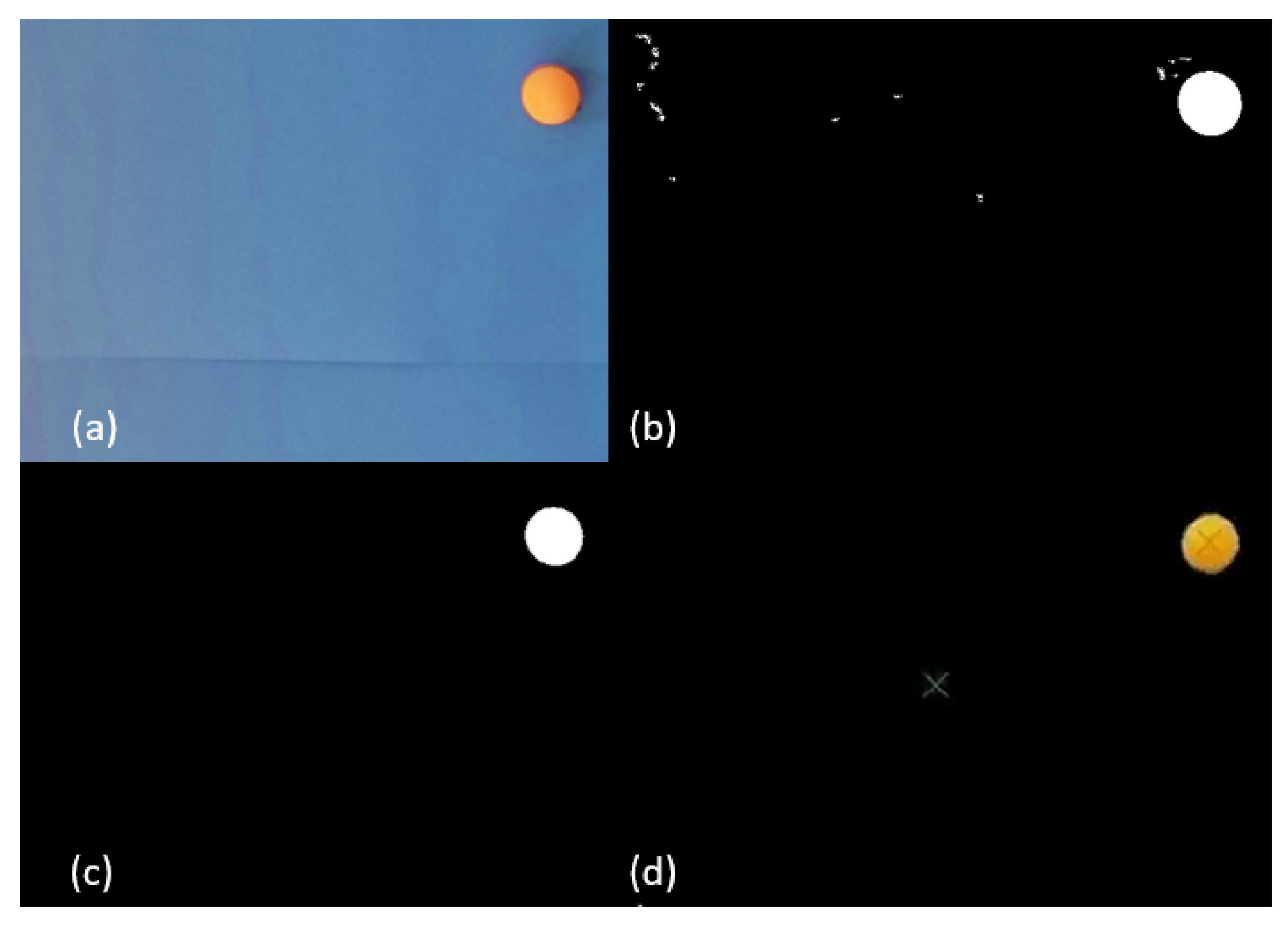
Real-time images, for the visual servoing task, were acquired via a light-weight USB camera (Logitech C270) attached to the tip of the helicopter. A conventional image processing algorithm was implemented to distinguish an orange ping-pong ball from the high-contrast blue background, as shown in Figure 3. The algorithm tracks the centre point of the orange ball in the image. In unstructured and real-world scenarios subject to a cluttered background, the target in the image should be detected using more robust techniques such as those based on deep learning techniques. In this paper, the main focus was on the design of the controller; therefore, a simple blob-centroid-detection algorithm was used for tracking the target. Finding the centroid of the ball was carried out by following simple image processing steps: First, the camera acquires the Red-Green-Blue (RGB) image at a 720 × 1280 pixel resolution. In order to improve the processing rate, the captured image is then down-sampled to 640 × 420 pixels. Second, the down-sampled image is converted to the Hue-Saturation-Value (HSV) space to increase the robustness of the ball-tracking algorithm to the external lighting disturbances. Third, the resultant image is segmented into a binary map by using a colour threshold filter, which differentiates the position of the ball from the rest of the image. Finally, the binary image was used to determine the coordinates of the centroid (see Figure 5). Methods for estimating the depth of target for VS to irregular shapes can be challenging and were extensively studied in [33,34]. However, in this case study, the diameter of the ball in the image can be easily extracted and utilised for the depth estimation purposes.

Furthermore, the accuracy of the algorithm is increased by filtering the noise in the image bitmap. Lastly, the centroid of the ball is reverted to its original colour, and the centre of the image frame is marked, as illustrated in Figure 5.

The proposed control approach and image processing algorithm were implemented in Simulink^®. The camera feed was interfaced to the Simulink model through the Webcam Support extension package [35]. The image processing and feature detection algorithms were developed using the functions and libraries provided in the Computer Vision Toolbox™ [36]. Furthermore, MATLAB functions and scripts were developed for the implementation of the prediction models, control algorithms, and the Quadratic Programming (QP) optimisation routine. The MATLAB functions were then converted into Simulink blocks through the process described in [37] for system integration.

The processing speed of the real-time implementation was accelerated through using Simulink^® Coder^™, which generates C/C++ code and runs it on the operating system as a native application.

4. Simulation and Experimental Results

The effectiveness and validity of the proposed cascaded predictive visual servoing/tracking method was validated via various simulations and experiments. In both the simulations and experiments, the following tests were conducted: An orange ball, attached to a stick, was located within the camera’s FOV. The proposed control algorithm then tries to bring the image of the orange ball to the centre point of the pixel frame. The goal is to align the optical axis of the camera with the centroid of the orange ball, while optimising the performance index and considering the constraints.

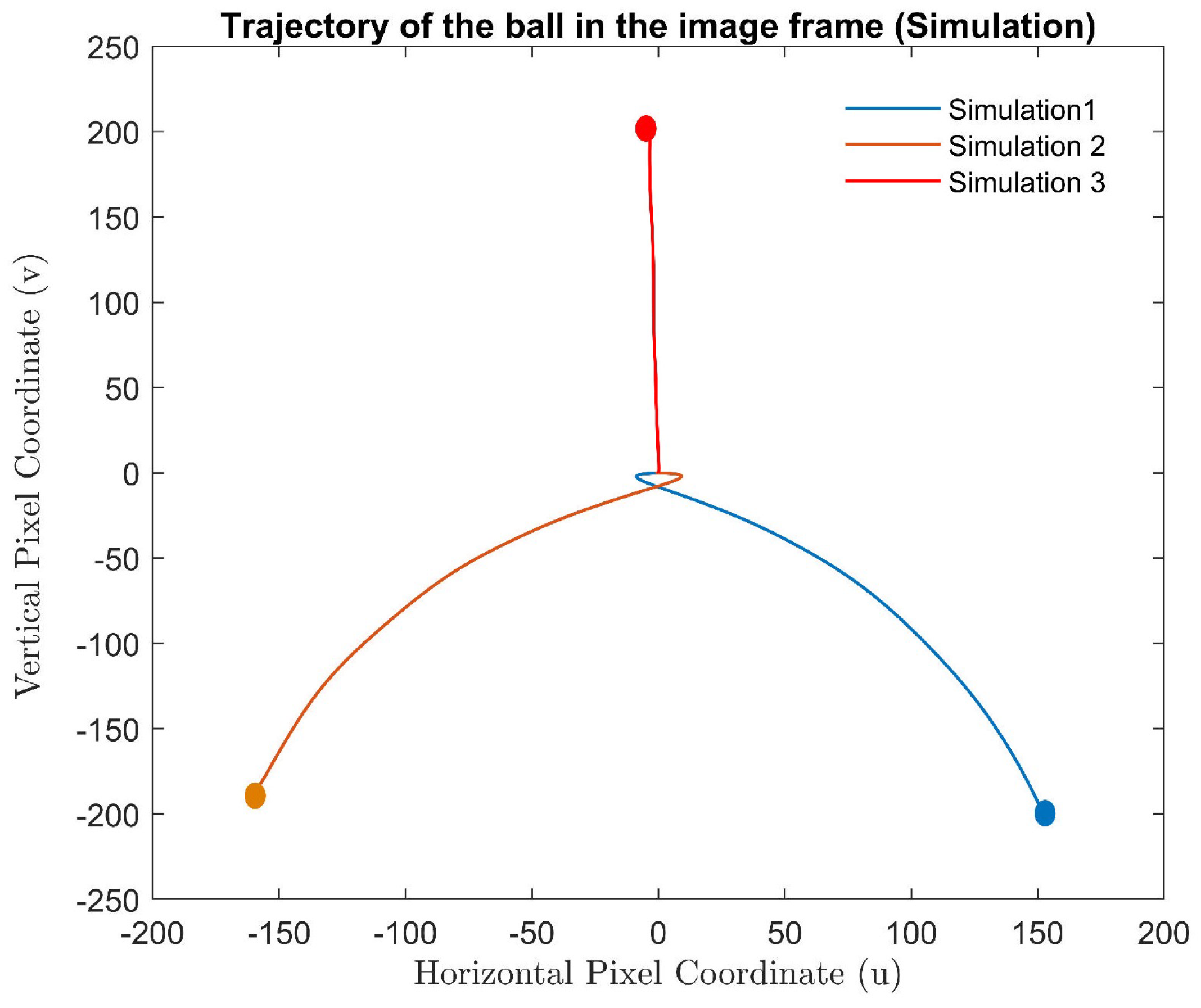
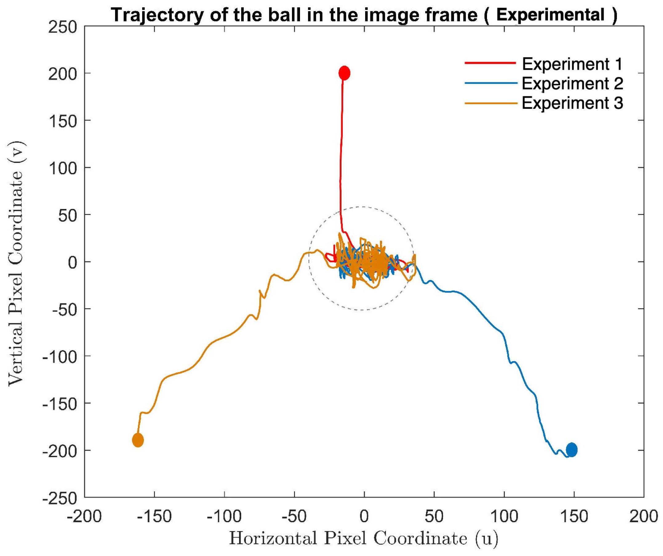
Figure 6 shows the image trajectories of the centroid of the ball for three different simulations. In these simulations, the balls were placed at different initial locations. Furthermore, the experimental results of servoing from the same initial target locations are presented in Figure 7. As seen in the figures, the proposed method was able to servo towards the ball, bringing its image to the centre point.

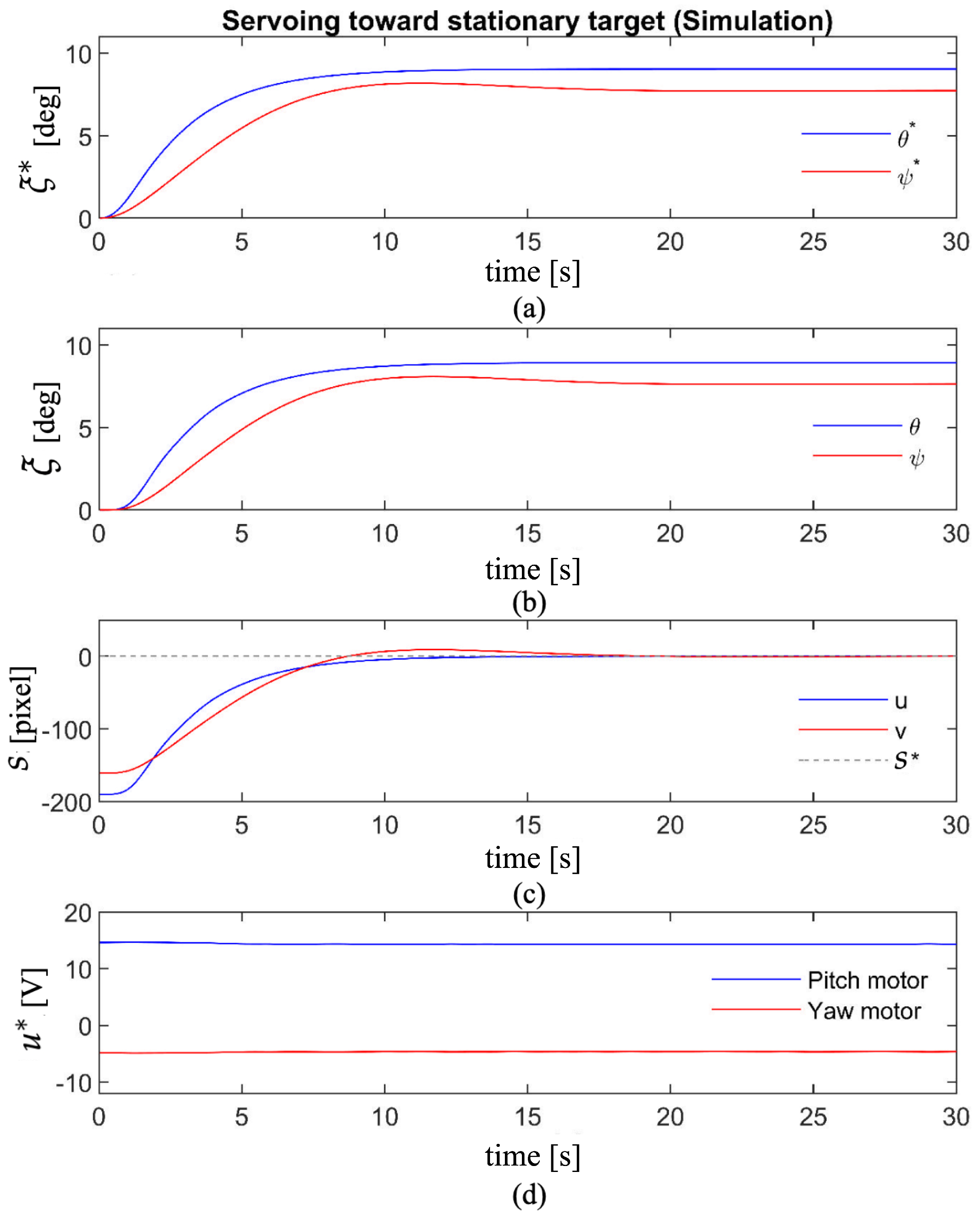
Figure 8 represents the simulated results of servoing toward a stationary target that is initially projected on $S_0=\left[u_0{v}_0\right]=[-184,-165]$ pixels in the image frame. Figure 8a shows $q^{*}$, the desired trajectory generated by the “VPC” block, which should be followed then by the helicopter. The desired trajectory generation process by vision MPC is conducted while considering maximum permissible pitch/yaw accelerations of the UAV. The second-tier controller, namely MPC, is responsible for tracking the desired trajectory calculated in the first stage. Figure 8b demonstrates the pitch/yaw trajectory followed by the helicopter. The desired manipulated variables, namely the voltage applied to the pitch/yaw motors, are calculated via the “MPC” block.

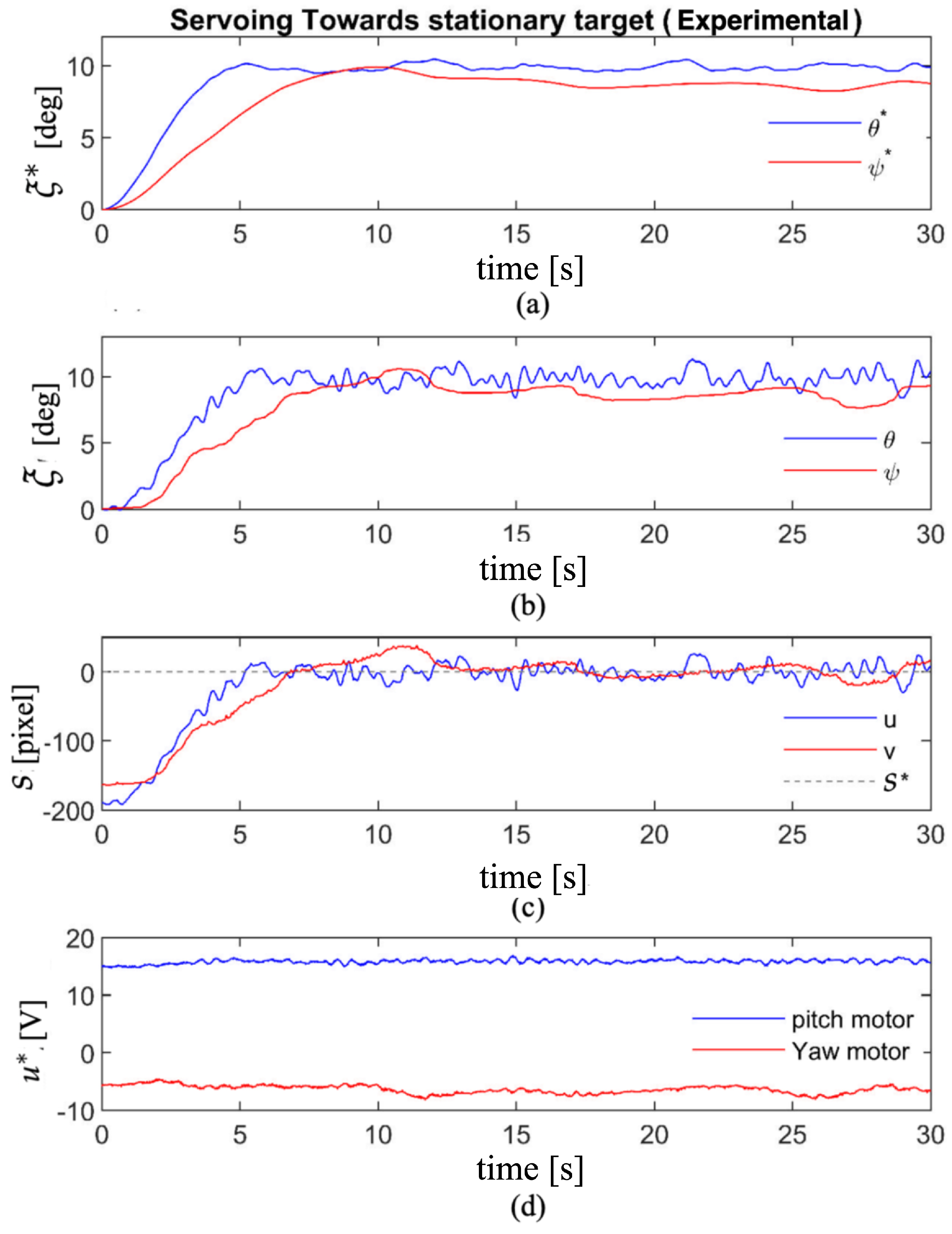
The projected image of the target in the pixel domain converges to the set-point, as seen in Figure 8c. Finally, the control efforts are depicted in Figure 8d. The results of an identical test conducted on the experimental setup are presented in Figure 9a–d. However, some end-of-cycle oscillations exist due to the noise in the image and uncertainties in the helicopter’s motion measurements.

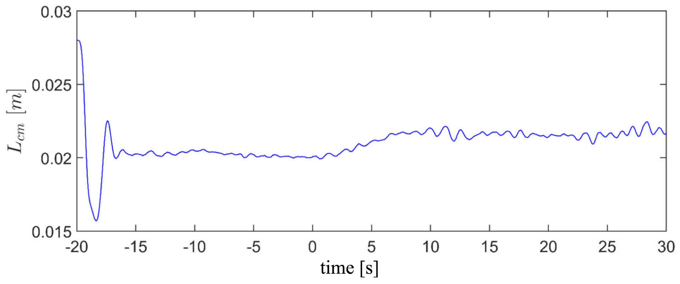
As presented in the system block diagram given in Figure 1, an EKF-based parameter estimator was also implemented to identify the uncertain parameters of the dynamic model in real-time. The estimated dynamic parameters update the prediction model needed by the “MPC”. It is noteworthy that the initial experiments with the system showed that the centre of mass of the helicopter $L_{cm}$ varies during the operation due to effect of data and power cables connected to the system. Figure 10 presents the performance of the system’s parameter estimator in the calculation of the centre of mass of the helicopter. Furthermore, it is worth mentioning that the time coordinate in this plot is referenced to the moment that the VS task begins. However, the MPC and EKF are activated beforehand to bring the target to the field of view of the camera.

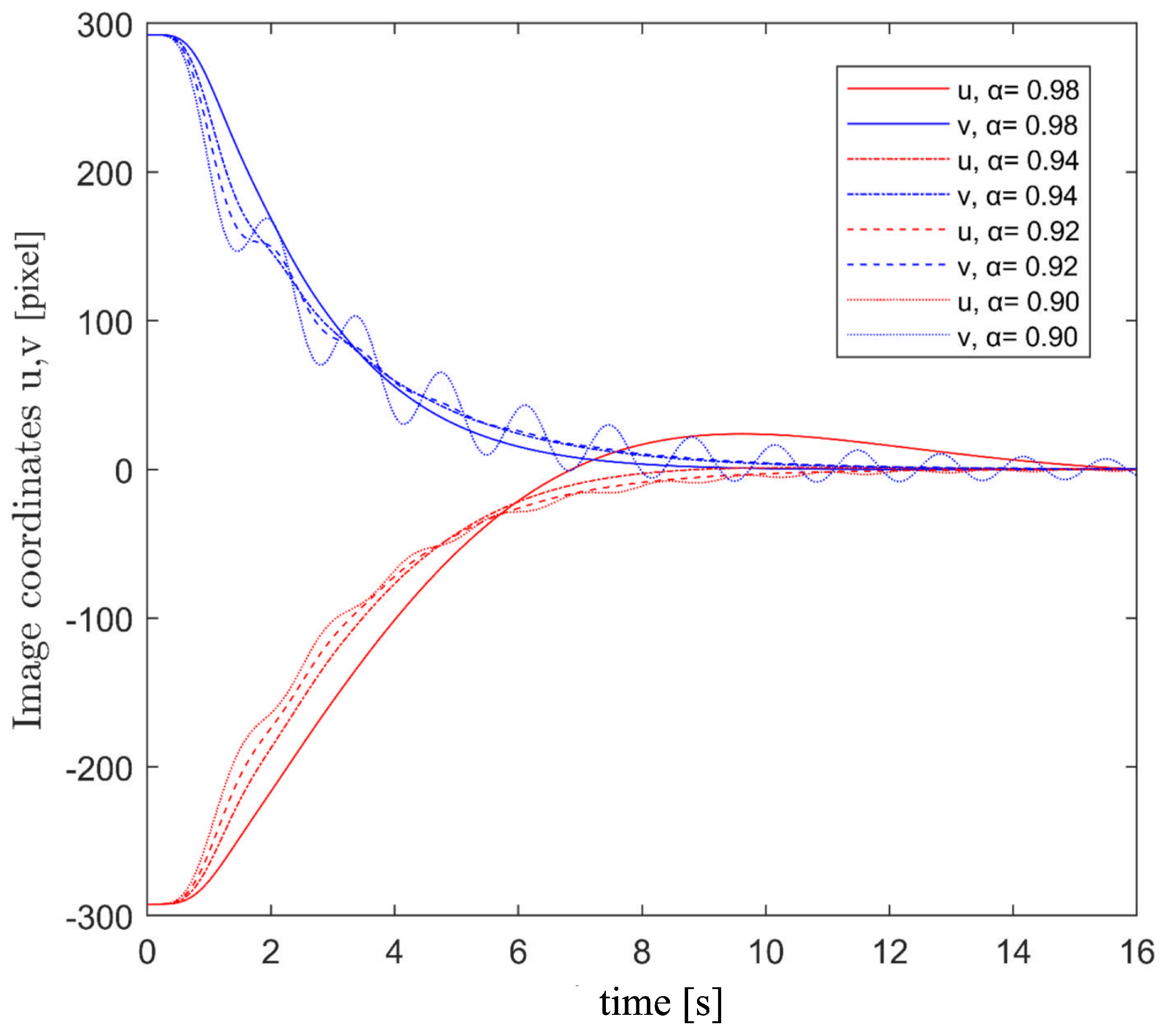
The effect of the tuning parameter used within the Laguerre polynomials, a, the number of utilised network functions, N, and the prediction horizon of the “VPC”, $N_p$, on the overall performance of the proposed algorithm were investigated via simulations (see Figure 11, Figure 12 and Figure 13). According to the results shown in Figure 11, the Laguerre polynomial parameter a has a significant influence on the performance of the proposed servoing algorithm. Additionally, by increasing the number of approximating network polynomials, N, the controller would have improved performance, as shown in Figure 12, but at the cost of an increase in the computational expense. Finally, the effect of the prediction horizon, $N_p$, on the system’s performance is shown in Figure 13. As the results suggest, the shorter the prediction horizon, the smoother the image trajectory will be. However, the system’s response is more agile when predicting further ahead by selecting larger $N_p$.

5. Conclusions

A cascaded two-tier predictive visual servoing approach was formulated under the nonlinear MPC paradigm. The proposed algorithm takes the sensors’, task, and control constraints into consideration. Moreover, the uncertain parameters of the prediction model are estimated through an EKF-based parameter estimator in real-time and updated in each control step, resulting in an adaptive scheme. Furthermore, the control space is parameterised using Laguerre network functions in order to reduce the computational intensity of the algorithm and enable its implementation in real-time. The problem formulated on the 2-DoF model helicopter equipped with a front-facing camera and various simulation and experimental results evaluated the performance and validity of the developed VS approach. In the next research step, we will implement the proposed control method on a free-flying multi-copter. Furthermore, we will improve the control performance against exogenous disturbances such as wind gusts.

References

1. Chaumette, F.; Hutchinson, S. Visual servo control. II. Advanced approaches [Tutorial]. IEEE Robot. Autom. Mag. 2007, 14, 109–118. [Google Scholar] [CrossRef]
2. Fallah, M.M.H.; Janabi-Sharifi, F. Conjugated Visual Predictive Control for Constrained Visual Servoing. J. Intell. Robot. Syst. 2021, 101, 1–21. [Google Scholar]
3. Hutchinson, S.; Hager, G.D.; Corke, P.I. A tutorial on visual servo control. IEEE Trans. Robot. Autom. 1996, 12, 651–670. [Google Scholar] [CrossRef] [Green Version]
4. Allibert, G.; Courtial, E.; Chaumette, F. Predictive control for constrained image-based visual servoing. IEEE Trans. Robot. 2010, 26, 933–939. [Google Scholar] [CrossRef] [Green Version]
5. Gonçalves, P.J.S.; Paris, A.; Christo, C.; Sousa, J.; Pinto, J.C. Uncalibrated visual servoing in 3d workspace. In Proceedings of the International Conference Image Analysis and Recognition, Póvoa de Varzim, Portugal, 18–20 September 2006; pp. 225–236. [Google Scholar]
6. Jagersand, M.; Fuentes, O.; Nelson, R. Experimental evaluation of uncalibrated visual servoing for precision manipulation. In Proceedings of the International Conference on Robotics and Automation, Albuquerque, NM, USA, 20–25 April 1997; Volume 4, pp. 2874–2880. [Google Scholar]
7. Xu, F.; Wang, H.; Liu, Z.; Chen, W. Adaptive Visual Servoing for an Underwater Soft Robot Considering Refraction Effects. IEEE Trans. Ind. Electron. 2019, 67, 10575–10586. [Google Scholar] [CrossRef]
8. Assa, A. Robust Robotic Visual Servoing for Uncertain Systems. Ph.D. Thesis, Ryerson University, Toronto, ON, Canada, 2015. [Google Scholar]
9. Kelly, R. Robust asymptotically stable visual servoing of planar robots. IEEE Trans. Robot. Autom. 1996, 12, 759–766. [Google Scholar] [CrossRef]
10. Seo, H.; Kim, S.; Kim, H.J. Aerial grasping of cylindrical object using visual servoing based on stochastic model predictive control. In Proceedings of the 2017 IEEE International Conference on Robotics and Automation (ICRA), Singapore, 29 May–3 June 2017; pp. 6362–6368. [Google Scholar]
11. Ghasemi, A. Enhanced Image-Based Visual Servoing Dealing with Uncertainties. Ph.D. Thesis, Concordia University, Montreal, QC, Canada, 2020. [Google Scholar]
12. Zhakatayev, A.; Rakhim, B.; Adiyatov, O.; Baimyshev, A.; Varol, H.A. Successive linearization based model predictive control of variable stiffness actuated robots. In Proceedings of the 2017 IEEE International Conference on Advanced Intelligent Mechatronics (AIM), Munich, Germany, 3–7 July 2017; pp. 1774–1779. [Google Scholar]
13. Caldwell, J.; Marshall, J.A. Towards Efficient Learning-Based Model Predictive Control via Feedback Linearization and Gaussian Process Regression. In Proceedings of the 2021 IEEE/RSJ International Conference on Intelligent Robots and Systems (IROS), Prague, Czech Republic, 27 September–1 October 2021; pp. 4306–4311. [Google Scholar]
14. Gulan, M.; Minarčík, P. Implementation of continuous-time MPC using B-spline functions. In Proceedings of the 2019 22nd International Conference on Process Control (PC19), Strbske Pleso, Slovakia, 11–14 June 2019; pp. 222–227. [Google Scholar]
15. Valencia-Palomo, G.; Rossiter, J.A. Using Laguerre functions to improve efficiency of multi-parametric predictive control. In Proceedings of the 2010 American Control Conference, Baltimore, MD, USA, 30 June–2 July 2010; pp. 4731–4736. [Google Scholar]
16. Khan, B.; Rossiter, J.A.; Valencia-Palomo, G. Exploiting Kautz functions to improve feasibility in MPC. IFAC Proc. Vol. 2011, 44, 6777–6782. [Google Scholar] [CrossRef] [Green Version]
17. Sajjadi, S.; Mehrandezh, M.; Janabi-Sharifi, F. A Nonlinear Adaptive Model-Predictive Approach for Visual Servoing of Unmanned Aerial Vehicles. In Progress in Optomechatronic Technologies; Springer Proceedings in Physics Book Series; Springer: Berlin, Germany, 2019; pp. 153–164. [Google Scholar] [CrossRef]
18. Zhang, Z. A flexible new technique for camera calibration. IEEE Trans. Pattern Anal. Mach. Intell. 2000, 22, 1330–1334. [Google Scholar] [CrossRef] [Green Version]
19. Wang, L. Model Predictive Control System Design and Implementation Using MATLAB; Springer: Berlin, Germany, 2009. [Google Scholar]
20. Kim, Y.; Bang, H. Introduction to Kalman Filter and Its Applications. In Introduction to Kalman Filter and Its Applications; IntechOpen: London, UK, 2018. [Google Scholar]
21. Carrassi, A.; Vannitsem, S. State and parameter estimation with the extended Kalman filter: An alternative formulation of the model error dynamics. Q. J. R. Meteorol. Soc. 2011, 137, 435–451. [Google Scholar] [CrossRef]
22. Sun, X.; Jin, L.; Xiong, M. Extended Kalman filter for estimation of parameters in nonlinear state-space models of biochemical networks. PLoS ONE 2008, 3, e3758. [Google Scholar] [CrossRef] [PubMed]
23. Varshney, D.; Bhushan, M.; Patwardhan, S.C. State and parameter estimation using extended Kalman filter. J. Process Control 2019, 76, 98–111. [Google Scholar] [CrossRef]
24. Assa, A.; Janabi-Sharifi, F. Robust model predictive control for visual servoing. In Proceedings of the 2014 IEEE/RSJ International Conference on Intelligent Robots and Systems, Chicago, IL, USA, 14–18 September 2014; pp. 2715–2720. [Google Scholar]
25. Reina, G.; Messina, A. Vehicle Dynamics Estimation via Augmented Extended Kalman Filtering. Measurement 2018, 133, 383–395. [Google Scholar] [CrossRef]
26. Patel, R.; Deb, D.; Modi, H.; Shah, S. Adaptive backstepping control scheme with integral action for quanser 2-dof helicopter. In Proceedings of the 2017 International Conference on Advances in Computing, Communications and Informatics (ICACCI), Manipal, India, 13–16 September 2017; pp. 571–577. [Google Scholar]
27. Quanser. 2022. Available online: https://www.quanser.com/ (accessed on 5 January 2022).
28. Logitech. 2022. Available online: https://www.logitech.com/en-ca/products/webcams/c270-hd-webcam.960-000694.html/ (accessed on 3 January 2022).
29. Corke, P. Robotics, Vision and Control: Fundamental Algorithms in MATLAB®, 2nd ed.; Springer: Berlin, Germany, 2017. [Google Scholar]
30. Assa, A.; Janabi-Sharifi, F. Hybrid predictive control for constrained visual servoing. In Proceedings of the 2014 IEEE/ASME International Conference on Advanced Intelligent Mechatronics, Besançon, France, 8–11 July 2014; pp. 931–936. [Google Scholar]
31. Single Camera Calibrator App—MATLAB & Simulink. 2018. Available online: https://www.mathworks.com/help/vision/ug/single-camera-calibrator-app.html (accessed on 1 March 2021).
32. Chaumette, F.; Hutchinson, S.; Corke, P. Visual servoing. In Springer Handbook of Robotics; Springer: Berlin, Germany, 2016; pp. 841–866. [Google Scholar]
33. Gongye, Q.; Cheng, P.; Dong, J. Image-based visual servoing with depth estimation. Trans. Inst. Meas. Control 2022, 44, 1811–1823. [Google Scholar] [CrossRef]
34. De Luca, A.; Oriolo, G.; Giordano, P.R. On-line estimation of feature depth for image-based visual servoing schemes. In Proceedings of the 2007 IEEE International Conference on Robotics and Automation, Roma, Italy, 10–14 April 2007; pp. 2823–2828. [Google Scholar]
35. MATLAB. Webcam Support from MATLAB and Simulink. 2022. Available online: https://www.mathworks.com/hardware-support/webcam.html (accessed on 5 May 2022).
36. MATLAB. Computer Vision with Simulink. 2022. Available online: https://www.mathworks.com/help/vision/computer-vision-with-simulink.html (accessed on 5 May 2022).
37. MATLAB. MATLAB Function Blocks. 2022. Available online: https://www.mathworks.com/help/simulink/ug/what-is-a-matlab-function-block.html (accessed on 5 May 2022).
Figure 1. The architecture of the proposed two-stage controller.
Drones 06 00127 g001
Figure 3. Logitech camera, ping-pong ball, and high-contrast blue background.
Drones 06 00127 g003
Figure 4. Location of the global coordinates frame with respect to the image frame.
Drones 06 00127 g004
Figure 5. The image processing steps: (a) image captured by the camera; (b) colour threshold in the HSV space; (c) result of the blob size filter; (d) centre of the ball and camera marked.
Drones 06 00127 g005
Figure 6. Simulations with different initial locations of the target and the corresponding trajectory in the image frame.
Drones 06 00127 g006
Figure 7. Experiments with different initial locations of the target and the corresponding trajectory in the image frame.
Drones 06 00127 g007
Figure 8. Servoing toward stationary target (simulation): (a) the trajectory generated by VPC; (b) the trajectory followed by the UAV; (c) the feature error in the image frame; (d) the inputs applied to the pitch/yaw motors.
Drones 06 00127 g008
Figure 9. Servoing toward stationary target (experimental): (a) the trajectory generated by VPC; (b) the trajectory followed by the UAV; (c) the feature error in the image frame; (d) the inputs applied to the pitch/yaw motors.
Drones 06 00127 g009
Figure 10. Centre of mass of the helicopter L c m estimated by the EKF parameter estimator.
Drones 06 00127 g010
Figure 11. The effect of parameter a of the Laguerre network functions on the control performance (simulation).
Drones 06 00127 g011
Figure 12. The influence of the number of Laguerre polynomials on servoing performance (simulation).
Drones 06 00127 g012
Figure 13. The influence of prediction horizon N p on servoing toward the stationary target (simulation).
Drones 06 00127 g013