
Investigation of Rotor Efficiency with Varying Rotor Pitch Angle for a Coaxial Drone


Abstract
:1. Introduction
2. Computational Methods
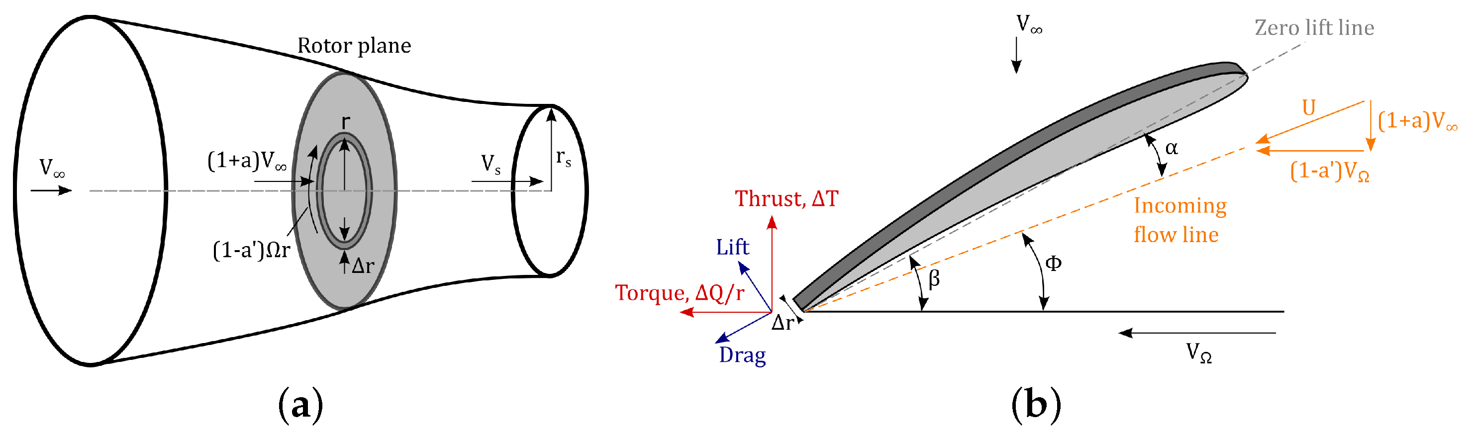
2.1. Blade Element Momentum Theory
2.2. Computational Fluid Dynamics
3. Numerical Setup
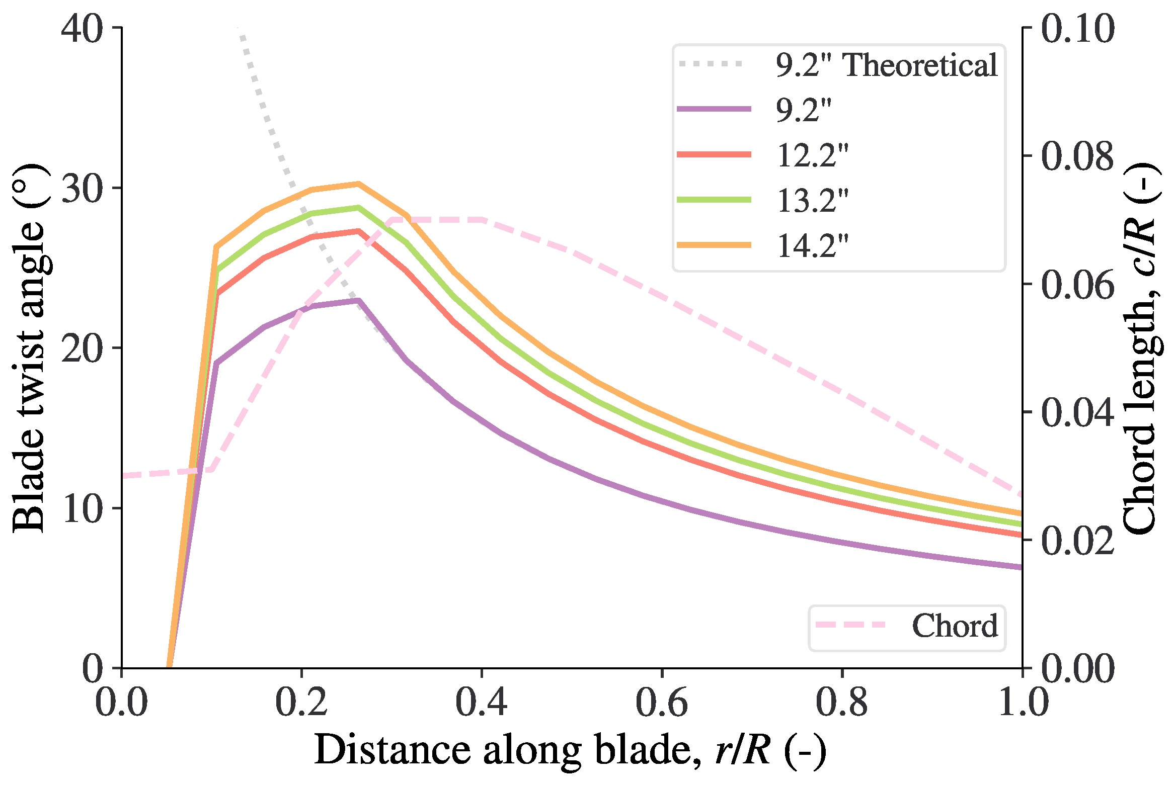
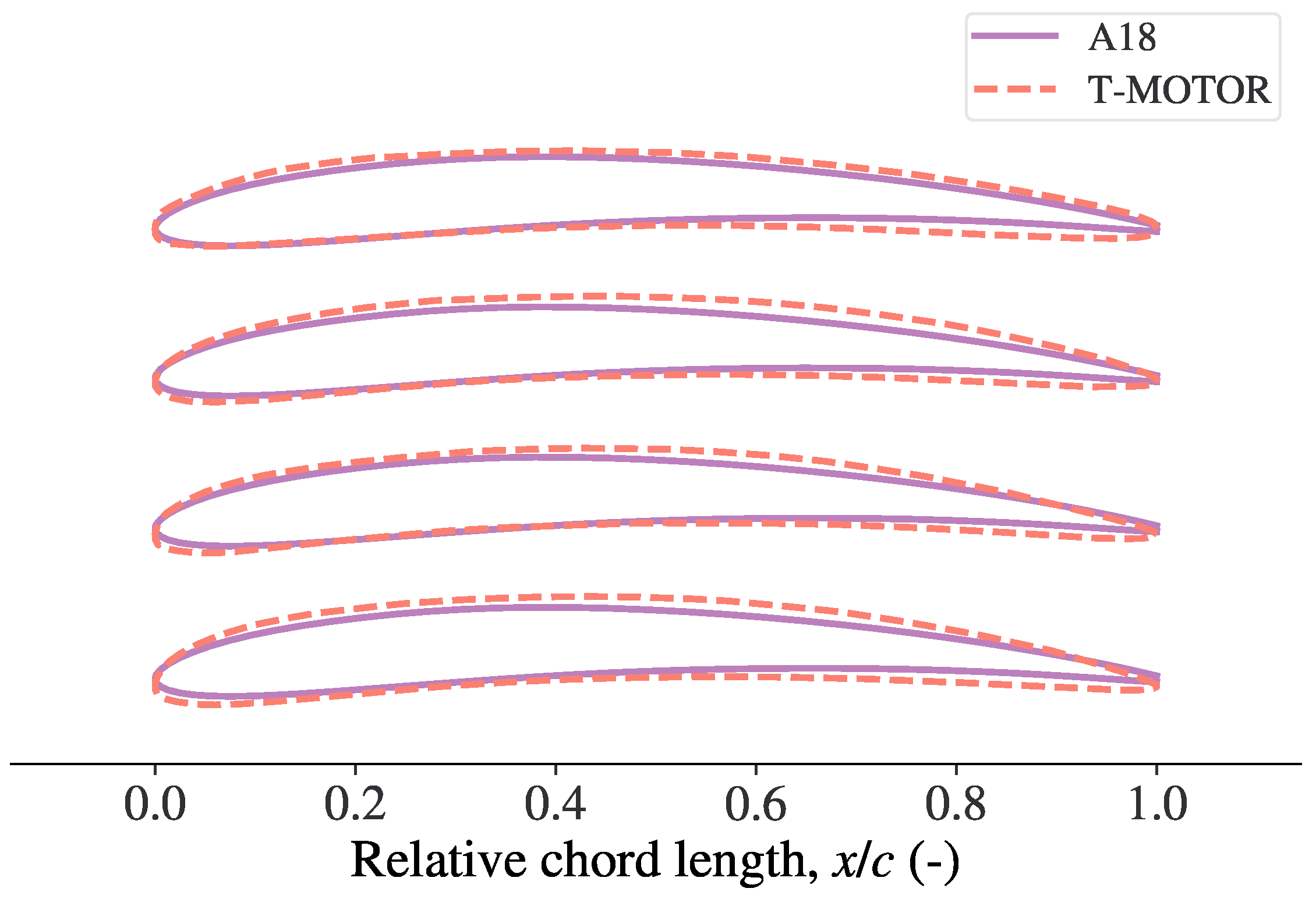
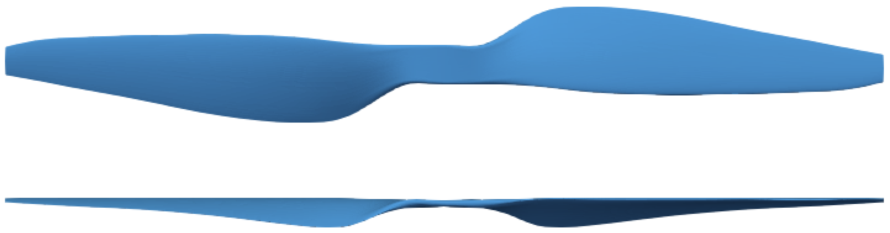
3.1. Rotor Geometry
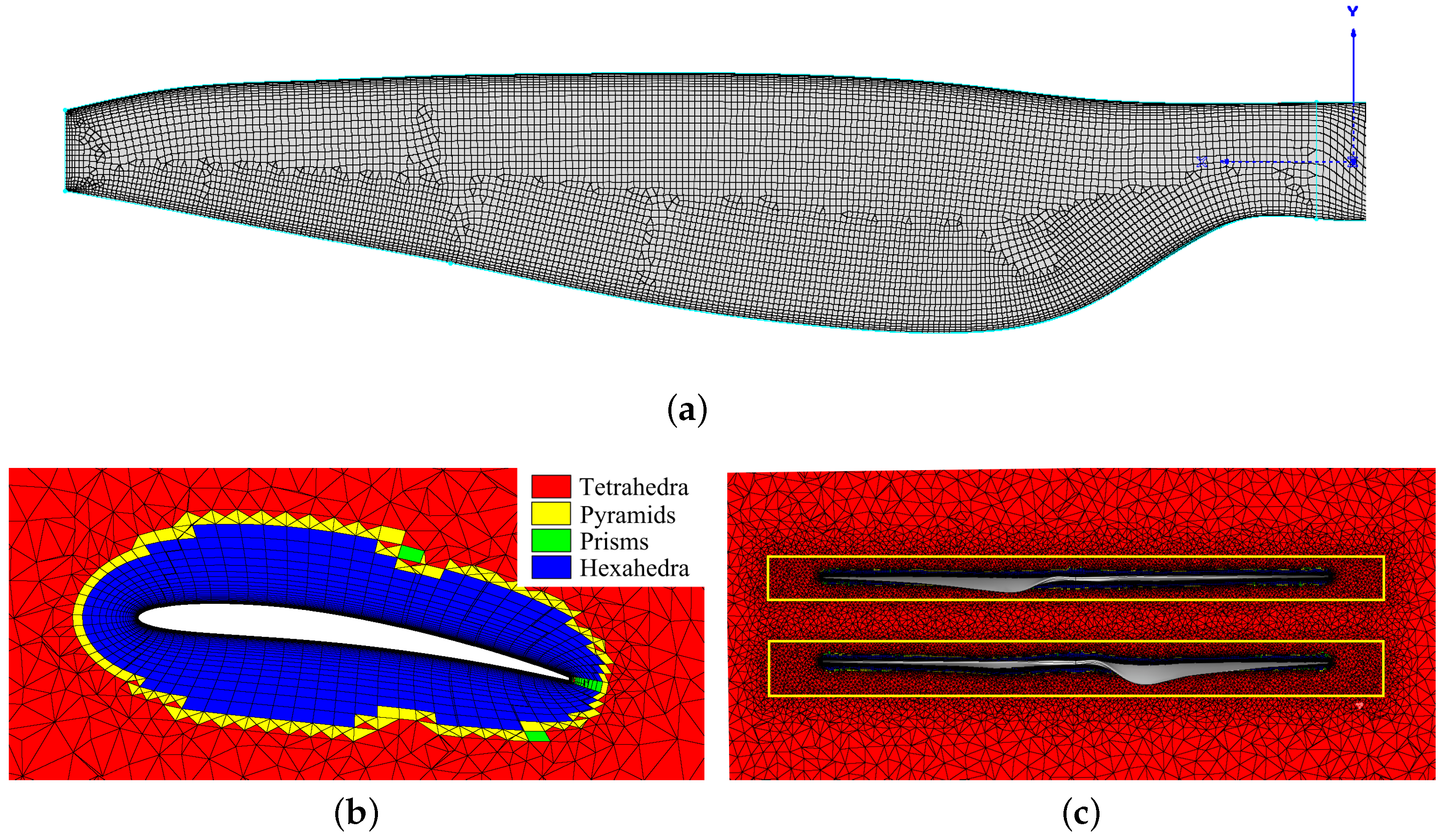
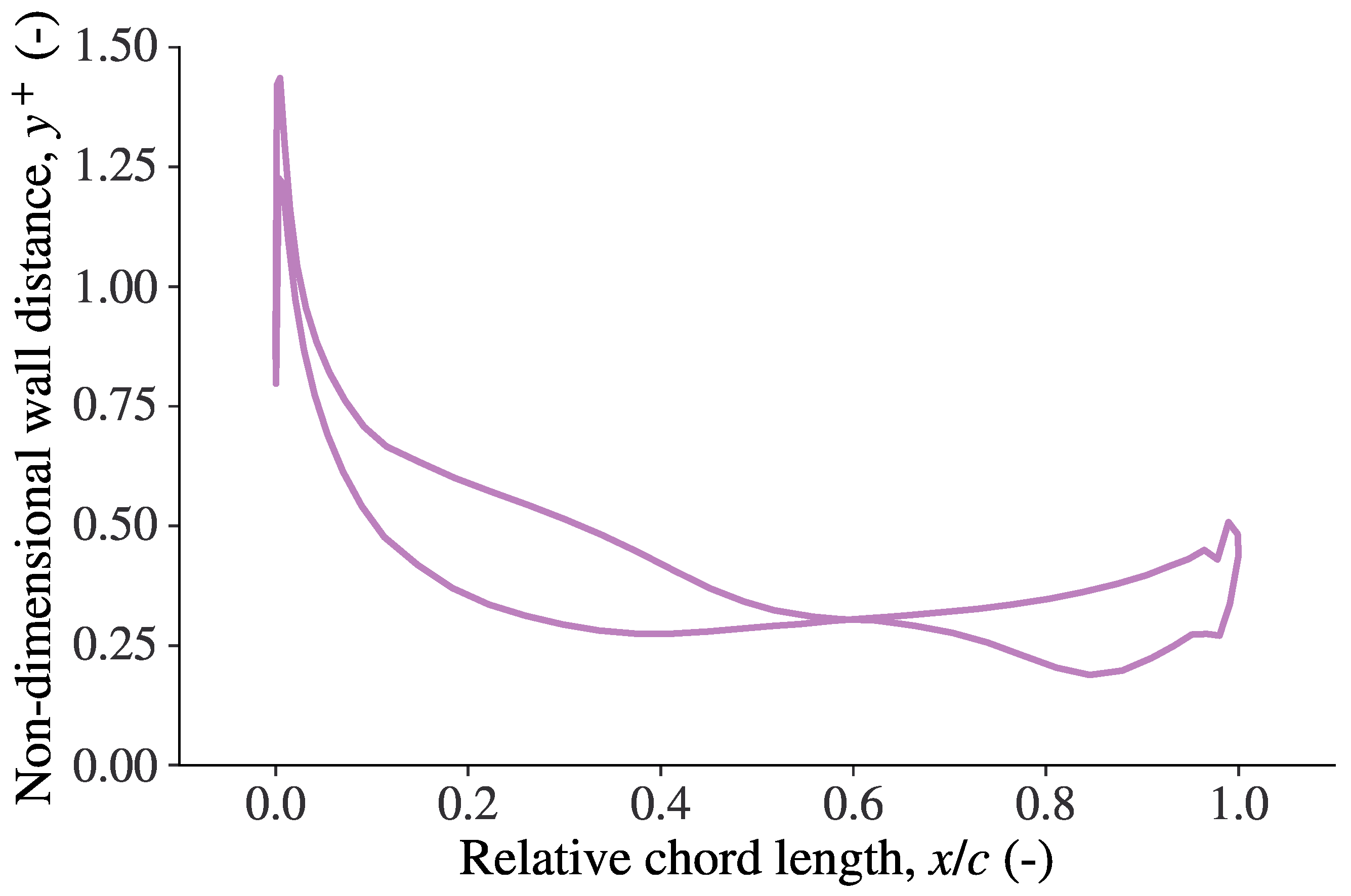
3.2. Mesh
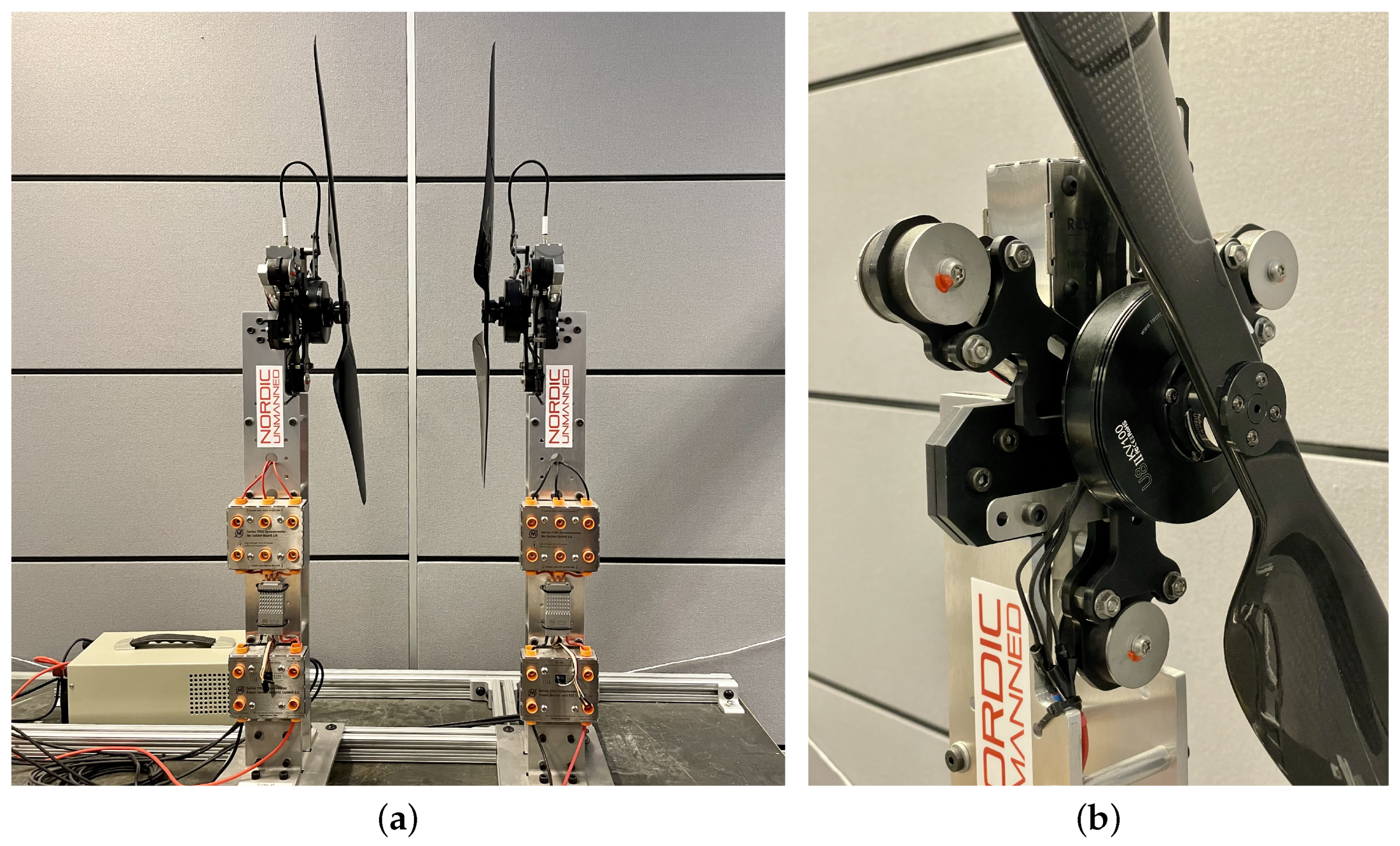
4. Experimental Setup
5. Validation
5.1. Mesh Sensitivity Study
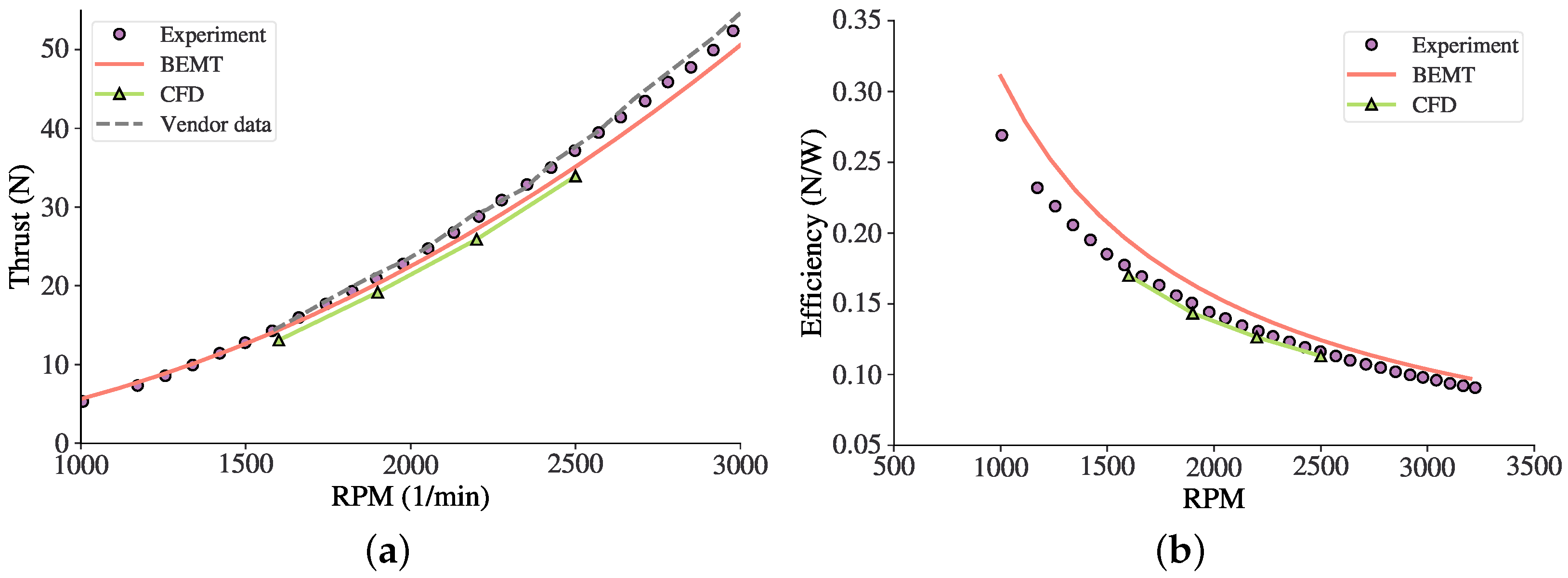
5.2. Single-Rotor Validation
5.3. Coaxial Rotor Validation
6. Results
7. Conclusions
Author Contributions
Funding
Data Availability Statement
Acknowledgments
Conflicts of Interest
References
- Hassanalian, M.; Abdelkefi, A. Classifications, applications, and design challenges of drones: A review. Prog. Aerosp. Sci. 2017, 91, 99–131. [Google Scholar] [CrossRef]
- Miiller, H.; Palossi, D.; Mach, S.; Conti, F.; Benini, L. Fünfiiber-Drone: A Modular Open-Platform 18-grams Autonomous Nano-Drone. In Proceedings of the Design, Automation & Test in Europe Conference & Exhibition, Virtual, 1–5 February 2021; pp. 1610–1615. [Google Scholar]
- Giernacki, W.; Skwierczyński, M.; Witwicki, W.; Wroński, P.; Kozierski, P. Crazyflie 2.0 quadrotor as a platform for research and education in robotics and control engineering. In Proceedings of the 22nd International Conference on Methods and Models in Automation and Robotics (MMAR), Miedzyzdroje, Poland, 28–31 August 2017; pp. 37–42. [Google Scholar]
- Shamiyeh, M.; Rothfeld, R.; Hornung, M. A performance benchmark of recent personal air vehicle concepts for urban air mobility. In Proceedings of the 31st Congress of the International Council of the Aeronautical Sciences, Belo Horizonte, Brazil, 9–14 September 2018; Volume 14. [Google Scholar]
- Moore, M.D. Personal Air Vehicle Exploration (PAVE); NASA Langley Research Center: Hampton, VI, USA, 2002; pp. 1–48.
- Bradley, T.H.; Moffitt, B.A.; Fuller, T.F.; Mavris, D.N.; Parekh, D.E. Comparison of design methods for fuel-cell-powered unmanned aerial vehicles. J. Aircraft 2009, 46, 1945–1956. [Google Scholar] [CrossRef]
- Apeland, J. Use of Fuel Cells to Extend Multirotor Drone Endurance. Ph.D. Thesis, University of Stavanger, Stavanger, Norway, 2021. [Google Scholar]
- Prior, S.D. Reviewing and investigating the use of Co-Axial rotor systems in small UAVs. Int. J. Micro Air Veh. 2010, 2, 1–16. [Google Scholar] [CrossRef]
- Lei, Y.; Ji, Y.; Wang, C. Optimization of aerodynamic performance for co-axial rotors with different rotor spacings. Int. J. Micro Air Veh. 2018, 10, 362–369. [Google Scholar] [CrossRef]
- Brazinskas, M.; Prior, S.D.; Scanlan, J.P. An empirical study of overlapping rotor interference for a small unmanned aircraft propulsion system. Aerospace 2016, 3, 32. [Google Scholar] [CrossRef]
- Weishäupl, A.B.; Prior, S.D. Influence of Propeller Overlap on Large-Scale Tandem UAV Performance. Unmanned Sys. 2019, 7, 245–260. [Google Scholar] [CrossRef]
- Prior, S.D. Optimizing Small Multi-Rotor Unmanned Aircraft: A Practical Design Guide; CRC Press: Boca Raton, FL, USA, 2018. [Google Scholar]
- Yoon, S.; Chan, W.M.; Pulliam, T.H. Computations of torque-balanced coaxial rotor flows. In Proceedings of the 55th AIAA Aerospace Sciences Meeting, Grapevine, TX, USA, 9–13 January 2017; p. 52. [Google Scholar]
- Jinghui, D.; Feng, F.; Huang, S.; Yongfeng, L. Aerodynamic characteristics of rigid coaxial rotor by wind tunnel test and numerical calculation. Chin. J. Aeronaut. 2019, 32, 568–576. [Google Scholar]
- Kim, Y.T.; Park, C.H.; Kim, H.Y. Three-Dimensional CFD Investigation of Performance and Interference Effect of Coaxial Propellers. In Proceedings of the IEEE 10th International Conference on Mechanical and Aerospace Engineering (ICMAE), Brussels, Belgium, 22–25 July 2019; pp. 376–383. [Google Scholar]
- Leishman, J.G.; Ananthan, S. An optimum coaxial rotor system for axial flight. J. Am. Helicopter Soc. 2008, 53, 366–381. [Google Scholar] [CrossRef]
- Leishman, G.J. Principles of Helicopter Aerodynamics; Cambridge University Press: Cambridge, UK, 2006. [Google Scholar]
- Manwell, J.F.; McCowan, J.; Rogers, A.L. Wind energy explained: Theory, design and application. Wind Eng. 2006, 30, 169. [Google Scholar]
- Schmitz, S. Aerodynamics of Wind Turbines: A Physical Basis for Analysis and Design; John Wiley & Sons: Hoboken, NJ, USA, 2020. [Google Scholar]
- Glauert, H. Airplane propellers. In Aerodynamic Theory; Springer: Berlin/Heidelberg, Germany, 1935; pp. 169–360. [Google Scholar]
- Giljarhus, K.E.T. pyBEMT: An implementation of the Blade Element Momentum Theory in Python. J. Open Source Softw. 2020, 5, 2480. [Google Scholar] [CrossRef]
- Virtanen, P.; Gommers, R.; Oliphant, T.E.; Haberland, M.; Reddy, T.; Cournapeau, D.; Burovski, E.; Peterson, P.; Weckesser, W.; Bright, J.; et al. SciPy 1.0: Fundamental Algorithms for Scientific Computing in Python. Nat. Methods 2020, 17, 261–272. [Google Scholar] [CrossRef] [PubMed] [Green Version]
- Leishman, J.G.; Syal, M. Figure of merit definition for coaxial rotors. J. Am. Helicopter Soc. 2008, 53, 290–300. [Google Scholar] [CrossRef]
- Lee, S.; Dassonville, M. Iterative Blade Element Momentum Theory for Predicting Coaxial Rotor Performance in Hover. J. Am. Helicopter Soc. 2020, 65, 1–12. [Google Scholar] [CrossRef]
- Lakshminarayan, V.K.; Baeder, J.D. Computational investigation of microscale coaxial-rotor aerodynamics in hover. J. Aircr. 2010, 47, 940–955. [Google Scholar] [CrossRef] [Green Version]
- Yoon, S.; Chaderjian, N.; Pulliam, T.H.; Holst, T. Effect of turbulence modeling on hovering rotor flows. In Proceedings of the 45th AIAA Fluid Dynamics Conference, Dallas, TX, USA, 22–26 June 2015; p. 2766. [Google Scholar]
- Lopez, O.D.; Escobar, J.A.; Pérez, A.M. Computational study of the wake of a quadcopter propeller in hover. In Proceedings of the 23rd AIAA Computational Fluid Dynamics Conference, Denver, CO, USA, 5–9 June 2017; p. 3961. [Google Scholar]
- Loureiro, E.V.; Oliveira, N.L.; Hallak, P.H.; de Souza Bastos, F.; Rocha, L.M.; Delmonte, R.G.P.; de Castro Lemonge, A.C. Evaluation of low fidelity and CFD methods for the aerodynamic performance of a small propeller. Aerosp. Sci. Tech. 2021, 108, 106402. [Google Scholar] [CrossRef]
- Barbely, N.L.; Komerath, N.M.; Novak, L.A. A Study of Coaxial Rotor Performance and Flow Field Characteristics. In Proceedings of the 2016 AHS Technical Meeting on Aeromechanics Design for Vertical Lift, San Francisco, CA, USA, 20–22 January 2016. [Google Scholar]
- Cornelius, J.K.; Schmitz, S.; Kinzel, M.P. Efficient computational fluid dynamics approach for coaxial rotor simulations in hover. J. Aircraft 2020, 58, 197–203. [Google Scholar] [CrossRef]
- Panjwani, B.; Quinsard, C.; Przemysław, D.G.; Furseth, J. Virtual Modelling and Testing of the Single and Contra-Rotating Co-Axial Propeller. Drones 2020, 4, 42. [Google Scholar] [CrossRef]
- Menter, F.R. Two-equation eddy-viscosity turbulence models for engineering applications. AIAA J. 1994, 32, 1598–1605. [Google Scholar] [CrossRef] [Green Version]
- Weller, H.G.; Tabor, G.; Jasak, H.; Fureby, C. A tensorial approach to computational continuum mechanics using object-oriented techniques. Comput. Phys. 1998, 12, 620–631. [Google Scholar] [CrossRef]
- Jasak, H.; Jemcov, A.; Tukovic, Z. OpenFOAM: A C++ Library for Complex Physics Simulations; CMND. IUC: Dubrovnik, Croatia, 2007; Volume 1000. [Google Scholar]
- Farrell, P.; Maddison, J. Conservative interpolation between volume meshes by local Galerkin projection. Comput. Method Appl. Mech. Eng. 2011, 200, 89–100. [Google Scholar] [CrossRef]
- Nordic Unmanned. Staaker BG-200. Available online: https://nordicunmanned.com/drones/staaker-bg200/ (accessed on 10 March 2022).
- PRODRONE. PD6B-Type2. Available online: https://www.prodrone.com/products/pd6b-type2/ (accessed on 10 March 2022).
- Czerhoniak, M.S. Scaling up the Propulsion System of an Aerial and Submersible Multirotor Vehicle. Ph.D. Thesis, Rutgers University-School of Graduate Studies, Piscataway, NJ, USA, 2018. [Google Scholar]
- Selig, M.S. Summary of Low Speed Airfoil Data; SOARTECH Publications: Virginia Beach, VI, USA, 1995. [Google Scholar]
- Selig, M.S. UIUC Airfoil Data Site. 1996. Available online: https://m-selig.ae.illinois.edu/ads.html (accessed on 10 March 2022).
- Drela, M. XFOIL: An analysis and design system for low reynolds number airfoils. In Low Reynolds Number Aerodynamics; Springer: Berlin/Heidelberg, Germany, 1989; pp. 1–12. [Google Scholar]
- Marten, D.; Wendler, J.; Pechlivanoglou, G.; Nayeri, C.N.; Paschereit, C.O. QBLADE: An open source tool for design and simulation of horizontal and vertical axis wind turbines. Int. J. Emer. Tech. Adv. Eng. 2013, 3, 264–269. [Google Scholar]
- Cadence Design Systems. Pointwise® V18.4R4. Available online: https://www.pointwise.com (accessed on 25 December 2021).
- T-MOTOR. T-MOTOR U8II. Available online: https://store.tmotor.com/goods.php?id=476 (accessed on 8 February 2019).
- Cabral, B.; Leedom, L.C. Imaging vector fields using line integral convolution. In Proceedings of the 20th Annual Conference on Computer Graphics and Interactive Techniques, Anaheim, CA, USA, 2–6 August 1993; pp. 263–270. [Google Scholar]


| Quantity | Unit | Value |
|---|---|---|
| Rotor diameter, D | cm | 71.12 |
| Number of blades | - | 2 |
| Hub diameter | cm | 5.4 |
| Pitch at 0.75R | in | 9.2 |
| Chord at 0.75R | cm | 4.4 |
| Object | Base Diameter | Height | Ratio to D |
|---|---|---|---|
| Upper AMI block | 84.0 cm | 5.50 cm | |
| Lower AMI block | 84.0 cm | 6.95 cm | |
| Cylindrical source | 1.00 m | 3.00 m | |
| Far-field block | 10.0 m | 10.0 m |
| Quantity | Unit | Value | Ratio to D |
|---|---|---|---|
| Rotor surface maximum cell size | mm | 2.00 | |
| 3D T-Rex 1st layer thickness | m | 1 × 10⁻⁵ | |
| 3D T-Rex inflation growth factor | - | 1.2 | |
| AMI block maximum cell size | mm | 5.00 | |
| Source delimited region max. cell size | cm | 2.00 | |
| Far-field block maximum cell size | cm | 20.0 | |
| Total number of cells | - | 14.1 × 10⁶ |
| Number of Cells | Thrust | Efficiency |
|---|---|---|
| (×106) | (N) | (N W−1) |
| 5.50 | 25.5 | 0.124 |
| 8.78 | 25.9 | 0.127 |
| 13.2 | 26.0 | 0.127 |
Publisher’s Note: MDPI stays neutral with regard to jurisdictional claims in published maps and institutional affiliations. |
© 2022 by the authors. Licensee MDPI, Basel, Switzerland. This article is an open access article distributed under the terms and conditions of the Creative Commons Attribution (CC BY) license (https://creativecommons.org/licenses/by/4.0/).
Share and Cite
Giljarhus, K.E.T.; Porcarelli, A.; Apeland, J. Investigation of Rotor Efficiency with Varying Rotor Pitch Angle for a Coaxial Drone. Drones 2022, 6, 91. https://doi.org/10.3390/drones6040091
Giljarhus KET, Porcarelli A, Apeland J. Investigation of Rotor Efficiency with Varying Rotor Pitch Angle for a Coaxial Drone. Drones. 2022; 6(4):91. https://doi.org/10.3390/drones6040091
Chicago/Turabian StyleGiljarhus, Knut Erik Teigen, Alessandro Porcarelli, and Jørgen Apeland. 2022. "Investigation of Rotor Efficiency with Varying Rotor Pitch Angle for a Coaxial Drone" Drones 6, no. 4: 91. https://doi.org/10.3390/drones6040091
APA StyleGiljarhus, K. E. T., Porcarelli, A., & Apeland, J. (2022). Investigation of Rotor Efficiency with Varying Rotor Pitch Angle for a Coaxial Drone. Drones, 6(4), 91. https://doi.org/10.3390/drones6040091