1. Introduction
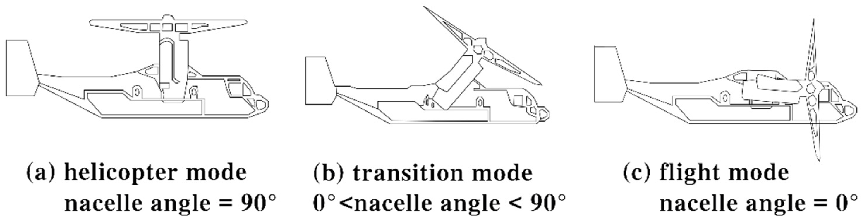
A tiltrotor is an important derivative of short take-off and vertical landing (STOVL) aircraft. As a hybrid vehicle, it combines the merits of both a helicopter and a fixed-wing aircraft. It can hover and vertically take off and land like a helicopter and fly forward fast like a fixed-wing aircraft. A tiltrotor has a nacelle installed at every wingtip. The nacelle can tilt 0–90° and switch from helicopter mode and transition mode to flight mode. A tiltrotor has many flight modes as
Figure 1 and thus is granted with wide flight envelope, which brings great development potential but also many technical issues [
1,
2,
3,
4,
5,
6]. For example, there is airflow disturbance between the rotor and the wing; the aerodynamic parameters of the aircraft change sharply in the transition section of the tiltrotor aircraft; and there are problems such as redundancy of multiple control surfaces, large aerodynamic coupling between different channels of the tilt rotor aircraft, and poor aerodynamic stability during high-speed flight. Due to its complexity in terms of dynamics, building a complete mathematical model becomes significant for designing the flight control system, which justifies its difficulty as well. This is why mathematical modeling is a critical technical issue for a tiltrotor.
Reference [
7] investigates optimal tiltrotor flight trajectories considering the possibility of engine failure. A two-dimensional longitudinal rigid body model of a tiltrotor aircraft is used. It has certain limitations in implementation. References [
8,
9] built a tiltrotor’s 3DOF kinematic model in which the tiltrotor’s dynamics was over-simplified. Reference [
10] built a more complete 6DOF kinematic model, but the blade’s moment of inertia was over-treated, the aerodynamic parts were over-simplified, and aerodynamic interferences between the nacelle dynamics and aerodynamic parts were not considered. The tiltrotor model of V-22 built in reference [
11] was good for flight property calculation, flight simulation and the aircraft’s stability analysis. Reference [
12] build a general parametric flight dynamics model which can be used for online identification purpose in the three flight modes of tiltrotor aircraft (i.e., helicopter mode, conversion mode, and fixed-wing mode) is developed, and an unideal noise model is also introduced in order to minimize the parameter identification error caused by measurement noise. It can be seen that with the development of system identification, the research on identifying the stability derivative, maneuverability derivative and linear model of tilt rotor aircraft through flight data is also developing rapidly in references [
13,
14,
15]; the modified blade element analysis theory is used to model the rotor, and the modified momentum theory is used to calculate the induced velocity in reference [
16]. The model built in reference [
17] considers the variation of each blade’s flapping due to the elasticity of the blades. In model of reference [
18], Primary dynamic equations of the model are developed considering nacelles tilting dynamics. they laid more focus on rotor dynamics or nacelles tilting dynamics. However, they did not conduct further studies concerning the other components and interference characteristics.
Reference [
19] built an even better basic dynamic model by studying dynamics issues like aerodynamic interference, change of center of gravity, and gyroscopic moment’s interference on the airframe in transition mode. Apart from the aerodynamic effects, the flight dynamic model also includes a model of the air data system and the feedback control laws. However, this study lacked an analysis of the relative force, forming principles of moment, and control plane.
This paper adopts the dividing modeling method, which breaks down a tiltrotor into five parts, rotor, wing, fuselage, horizontal tail and vertical fin, develops aerodynamic models for each part, and thus obtains force and moment generated by each part. In the MATLAB/Simulink simulation environment, a non-linear tiltrotor simulation model is built. The trim command is applied to trim the tiltrotor and an XV-15 tiltrotor is taken as an example to validate the accuracy and rationality of the model developed. In the end, the non-linear simulation model is linearized to obtain a state-space matrix. The stability derivative and eigenvalue of the tiltrotor are analyzed and furthermore the tiltrotor’s stability in each flight mode is studied.
2. Tiltrotor Aircraft Aerodynamic Model
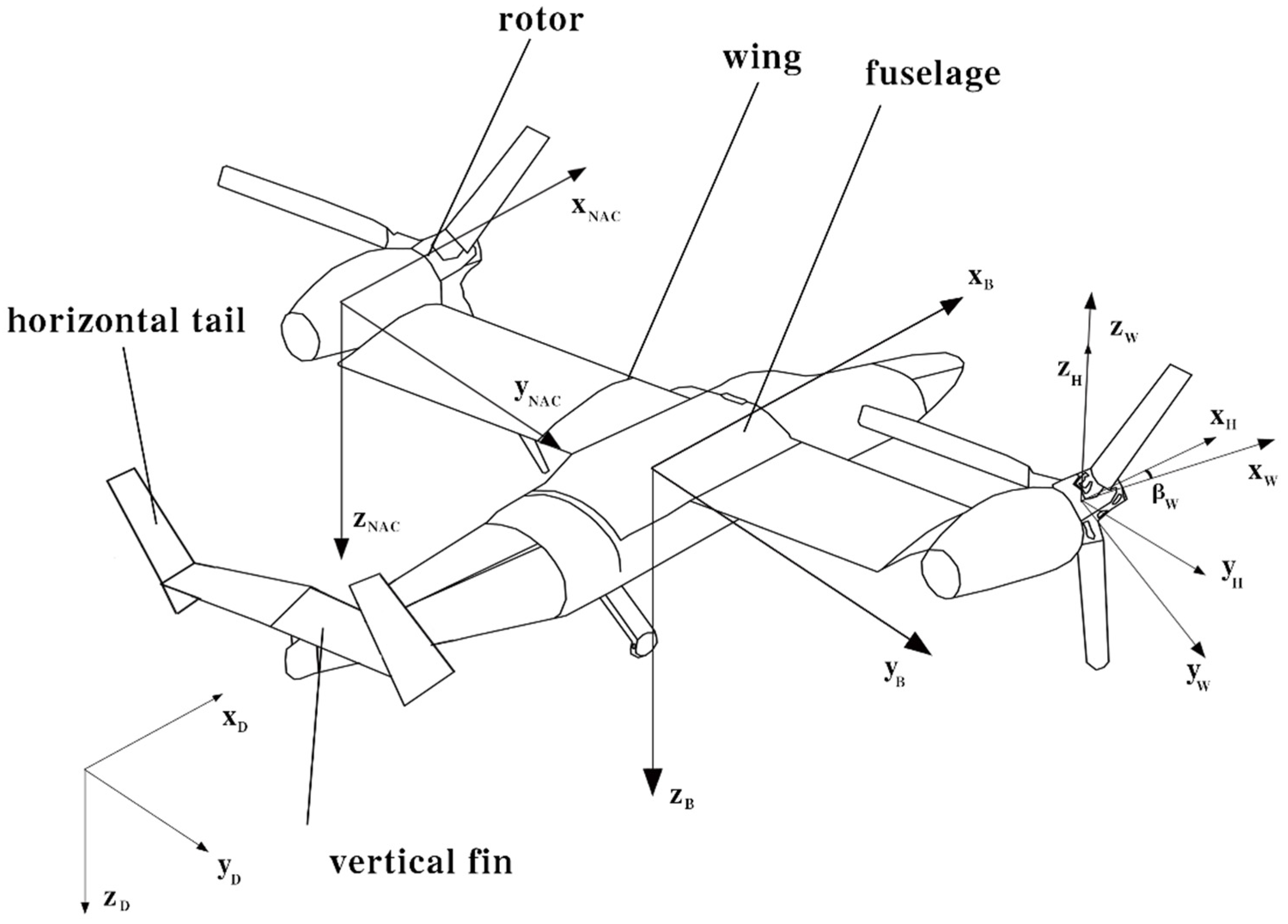
The main aerodynamic components of a tiltrotor aircraft are its rotor, wing, fuselage, horizontal tail (incl. horizontal rudder) and vertical fin (incl. vertical rudder). This paper is going to develop aerodynamic models for each component. The aerodynamic force of each component will find its solution in wind axis system and finally be converted to body axis system through the conversion matrix.
Figure 2 shows the components of the tiltrotor aircraft and the schematic diagram of some axis coordinate systems.
In order to establish an accurate flight dynamics model of tiltrotor aircraft and avoid being complex, the following basic assumptions are made in this paper
- (1)
The earth axis system is assumed to be an inertial reference system;
- (2)
Assuming that the earth is flat, the curvature of the earth is not considered;
- (3)
Tiltrotor aircraft are considered as rigid bodies;
- (4)
The rotor blades are bending rigid and linear torsion;
- (5)
The blade waving motion is calculated by taking the first-order harmonic;
- (6)
The angle of attack and sideslip angle are small angles;
- (7)
Ignore the influence of rotor downwash flow on the fuselage;
- (8)
Aerodynamic interference between left and right rotors is not considered;
- (9)
Tiltrotor aircraft is left-right symmetrical, and its longitudinal axis is its plane of symmetry.
2.1. Center of Gravity and Moment of Inertia
The center of gravity of a tiltrotor changes in its longitudinal plane as the nacelle tilts, which causes the change of the moment of inertia as well. Center-of-gravity position and moment of inertia are functions of the nacelle angle.
The nacelle angle
, center-of-gravity position is the initial position. The variation of center-of-mass position as the nacelle angle changes is expressed as:
where,
is the rotor’s height against the wing,
is the mass of the nacelle system,
is the gross weight of the airframe.
Moment of inertia changes along with the nacelle angle
change, which is formulated as [
10]:
where
is the moments of inertia of any axis in helicopter mode.
is the coefficient of the moment of corresponding inertia.
2.2. Rotor Aerodynamic Model
The rotor is the most important component of a tiltrotor. In helicopter mode, the rotor is the main lifting and control surface. In fixed-wing mode, the rotor is the propeller. While in transition mode, the rotor plays the aforesaid three roles together. That explains why it is one of the critical technologies to build a precise rotor model for a tiltrotor’s modeling.
Compared with a helicopter, a tiltrotor’s mathematical model is far more complicated thanks to the aerodynamic interferences between rotors and wings. Rotors’ downwash flow confluences at wings, and expands along wings to the fuselage, forming a “fountain flow effect”, which boosts rotors’ induced velocity. However, on the other hand, the blocking effect from wings to rotors is similar to ground effect and reduces that induced velocity. As a tiltrotor is flying at a low speed, fountain flow effect and blocking effect are generating equivalent induced velocities, which imply the aerodynamic interference from wings to rotors is negligible. Therefore, a tiltrotor can be considered equal to the aerodynamic model of an isolated rotor.
A tiltrotor is composed of left and right two rotors. They tilt in the opposite direction. The right one tilts counter-clockwise while the left one tilts clockwise. Since two rotors use the same modeling method but only differ in terms of some symbols, this paper is going to take the right rotor as an example and to build its aerodynamic model.
According to the helicopter flight dynamics theory [
20], external forces on blades in flapping plane are aerodynamic force, centrifugal force, gravity force, inertia force, etc. The resultant moment of above forces against flapping hinge is 0, that is,
.
Thus, the rotor flapping motion equation is:
where,
is the variation of center of gravity as the nacelle tilts.
The velocity being converted to the rotor hub wind axis system at the rotor hub center in the aircraft-body axis system is:
Tangential velocity and vertical velocity of the rotor profile, respectively, are:
By blade element theory, take blade element of radial position on propeller and width
, and chord
, therefore lift force and resistance force of blade element are:
Component force converted to flapping plane is:
The projection of blade element’s aerodynamics onto the rotor structure axis system constitutes the rotor’s elemental force and moment .
Integrate the above blade element elemental aerodynamic force and moment along the propeller, take its average value against position angle, and then multiply with the number of blades to get the force and moment generated by rotors: .
In calculating the rotor’s elemental force, its induced velocity cannot be calculated directly by explicit formula. This paper applies the iteration method. Given the initial value of induced velocity in the rotor’s vertical velocity, the rotor’s thrust is obtained by above equation and the new induced velocity by momentum theory is calculated as below:
Equivalent induced velocity is:
where
is inflow ratio:
,
is the rotor thrust coefficient.
If and are close enough, iteration will exit, otherwise renew with . It will work out the rotor’s induced velocity as well as its force and moment.
Convert the force and moment of the rotor into aircraft-body axis system to get its force and moment in that system:
Follow the same principle to work out the force and moment of the left rotor in aircraft-body axis system.
2.3. Wing Aerodynamic Model
Wing aerodynamic model of a tiltrotor is the most complex among all other components. In helicopter and transition modes, rotors’ downwash flow causes complicated aerodynamic interference on wings. This paper assumes wings are rigid and have no elastic distortion, and its aerodynamic center is the working point of force and moment.
A tiltrotor has a left wing and a right wing. Take the left wing as an example to work out its force and moment.
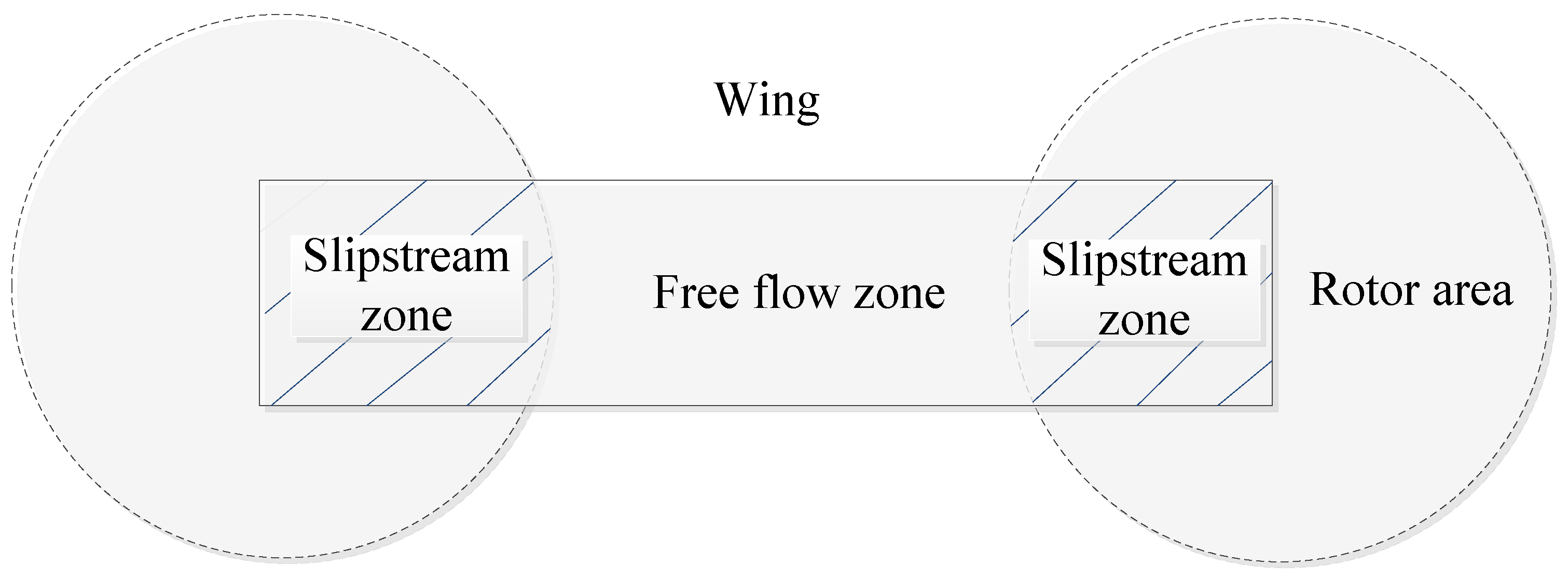
As a tiltrotor is flying at a low speed, rotors’ downwash flow confluences at wings and forms “fountain effect”. To precisely develop the wing model, the wing is divided into two parts: the first part is slipstream zone affected by rotor wake disturbance while the other part is free flow zone free from rotor disturbance. The two zones are shown as
Figure 3:
It’s hard to precisely calculate the area of slipstream zone, but the below formula can approximately estimate that area [
7]:
where,
is the maximum area of slipstream zone,
is advance ratio in helicopter mode when the wing is free from impact of rotor wake.
The area of free flow zone is the result of wing area deducting slipstream zone area.
- (1)
Force and moment in slipstream zone
In slipstream zone, the wing’s air velocity is the sum of the rotor’s induced velocity at wings and inflow ahead.
In helicopter mode, the left wing aerodynamic center has the position against the airframe center of gravity as
. As the nacelle tilts, the wing’s aerodynamic center position is:
where,
is the variation of center of gravity as the nacelle tilts.
Force and moment in the aircraft body axis system are:
- (2)
Force and moment in free flow zone
Free flow zone is dynamic. In helicopter mode, its area is the smallest. Then as the nacelle tilts, part of slipstream zone turns into free flow zone. Therefore, a free flow zone can be considered as two parts: the first part is the zone always being free flow zone (incl. wing flap), and the other part is the zone turned from slipstream zone due to nacelle tilting (incl. aileron).
In free flow zone, wing air velocity is only related to front incident flow. In calculating these two parts, aerodynamic center position deserves more attention.
First, calculate the air velocity , in the two parts free flow zone of the wing, respectively, and then calculate the aerodynamic center dynamic pressure , and angle of attack , , respectively, in the free flow zone of the left wing according to the air velocity in the free flow zone.
Then, calculate the Lift force , resistance force and moment of left wing in free flow zone are:
Aerodynamics in free flow zone in the aircraft-body axis system are:
Moment in free flow zone in the aircraft-body axis system are:
Take the sum of force and moment of the left wing in slipstream zone and free flow zone, which is the force and moment received by the left wing. Follow the same principle to get the force and moment of the right wing. The total force and moment on left and right wings are the gross sum of forces and moments of all wings.
2.4. Fuselage Aerodynamic Model
The fuselage is complex in structure and subject to aerodynamic disturbance from rotors and wings. This paper is going to neglect aerodynamic disturbance from rotors and wings and apply a simplified approach to fuselage modelling. Force and moment of the fuselage are calculated in local wind axis system, working point is the airframe aerodynamic center, which means the calculated force and moment need converted to the body axis system.
First, calculate air velocity at fuselage aerodynamic center (), and then calculate dynamic pressure , angle of attack and sideslip angle of the fuselage according to the air velocity at fuselage aerodynamic center.
Then, calculate the aerodynamic force and moment of the fuselage in wind axis system.
At the end, work out aerodynamic force and moment of the fuselage in body axis system through the conversion matrix from wind axis frame to body axis frame.
2.5. Horizontal Tail Aerodynamic Model
Rotor wake has minor impact on horizontal tail, so rotor wake will be overlooked in this paper. Calculate aerodynamic force of horizontal tail and elevator by following the way of treating a fixed-wing. Airflow of horizontal tail pressure center () is the sum of airframe linear velocity and angular velocity.
First, calculate air velocity at horizontal tail pressure center, and then calculate dynamic pressure , angle of attack and sideslip angle of the fuselage according to the air velocity at horizontal tail pressure center.
Then, calculate the lift force and resistance force of a horizontal tail in local wind axis system.
Force and torque in wind axis system are converted into body axis system:
2.6. Vertical Fin Aerodynamic Model
The vertical fin and rudder have a similar modelling method as horizontal tail. Calculate aerodynamic force and moment of vertical fin in wind axis system and then convert them to body axis system. A tiltrotor has two vertical fins, so it’s necessary to develop models for both left and right fins. This paper will take the left fin as an example.
Calculate air velocity at vertical fin aerodynamic center (), and then calculate dynamic pressure , angle of attack and sideslip angle of the fuselage according to the air velocity at vertical fin aerodynamic center.
Thus, aerodynamic force of the vertical fin in wind axis system is:
Aerodynamic force and moment converted to body axis system are:
In the same way, work out force and moment of the right vertical fin. The sum of force and moment of the right and left fins is the gross force and moment of vertical fins in aircraft-body axis system.
3. Nonlinear Simulation Modelling
The resultant external force and moment exerted on a tiltrotor is:
According to momentum theorem, we can get:
According to theorem of moment of momentum, we can get:
where
Supplementary kinematic equation group is:
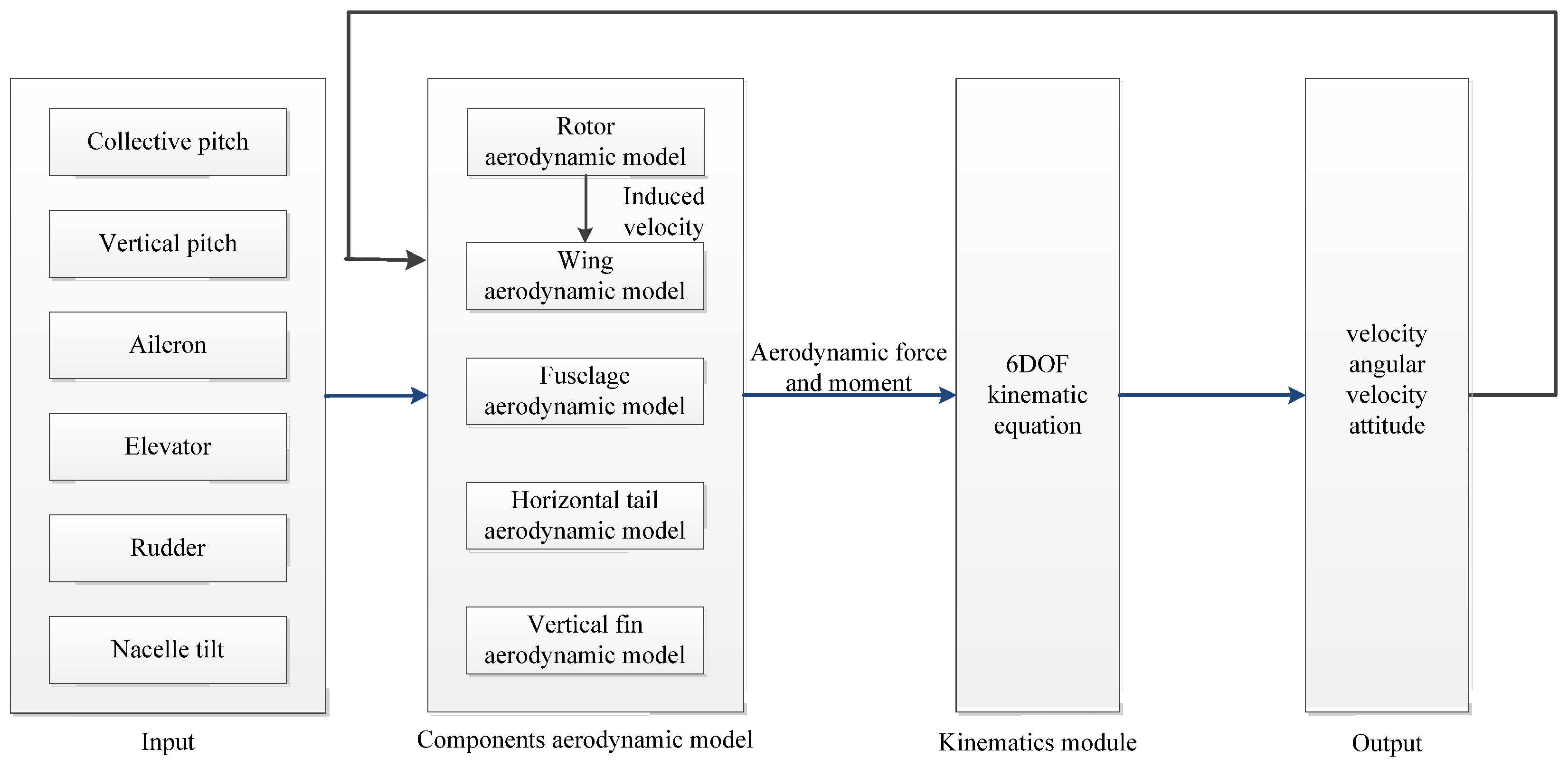
The above is a tiltrotor’s 6DOF flight dynamics equation. The above equation group, if solved, will determine the aircraft’s flight condition. This paper uses Function S of MATLAB to develop a tiltrotor’s non-linear simulation model. From
Section 1, it’s known that respective aerodynamic models for the rotor, wing, fuselage, horizontal tail and vertical fin will be developed. Substitute the calculated force and moment from each component to 6DOF flight dynamics equation, which will get us the nonlinear mathematical modelling of a tiltrotor aircraft. The model has the structure diagram as described in
Figure 4:
4. Trimming and Result Analysis
After the non-linear simulation model is built, it is necessary to validate its effectiveness and accuracy. Thus, this paper is going to compare trimming results of the built model and actual trimming results. Considering the inevitability of errors, if the change trend is aligned and values are close, it can be deduced that the built model reflects flight characteristics of a tiltrotor, which means the model built in this paper is accurate and effective.
Steady flight is the case where the aircraft’s linear and angular velocity are constant. Then all external forces and moments exerted on the aircraft are zero, the aircraft stays in state of equilibrium. The maneuver applied to reach equilibrium is called trim control. The trimming calculation is based the condition that force and moment acting on the aircraft in steady flight condition is balanced, and then use appropriate mathematical algorithms to define control inputs in trimmed condition. Mathematically speaking, trimming is the point to make sure the system status derivative as zero. The most popular trimming methods are the Newton iteration method, simplex method, steepest descent method, genetic algorithm, particle swarm optimization algorithm, etc. Meanwhile, MATLAB/Simulink toolkit also provides trim function, which also uses optimization algorithms. Thus, this paper is going to perform trimming with trim function.
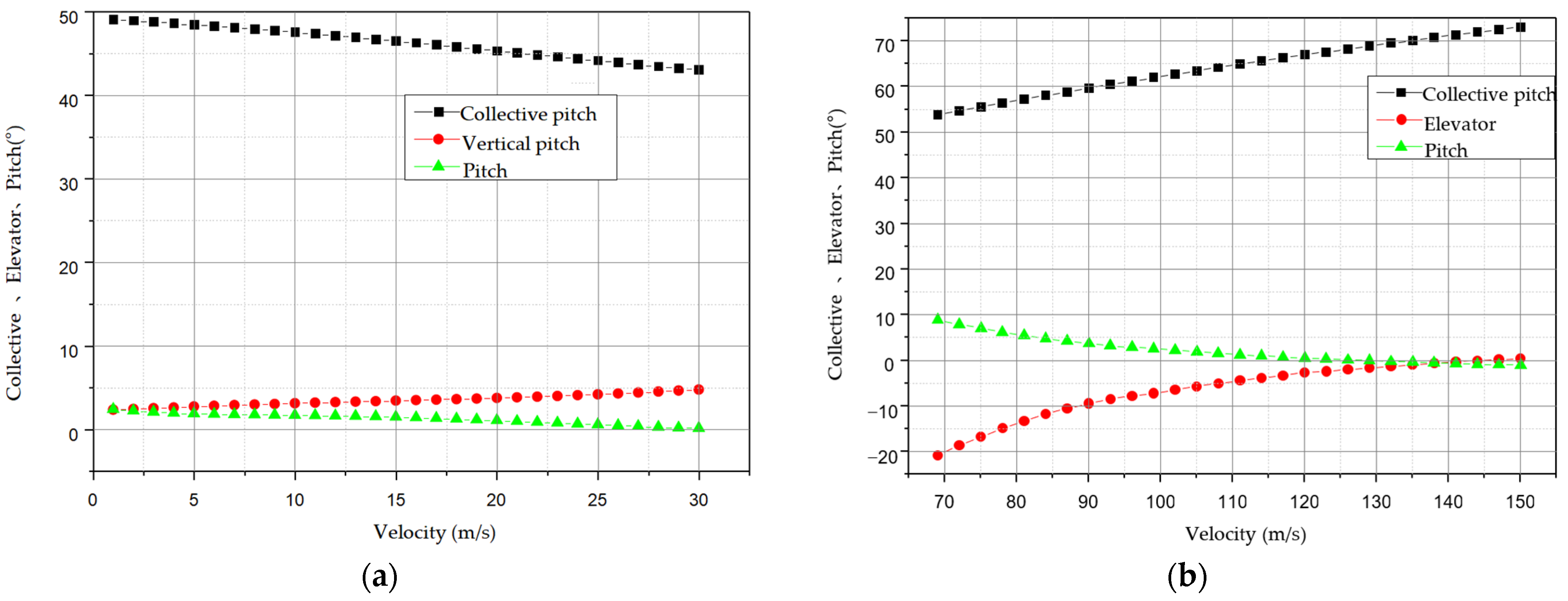
This paper takes an XV-15 tiltrotor as an example, builds its mathematical model in Simulink, and then trims it with the trim function. Trimming results in helicopter mode, flight mode and transition mode where nacelle tilt angles are 15° and 75° are given hereafter.
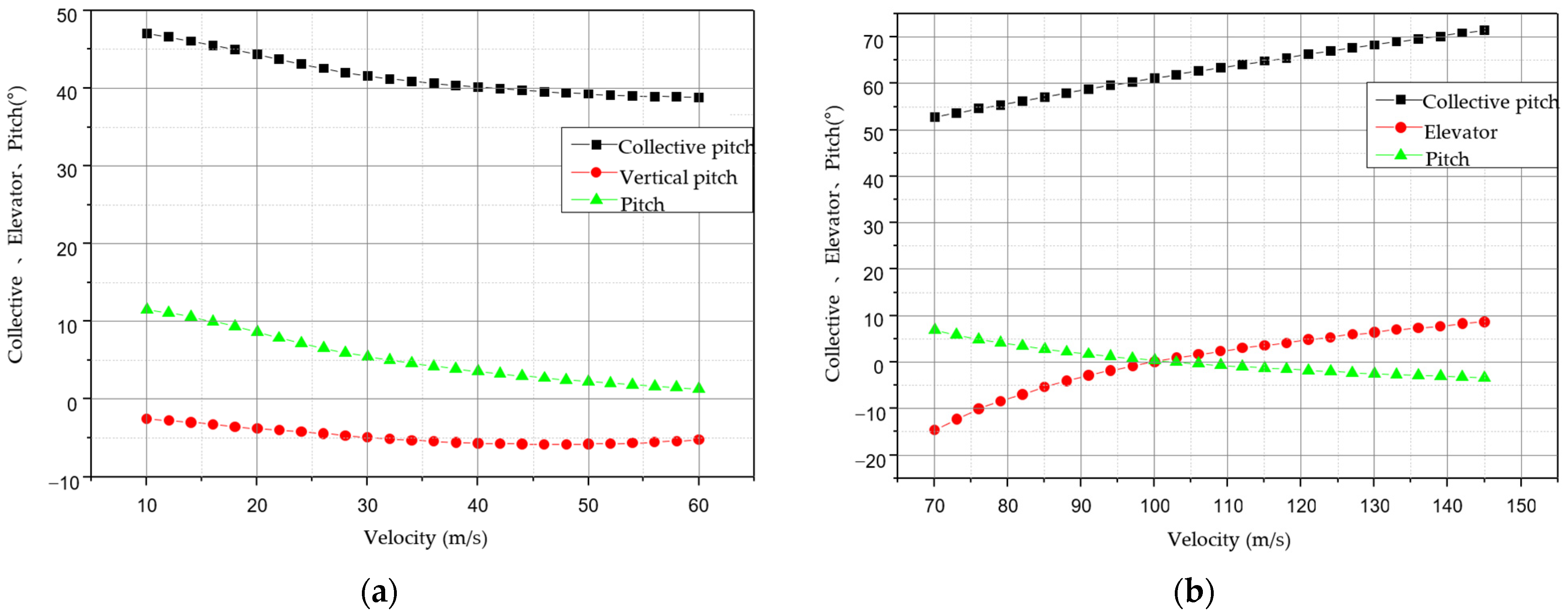
Trimming results in helicopter mode and flight mode is as
Figure 5, Trimming results at transition mode when nacelle tilt angle is 75° and 15° is as
Figure 6:
Trimming results are analyzed in below:
In helicopter mode: an aircraft starts forward flight from hovering. With the velocity increasing, disturbance from wings to rotors reduces, lift force provided by wings starts to increase, collective pitch input starts to reduce. As the aircraft flight velocity increases, a forward force is necessary to supply, thus need increase vertical pitch. The bigger the flight velocity is, the bigger vertical pitch is necessary to be supplied. At the meantime of vertical pitch increase, nose-down pitch is generated, which means the aircraft’s angle of pitch will continuously reduce.
In-flight mode: rotors are equivalent to propellers. As the flight velocity increases, resistance on the airframe and propeller plane increases. To overcome the resistance, it is necessary to increase collective pitch. While with the velocity increases, rudder effectiveness reinforces, so the rudder maneuver decreases continuously.
Transition mode: when the nacelle tilt angle is 15°, use helicopter manipulation method, compared to helicopter mode, forward flight velocity is the same and collective pitch maneuver is quite small, which is mainly caused by nacelle tilt leading to the dramatic reduction of blocking effect of wings on rotors. In the meantime, flight velocity increases and lift force provided by wings increases, so the collective pitch control keeps on reducing. Forward force generated by nacelle tilt, backward force generated by propeller plane moving backward, velocity increasing, pitch angle decreasing, more nose-down and vertical cyclic feathering reduction all together lead to a negative vertical pitch.
When the nacelle tilt angle is 75°, use fixed-wing aircraft control. Compared to aircraft mode, forward flight velocity is the same and collective pitch maneuver is quite small, which is due to the fact that the rotors have been equaled to propellers. As the nacelle angle increases, propeller plane resistance increases along, which needs a bigger collective pitch to generate thrust to obtain balance.
To test accuracy and effectiveness of the model, this paper will take flight model as an example. Given the comparison between the balancing results of the mathematical model, the GTRS results and the actual balancing results of XV-15 is given. The comparison result is as
Figure 7.
The balancing results are completely consistent in trend, which shows that the model is feasible and reasonable. However, due to the lack of the data of XV-15, there will inevitably be some differences in the results. the model does not need a lot of experimental data to look up the table, which makes the model have good universality.
5. Tiltrotor Maneuvering Stability Characteristics Analysis
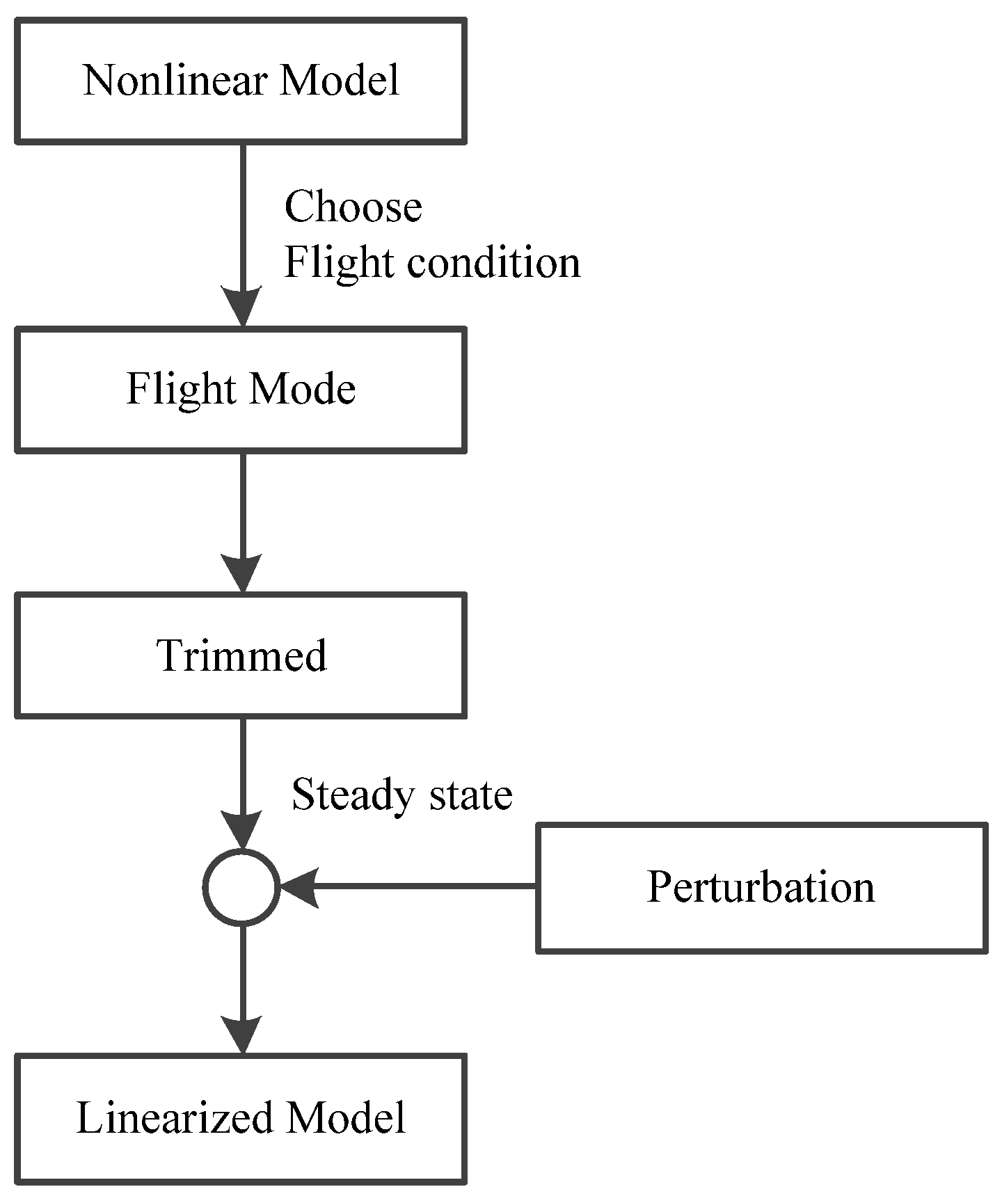
Flight dynamic linear differential equations, to simplify analysis and equation solution.
Non-linear model can be linearized by following steps as
Figure 8:
The above figure describes how to turn a non-linear model to linear model. Linear model is obtained by linearizing a steady flight condition and by trimming kinematic equations of that steady flight condition to obtain corresponding steady-state values.
Balance point is shown as Equation (37):
where,
is the trimmed value of state vector.
is the control vector in steady state.
At balance point, a small disturbance on flight kinematic equation being assumed and trimmed will get the linearized model, which is written to state space as:
where,
is state variable,
is control variable.
A and
B are matrixes of coefficients.
Where, state variable is:
In the previous section, the aircraft’s balance point is trimmed. By the function Linmod in the MATLAB/Simulink environment, one can obtain a non-linear model near the balance point linearized and obtain an A matrix and B matrix.
5.1. Helicopter Mode
5.1.1. Derivative Analysis
The parameters of matrix A and matrix B in helicopter mode are shown in
Table 1 and
Table 2. Stability derivative analysis on Matrix A is performed as below:
, : forward flight speed increases, rotors flap backward, rotor thrust vector is backward, which results in as negative. At the meantime, upward thrust of wings and horizontal tail increases, as negative.
, :: being small explains that disturbance of vertical speed has little impact on force in X direction. Increase of will enlarge the rotor’s angle of attack, thrust of rotor increases, thus is positive and is negative.
, : as an airframe has pitching movement, passive flapping will happen, decreases, thus and are positive.
, : increase leads to the rotor’s angle of attack and thrust of rotor increasing, thus is negative. And, analogous to instability of helicopter angle of attack, rotors reverse backward, is negative.
, and : forward flight speed increases, rotor tip plane is reversing, backward force increases, pitch-up moment is generated, is positive. being zero is since the vertical distance from the rotor hub to the aircraft center is short, moment change is small. As analyzed afore, as there is pitching movement, passive flapping happens, the increased force in X and Y directions leads to nose-down moment, and thus is negative.
5.1.2. Eigenvalue Analysis
Eigenvalue is a very important characteristic of analyzing stability of the model. It demonstrates a vehicle’s motion modes under different flight conditions. Since longitudinal and lateral coupling of a helicopter is severe, for easier analysis, this paper is going to discuss longitudinal module and lateral module in helicopter mode separately.
By observing eigenvalues as
Table 3, it can be found that a tiltrotor’s right half plane in helicopter mode has roots, which means its stability in such mode is poor and control system must be applied to improve stability.
Longitudinal eigenvalue: motion modes of velocity and angle of attack corresponding to a pair of positive complex conjugate roots are similar, with long period and divergent. Motion modes of angle of attack and angle of pitch corresponding to a pair of negative complex conjugate roots converge fast.
Lateral eigenvalue: the mode of complex conjugate roots is similar to the oscillation mode of longitudinal hovering. Large negative real root corresponds to rolling convergence mode. Since rotors rotate behind the airframe, rotors have larger rolling aerodynamic damping and converge faster. Small negative root represents spiral mode. Zero root means level flight in any heading course has no difference.
5.2. Flight Mode
5.2.1. Derivative Analysis
The parameters of matrix A and matrix B in flight mode are shown in
Table 4 and
Table 5. Stability derivative analysis on Matrix A is performed as below:
, : forward flight speed increases, airframe resistance and propeller resistance increase, and thrust generated by wings increase, which leads to as negative. Thrusts of wings and horizontal tail increase, as negative.
, : increases, vertical upward air flow increases, angle of attack of wings increases, lift component in X direction increases, so is positive. increase leads to the increase of thrust of wings, is negative.
, : increase, downward airflow at wings is generated, thrust of wings reduces, is positive. Backward thrust component of wings increases, is negative.
, : increase, thrust vector of wings is backward, is negative. Since the aircraft has pitch-up already, with the increase of , it pitches up more. Thrust is reducing in Z direction, is negative.
, and : increase, airframe resistance and propeller resistance increase, which leads to the tiltrotor pitching up, is positive. increase, thrust of wings is forwarding, pitching-up moment reduces, is negative. increases, significant upward airflow at horizontal tail is generated, thrust of horizontal tail in Z direction increases, which leads to bigger nose-down moment, and is negative.
5.2.2. Eigenvalue Analysis
Eigenvalues in flight mode is shown as
Table 6. Different from the helicopter mode, the flight mode has less severe longitudinal and lateral coupling than that in helicopter mode and thus has much better stability. Eigenvalue analysis at forward speed of 100 m/s in flight mode is performed.
Longitudinal eigenvalue: the longitudinal mode has long period and short period (two modes). The external force generated after receiving disturbance makes it hard to change flight speed but easy to change the angle of attack (incl. angle of pitch). The long period mode corresponds to speed mode while the short period mode corresponds to the angle of attack variation.
Lateral motion: large complex roots represent rolling convergence mode, since wings converge quickly for large aerodynamic damping. Small complex roots correspond to the spiral mode. A pair of complex conjugate roots represent oscillating motion mode, also known as Dutch roll mode, a motion mode in which heading course and rolling are recurrent.
6. Conclusions
This paper adopts the dividing modeling method, which breaks down a tiltrotor into five parts, rotor, wing, fuselage, horizontal tail and vertical fin, develops aerodynamic models for each part and thus obtains force and moment generated by each part. The force and moment then is converted to the airframe coordinate frame. By blade element theory, the rotor’s dynamic model and rotor flapping angle expression are built. Then, according to mature lifting line theory, dynamic models of the wing, horizontal tail, and vertical fin are built. At the meantime, the rotor’s dynamic interference on wings and nacelle tilt’s variance against center of gravity and moment of inertia are considered. A more perfect mathematical model of the tilt rotor aircraft is established.
In the MATLAB/Simulink simulation environment, a non-linear tiltrotor simulation model is built, Trim command is applied to trim the tiltrotor and an XV-15 tiltrotor is taken as an example to validate accuracy and rationality of the model developed. Due to the lack of complete XV-15 data, there will inevitably be some differences in the results. The results show that the trend of the model is completely consistent with the actual data and GTRS model, which validate the accuracy and rationality of the model developed.
In the end, the non-linear simulation model is linearized to get State-space matrix, the stability derivative and eigenvalue of the tiltrotor are analyzed, and furthermore the tiltrotor’s stability in each flight mode is studied. The stability of the aircraft in the helicopter mode is poor, which must be improved through the control system. The vertical and horizontal coupling of the flight mode is not as serious as that of the helicopter mode, and the stability is much better than that of the helicopter mode. It therefore provides a theoretical basis for the subsequent controller setting.


