Article

Long Distance Ground Target Tracking with Aerial Image-to-Position Conversion and Improved Track Association

School of AI, Daegu University, Gyeongsan 38453, Korea
Drones 2022, 6(3), 55; https://doi.org/10.3390/drones6030055
Submission received: 7 February 2022 / Revised: 22 February 2022 / Accepted: 22 February 2022 / Published: 23 February 2022
(This article belongs to the Special Issue Feature Papers of Drones)

Abstract

:
A small drone is capable of capturing distant objects at a low cost. In this paper, long distance (up to 1 km) ground target tracking with a small drone is addressed for oblique aerial images, and two novel approaches are developed. First, the coordinates of the image are converted to real-world based on the angular field of view, tilt angle, and altitude of the camera. Through the image-to-position conversion, the threshold of the actual object size and the center position of the detected object in real-world coordinates are obtained. Second, the track-to-track association is improved by adopting the nearest neighbor association rule to select the fittest track among multiple tracks in a dense track environment. Moving object detection consists of frame-to-frame subtraction and thresholding, morphological operation, and false alarm removal based on object size and shape properties. Tracks are initialized by differencing between the two nearest points in consecutive frames. The measurement statistically nearest to the state prediction updates the target’s state. With the improved track-to-track association, the fittest track is selected in the track validation region, and the direction of the displacement vector and velocity vectors of the two tracks are tested with an angular threshold. In the experiment, a drone hovered at an altitude of 400 m capturing video for about 10 s. The camera was tilted 30° downward from the horizontal. Total track life (TTL) and mean track life (MTL) were obtained for 86 targets within approximately 1 km of the drone. The interacting multiple mode (IMM)-CV and IMM-CA schemes were adopted with varying angular thresholds. The average TTL and MTL were obtained as 84.9–91.0% and 65.6–78.2%, respectively. The number of missing targets was 3–5; the average TTL and MTL were 89.2–94.3% and 69.7–81.0% excluding the missing targets.

1. Introduction

Small unmanned aerial vehicles (UAVs), or drones, are useful for security and surveillance [1,2]. One important task is to track moving vehicles with aerial video. A small drone captures video from a distance at a low cost [3]. No highly trained personnel are required to generate the video.
Ground targets can be tracked with a small drone with visual, nonvisual, or combined methods. Various deep learning methods with camera motion models were studied in [4]. Tracking performance can be degraded by small objects, large numbers of targets, and camera motion [5]. Deep learning-based object detection was combined with multi-object tracking and 3D localization in [6]. In [7], YOLO and Kalman filter were used to detect and track high-resolution objects. The object detector and tracker with deep learning may require heavy computation with massive training data [8,9].
The background subtraction and the adaptive mean-shift and optical flow tracking were developed for the video sequences captured by a drone in [10]. The mean-shift tracker based on particle filtering was utilized to track a small and fast-moving object in [11]. The SIFT feature-based tracker was developed for fast processing in [12]. The kernelized correlation filter-based target tracking was studied in [13]. In [14], object tracking was performed by handing over the camera from one drone to another. Ground targets were tracked with road geometry recovery in [15]. Usually, trackers based on video sequences transmit high-resolution video streams to the ground, or a high computational burden is imposed on the drone. Aerial video was processed with high-precision GPS data from vehicles in [16]. Bayesian fusion of vision and radio frequency sensors were studied for ground target tracking in [17]. In [18], computer vision-based airborne target tracking with GPS signals was studied. Object tracking from drones with nonvisible cameras can be found in literature. A boat was captured and tracked with the Kalman filter by a fixed-wing drone in [19]. A small vessel was tracked by adopting a colored-noise measurement model in [20]. In the nonvisual approach, high-cost sensors add more payload to the drone, or infrastructure is required on the ground or in a vehicle.
In this paper, moving vehicle tracking with a small drone at long distances (up to 1 km) is addressed. In the previous work [21,22,23,24], the drone’s camera was pointed directly at the ground, or the altitude of the drone was very low. When the camera is tilted, the field of view (FOV) can be extended, but constant scaling from pixel coordinates to actual position can no longer be applied. Therefore, an image-to-position conversion is developed to change the integer coordinates of a pixel to its actual positions, assuming that the angular field of view (AFOV), tilt angle, and camera (drone) altitude are known.
Moving object detection consists of frame subtraction and thresholding, morphological operation, and false alarm removal; falsely detected objects are removed using the object’s actual size and two shape properties: squareness and rectangularity [23,24]. The minimum size of the extracted object is set constant, but the converted value in pixels changes depending on the distance from the drone.
Target tracking consists of three stages: track initialization, track maintenance, and track termination. Tracks are initialized with the difference between the two nearest measurements in consecutive frames following speed gating. Tracks are maintained by state estimation, measurement-to-track association (abbreviated as measurement association), and track-to-track association (abbreviated as track association). The nearest neighbor (NN) measurement association updates the state of a target by combining the measurements that are statistically closest to the prediction. The interacting multiple model (IMM) filters with a constant velocity (CV) or constant acceleration (CA) motion models are adopted to handle the various maneuvers of the target [25,26]. Track association fuses multiple tracks into a single track [27]. In this paper, the track association scheme is improved to fuse multiple tracks by sequentially searching for the nearest track in a dense track environment. Figure 1 shows a schematic block diagram of object detection and target tracking by a small drone at a long distance. First there is the image-to-position conversion, and finally there is the reverse process, position-to-image conversion.
In the experiment, the drone hovered from a fixed position at a height of 400 m. The title angle was 60° producing video for 10 s. Figure 2 shows three sample scenes extracted from a sample frame. The extracted area is 100 × 60 pixels and shows 2–3 vehicles with different resolutions. Overall, the frame has low resolution, and the targets are sometimes occluded by trees, structures, and other cars. Road lanes, traffic signs, and shadows can be included in backgrounds. A total of 86 targets within approximately 1 km of the drone were investigated with total track life (TTL) and mean track life (MTL). The average TTL and MTL were obtained as 84.9–91.0% and 65.6–78.2%, respectively, by various angular thresholds for directional track association. The number of missing targets was 3–5; the average TTL and MTL were 89.2–94.3% and 69.7–81.0%, respectively, if the missing targets are excluded.
The rest of the paper is organized as follows: the image-to-position conversion is described in Section 2. Section 3 explains multiple target tracking. Section 4 details the improved track association. Section 5 presents the experimental results. Discussion and conclusions follow in Section 6 and Section 7, respectively.

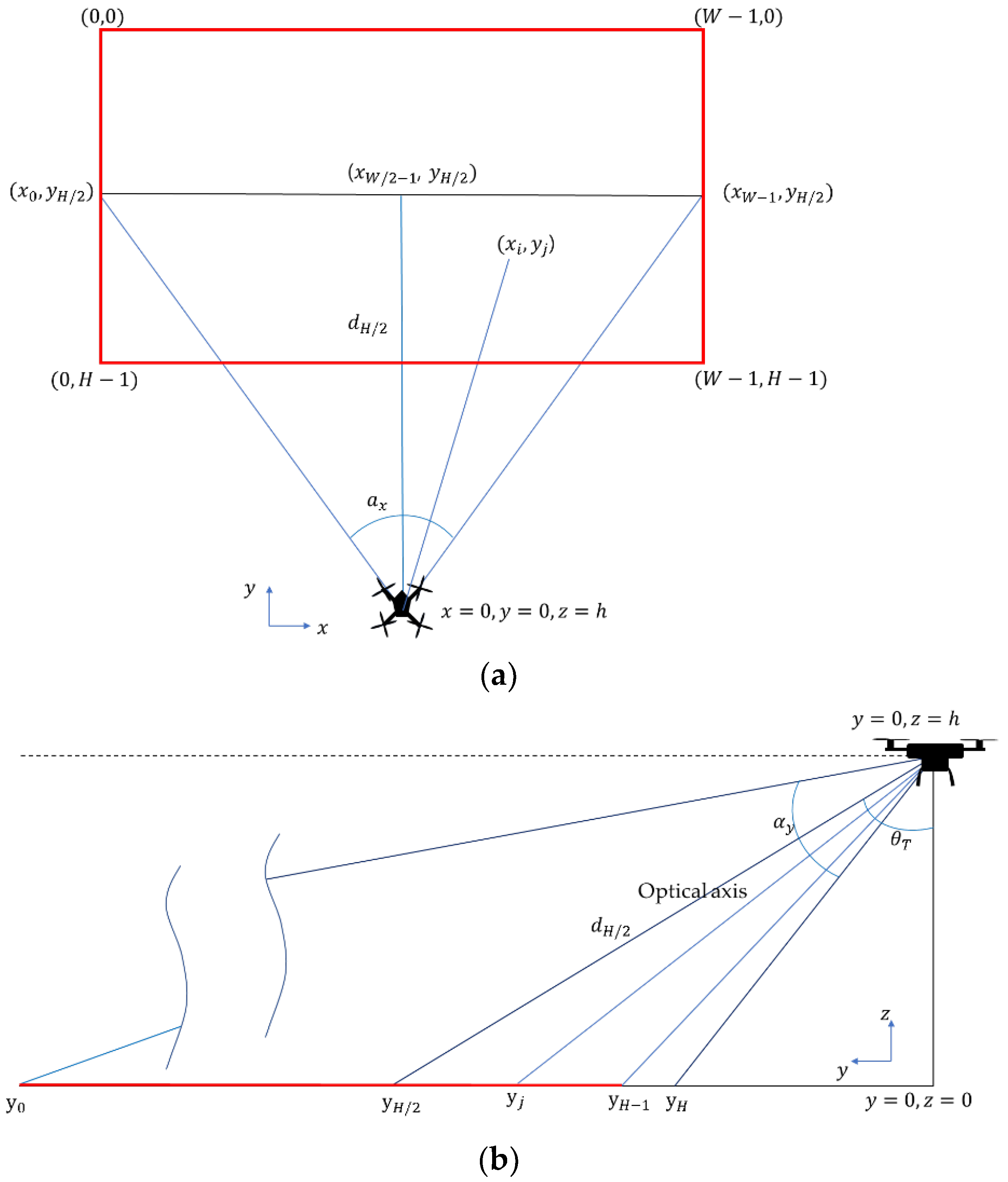
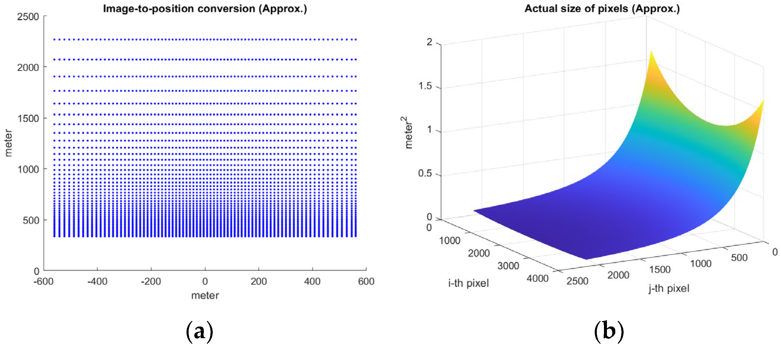
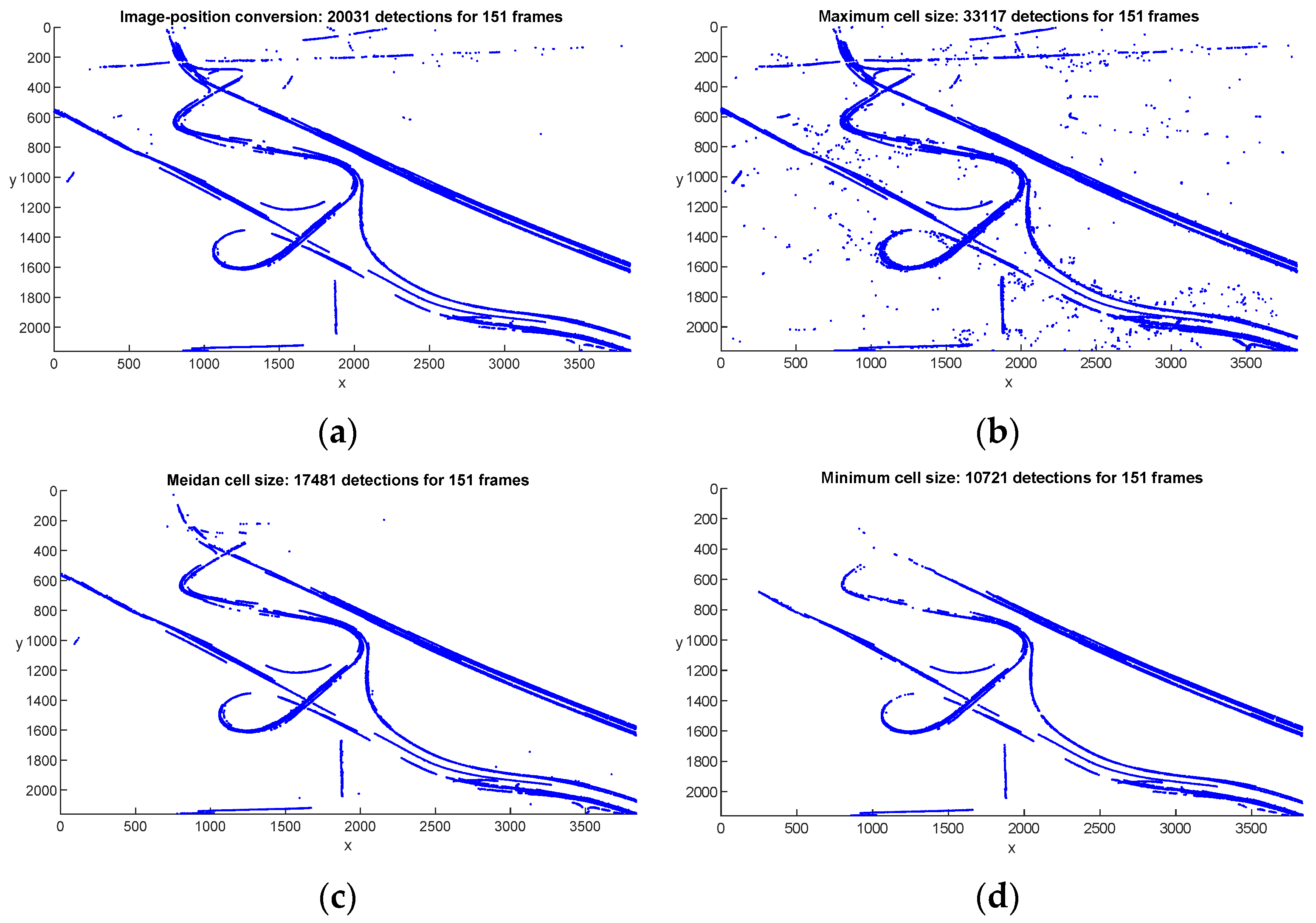
2. Image-Position Conversion

Imaging is the projection of a three-dimensional real-world onto a two-dimensional plan. Thus, when the camera is not pointed directly at the ground, the discrepancy between the relative pixel positions in the image and the real world becomes irregular. Since the coordinates of the image are not indexed in proportion to the actual distance, constant scaling generates more discrepancy between the coordinates in the image and the coordinates in the real world. Therefore, integer coordinates in x and y directions of the image are converted to real-world positions based on the AFOV, tilt angle, and altitude of the camera. As shown in Figure 3, the drone camera is positioned at (0,0,h) with a tilt angle θT. The image size is W × H pixels. The actual position vector x i j of the (i, j) pixel is approximated as
x i j = ( x i ,   y j ) ( d H 2 · tan [ ( i W 2 + 1 ) a x W ] ,    h   · tan [ θ T + ( H 2 j ) a y H ] ) , i = 0 , , W 1 ,   j = 0 , , H 1 ,
where a x and a y are the view angles of the camera in x and y directions, respectively; d H / 2 is the distance from the camera to ( x W / 2 1 , y H / 2 ,0), which is   y H / 2 2 + h 2 . It is noted that land is assumed to be flat. Thus, the position in z direction is zero. The actual pixel size is calculated as
Δ ( i , j ) = | ( x i x i + 1 ) · ( y i y j + 1 ) | .
In the experiments, the altitude h is set to 400 m; W and H are 3840 and 2160 pixels; a x and a y are set to AFOV of the camera, 70° and 40°, respectively; θ T is set to 60°; thus y H / 2 is calculated at 692.8 m by Equation (1), and d H / 2 is 800 m accordingly.
Figure 4 provides the visualization of the coordinate conversion and actual pixel size according to Equations (1) and (2), respectively. In Figure 4a, every 50th pixel is shown for better visualization. The maximum, median, and minimum pixel sizes in Figure 4b are 1.623 m2, 0.1506 m2, and 0.0561 m2, respectively. This approximate conversion considers x and y directions separately. Thus, a simple reverse process is possible from position to image, and it will be shown that the detection result is significantly improved in the experiments although the coordinate conversion can be accompanied by various inevitable errors [28,29].

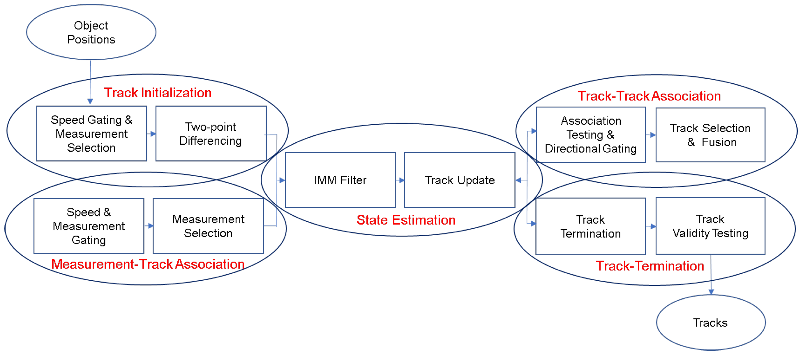
3. Multiple Target Tracking

A block diagram of multiple target tracking is shown in Figure 5.
Tracks are initialized with two-point differencing between the nearest neighbor measurements following maximum speed gating. For the measurement association, the speed gating process is first performed, followed by the measurement gating based on a chi-square hypothesis test. Then, the NN measurement selection follows. The NN rule is very effective in computing and was successfully applied to multiple ground target tracking by a drone [21,22,23,24]. The IMM filter is adopted to estimate the kinematic state of the target. It can efficiently handle various maneuvers on multiple targets. The IMM with a combined CV and CA scheme was contrived to track a single target in [24]. The IMM-CV scheme was applied to track various maneuvering 120 aerial targets for the aerial early warning system in [30]. The motion models are analyzed in detail in [31].
In a multisensor environment, a track fusion method was developed assuming the target is undergoing a common process noise [27]. A practical approach for track association was developed for the Kalman filter in [22]. This approach has been extended with the IMM filter and the directional track association was proposed to consider the moving direction of the target in [24]; directional gating tests the maximum deviation in the directions of the tracks and the direction of the displacement vector between the tracks. In this paper, the NN track selection scheme is proposed and will be described in the next section.
There are three criteria for track termination in this paper. One is associated but not selected during the track association. The other cases are the maximum frame number without measurements and the minimum target speed. The criterion of the minimum target speed is very effective when high clutter occurs on nonmoving false targets [23]. After track termination, its validity is tested with the track life length. If the track life length is shorter than the minimum track life length, the track is removed as a false track. More detailed processes of target tracking are described in [22,23,24].

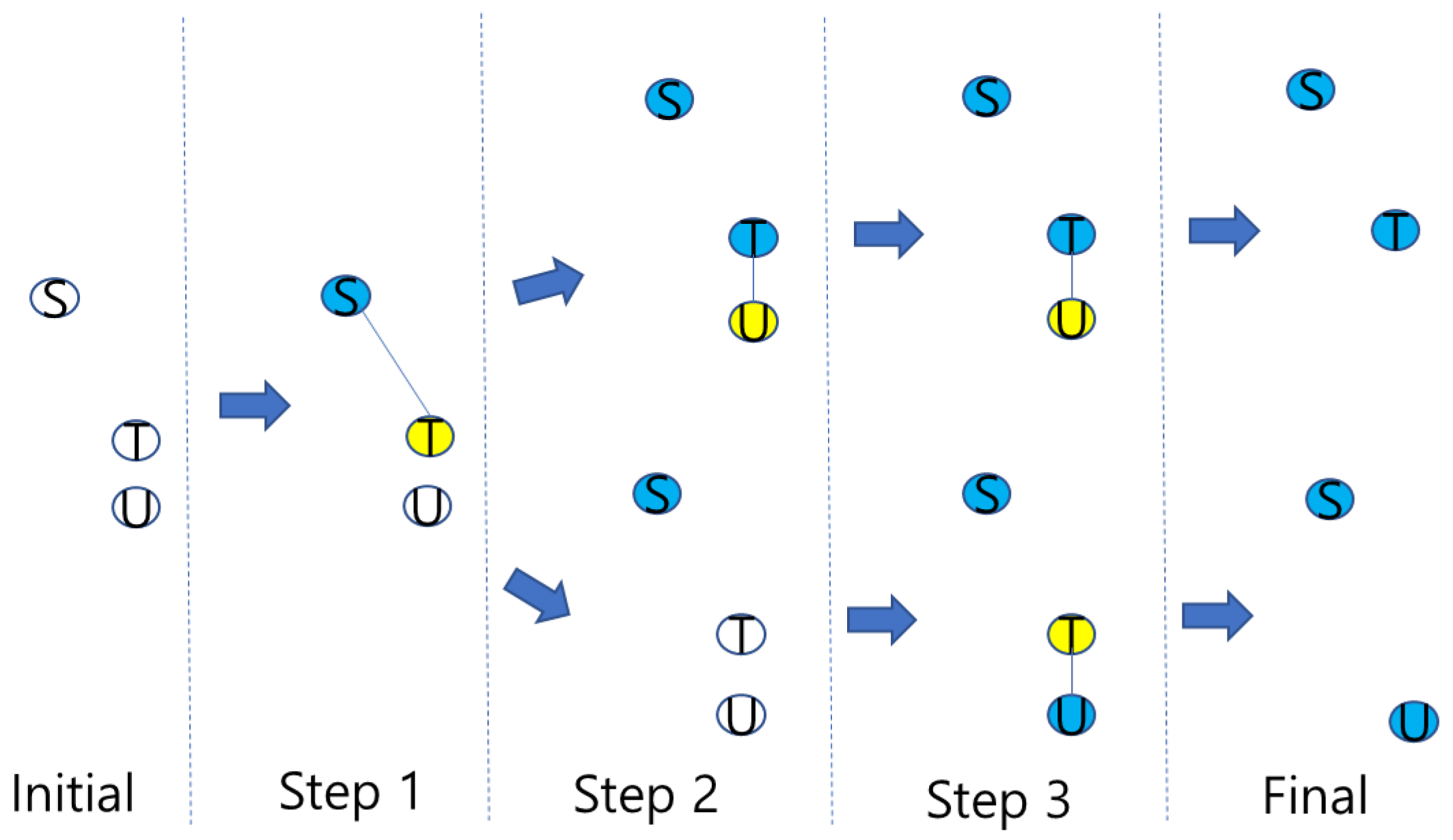
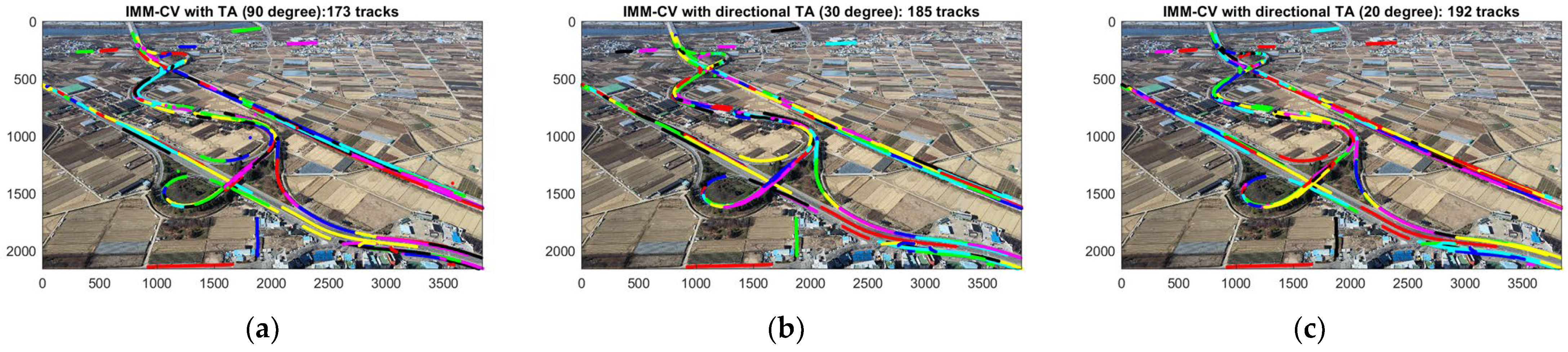
4. Improved Track Association

In this paper, the track association procedure is developed to select the fittest track in a dense track environment. For track s, the fittest track is selected as follows:
c ^ ( s ) = a r g m i n t = 1 , , N T ( k ) ,   s t [ x ^ s ( k | k ) x ^ t ( k | k ) ] T [ T s t ( k ) ] 1 [ x ^ s ( k | k ) x ^ t ( k | k ) ] ,                                 s = 1 , , N T ( k ) ,
T s t ( k ) = P s ( k | k ) + P t ( k | k ) P s t ( k | k ) P t s ( k | k )
P s t ( k | k ) = [ I b s ( k ) W s ( k ) H ] [ F P s t ( k 1 | k 1 ) F T + Q ] [ I b t ( k ) W t ( k ) H ] ,
where x ^ s ( k | k ) and x ^ t ( k | k ) are the state vector of tracks s and t, respectively, at frame k, NT(k) is the number of tracks at frame k, P s ( k | k ) and P t ( k | k ) are the covariance matrix of tracks s and t, respectively, at frame k,  b s ( k ) and b t ( k ) are binary numbers that become one when track s or t is associated with a measurement, otherwise they are zero [27]. F, H, and Q are the transition matrix, measurement matrix and covariance of the process noise, respectively. It is noted that T s t ( k ) is meaningless if its determinant is not positive. The fused covariance in Equation (5) is a linear recursion and its initial condition is set at P s t ( 0 | 0 ) = [ 0 ] N x × N x , N x is the dimension of the state vector, which is 4 and 6 for the CV and CA motion models, respectively, and W t ( k | k ) is obtained as the combined filter gain of track t as [24]:
W t ( k | k ) = j = 1 M W j t ( k | k ) μ j t ( k ) .
where M is the number of modes of the IMM filter; W j t ( k | k ) is the filter gain of the j-th mode matched filter at frame k; and μ j t ( k ) is the mode probability of the j-th mode- matched filter at frame k. The following chi-square hypothesis test should be satisfied between tracks s and t since multiple tracks of the same target have error dependencies on each other [27]:
[ x ^ s ( k | k ) x ^ t ( k | k ) ] T [ T s t ( k ) ] 1 [ x ^ s ( k | k ) x ^ t ( k | k ) ] γ g ,
where γ g is a gate threshold for the track validation region. The directional gating process tests the maximum deviation in the direction of the displacement vector and the directions of the track velocity as [24]:
m a x ( cos 1 | d ^ s t ( k | k ) ,   v ^ s ( k | k ) | d ^ s t ( k | k ) v ^ s ( k | k ) ,   cos 1 | d ^ s t ( k | k ) ,   v ^ t ( k | k ) | d ^ s t ( k | k ) v ^ t ( k | k )   ) θ g ,
d ^ s t ( k | k ) = [ x ^ t ( k | k ) x ^ s ( k | k ) y ^ t ( k | k ) y ^ s ( k | k ) ] ,   v ^ s ( k | k ) = [ v ^ s x ( k | k ) v ^ s y ( k | k ) ] ,    v ^ t ( k | k ) = [ v ^ t x ( k | k ) v ^ t y ( k | k ) ] ,
where · denotes the inner product operation, θ g is an angular threshold; and x ^ t ( k | k ) and y ^ t ( k | k ) are the position components of x ^ t ( k | k ) in x and y directions, respectively;     v ^ t x ( k | k ) and v ^ t y ( k | k ) are the velocity components of x ^ t ( k | k ) in x and y directions, respectively.
After the fittest track is selected, the current state of track s is replaced with a fused estimate and covariance if | P s ( k | k ) | | P c ^ ( s ) ( k | k ) | as
x ^ s ( k | k ) = x ^ s ( k | k )                              + [ P s ( k | k )                              P s t ( k | k ) ] [ P s ( k | k ) + P t ( k | k ) P s t ( k | k )                               P t s ( k | k ) ] 1 [ x ^ t ( k | k ) x ^ s ( k | k ) ] ,
P s ( k | k ) = P s ( k | k )                              [ P s ( k | k )                              P s t ( k | k ) ] [ P s ( k | k ) + P t ( k | k ) P s t ( k | k )                               P t s ( k | k ) ] 1 [ P s ( k | k ) P t s ( k | k ) ] .
The track selection process proposed in this paper is as follows: after track s becomes a fused track, track c ^ ( s ) becomes a potentially terminated track. That is, fusion only occurs if the determinant of the covariance matrix of track s is less than the determinant of the selected track. It is noted that a more accurate track has less error (covariance). In the previous directional track association, track c ^ ( s ) was instantly terminated, but in the procedure proposed in this paper, it is still eligible to be associated with other tracks that have not yet been fused. The detailed procedure of the track association is illustrated in Figure 6.
In Figure 6, there are initially three tracks, s, t, and u, at a certain frame. In step 1, Track s searches for the fittest track for itself. Once track t is satisfied with Equations (3), (7), (8), and | P s ( k | k ) | | P t ( k | k ) | , tracks s and t are fused, track s becomes the fused track, and track t becomes the potentially terminated track. Otherwise, no change occurs, and we go to the next step. In Step 2, track t searches for the fittest track, except for any already fused track, here track s. If track t becomes the fused track after fusion with track u, then track u becomes the potentially terminated track and is terminated at the final stage because no tracks remain to be considered for track u. Otherwise, in Step 3, track u searches and can be fused with track t. Finally, all potentially terminated tracks are terminated. In the above row, tracks s and t and tracks t and u are fused, and track u is terminated. In the bottom row, tracks s and t and tracks u and t are fused, and track t is terminated. In the next frame, the remaining tracks s and t or tracks s and u can be fused if they originate from a single target. This track association procedure allows multiple fusions of one track, and fusion occurs at most once for a track in a frame. It will be shown that it can reduce the number of tracks significantly in the experiments.

5. Results

In this section, experimental results will be detailed through video description, parameter setting, and moving vehicle tracking along with the proposed strategy.

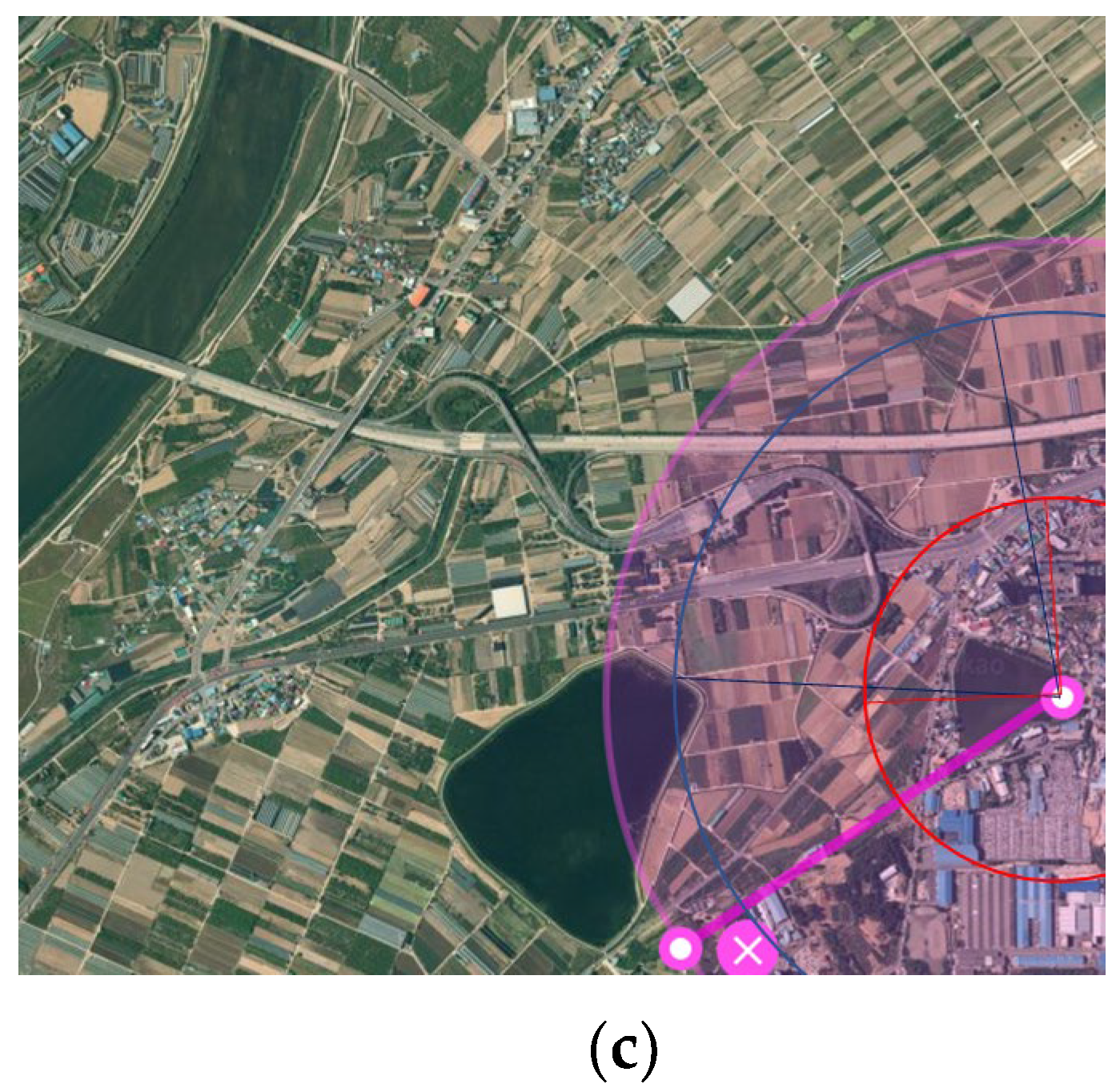
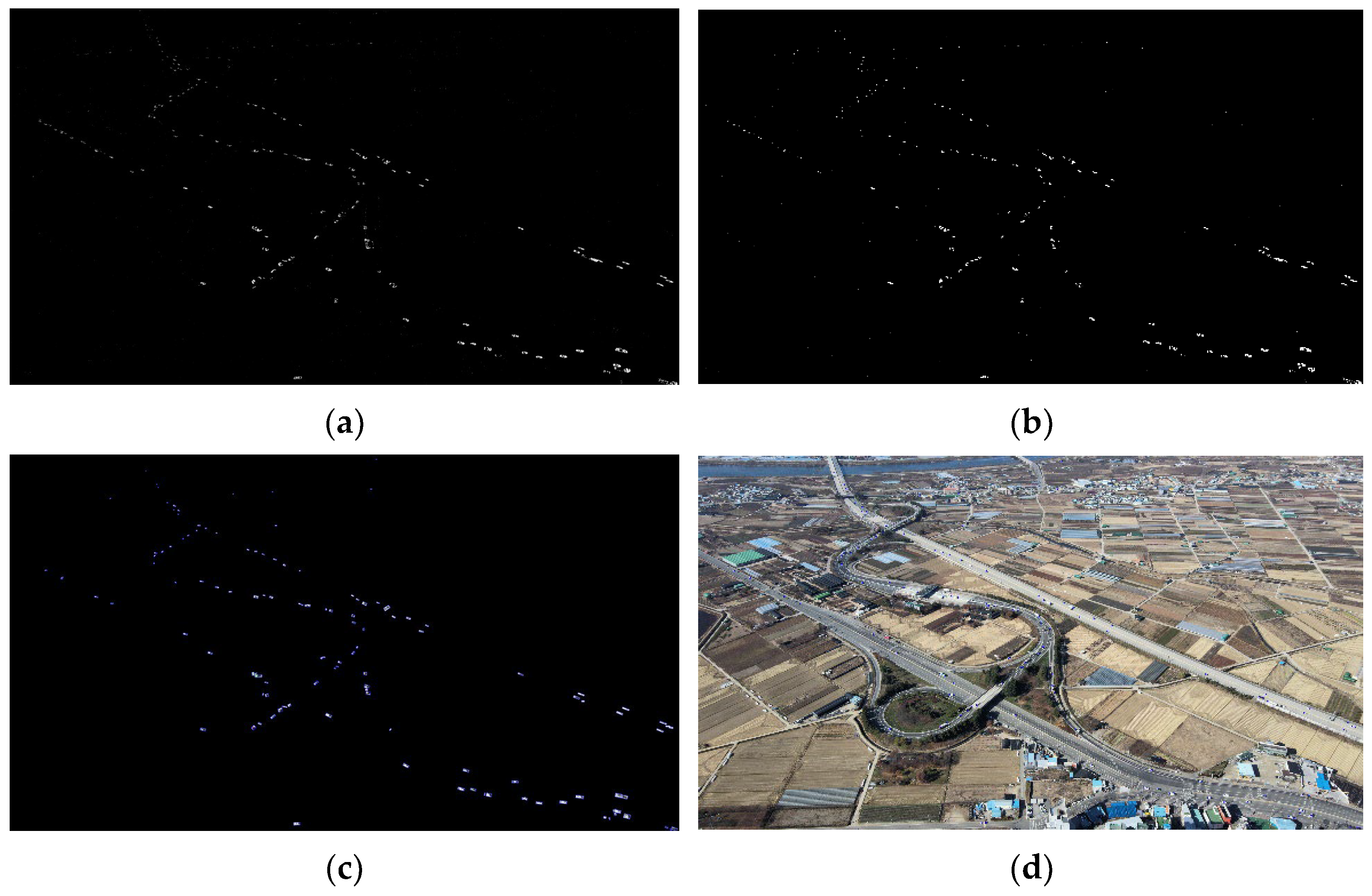
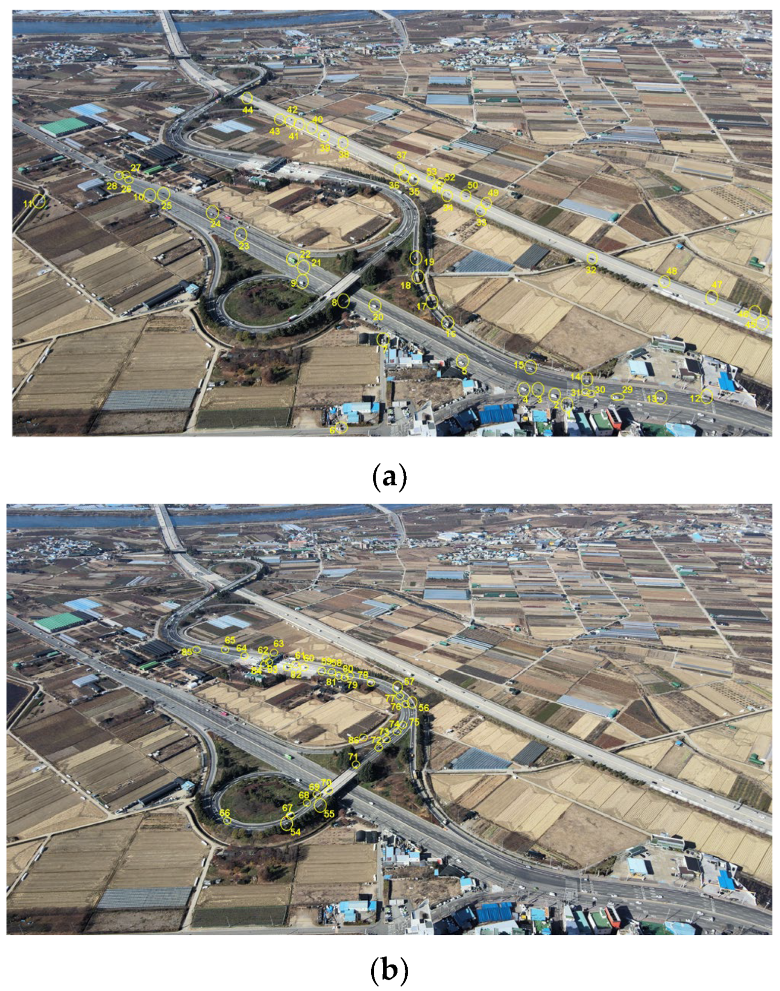
5.1. Video Description and Moving Object Detection

A video was captured by a Mavic Air 2 hovering from a fixed position at a frame rate of 30 fps. The frame size is 3840 × 2160 pixels. The scenes in the video include a highway interchange, a toll gate, road bridges, buildings, and trees. The drone was at an altitude of 400 m and the tilt angle was set to 60°. Every second, frames were processed for efficient processing, thus the actual frame rate was 15 fps. A total of 152 frames were considered for about 10 s. A total of 86 moving vehicles within a range of approximately 1 m of the drone appear in the entire video. The number of frames subtracted was 151, and the life length of the target over the entire period was 150 frames due to the two-point differencing initialization. However, the life lengths of Targets 5, 8, 29–32, 54, 62, 83, and 84 in the video are 92, 124, 42, 68,104, 100, 146, 146, 136, and 100 frames, respectively because they started late or stopped early. Some targets are occasionally occluded by a bridge, a toll gate, tress, and other vehicles. Some of them happen to be invisible because of shadows. The minimum target speed was set to 1 km/s. Thus, very slow targets were not considered as targets of interest. Figure 7a shows Targets 1–53, and Figure 7b shows Targets 54–86 in the first frame. Figure 7c shows the 1 km range with an outer circle and the view angles with blue and red lines and arcs according to distance. It is noted that Figure 7c was obtained manually to show the approximate coverage on a commercially available aerial map [32].
For the object detection, the thresholding after the frame subtraction was set to 30. The structure element for the morphological operation (closing) was set at [ 1 ] 2 × 2 . The minimum size of a basic rectangle for false alarm removal was set to 6 m2, and the minimum squareness and rectangularity were set to 0.2 and 0.3, respectively. Figure 8a is a thresholded binary image after frame subtraction between Figure 7a and the next frame.
Figure 8b is the result of the morphological operation of Figure 8a. Figure 8c is basic rectangles of Figure 8b after removing false alarms. Figure 8d shows the center of the basic rectangles, indicated by the blue dot. The number of detections in Figure 8d is 127 including false alarms.
Figure 9a shows the detection results for all frames with the image-to-position conversion. Most blue dots of Figure 9a are along roads that coincided with the trajectories of the vehicles. Figure 9b–d show the detection results for all frames that have not undergone the image-position conversion process; the pixel sizes were chosen to be constant as the maximum, median, and minimum sizes in Figure 9b–d, respectively. The maximum, median, and minimum sizes of the pixels in Figure 4b are 1.623 m2, 0.1506 m2, and 0.0561 m2, respectively. Thus, the pixel sizes of a basic rectangle of 6 m2 are 4 pixels, 40 pixels, and 107 pixels in Figure 9b–d, respectively. If the threshold is too low, as shown in Figure 9b, more false alarms are detected; if the threshold is too high, as shown in Figure 9d, more missing detections are obtained. With a median threshold as shown in Figure 9c, some long-distance vehicles fail to be detected.

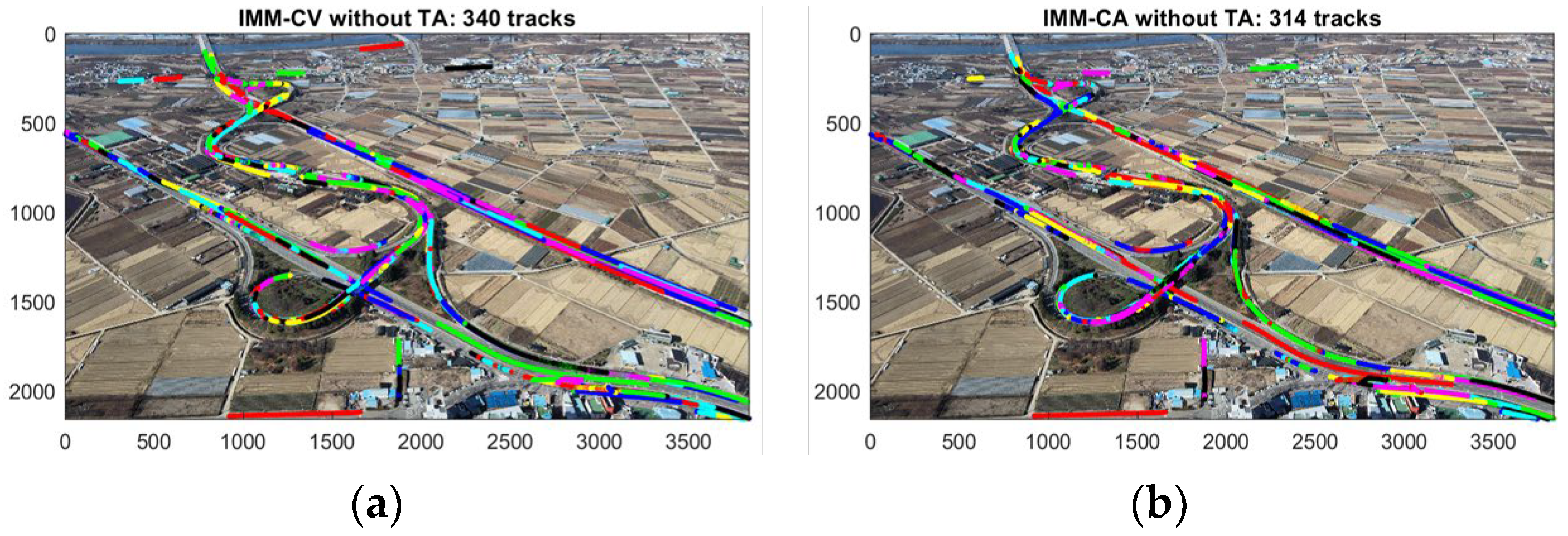
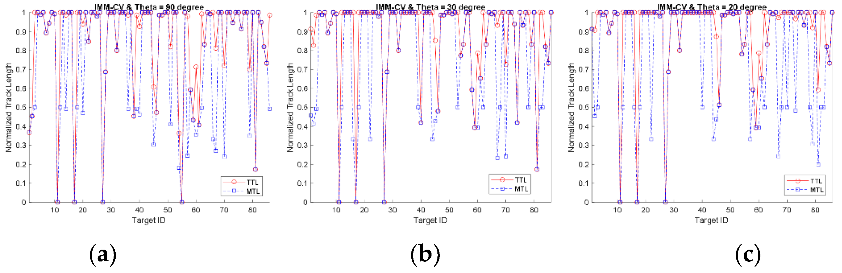
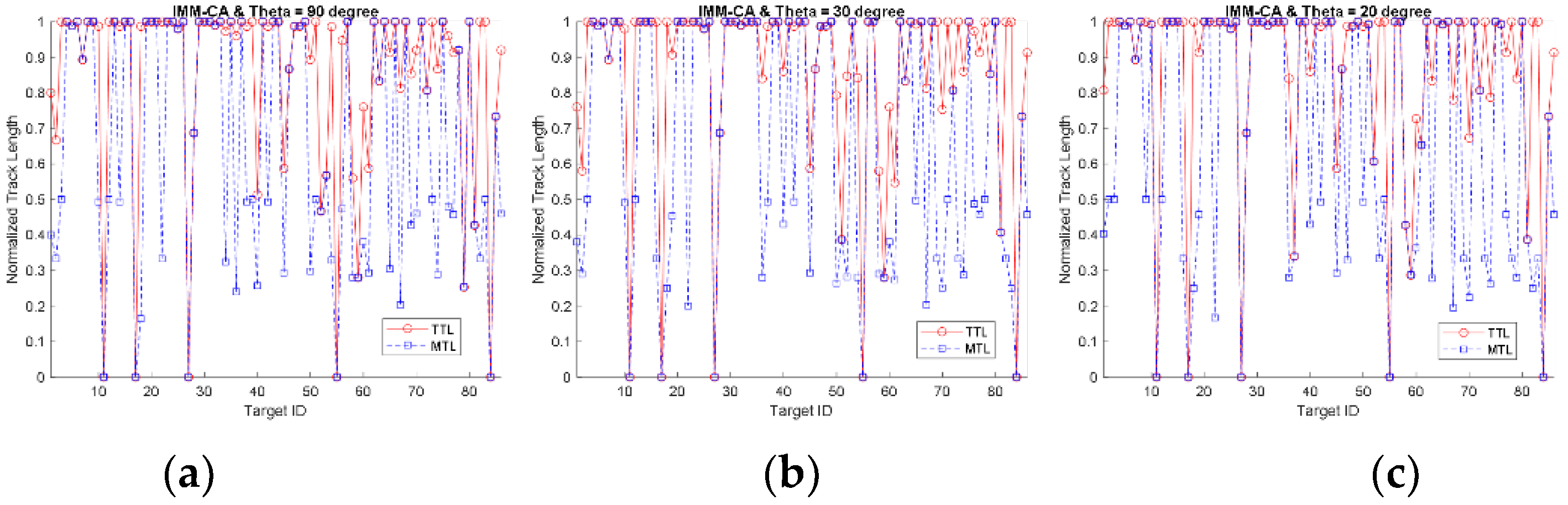
5.2. Multiple Target Tracking

The positions of Figure 9a become inputs to the target-tracking stage. The sampling time is 1/15 s since every second frame is processed. The IMM-CV and IMM-CA are adopted with the image-to-position conversion and the proposed directional track association procedure. Table 1 shows the parameters for target tracking; it is noted that the angular threshold θ g of 90° is equivalent to the track association without the directional gating.
For IMM-CV and IMM-CA without track association, a total of 340 and 314 valid tracks are generated, as shown in Figure 10a,b. The number of tracks of IMM-CV is reduced to 173, 185, and 192 by the directional track association when θ g is 90°, 30°, and 20°, respectively, as shown in Figure 11a–c. For IMM-CA, 196, 208, and 209 tracks are generated for the directional track associations when θ g is 90°, 30°, and 20°, respectively, as shown in Figure 12a–c.
Two metrics, TTL and MTL are employed to evaluate the tracking performance. The TTL and MTL are defined, respectively, as [30]:
TTL = Sum   of   lengths   of   tracks   which   have   the   same   target   ID Target   life   length 1 ,
MTL = TTL Number   of   tracks   associated   in   TTL .
A track’s target ID is defined as the target with the most measurements on the track. The MTL becomes less than the TTL in case of track breakage or overlap. The TTL and MTL are the same if only one track is generated for one target. The TTL and MTL are 0 if no track is generated for a target when the target is missing. Figure 13 and Figure 14 show the TTL and MTL of Figure 11 and Figure 12, respectively. Three targets (11, 17, 27) are missing in all cases. In addition, no tracks are set on Target 55 in Figure 13a and on Targets 55 and 84 in Figure 14a–c.
Table 2 and Table 3 show the overall tracking performance of IMM-CV and IMM-CA, respectively. They show the number of tracks, the number of tracks associated with the targets of interest, average TTL and MTL, average TTL and MTL excluding missing targets, and number of missing targets. The average TTL and MTL are, respectively, 84.9–91.0% and 65.6–78.2%. Excluding missing targets, the average TTL and MTL accounted for 89.2–94.3% and 69.7–81.0, respectively.
Eight supplementary multimedia files (MP4 format) for Figure 10, Figure 11 and Figure 12 is available online. The first is the IMM-CV without the track association for Figure 10a (Supplementary Material Video S1), and the second is the IMM-CA without the track association for Figure 10b (Supplementary Material Video S2). The third is the IMM-CV with θ g = 90 ° for Figure 11a (Supplementary Material Video S3). The fourth is the IMM-CV with θ g = 30 ° for Figure 11b (Supplementary Material Video S4). The fifth is the IMM-CV with θ g = 20 ° for Figure 11c (Supplementary Material Video S5). The sixth is the IMM-CA with θ g = 90 ° for Figure 12a (Supplementary Material Video S6). The seventh is the IMM-CA with θ g = 30 ° for Figure 12b (Supplementary Material Video S7). The eighth is the IMM-CA with θ g = 20 ° for Figure 12c (Supplementary Material Video S8). The black squares and numbers in the MP4 files are position estimates and track numbers, respectively, in the order they were initialized. For better visualization, odd numbers are shown in white, and even numbers in yellow. The blue dots are the detection positions including false alarms.

6. Discussion

The image-to-position conversion is an approximation showing a significant improvement in object detection. The reverse process is also possible, and the track is displayed in the frame after the reverse process.
The stability of the drone (camera) is important especially for oblique images where the position of the target can be concentrated or easily occluded; it can prevent false detections that result in false tracks and false track associations.
The proposed track selection can reduce the number of tracks from 340 to 173–192 for IMM-CV and from 314 to 196–209 for IMM-CA. Smaller angular threshold yields higher TTL and MTL, producing more tracks. The highest TTL and MTL excluding missing targets are, respectively, 94.3% and 81.0% for IMM-CA with θ g = 20 ° . Some targets are still detected and tracked outside the range of interest as shown in the videos.
The average number of missing targets is 3.33 and 5 for IMM-CV and IMM-CA, respectively. Targets 11 and 27 move too slowly. Target 17 is occluded by trees and shadows. In the experiments, the surveillance area was around 0.53 km2. It was more than twice as large as the area when the camera was pointed directly at the ground.

7. Conclusions

In this paper, two strategies were developed for multitarget tracking by a small drone. One is the image-to-position conversion based on the AFOV, tilt angle, and altitude of the camera. The other is the improved track association for densely distributed track environments. Both the IMM-CV and IMM-CA schemes achieve robust results in TTL and MTL.
The overall process is computationally efficient as it does not require high-resolution video streaming or storage and training on large-scale data. This system is suitable for security and surveillance for civil and military applications such as threat detection, vehicle counting and chasing, and traffic control. This method can be also applied to tracking other objects such as people or animals over long distances. Target tracking using moving drones from various perspectives remains a subject of future study.

Supplementary Materials

The following are available online at https://zenodo.org/record/5932718, Video S1: IMM-CV, Video S2: IMM-CA, Video S3: IMM-CV-90, Video S4: IMM-CV-30, Video S5: IMM-CV-20, Video S6: IMM-CA-90, Video S7: IMM-CA-30, Video S8: IMM-CA-20.

Funding

This research was supported by Daegu University Research Grant 2019.

Institutional Review Board Statement

Not applicable.

Informed Consent Statement

Not applicable.

Data Availability Statement

Not applicable.

Acknowledgments

Not applicable.

Conflicts of Interest

The author declared no conflict of interest.

References

  1. Alzahrani, B.; Oubbati, O.S.; Barnawi, A.; Atiquzzaman, M.; Alghazzawi, D. UAV assistance paradigm: State-of-the-art in applications and challenges. J. Netw. Comput. Appl. 2020, 166, 102706. [Google Scholar] [CrossRef]
  2. Zaheer, Z.; Usmani, A.; Khan, E.; Qadeer, M.A. Aerial surveillance system using UAV. In Proceedings of the 2016 Thirteenth International Conference on Wireless and Optical Communications Networks (WOCN), Hyderabad, India, 21–23 July 2016; pp. 1–7. [Google Scholar]
  3. Theys, B.; Schutter, J.D. Forward flight tests of a quadcopter unmanned aerial vehicle with various spherical body diameters. Int. J. Micro Air Veh. 2020, 12, 1–8. [Google Scholar] [CrossRef]
  4. Li, S.; Yeung, D.-Y. Visual object tracking for unmanned aerial vehicles: A benchmark and new motion models. In Proceedings of the Thirty-Frist AAAI Conference on Artificial Intelligence (AAAI-17), San Francisco, CA, USA, 4–9 February 2017; pp. 4140–4146. [Google Scholar]
  5. Du, D.; Qi, Y.; Yu, H.; Yang, Y.; Duan, K.; Li, G.; Zhang, W.; Huang, Q.; Tian, Q. The Unmanned Aerial Vehicle Benchmark: Object Detection and Tracking. Lect. Notes Comput. Sci. 2018, 375–391. [Google Scholar] [CrossRef] [Green Version]
  6. Zhang, H.; Lei, Z.; Wang, G.; Hwang, J. Eye in the Sky: Drone-Based Object Tracking and 3D Localization. In Proceedings of the 27th ACM International Conference on Multimedia, Nice, France, 21–25 October 2019; pp. 899–907. [Google Scholar] [CrossRef] [Green Version]
  7. Lo, L.-Y.; Yiu, C.H.; Tang, Y.; Yang, A.-S.; Li, B.; Wen, C.-Y. Dynamic Object Tracking on Autonomous UAV System for Surveillance Applications. Sensors 2021, 21, 7888. [Google Scholar] [CrossRef]
  8. Zhang, S.; Zhuo, L.; Zhang, H.; Li, J. Object Tracking in Unmanned Aerial Vehicle Videos via Multifeature Discrimination and Instance-Aware Attention Network. Remote. Sens. 2020, 12, 2646. [Google Scholar] [CrossRef]
  9. Kouris, A.; Kyrkou, C.; Bouganis, C.-S. Informed Region Selection for Efficient UAV-Based Object Detectors: Altitude-Aware Vehicle Detection with Cycar Dataset. In Proceedings of the IEEE/RSJ International Conference on Intelligent Robots and Systems (IROS), Macau, China, 4–9 November 2019; pp. 51–58. [Google Scholar]
  10. Kamate, S.; Yilmazer, N. Application of Object Detection and Tracking Techniques for Unmanned Aerial Vehicles. Proc. Comput. Sci. 2015, 61, 436–441. [Google Scholar] [CrossRef] [Green Version]
  11. Fang, P.; Lu, J.; Tian, Y.; Miao, Z. An Improved Object Tracking Method in UAV Videos. Procedia Eng. 2011, 15, 634–638. [Google Scholar] [CrossRef]
  12. Jianfang, L.; Hao, Z.; Jingli, G. A novel fast target tracking method for UAV aerial image. Open Phys. 2017, 15, 420–426. [Google Scholar] [CrossRef] [Green Version]
  13. Yang, J.; Tang, W.; Ding, Z. Long-Term Target Tracking of UAVs Based on Kernelized Correlation Filter. Mathematics 2021, 9, 3006. [Google Scholar] [CrossRef]
  14. Mueller, M.; Sharma, G.; Smith, N.; Ghanem, B. Persistent Aerial Tracking system for UAVs. In Proceedings of the 2016 IEEE/RSJ International Conference on Intelligent Robots and Systems (IROS), Daejeon, Korea, 9–14 October 2016; pp. 1562–1569. [Google Scholar] [CrossRef]
  15. Li, Y.; Doucette, E.A.; Curtis, J.W.; Gans, N. Ground target tracking and trajectory prediction by UAV using a single camera and 3D road geometry recovery. In Proceedings of the 2017 American Control Conference (ACC), Seattle, WA, USA, 24–26 May 2017; pp. 1238–1243. [Google Scholar] [CrossRef]
  16. Guido, G.; Gallelli, V.; Rogano, D.; Vitale, A. Evaluating the accuracy of vehicle tracking data obtained from Unmanned Aerial Vehicles. Int. J. Transp. Sci. Technol. 2016, 5, 136–151. [Google Scholar] [CrossRef]
  17. Rajasekaran, R.K.; Ahmed, N.; Frew, E. Bayesian Fusion of Unlabeled Vision and RF Data for Aerial Tracking of Ground Targets. In Proceedings of the IEEE/RSJ International Conference on Intelligent Robots and Systems (IROS), Las Vegas, NV, USA, 25–29 October 2020; pp. 1629–1636. [Google Scholar]
  18. Upadhyay, J.; Rawat, A.; Deb, D. Multiple Drone Navigation and Formation Using Selective Target Tracking-Based Computer Vision. Electronics 2021, 10, 2125. [Google Scholar] [CrossRef]
  19. Leira, F.S.; Helgensen, H.H.; Johansen, T.A.; Fossen, T.I. Object detection, recognition, and tracking from UAVs using a thermal camera. J. Field Robot. 2021, 38, 242–267. [Google Scholar] [CrossRef]
  20. Helgesen, H.H.; Leira, F.S.; Johansen, T.A. Colored-Noise Tracking of Floating Objects using UAVs with Thermal Cameras. In Proceedings of the 2019 International Conference on Unmanned Aircraft Systems (ICUAS), Atlanta, GA, USA, 11–14 June 2019; pp. 651–660. [Google Scholar] [CrossRef] [Green Version]
  21. Yeom, S.; Cho, I.-J. Detection and Tracking of Moving Pedestrians with a Small Unmanned Aerial Vehicle. Appl. Sci. 2019, 9, 3359. [Google Scholar] [CrossRef] [Green Version]
  22. Yeom, S.; Nam, D.-H. Moving Vehicle Tracking with a Moving Drone Based on Track Association. Appl. Sci. 2021, 11, 4046. [Google Scholar] [CrossRef]
  23. Yeom, S. Moving People Tracking and False Track Removing with Infrared Thermal Imaging by a Multirotor. Drones 2021, 5, 65. [Google Scholar] [CrossRef]
  24. Yeom, S. Long Distance Moving Vehicle Tracking with a Multirotor Based on IMM-Directional Track Association. Appl. Sci. 2021, 11, 11234. [Google Scholar] [CrossRef]
  25. Blom, H.A.P.; Bar-shalom, Y. The interacting multiple model algorithm for systems with Markovian switching coefficients. IEEE Trans. Autom. Control 1988, 33, 780–783. [Google Scholar] [CrossRef]
  26. Houles, A.; Bar-Shalom, Y. Multisensor Tracking of a Maneuvering Target in Clutter. IEEE Trans. Aerospace Electron. Syst. 1989, 25, 176–189. [Google Scholar] [CrossRef]
  27. Bar-Shalom, Y.; Li, X.R. Multitarget-Multisensor Tracking: Principles and Techniques; YBS Publishing: Storrs, CT, USA, 1995. [Google Scholar]
  28. Babinec, A.; Jiří, A. On accuracy of position estimation from aerial imagery captured by low-flying UAVs. Int. J. Transp. Sci. Technol. 2016, 5, 152–166. [Google Scholar] [CrossRef]
  29. Cai, Y.; Ding, Y.; Zhang, H.; Xiu, J.; Liu, Z. Geo-Location Algorithm for Building Targets in Oblique Remote Sensing Images Based on Deep Learning and Height Estimation. Remote Sens. 2020, 12, 2427. [Google Scholar] [CrossRef]
  30. Yeom, S.-W.; Kirubarajan, T.; Bar-Shalom, Y. Track segment association, fine-step IMM and initialization with doppler for improved track performance. IEEE Trans. Aerosp. Electron. Syst. 2004, 40, 293–309. [Google Scholar] [CrossRef]
  31. Li, X.R.; Jilkov, V.P. Survey of maneuvering target tracking, part I: Dynamic models. IEEE Trans. Aerosp. Electron. Syst. 2003, 39, 1333–1364. [Google Scholar]
  32. Available online: https://map.naver.com/v5/search/%EA%B2%BD%EC%82%B0ic?c=14336187.1023075,4283701.1549134,15,0,0,1,dh (accessed on 31 January 2022).
Figure 1. Block diagram of moving object detection and multiple target tracking.
Drones 06 00055 g001
Figure 2. Three sample scenes showing targets: (a) sample frame; (b) sample scene 1; (c) sample scene 2; (d) sample scene 3.
Drones 06 00055 g002
Figure 3. Coordinate conversion from image to real-world: (a) x direction; (b) y direction.
Drones 06 00055 g003
Figure 4. Approximated conversion from image to real world, (a) visualization of the coordinate conversion; (b) actual pixel size.
Drones 06 00055 g004
Figure 5. Block diagram of multiple target tracking.
Drones 06 00055 g005
Figure 6. Illustration of track association at a frame: fused tracks in blue and potentially terminated tracks in yellow.
Drones 06 00055 g006
Figure 7. (a) Targets 1–53 at the first frame; (b) Targets 54–86 at the first frame; (c) 1 km range of the drone with approximated view angles.
Drones 06 00055 g007aDrones 06 00055 g007b
Figure 8. Object detection: (a) frame subtraction and thresholding; (b) morphological operation (closing) of (a); (c) basic rectangles after false alarm removal of (b); (d) 127 centers of basic rectangles of (c), indicated as blue dots.
Drones 06 00055 g008
Figure 9. Object detection results of 151 frames with: (a) image-to-position conversion; (b) maximum pixel size; (c) median pixel size; (d) minimum pixel size.
Drones 06 00055 g009
Figure 10. All tracks without track association: (a) IMM-CV; (b) IMM-CA.
Drones 06 00055 g010
Figure 11. All tracks with track association, IMM-CV: (a) θ g = 90 ° ; (b) θ g = 30 ° ; (c) θ g = 20 ° .
Drones 06 00055 g011
Figure 12. All tracks with track association, IMM-CA: (a) θ g = 90 ° ; (b) θ g = 30 ° ; (c) θ g = 20 ° .
Drones 06 00055 g012
Figure 13. TTL and MLT of IMM-CV: (a) θ g = 90 ° ; (b) θ g = 30 ° ; (c) θ g = 20 ° .
Drones 06 00055 g013
Figure 14. TTL and MLT of IMM-CA: (a) θ g = 90 ° ; (b) θ g = 30 ° ; (c) θ g = 20 ° .
Drones 06 00055 g014
Table 1. Parameters for target tracking.
ParametersIMM-CVIMM-CA
Sampling time1/15 s
Max. target speed for initialization, Vmax60 m/s
Process noise variance σ 1 x = σ 1 y 1 m/s20.01 m/s2
σ 2 x = σ 2 y 10 m/s20.1 m/s2
Mode transition probabiltiy pij [ 0.8    0.2 0.3    0.7 ]
Measurement   noise   variance ,   r x = r y 1.5 m
Measurent association Gate   threshold ,   γ f 8
Max. target speed, Smax80 m/s
Track association Gate   threshold ,   γ g 100
Anguar   threhold ,   θ g 90°, 30°, 20°
Track terminationMax. searching number20 frames (1.33 s)
Min. target speed1 m/s
Min. track life length for track validity 20   frames   ( 1.33   s )
Table 2. Tracking performance of IMM-CV.
IMM-CV
θ g = 90 ° θ g = 30 ° θ g = 20 °
Number of tracks173185192
Number of associated tracks106108111
Avg. TTL0.8510.8850.910
Avg. MTL0.7470.7700.782
Avg. TTL w/o missing targets0.8920.91760.943
Avg. MTL w/o missing targets0.7830.7980.810
Number of missing targets433
Table 3. Tracking performance of IMM-CA.
IMM-CA
θ g = 90 ° θ g = 30 ° θ g = 20 °
Number of tracks196208209
Number of associated tracks129133133
Avg. TTL0.8490.8580.861
Avg. MTL0.6560.6600.668
Avg. TTL w/o missing targets0.9010.9110.914
Avg. MTL w/o missing targets0.6970.7000.709
Number of missing targets555
Publisher’s Note: MDPI stays neutral with regard to jurisdictional claims in published maps and institutional affiliations.

