Ergodic Performance Analysis of Double Intelligent Reflecting Surfaces-Aided NOMA–UAV Systems with Hardware Impairment

Abstract

In this work, we design an intelligent reflecting surface (IRS)-assisted Internet of Things (IoT) by enabling non-orthogonal multiple access (NOMA) and unmanned aerial vehicles (UAV) approaches. We pay attention to studying the achievable rates for the ground users. A practical system model takes into account the presence of hardware impairment when Rayleigh and Rician channels are adopted for the IRS–NOMA–UAV system. Our main findings are presented to showcase the exact expressions for achievable rates, and then we derive their simple approximations for a more insightful performance evaluation. The validity of these approximations is demonstrated using extensive Monte Carlo simulations. We confirm the achievable rate improvement decided by main parameters such as the average signal to noise ratio at source, the position of IRS with respect to the source and destination and the number of IRS elements. As a suggestion for the deployment of a low-cost IoT system, the double-IRS model is a reliable approach to realizing the system as long as the hardware impairment level is controlled. The results show that the proposed scheme can greatly improve achievable rates, obtain optimal performance at one of two devices and exhibit a small performance gap compared with the other benchmark scheme.

1. Introduction

In recent years, as a promising transmission method, the new generation wireless systems can rely on IRS and UAV to enhance their spectral and energy efficiency since IRS is examined as a cost-effective deployment approach [1,2,3]. Specifically, by varying the amplitude and phase for the incident signal, an IRS leverages its low-cost reconfigurable passive elements to reflect signals to distant users effectively [4,5]. The system relying on IRS can enhance the link quality and enlarge the coverage significantly when IRS is able to adjust amplitude-reflection coefficients and phase-shift variables appropriately [6,7,8]. The authors in [7] studied secure IRS–UAV systems by integrating IRS with UAV in wireless networks, which are susceptible to eavesdropping related to air-ground line-of-sight channels. To facilitate security, IRS can be leveraged due to its capability of reconfiguring the propagation environment, and thus IRS helps to reduce the impacts of eavesdroppers. The secure transmission of an IRS-assisted UAV network is analyzed under the impact of an eavesdropper. The transmit beamforming, the trajectory of UAV and the phase shift of IRS can be optimized to further obtain maximal rates [7]. Besides, IRS has two prominent features—passive reflection with low power consumption and the operation of full-duplex (FD) mode without self-interference—and these benefits are crucial in comparison with conventional approaches—for example, relaying networks [9].

To further increase energy and spectrum efficiency, the power-domain NOMA technology has been studied as a potential technique for IoT applications [10,11]. The NOMA architecture can be described as follows. In the transmit side of a NOMA system, different amounts of power at the transmitter or the base station (BS) are assigned to multiple users when superimposing signal processing, while those users share the same orthogonal resources such as frequency, time and spreading code. At the receiver side associated with a downlink, demultiplexing the transmitted signals is conducted by employing successive interference cancellation (SIC) [12]. To decode the needed signals, the user treats all the weaker user signals as interference; then, its own signal can be decoded in the last step [13,14,15]. In contrast to the downlink, the common receiver or the BS achieves a signal in an uplink, allowing multiple users to consume the common communication. This means that all users send a superposed signal comprising the signals of these users toward the BS. For signal detection, the BS needs the assistance of SIC to decode the signals of the transmitting users [12]. In this way, a higher number of users can be served in the context of NOMA, which exhibits a significant improvement compared with the conventional orthogonal multiple access (OMA)-aided transmission approach [11].

The combination of IRS and NOMA could be a prominent technique to leverage energy-efficient and low-cost deployment [16,17,18,19,20,21,22,23,24,25]. The authors in [16] designed an IRS–NOMA system by considering both continuous phase shifting and discrete phase shifting corresponding to the ideal IRS and the non-ideal IRS circumstance. To demonstrate performance, closed-form expressions are derived to examine the average required transmit power, the outage probability and the diversity order by benefiting from the Laguerre series and the isotropic random vector. In demonstrated analytical results, the BS antenna number and the IRS element number are consistently affected by varying the transmit power. In [17], IRS-aided simultaneous wireless information and power transfer (SWIPT) NOMA networks are studied. In particular, a problem of minimizing the transmit power at the BS can be solved by jointly optimizing the BS transmit beamforming vector, power splitting (PS) ratio, SIC decoding order and IRS phase shift. This optimization is guaranteed to satisfy the energy harvested threshold of each user and the quality-of-service (QoS) constraint. To improve the performance of multiple user equipments (UEs), the BS utilizes the UAV-mounted IRS to flexibly serve ground users [18]. The direct non-line-of-sight links between the BS and UEs are required to power the IRS relaying links. The main performance metric is presented, i.e., the outage probability. The model of IRS–NOMA in [19] allows this cell-edge user to be paired with a cell-center user to form the NOMA scheme. In this way, the coverage can be improved at the cell-edge user. The phase shift plays an important role in the design of an IRS-aided NOMA system, i.e., the impacts of random phase shifting and coherent phase shifting are further investigated [20]. In [21], IRS-assisted NOMA benefits from enabling BS’s beamforming vectors. To minimize transmission power, the beamforming vectors and the IRS phase shift matrix could be optimized. One can place the IRS at preferred locations, and line-of-sight (LoS) can be adopted for the links between the transmitters and the IRS before reflecting to receivers [23,24,25]. The links can be enhanced if the system enables LoS and optimized passive beamforming vectors to implement a NOMA-assisted IRS. In [23], by considering ideal and non-ideal IRSs, the system performance was evaluated for the link from source to destination via IRS. In [24], a tremendous performance improvement could be confirmed in the approach of an IRS-assisted NOMA system. This means that IRS-assisted NOMA exhibits sufficient benefits to be incorporated into the existing IoT systems.

1.1. Related Works

In similar work, the authors of [26] presented a hybrid aerial FD relaying protocol consisting of a IRS mounted UAV system. To help the information transfer between the base station and multiple users, the UAV acts as a relay operating in the decode and forward mode. The study also presented the closed-form formulas of achievable throughput, outage probability and ergodic capacity. The authors in [27] studied IRS-assisted multi-user multiple-input single-output (MISO) wireless systems by considering the ergodic capacity in both uplink and downlink scenarios. They examined the realistic case of statistical instantaneous channel state information (CSI). Further, analytical expressions of the ergodic sum capacity were derived as the main contribution. In [28], a two-IRS system was studied by employing the centralized and the distributed modes corresponding to the reflecting elements being mounted at a single IRS, and multiple IRSs were designed with the same number of reflecting elements. To examine the benefits of the two-IRS model, the closed-form approximation expressions of the ergodic capacity were derived along with their tight upper and lower bounds to provide more necessary insights. Although the transmit power and the Rician-K factor have the main influences on the system performance, selected modes of the centralized IRS result in a better ergodic capacity as compared with the distributed IRS mode. It is worth noting that the location of the IRS has strong impacts on ergodic performance. Therefore, a multiple IRS design for IoT is necessary.

1.2. Motivations and Our Contributions

In contrast to [27,28], Nakagami-m fading channels are deployed for an IRS-aided system in a recent work [29]. The performance is decided by two phase configuration designs including random and coherent phase shifting. As the main performance metrics, the authors in [29] derived formulas of the outage behavior and the bit error rate when binary modulation schemes are applied. The closed-form approximations for the ergodic capacity are extra performance evaluations. However, we first need to answer how many IRSs are sufficient to obtain the expected achievable rate. Secondly, Rayeligh and Rician channels could be applied for several practical situations of UAV. Therefore, this study prefers to examine the achievable rate in practical scenarios where hardware impairment is a key factor in degraded performance. We can summarize our contributions as follows.

• We consider an IRS–NOMA–UAV system without direct links, which consists of a source and several IRSs. We focus on the performance analysis of a group of two users and further determine the impact of hardware impairment.
• We derive closed-form expressions for the achievable rates for two NOMA users under the channel models of Rayleigh and Rician. Compared with recent work [30], our result could be combined with their result to provide complete ergodic performance analysis in a more practical circumstance.
• We employ Monte Carlo simulations to validate the analytical outage probabilities. The achievable rate of each user mainly depends on power allocation factors rather than other main parameters such as the number of IRSs, the number of meta-surface elements and the IRS reflecting coefficient.

The remainder of this article is organized as follows. In Section 2, a double IRS–NOMA–UAV system model is described, and the respective received signal with hardware impairment is formulated. We provide the derivation of closed-form ergodic achievable rates for a group of IoT users in Section 3. We aim to verify the results of computations in Section 4. Finally, we summarize concluding remarks and future research in Section 5.

2. System Model

We aim to design a IoT network by enabling IRS, NOMA and UAV techniques, where a single antenna source $\left(S\right)$ powers the signal transmission by IRS to serve many users at destinations. The IRSs are mounted in UAVs for better transmission from the base station to ground users. These ground users are divided into many groups, and a considered group contains two users $(D_i;i=1,2)$. The system can maximize the benefits of IRS if multiple I IRSs are deployed, as shown in Figure 1. It is assumed that there is no direct path between the source S and ground users (destinations). To reduce the cost of the design, we refer to the first scenario where two IRSs, i.e., $I_1$ and $I_2$, possess reflecting elements $N_1$ and $N_2$. Those IRSs are placed at specific locations (i.e., buildings) to reflect passive beamforming signals towards the destinations (IoT devices). We need to answer how many IRSs are required to achieve the best performance at destinations. Therefore, we move our attention to the second scenario (the benchmark) by assigning three IRSs, i.e., $I_1$, $I_2$ and $I_3$, which are installed with reflecting elements $N_1$, $N_2$ and $N_3$, respectively (it is reasonable to design double-IRS due to cost efficiency in deployment. Although multi-IRS was developed in [31], the numerical result demonstrated a small gap between the double-IRS and three-IRSs case. Therefore, in this study, we emphasize the performance for two scenarios of IRSs).

We denote the (scalar) channels from the S to the IRSs, and from the IRSs to $D_i$, respectively, as $h_{S{I}_u,n}^{}$ and $h_{I_u{D}_i,n}$. The hardware impairment at the S is denoted as ${\tau }_S\sim CN\left(0,{\mathrm{{\rm Y}}}_S^{2}P\right)$, where ${\mathrm{{\rm Y}}}_S$ represents the proportionality coefficients, which describe the severity of the distortion noises at S. The hardware impairments at the $D_i$ is ${\tau }_{D_{ui}}\sim CN\left(0,{\mathrm{{\rm Y}}}_{D_i}^{2}P{\left|{\displaystyle \sum _{u=1}^I}{\displaystyle \sum _{n=1}^{N_u}}{h}_{S{I}_u,n}^{}{h}_{I_u{D}_i,n}{\eta }_{un}{e}^{j{\theta }_{un}^{\left(D_i\right)}}\right|}^2\right)$ [32], where ${\mathrm{{\rm Y}}}_{D_i}$ represents the proportionality coefficients. Here, ${\mathrm{{\rm Y}}}_{D_i}$ is associated with the distortion noises at $D_i$. Then, the overall received signal at the user $D_i$ with multiple I IRSs is given as [30,33]

$$\begin{array}{c}{y}_{D_i}={\displaystyle \sum _{u=1}^I}{\displaystyle \sum _{n=1}^{N_u}}{h}_{S{I}_u,n}^{}{h}_{I_u{D}_i,n}{\eta }_{un}{e}^{j{\theta }_{un}^{\left(D_i\right)}}\left(\sqrt{P{\chi }_1}{x}_1+\sqrt{P{\chi }_2}{x}_2+{\tau }_S\right)+{\tau }_{D_{ui}}+n_{D_i},\hfill \end{array}$$

(1)

where P is the total transmit power at the source, $x_i$ is the transmitted signal by source, ${\chi }_i$ denotes the power allocation factor for message $x_i$ with ${\chi }_1+{\chi }_2=1$, ${\chi }_1>{\chi }_2$ [34], ${\theta }_{un}^{\left(D_i\right)}$ is the adjustable phase applied by the n-th reflecting element of the $S-I-D_i$, ${\eta }_{un}$ is the reflection coefficients of I with ${\eta }_{un}\in \left(0,1\right]$, and $n_{D_i}$ stands for the circularly symmetric additive White Gaussian noise (AWGN) with zero mean and variance ${\sigma }_n^2$, i.e., $n_{D_i}\sim \mathcal{CN}\left(0,{\sigma }_n^2\right)$.

2.1. The First Scenario

The system has two hops from source to IRS and from IRS to destinations. These links are demonstrated in the system model, i.e., $h_{S{I}_1,n}^{}$, $h_{I_1{D}_1,n}$, $h_{S{I}_2,n}^{}$ and $h_{I_2{D}_1,n}$, along with their channel gains, denoted as $h_{S{I}_1,n}=d_{S{I}_1}^{-\alpha /2}{\overline{h}}_{S{I}_1,n}{e}^{-j{\varphi }_{1n}}$, $h_{I_1{D}_1,n}=d_{I_1{D}_1}^{-\alpha /2}{\overline{h}}_{I_1{D}_1,n}{e}^{-j{\delta }_{1n}^{\left(D_1\right)}}$, $h_{S{I}_2,n}=d_{S{I}_2}^{-\alpha /2}{\overline{h}}_{S{I}_2,n}{e}^{-j{\varphi }_{2n}}$ and $h_{I_2{D}_1,n}=d_{I_2{D}_1}^{-\alpha /2}{\overline{h}}_{I_2{D}_1,n}{e}^{-j{\delta }_{2n}^{\left(D_1\right)}}$ [35]; the links $S-I_1$, $I_1-D_1$, $S-I_2$ and $I_2-D_1$ are associated with distances $d_{S{I}_1}^{}$, $d_{I_1{D}_1}^{}$, $d_{S{I}_2}^{}$ and $d_{I_2{D}_1}^{}$, respectively. Here, the path-loss coefficient is $\alpha$, while ${\varphi }_{1n}$ and ${\varphi }_{2n}$ and ${\delta }_{1n}^{\left(D_1\right)}$ and ${\delta }_{2n}^{\left(D_1\right)}$ are the phases of the channel gains. ${\overline{h}}_{S{I}_1,n}$, ${\overline{h}}_{I_1{D}_1,n}$, ${\overline{h}}_{S{I}_2,n}$ and ${\overline{h}}_{I_2{D}_1,n}$ are the amplitudes of the channel gains, and they are adopted with a Rayleigh distribution. In the scope of our paper, it is reasonable to assume that the IRS achieves the full knowledge of the channels $h_{S{I}_1,n}^{}$, $h_{I_1{D}_1,n}$, $h_{S{I}_2,n}^{}$ and $h_{I_2{D}_1,n}$.

The overall received signal at user $D_1$ is given as [36]

$$\begin{array}{c}{y}_{D_1}^{\left(1\right)}=\left({\displaystyle \sum _{n=1}^{N_1}}{h}_{S{I}_1,n}^{}{h}_{I_1{D}_1,n}{\eta }_{1n}{e}^{j{\theta }_{1n}^{\left(D_1\right)}}\right.\left.+{\displaystyle \sum _{n=1}^{N_2}}{h}_{S{I}_2,n}^{}{h}_{I_2{D}_1,n}{\eta }_{2n}{e}^{j{\theta }_{2n}^{\left(D_1\right)}}\right)\left(\sqrt{P{\chi }_1}{x}_1+\sqrt{P{\chi }_2}{x}_2+{\tau }_S\right)+{\tau }_{D_{21}}+n_{D_1},\hfill \end{array}$$

(2)

where ${\theta }_{1n}^{\left(D_1\right)}$ is the adjustable phase applied by the nth reflecting element of $S-I_1-D_1$, ${\theta }_{2n}^{\left(D_1\right)}$ stands for the adjustable phase applied by the nth reflecting element of $S-I_2-D_1$, ${\eta }_{1n}$ is the reflection coefficient of $I_1$ with ${\eta }_{1n}\in \left(0,1\right]$, and ${\eta }_{2n}$ represents the reflection coefficients of $I_2$ with ${\eta }_{2n}\in \left(0,1\right]$.

The hardware impairment at the $D_1$ is denoted as [32]

$$\begin{array}{c}{\tau }_{D_{21}}\sim CN\left(0,{\mathrm{{\rm Y}}}_{D_1}^{2}P\left|{\displaystyle \sum _{n=1}^{N_1}}{h}_{S{I}_1,n}^{}{h}_{I_1{D}_1,n}{\eta }_{1n}{e}^{j{\theta }_{1n}^{\left(D_1\right)}}\right.\right.\left.{\left.+{\displaystyle \sum _{n=1}^{N_2}}{h}_{S{I}_2,n}^{}{h}_{I_2{D}_1,n}{\eta }_{2n}{e}^{j{\theta }_{2n}^{\left(D_1\right)}}\right|}^2\right).\hfill \end{array}$$

(3)

The received signal to noise plus distortion ratio (SNDR) at the destination $D_1$ is defined as

$$\begin{array}{c}{\gamma }_{D_1}^{\left(1\right)}=\frac{\gamma {\chi }_1{\left|A_1^{\left(1\right)}{e}^{j\left({\theta }_{1n}^{\left(D_1\right)}-{\varphi }_{1n}-{\delta }_{1n}^{\left(D_1\right)}\right)}+A_2^{\left(1\right)}{e}^{j\left({\theta }_{2n}^{\left(D_1\right)}-{\varphi }_{2n}-{\delta }_{2n}^{\left(D_1\right)}\right)}\right|}^2}{\gamma {\chi }_2{\left|A_1^{\left(1\right)}{e}^{j\left({\theta }_{1n}^{\left(D_1\right)}-{\varphi }_{1n}-{\delta }_{1n}^{\left(D_1\right)}\right)}+A_2^{\left(1\right)}{e}^{j\left({\theta }_{2n}^{\left(D_1\right)}-{\varphi }_{2n}-{\delta }_{2n}^{\left(D_1\right)}\right)}\right|}^2+\left({\mathrm{{\rm Y}}}_S^2+{\mathrm{{\rm Y}}}_{D_1}^2\right)\gamma {\left|A_1^{\left(1\right)}{e}^{j\left({\theta }_{1n}^{\left(D_1\right)}-{\varphi }_{1n}-{\delta }_{1n}^{\left(D_1\right)}\right)}+A_2^{\left(1\right)}{e}^{j\left({\theta }_{2n}^{\left(D_1\right)}-{\varphi }_{2n}-{\delta }_{2n}^{\left(D_1\right)}\right)}\right|}^2+1},\hfill \end{array}$$

(4)

where $\gamma =\frac{P}{{\sigma }_n^2}$ is the average signal-to-noise ratio (SNR) at the source, $A_1^{\left(1\right)}=d_{S{I}_1}^{-\alpha /2}{d}_{I_1{D}_1}^{-\alpha /2}{\displaystyle \sum _{n=1}^{N_1}}{\overline{h}}_{S{I}_1,n}{\overline{h}}_{I_1{D}_1,n}{\eta }_{1n}$, $A_2^{\left(1\right)}=d_{S{I}_2}^{-\alpha /2}{d}_{I_2{D}_1}^{-\alpha /2}{\displaystyle \sum _{n=1}^{N_2}}{\overline{h}}_{S{I}_2,n}{\overline{h}}_{I_2{D}_1,n}{\eta }_{2n}$, ${\eta }_{1n}=\eta ,{\forall }_{1n}$ and ${\eta }_{2n}=\eta ,{\forall }_{2n}$.

It is noted that from (4) that the highest value of ${\gamma }_{D_1}^{\left(1\right)}$ can be obtained by disregarding the channel phases. In this case, the phases can be modified as ${\theta }_{1n}^{\left(D_1\right)}={\varphi }_{1n}+{\delta }_{1n}^{\left(D_1\right)}$ for $1n=1,\dots ,N_1$ and ${\theta }_{2n}^{\left(D_1\right)}={\varphi }_{2n}+{\delta }_{2n}^{\left(D_1\right)}$ for $2n=1,\dots ,N_2$ [35], while the maximal ${\gamma }_{D_1}^{\left(1\right)}$ can be written as

$${\gamma }_{D_1}^{\left(1\right)}=\frac{\gamma {\chi }_1{\left|A_1^{\left(1\right)}+A_2^{\left(1\right)}\right|}^2}{\gamma {\chi }_2{\left|A_1^{\left(1\right)}+A_2^{\left(1\right)}\right|}^2+\left({\mathrm{{\rm Y}}}_S^2+{\mathrm{{\rm Y}}}_{D_1}^2\right)\gamma {\left|A_1^{\left(1\right)}+A_2^{\left(1\right)}\right|}^2+1}.$$

(5)

The achievable rate for the $D_1$ is given as

$$R_{D_1}^{\left(1\right)}={log}_2\left(1+{\gamma }_{D_1}^{\left(1\right)}\right).$$

(6)

The overall received signal at the user $D_2$ is given as [36]

$$\begin{array}{c}{y}_{D_2}^{\left(1\right)}=\left({\displaystyle \sum _{n=1}^{N_1}}{h}_{S{I}_1,n}^{}{h}_{I_1{D}_2,n}{\eta }_{1n}{e}^{j{\theta }_{1n}^{\left(D_2\right)}}\right.\left.+{\displaystyle \sum _{n=1}^{N_2}}{h}_{S{I}_2,n}^{}{h}_{I_2{D}_2,n}{\eta }_{2n}{e}^{j{\theta }_{2n}^{\left(D_2\right)}}\right)\left(\sqrt{P{\chi }_1}{x}_1+\sqrt{P{\chi }_2}{x}_2+{\tau }_S\right)+{\tau }_{D_{22}}+n_{D_2},\hfill \end{array}$$

(7)

where ${\theta }_{1n}^{\left(D_2\right)}$ stands for the adjustable phase applied by the nth reflecting element of the $S-I_1-D_2$, and ${\theta }_{2n}^{\left(D_2\right)}$ is the adjustable phase applied by the nth reflecting element of the $S-I_2-D_2$. In addition, $h_{I_1{D}_2,n}$ and $h_{I_2{D}_2,n}$ are the channel gains with $h_{I_1{D}_2,n}=d_{I_1{D}_2}^{-\alpha /2}{\overline{h}}_{I_1{D}_2,n}{e}^{-j{\delta }_{1n}^{\left(D_2\right)}}$ and $h_{I_2{D}_2,n}=d_{I_2{D}_2}^{-\alpha /2}{\overline{h}}_{I_2{D}_2,n}{e}^{-j{\delta }_{2n}^{\left(D_2\right)}}$ [35], where $d_{I_1{D}_2}^{}$ and $d_{I_2{D}_2}^{}$ are the distances for the $I_1-D_2$ link and $I_2-D_2$ link, respectively, and ${\delta }_{1n}^{\left(D_2\right)}$ and ${\delta }_{2n}^{\left(D_2\right)}$ are the phases of the channel gains. ${\overline{h}}_{I_1{D}_2,n}$ and ${\overline{h}}_{I_2{D}_2,n}$ following a Rayleigh distribution are the amplitudes of the channel gains. Moreover, we assume that the IRS has the full knowledge of the channel phases of $h_{I_1{D}_2,n}$ and $h_{I_2{D}_2,n}$. The hardware impairments at the $D_2$ is denoted as [35]

$$\begin{array}{c}{\tau }_{D_{22}}\sim CN\left(0,{\mathrm{{\rm Y}}}_{D_2}^{2}P\left|{\displaystyle \sum _{n=1}^{N_1}}{h}_{S{I}_1,n}^{}{h}_{I_1{D}_2,n}{\eta }_{1n}{e}^{j{\theta }_{1n}^{\left(D_2\right)}}\right.\right.\left.{\left.+{\displaystyle \sum _n^{N_2}}{h}_{S{I}_2,n}^{}{h}_{I_2{D}_2,n}{\eta }_{2n}{e}^{j{\theta }_{2n}^{\left(D_2\right)}}\right|}^2\right).\hfill \end{array}$$

(8)

The resulting SNDR at the second user $D_2$ to decode $x_1$ can be formulated as

$$\begin{array}{c}{\gamma }_{x_1,D_2}^{\left(1\right)}=\frac{\gamma {\chi }_1{\left|B_1^{\left(1\right)}{e}^{j\left({\theta }_{1n}^{\left(D_2\right)}-{\varphi }_{1n}-{\delta }_{1n}^{\left(D_2\right)}\right)}+B_2^{\left(1\right)}{e}^{j\left({\theta }_{2n}^{\left(D_2\right)}-{\varphi }_{2n}-{\delta }_{2n}^{\left(D_2\right)}\right)}\right|}^2}{\gamma {\chi }_2{\left|B_1^{\left(1\right)}{e}^{j\left({\theta }_{1n}^{\left(D_2\right)}-{\varphi }_{1n}-{\delta }_{1n}^{\left(D_2\right)}\right)}+B_2^{\left(1\right)}{e}^{j\left({\theta }_{2n}^{\left(D_2\right)}-{\varphi }_{2n}-{\delta }_{2n}^{\left(D_2\right)}\right)}\right|}^2+\left({\mathrm{{\rm Y}}}_S^2+{\mathrm{{\rm Y}}}_{D_2}^2\right)\gamma {\left|B_1^{\left(1\right)}{e}^{j\left({\theta }_{1n}^{\left(D_2\right)}-{\varphi }_{1n}-{\delta }_{1n}^{\left(D_2\right)}\right)}+B_2^{\left(1\right)}{e}^{j\left({\theta }_{2n}^{\left(D_2\right)}-{\varphi }_{2n}-{\delta }_{2n}^{\left(D_2\right)}\right)}\right|}^2+1},\hfill \end{array}$$

(9)

where $B_1^{\left(1\right)}=d_{S{I}_1}^{-\alpha /2}{d}_{I_1{D}_2}^{-\alpha /2}\eta {\displaystyle \sum _{n=1}^{N_1}}{\overline{h}}_{S{I}_1,n}{\overline{h}}_{I_1{D}_2,n}$, $B_2^{\left(1\right)}=d_{S{I}_2}^{-\alpha /2}{d}_{I_2{D}_2}^{-\alpha /2}\eta {\displaystyle \sum _{n=1}^{N_2}}{\overline{h}}_{S{I}_2,n}{\overline{h}}_{I_2{D}_2,n}$.

In (9), to obtain the maximum value of ${\gamma }_{x_1,D_2}^{\left(1\right)}$, we need to eliminate the channel phases. Similar to the method in [35], by setting the phases ${\theta }_{1n}^{\left(D_2\right)}={\varphi }_{1n}+{\delta }_{1n}^{\left(D_2\right)}$ and ${\theta }_{2n}^{\left(D_2\right)}={\varphi }_{2n}+{\delta }_{2n}^{\left(D_2\right)}$, the maximal ${\gamma }_{x_1,D_2}^{\left(1\right)}$ can be written as

$$\begin{array}{c}{\gamma }_{x_1,D_2}^{\left(1\right)}=\frac{\gamma {\chi }_1{\left|B_1^{\left(1\right)}+B_2^{\left(1\right)}\right|}^2}{\gamma {\chi }_2{\left|B_1^{\left(1\right)}+B_2^{\left(1\right)}\right|}^2+\left({\mathrm{{\rm Y}}}_S^2+{\mathrm{{\rm Y}}}_{D_2}^2\right)\gamma {\left|B_1^{\left(1\right)}+B_2^{\left(1\right)}\right|}^2+1}.\hfill \end{array}$$

(10)

After SIC, the resulting SNDR at the user $D_2$ to decode $x_2$ can be formulated as

$${\gamma }_{x_2,D_2}^{\left(1\right)}=\frac{\gamma {\chi }_2{\left|B_1^{\left(1\right)}+B_2^{\left(1\right)}\right|}^2}{\left({\mathrm{{\rm Y}}}_S^2+{\mathrm{{\rm Y}}}_{D_2}^2\right)\gamma {\left|B_1^{\left(1\right)}+B_2^{\left(1\right)}\right|}^2+1}.$$

(11)

The achievable rate for the $D_2$ is given as

$$R_2^{\left(1\right)}={log}_2\left(1+min\left\{{\gamma }_{x_1,D_2}^{\left(1\right)},{\gamma }_{x_2,D_2}^{\left(1\right)}\right\}\right).$$

(12)

2.2. The Second Scenario (the Benchmark)

The overall received signal at the user $D_1$ is given as [33,36]

$$\begin{array}{c}{y}_{D_1}^{\left(2\right)}=\left({\displaystyle \sum _{n=1}^{N_1}}{h}_{S{I}_1,n}^{}{h}_{I_1{D}_1,n}{\eta }_{1n}{e}^{j{\theta }_{1n}^{\left(D_1\right)}}\right.+{\displaystyle \sum _{n=1}^{N_2}}{h}_{S{I}_2,n}^{}{h}_{I_2{D}_1,n}{\eta }_{2n}{e}^{j{\theta }_{2n}^{\left(D_1\right)}}\left.+{\displaystyle \sum _{n=1}^{N_3}}{h}_{S{I}_3,n}^{}{h}_{I_3{D}_1,n}{\eta }_{3n}{e}^{j{\theta }_{3n}^{\left(D_1\right)}}\right)\left(\sqrt{P{\chi }_1}{x}_1+\sqrt{P{\chi }_2}{x}_2+{\tau }_S\right)\hfill \\ +{\tau }_{D_{31}}+n_{D_1},\hfill \end{array}$$

(13)

where ${\tau }_{D_{31}}\sim CN\left(0,{\mathrm{{\rm Y}}}_{D_1}^{2}P{\left|{\displaystyle \sum _{n=1}^{N_1}}{h}_{S{I}_1,n}^{}{h}_{I_1{D}_1,n}{\eta }_{1n}{e}^{j{\theta }_{1n}^{\left(D_1\right)}}+{\displaystyle \sum _{n=1}^{N_2}}{h}_{S{I}_2,n}^{}{h}_{I_2{D}_1,n}{\eta }_{2n}{e}^{j{\theta }_{2n}^{\left(D_1\right)}}+{\displaystyle \sum _{n=1}^{N_3}}{h}_{S{I}_3,n}^{}{h}_{I_3{D}_1,n}{\eta }_{3n}{e}^{j{\theta }_{3n}^{\left(D_1\right)}}\right|}^2\right)$. In addition, $h_{S{I}_3,n}^{}$ and $h_{I_3{D}_1,n}$ are the channel gains with $h_{S{I}_3,n}=d_{S{I}_3}^{-\alpha /2}{\overline{h}}_{S{I}_3,n}{e}^{-j{\varphi }_{3n}}$, $h_{I_3{D}_1,n}=d_{I_3{D}_1}^{-\alpha /2}{\overline{h}}_{I_3{D}_1,n}{e}^{-j{\delta }_{3n}^{\left(D_1\right)}}$ [35], where $d_{S{I}_3}^{}$ and $d_{I_3{D}_1}^{}$ are the distances for the $S-I_3$ link, $I_3-D_1$ link, respectively, and ${\varphi }_{3n}$ and ${\delta }_{3n}^{\left(D_1\right)}$ are the phases of the channel gains. ${\overline{h}}_{S{I}_3,n}$ and ${\overline{h}}_{I_3{D}_1,n}$ following a Rayleigh distribution are the amplitudes of the channel gains. Moreover, we assume that the IRS has full knowledge of the channel phases of $h_{S{I}_3,n}^{}$, $h_{I_3{D}_1,n}$.

Similar to (4), the received SNDR at the destination $D_1$ is defined as

$${\gamma }_{D_1}^{\left(2\right)}=\frac{\gamma {\chi }_1{\left|A_1^{\left(1\right)}+A_2^{\left(1\right)}+A_3^{\left(1\right)}{e}^{j\left({\theta }_{3n}^{\left(D_1\right)}-{\varphi }_{3n}-{\delta }_{3n}^{\left(D_1\right)}\right)}\right|}^2}{\gamma {\chi }_2{\left|A_1^{\left(1\right)}+A_2^{\left(1\right)}+A_3^{\left(1\right)}{e}^{j\left({\theta }_{3n}^{\left(D_1\right)}-{\varphi }_{3n}-{\delta }_{3n}^{\left(D_1\right)}\right)}\right|}^2+\left({\mathrm{{\rm Y}}}_S^2+{\mathrm{{\rm Y}}}_{D_1}^2\right)\gamma {\left|A_1^{\left(1\right)}+A_2^{\left(1\right)}+A_3^{\left(1\right)}{e}^{j\left({\theta }_{3n}^{\left(D_1\right)}-{\varphi }_{3n}-{\delta }_{3n}^{\left(D_1\right)}\right)}\right|}^2+1},$$

(14)

where $A_3^{\left(1\right)}=d_{S{I}_3}^{-\alpha /2}{d}_{I_3{D}_1}^{-\alpha /2}{\displaystyle \sum _{n=1}^{N_3}}{\overline{h}}_{S{I}_3,n}{\overline{h}}_{I_3{D}_1,n}{\eta }_{3n}$, ${\eta }_{3n}=\eta ,{\forall }_{3n}$.

In (14), to obtain the maximum value of ${\gamma }_{D_1}^{\left(2\right)}$, we need to eliminate the channel phases. Similar to the method in [35], by setting the phases ${\theta }_{3n}^{\left(D_1\right)}={\varphi }_{3n}+{\delta }_{3n}^{\left(D_1\right)}$ for $3n=1,\dots ,N_3$, the maximal ${\gamma }_{D_1}^{\left(2\right)}$ can be written as

$${\gamma }_{D_1}^{\left(2\right)}=\frac{\gamma {\chi }_1{\left|A_1^{\left(1\right)}+A_2^{\left(1\right)}+A_3^{\left(1\right)}\right|}^2}{\gamma {\chi }_2{\left|A_1^{\left(1\right)}+A_2^{\left(1\right)}+A_3^{\left(1\right)}\right|}^2+\left({\mathrm{{\rm Y}}}_S^2+{\mathrm{{\rm Y}}}_{D_1}^2\right)\gamma {\left|A_1^{\left(1\right)}+A_2^{\left(1\right)}+A_3^{\left(1\right)}\right|}^2+1}.$$

(15)

The overall received signal at the user $D_2$ is given as [33,36]

$$\begin{array}{c}{y}_{D_2}^{\left(2\right)}=\left({\displaystyle \sum _{n=1}^{N_1}}{h}_{S{I}_1,n}^{}{h}_{I_1{D}_2,n}{\eta }_{1n}{e}^{j{\theta }_{1n}^{\left(D_2\right)}}\right.+{\displaystyle \sum _{n=1}^{N_2}}{h}_{S{I}_2,n}^{}{h}_{I_2{D}_2,n}{\eta }_{2n}{e}^{j{\theta }_{2n}^{\left(D_2\right)}}\left.+{\displaystyle \sum _{n=1}^{N_3}}{h}_{S{I}_3,n}^{}{h}_{I_3{D}_2,n}{\eta }_{3n}{e}^{j{\theta }_{3n}^{\left(D_2\right)}}\right)\left(\sqrt{P{\chi }_1}{x}_1+\sqrt{P{\chi }_2}{x}_2+{\tau }_S\right)\hfill \\ +{\tau }_{D_{32}}+n_{D_2},\hfill \end{array}$$

(16)

where ${\tau }_{D_{32}}\sim CN\left(0,{\mathrm{{\rm Y}}}_{D_2}^{2}P{\left|{\displaystyle \sum _{n=1}^{N_1}}{h}_{S{I}_1,n}^{}{h}_{I_1{D}_2,n}{\eta }_{1n}{e}^{j{\theta }_{1n}^{\left(D_2\right)}}+{\displaystyle \sum _{n=1}^{N_2}}{h}_{S{I}_2,n}^{}{h}_{I_2{D}_2,n}{\eta }_{2n}{e}^{j{\theta }_{2n}^{\left(D_2\right)}}+{\displaystyle \sum _{n=1}^{N_3}}{h}_{S{I}_3,n}^{}{h}_{I_3{D}_2,n}{\eta }_{3n}{e}^{j{\theta }_{3n}^{\left(D_2\right)}}\right|}^2\right)$. ${\theta }_{3n}^{\left(D_2\right)}$ is the adjustable phase applied by the nth reflecting element of $S-I_3-D_2$. In addition, $h_{I_3{D}_2,n}$ is the channel gains with $h_{I_3{D}_2,n}=d_{I_3{D}_2}^{-\alpha /2}{\overline{h}}_{I_3{D}_2,n}{e}^{-j{\delta }_{3n}^{\left(D_2\right)}}$ [35], where $d_{I_3{D}_2}^{}$ is the distance for the $I_3-D_2$ link, and ${\delta }_{3n}^{\left(D_2\right)}$ is the phase of the channel gains. ${\overline{h}}_{I_3{D}_2,n}$ following a Rayleigh distribution is the amplitude of the channel gains. Moreover, we assume that the IRS has full knowledge of the channel phases of $h_{I_3{D}_2,n}$.

Similar to (9), the resulting SNDR at the legitimate user $D_2$ to decode $x_1$ can be formulated as

$${\gamma }_{x_1,D_2}^{\left(2\right)}=\frac{\gamma {\chi }_1{\left|B_1^{\left(1\right)}+B_2^{\left(1\right)}+B_3^{\left(1\right)}\right|}^2}{\gamma {\chi }_2{\left|B_1^{\left(1\right)}+B_2^{\left(1\right)}+B_3^{\left(1\right)}\right|}^2+\left({\mathrm{{\rm Y}}}_S^2+{\mathrm{{\rm Y}}}_{D_2}^2\right)\gamma {\left|B_1^{\left(1\right)}+B_2^{\left(1\right)}+B_3^{\left(1\right)}\right|}^2+1},$$

(17)

where $B_3^{\left(1\right)}=d_{S{I}_3}^{-\alpha /2}{d}_{I_3{D}_2}^{-\alpha /2}\eta {\displaystyle \sum _{n=1}^{N_3}}{\overline{h}}_{S{I}_3,n}{\overline{h}}_{I_3{D}_2,n}$.

To obtain the maximum value of ${\gamma }_{x_1,D_2}^{\left(2\right)}$, we need to eliminate the channel phases. Similar to the method in [35], by setting the phases ${\theta }_{3n}^{\left(D_2\right)}={\varphi }_{3n}+{\delta }_{3n}^{\left(D_2\right)}$ for $3n=1,\dots ,N_3$.

After SIC, the resulting SNDR at the user $D_2$ to decode $x_2$ can be formulated as

$${\gamma }_{x_2,D_2}^{\left(2\right)}=\frac{\gamma {\chi }_2{\left|B_1^{\left(1\right)}+B_2^{\left(1\right)}+B_3^{\left(1\right)}\right|}^2}{\left({\mathrm{{\rm Y}}}_S^2+{\mathrm{{\rm Y}}}_{D_2}^2\right)\gamma {\left|B_1^{\left(1\right)}+B_2^{\left(1\right)}+B_3^{\left(1\right)}\right|}^2+1}.$$

(18)

3. Ergodic Performance Analysis of the Proposed Scheme Using Rayleigh and Rician Fading Channels

In this section, two types of fading channels are considered for $S\to I_1$: $I_1\to D_i$, $S\to I_2$, $I_2\to D_i$, $S\to I_3$, and $I_3\to D_i$, i.e., Rayleigh and Rician fading channels (similar to [31], these channel distributions are preferred to examine ergodic performance, while the Nakagami-m demonstrated similar performance, and hence we do not want to evaluate the case of Nakagami-m in the scope of this study). In the following sections, upper bounds using Rayleigh and Rician fading channels are derived for our proposed scheme.

3.1. The First Scenario

3.1.1. Upper Bound for the Achievable Rate Using Rayleigh Fading Channels for $D_1$

In the case of Rayleigh fading channels, the existing links $S-I_1-D_i$, $S-I_2-D_i$ and $S-I_3-D_i$ are assumed to have only non-line of sight (NLOS) components and hence can be modeled as Rayleigh fading channels, i.e., $h_l={\overline{h}}_l{d}_l^{-\alpha /2},l\in \left\{S{I}_1,I_1{D}_i,S{I}_2,I_2{D}_i,S{I}_3,I_3{D}_i\right\}$, where ${\overline{h}}_l$ is the complex-Gaussian small-scale fading channels with zero mean and unit variance.

Proposition 1.

The upper bound for $D_1$ using the Rayleigh fading channels is given as

$$\begin{array}{c}{R}_{\mathrm{upper},{\mathrm{D}}_1}^{\left(1\right)}={log}_2\left(1+\mathrm{E}\left[\widetilde{{\gamma }_{D_1}^{\left(1\right)}}\right]\right)\hfill \\ ={log}_2\left(1+\frac{\gamma {\chi }_1\left(\frac{1}{16}{\beta }_1+\frac{1}{8}{\beta }_2+\frac{1}{16}{\beta }_3\right)}{\gamma {\chi }_2\left(\frac{1}{16}{\beta }_1+\frac{1}{8}{\beta }_2+\frac{1}{16}{\beta }_3\right)+\left({\mathrm{{\rm Y}}}_S^2+{\mathrm{{\rm Y}}}_{D_1}^2\right)\gamma \left(\frac{1}{16}{\beta }_1+\frac{1}{8}{\beta }_2+\frac{1}{16}{\beta }_3\right)+1}\right),\hfill \end{array}$$

(19)

where ${\beta }_1=d_{S{I}_1}^{-\alpha }{d}_{I_1{D}_1}^{-\alpha }{\eta }^2{N}_1\left(16+(N_1-1){\pi }^2\right)$, ${\beta }_2=d_{S{I}_1}^{-\alpha /2}{d}_{I_1{D}_1}^{-\alpha /2}{d}_{S{I}_2}^{-\alpha /2}$$d_{I_2{D}_1}^{-\alpha /2}\eta \eta \sqrt{N_1{N}_2\left(16+(N_1-1){\pi }^2\right)\left(16+(N_2-1){\pi }^2\right)}$, ${\beta }_3=d_{S{I}_2}^{-\alpha }{d}_{I_2{D}_1}^{-\alpha }{\eta }^2{N}_2\left(16+(N_2-1){\pi }^2\right)$.

Proof. 

See Appendix A. □

3.1.2. Upper Bound for the Achievable Rate Using Rayleigh Fading Channels for $D_2$

Proposition 2.

The upper bound for the $D_2$ using the Rayleigh fading channels is given as

$$\begin{array}{c}{R}_{\mathrm{upper},{\mathrm{D}}_2}^{\left(1\right)}={log}_2\left(1+min\left\{\mathrm{E}\left[\widetilde{{\gamma }_{x_1,D_2}^{\left(1\right)}}\right],\mathrm{E}\left[\widetilde{{\gamma }_{x_2,D_2}^{\left(1\right)}}\right]\right\}\right)\hfill \\ ={log}_2\left(1+min\left\{\frac{\gamma {\chi }_1\left(\frac{1}{16}{\psi }_1+\frac{1}{8}{\psi }_2+\frac{1}{16}{\psi }_3\right)}{\gamma {\chi }_2\left(\frac{1}{16}{\psi }_1+\frac{1}{8}{\psi }_2+\frac{1}{16}{\psi }_3\right)+\left({\mathrm{{\rm Y}}}_S^2+{\mathrm{{\rm Y}}}_{D_2}^2\right)\gamma \left(\frac{1}{16}{\psi }_1+\frac{1}{8}{\psi }_2+\frac{1}{16}{\psi }_3\right)+1},\frac{\gamma {\chi }_2\left(\frac{1}{16}{\psi }_1+\frac{1}{8}{\psi }_2+\frac{1}{16}{\psi }_3\right)}{\left({\mathrm{{\rm Y}}}_S^2+{\mathrm{{\rm Y}}}_{D_2}^2\right)\gamma \left(\frac{1}{16}{\psi }_1+\frac{1}{8}{\psi }_2+\frac{1}{16}{\psi }_3\right)+1}\right\}\right),\hfill \end{array}$$

(20)

where ${\psi }_1=d_{S{I}_1}^{-\alpha }{d}_{I_1{D}_2}^{-\alpha }{\eta }^2{N}_1\left(16+(N_1-1){\pi }^2\right)$, ${\psi }_2=d_{S{I}_1}^{-\alpha /2}{d}_{I_1{D}_2}^{-\alpha /2}{d}_{S{I}_2}^{-\alpha /2}$$d_{I_2{D}_2}^{-\alpha /2}\eta \eta \sqrt{N_1{N}_2\left(16+(N_1-1){\pi }^2\right)\left(16+(N_2-1){\pi }^2\right)}$, ${\psi }_3=d_{S{I}_2}^{-\alpha }{d}_{I_2{D}_2}^{-\alpha }{\eta }^2{N}_2\left(16+(N_2-1){\pi }^2\right)$.

Proof. 

See Appendix B. □

3.1.3. Upper Bound for the Achievable Rate Using Rician Fading Channels for $D_1$

In this case, it is assumed that line-of-sight (LOS) paths are presented between the links in $S{I}_1{D}_i$, $S{I}_2{D}_i$ and $S{I}_3{D}_i$ and are modeled as Rician fading channels, $h_p=\sqrt{\frac{K_p}{K_p+1}}{\widehat{h}}_p{d}_p^{-\alpha /2},p\in \left\{S{I}_1,I_1{D}_i,S{I}_2,I_2{D}_i,S{I}_3,I_3{D}_i\right\}$, where ${\widehat{h}}_p$ is a fixed-component vector with elements of unit power, and $K_p$ is the Rician K-factor.

Proposition 3.

The upper bound for the $D_1$ using the Rician fading channels is given as

$$\begin{array}{c}{\widehat{R}}_{\mathrm{upper},{\mathrm{D}}_1}^{\left(1\right)}={log}_2\left(1+\mathrm{E}\left[\widehat{{\gamma }_{D_1}^{\left(1\right)}}\right]\right)\hfill \\ ={log}_2\left(1+\frac{\gamma {\chi }_1\left({\partial }_1+2{\partial }_2+{\partial }_3\right)}{\gamma {\chi }_2\left({\partial }_1+2{\partial }_2+{\partial }_3\right)+\left({\mathrm{{\rm Y}}}_S^2+{\mathrm{{\rm Y}}}_{D_1}^2\right)\gamma \left({\partial }_1+2{\partial }_2+{\partial }_3\right)+1}\right),\hfill \end{array}$$

(21)

where ${\partial }_1=\frac{{\eta }^2{N}_1^2{\rho }_{S{I}_1{D}_1}^2}{d_{S{I}_1}^{\alpha }{d}_{I_1{D}_1}^{\alpha }}$, ${\partial }_2=\frac{\eta \eta N_1{N}_2{\rho }_{S{I}_1{D}_1}{\rho }_{S{I}_2{D}_1}}{d_{S{I}_1}^{\alpha /2}{d}_{I_1{D}_1}^{\alpha /2}{d}_{S{I}_2}^{\alpha /2}{d}_{I_2{D}_1}^{\alpha /2}}$, ${\partial }_3=\frac{{\eta }^2{N}_2^2{\rho }_{S{I}_2{D}_1}^2}{d_{S{I}_2}^{\alpha }{d}_{I_2{D}_1}^{\alpha }}$.

Proof. 

See Appendix C. □

3.1.4. Upper Bound for the Achievable Rate Using Rician Fading Channels for $D_2$

Proposition 4.

The upper bound for the $D_2$ using the Rician fading channels is given as

$$\begin{array}{c}{\widehat{R}}_{\mathrm{upper},{\mathrm{D}}_2}^{\left(1\right)}={log}_2\left(1+min\left\{\mathrm{E}\left[\widehat{{\gamma }_{x_1,D_2}^{\left(1\right)}}\right],\mathrm{E}\left[\widehat{{\gamma }_{x_2,D_2}^{\left(1\right)}}\right]\right\}\right)\hfill \\ ={log}_2\left(1+min\left\{\frac{\gamma {\chi }_1\left({\omega }_1+2{\omega }_2+{\omega }_3\right)}{\gamma {\chi }_2\left({\omega }_1+2{\omega }_2+{\omega }_3\right)+\left({\mathrm{{\rm Y}}}_S^2+{\mathrm{{\rm Y}}}_{D_2}^2\right)\gamma \left({\omega }_1+2{\omega }_2+{\omega }_3\right)+1},\frac{\gamma {\chi }_2\left({\omega }_1+2{\omega }_2+{\omega }_3\right)}{\left({\mathrm{{\rm Y}}}_S^2+{\mathrm{{\rm Y}}}_{D_2}^2\right)\gamma \left({\omega }_1+2{\omega }_2+{\omega }_3\right)+1}\right\}\right),\hfill \end{array}$$

(22)

where ${\omega }_1=\frac{{\eta }^2{N}_1^2{\rho }_{S{I}_1{D}_2}^2}{d_{S{I}_1}^{\alpha }{d}_{I_1{D}_2}^{\alpha }}$, ${\omega }_2=\frac{\eta \eta N_1{N}_2{\rho }_{S{I}_1{D}_2}{\rho }_{S{I}_2{D}_2}}{d_{S{I}_1}^{\alpha /2}{d}_{I_1{D}_2}^{\alpha /2}{d}_{S{I}_2}^{\alpha /2}{d}_{I_2{D}_2}^{\alpha /2}}$, ${\omega }_3=\frac{{\eta }^2{N}_2^2{\rho }_{S{I}_2{D}_2}^2}{d_{S{I}_2}^{\alpha }{d}_{I_2{D}_2}^{\alpha }}$.

Proof. 

See Appendix D. □

3.2. The Second Scenario (the Benchmark)

3.2.1. Upper Bound for the Achievable Rate Using Rayleigh Fading Channels for $D_1$

Let us denote $\sqrt{\widetilde{A_3^{\left(1\right)}}}=\frac{\eta }{N_3}{d}_{S{I}_3}^{-\alpha /2}{d}_{I_3{D}_1}^{-\alpha /2}{\displaystyle \sum _{n=1}^{N_3}}{\overline{h}}_{S{I}_3,n}{\overline{h}}_{I_3{D}_1,n}$. It is noted that $\widetilde{A_3^{\left(1\right)}}$ follows a non-central chi-square distribution with mean values given as [36]

$$\mathrm{E}\left[\widetilde{A_3^{\left(1\right)}}\right]=\frac{{\eta }^2\left[{\pi }^2+(1/N_3)(16-{\pi }^2)\right]}{16d_{S{I}_3}^{\alpha }{d}_{I_3{D}_1}^{\alpha }}.$$

(23)

Therefore, the expected value of ${\gamma }_{D_1}^{\left(2\right)}$ can be derived as

$$\begin{array}{c}\mathrm{E}\left[\widetilde{{\gamma }_{D_1}^{\left(2\right)}}\right]=\mathrm{E}\left[\frac{\gamma {\chi }_1{\left(N_1\sqrt{\widetilde{A_1^{\left(1\right)}}}+N_2\sqrt{\widetilde{A_2^{\left(1\right)}}}+N_3\sqrt{\widetilde{A_3^{\left(1\right)}}}\right)}^2}{\gamma {\chi }_2{\left(N_1\sqrt{\widetilde{A_1^{\left(1\right)}}}+N_2\sqrt{\widetilde{A_2^{\left(1\right)}}}+N_3\sqrt{\widetilde{A_3^{\left(1\right)}}}\right)}^2+\left({\mathrm{{\rm Y}}}_S^2+{\mathrm{{\rm Y}}}_{D_1}^2\right)\gamma {\left(N_1\sqrt{\widetilde{A_1^{\left(1\right)}}}+N_2\sqrt{\widetilde{A_2^{\left(1\right)}}}+N_3\sqrt{\widetilde{A_3^{\left(1\right)}}}\right)}^2+1}\right]\hfill \\ =\frac{\gamma {\chi }_1{\mathrm{\Gamma }}_1}{\gamma {\chi }_2{\mathrm{\Gamma }}_1+\left({\mathrm{{\rm Y}}}_S^2+{\mathrm{{\rm Y}}}_{D_1}^2\right)\gamma {\mathrm{\Gamma }}_1+1}\hfill \\ \le \frac{\gamma {\chi }_1\left(\frac{1}{16}{\beta }_1+\frac{1}{16}{\beta }_3+\frac{1}{16}{\beta }_4+\frac{1}{8}{\beta }_2+\frac{1}{8}{\beta }_5+\frac{1}{8}{\beta }_6\right)}{\gamma {\chi }_2\left(\frac{1}{16}{\beta }_1+\frac{1}{16}{\beta }_3+\frac{1}{16}{\beta }_4+\frac{1}{8}{\beta }_2+\frac{1}{8}{\beta }_5+\frac{1}{8}{\beta }_6\right)+\left({\mathrm{{\rm Y}}}_S^2+{\mathrm{{\rm Y}}}_{D_1}^2\right)\gamma \left(\frac{1}{16}{\beta }_1+\frac{1}{16}{\beta }_3+\frac{1}{16}{\beta }_4+\frac{1}{8}{\beta }_2+\frac{1}{8}{\beta }_5+\frac{1}{8}{\beta }_6\right)+1},\hfill \end{array}$$

(24)

in which ${\mathrm{\Gamma }}_1=N_1^2\mathrm{E}\left[\widetilde{A_1^{\left(1\right)}}\right]+2N_1{N}_2\mathrm{E}\left[\sqrt{\widetilde{A_1^{\left(1\right)}}}\sqrt{\widetilde{A_2^{\left(1\right)}}}\right]+N_2^2\mathrm{E}\left[\widetilde{A_2^{\left(1\right)}}\right]+N_3^2\mathrm{E}\left[\widetilde{A_3^{\left(1\right)}}\right]+2N_1{N}_3\mathrm{E}\left[\sqrt{\widetilde{A_1^{\left(1\right)}}}\sqrt{\widetilde{A_3^{\left(1\right)}}}\right]+2N_2{N}_3\mathrm{E}\left[\sqrt{\widetilde{A_2^{\left(1\right)}}}\sqrt{\widetilde{A_3^{\left(1\right)}}}\right]$, ${\beta }_4=d_{S{I}_3}^{-\alpha }{d}_{I_3{D}_1}^{-\alpha }{\eta }^2{N}_3\left(16+\left(N_3-1\right){\pi }^2\right)$, ${\beta }_5=d_{S{I}_1}^{-\alpha /2}{d}_{I_1{D}_1}^{-\alpha /2}{d}_{S{I}_3}^{-\alpha /2}{d}_{I_3{D}_1}^{-\alpha /2}\eta \eta \sqrt{N_1{N}_3\left[16+\left(N_1-1\right){\pi }^2\right]\left[16+\left(N_3-1\right){\pi }^2\right]}$, ${\beta }_6=d_{S{I}_2}^{-\alpha /2}{d}_{I_2{D}_1}^{-\alpha /2}{d}_{S{I}_3}^{-\alpha /2}{d}_{I_3{D}_1}^{-\alpha /2}\eta \eta \sqrt{N_2{N}_3\left[16+\left(N_2-1\right){\pi }^2\right]\left[16+\left(N_3-1\right){\pi }^2\right]}$.

The upper bound for the $D_1$ using the Rayleigh fading channels is given as

$$R_{\mathrm{upper},{\mathrm{D}}_1}^{\left(2\right)}={log}_2\left(1+\mathrm{E}\left[\widetilde{{\gamma }_{D_1}^{\left(2\right)}}\right]\right).$$

(25)

3.2.2. Upper Bound for the Achievable Rate Using Rayleigh Fading Channels for $D_2$

We denote $\sqrt{\widetilde{B_3^{\left(1\right)}}}=\frac{\eta }{N_3}{d}_{S{I}_3}^{-\alpha /2}{d}_{I_3{D}_2}^{-\alpha /2}{\displaystyle \sum _{n=1}^{N_3}}{\overline{h}}_{S{I}_3,n}{\overline{h}}_{I_3{D}_2,n}$ [36], while $\widetilde{B_3^{\left(1\right)}}$ follows a non-central chi-square distribution with mean values given as [36]

$$\mathrm{E}\left[\widetilde{B_3^{\left(1\right)}}\right]=\frac{{\eta }^2\left[{\pi }^2+(1/N_3)(16-{\pi }^2)\right]}{16d_{S{I}_3}^{\alpha }{d}_{I_3{D}_2}^{\alpha }}.$$

(26)

The expected value of ${\gamma }_{x_1,D_2}^{\left(2\right)}$ can be derived as

$$\begin{array}{c}\mathrm{E}\left[\widetilde{{\gamma }_{x_1,D_2}^{\left(2\right)}}\right]=\mathrm{E}\left[\frac{\gamma {\chi }_1{\left(N_1\sqrt{\widetilde{B_1^{\left(1\right)}}}+N_2\sqrt{\widetilde{B_2^{\left(1\right)}}}+N_3\sqrt{\widetilde{B_3^{\left(1\right)}}}\right)}^2}{\gamma {\chi }_2{\left(N_1\sqrt{\widetilde{B_1^{\left(1\right)}}}+N_2\sqrt{\widetilde{B_2^{\left(1\right)}}}+N_3\sqrt{\widetilde{B_3^{\left(1\right)}}}\right)}^2+\left({\mathrm{{\rm Y}}}_S^2+{\mathrm{{\rm Y}}}_{D_2}^2\right)\gamma {\left(N_1\sqrt{\widetilde{B_1^{\left(1\right)}}}+N_2\sqrt{\widetilde{B_2^{\left(1\right)}}}+N_3\sqrt{\widetilde{B_3^{\left(1\right)}}}\right)}^2+1}\right]\hfill \\ =\frac{\gamma {\chi }_1{\mathrm{\Gamma }}_2}{\gamma {\chi }_2{\mathrm{\Gamma }}_2+\left({\mathrm{{\rm Y}}}_S^2+{\mathrm{{\rm Y}}}_{D_2}^2\right)\gamma {\mathrm{\Gamma }}_2+1}\hfill \\ \le \frac{\gamma {\chi }_1\left(\frac{1}{16}{\psi }_1+\frac{1}{16}{\psi }_3+\frac{1}{16}{\psi }_4+\frac{1}{8}{\psi }_2+\frac{1}{8}{\psi }_5+\frac{1}{8}{\psi }_6\right)}{\gamma {\chi }_2\left(\frac{1}{16}{\psi }_1+\frac{1}{16}{\psi }_3+\frac{1}{16}{\psi }_4+\frac{1}{8}{\psi }_2+\frac{1}{8}{\psi }_5+\frac{1}{8}{\psi }_6\right)+\left({\mathrm{{\rm Y}}}_S^2+{\mathrm{{\rm Y}}}_{D_2}^2\right)\gamma \left(\frac{1}{16}{\psi }_1+\frac{1}{16}{\psi }_3+\frac{1}{16}{\psi }_4+\frac{1}{8}{\psi }_2+\frac{1}{8}{\psi }_5+\frac{1}{8}{\psi }_6\right)+1},\hfill \end{array}$$

(27)

where ${\mathrm{\Gamma }}_2=N_1^2\mathrm{E}\left[\widetilde{B_1^{\left(1\right)}}\right]+2N_1{N}_2\mathrm{E}\left[\sqrt{\widetilde{B_1^{\left(1\right)}}}\sqrt{\widetilde{B_2^{\left(1\right)}}}\right]+N_2^2\mathrm{E}\left[\widetilde{B_2^{\left(1\right)}}\right]+N_3^2\mathrm{E}\left[\widetilde{B_3^{\left(1\right)}}\right]+2N_1{N}_3\mathrm{E}\left[\sqrt{\widetilde{B_1^{\left(1\right)}}}\sqrt{\widetilde{B_3^{\left(1\right)}}}\right]+2N_2{N}_3\mathrm{E}\left[\sqrt{\widetilde{B_2^{\left(1\right)}}}\sqrt{\widetilde{B_3^{\left(1\right)}}}\right]$, ${\psi }_4=d_{S{I}_3}^{-\alpha }{d}_{I_3{D}_2}^{-\alpha }{\eta }^2{N}_3\left[16+\left(N_3-1\right){\pi }^2\right]$, ${\psi }_5=d_{S{I}_1}^{-\alpha /2}{d}_{I_1{D}_2}^{\alpha /2}{d}_{S{I}_3}^{-\alpha /2}{d}_{I_3{D}_2}^{-\alpha /2}\eta \eta \sqrt{N_1{N}_3\left[16+\left(N_1-1\right){\pi }^2\right]\left[16+\left(N_3-1\right){\pi }^2\right]}$, ${\psi }_6=d_{S{I}_2}^{-\alpha /2}{d}_{I_2{D}_2}^{-\alpha /2}{d}_{S{I}_3}^{-\alpha /2}{d}_{I_3{D}_2}^{-\alpha /2}\eta \eta \sqrt{N_2{N}_3\left[16+\left(N_2-1\right){\pi }^2\right]\left[16+\left(N_3-1\right){\pi }^2\right]}$.

The expected value of ${\gamma }_{x_2,D_2}^{\left(2\right)}$ can be derived as

$$\begin{array}{c}\mathrm{E}\left[\widetilde{{\gamma }_{x_2,D_2}^{\left(2\right)}}\right]=\mathrm{E}\left[\frac{\gamma {\chi }_2{\left(N_1\sqrt{\widetilde{B_1^{\left(1\right)}}}+N_2\sqrt{\widetilde{B_2^{\left(1\right)}}}+N_3\sqrt{\widetilde{B_3^{\left(1\right)}}}\right)}^2}{\left({\mathrm{{\rm Y}}}_S^2+{\mathrm{{\rm Y}}}_{D_2}^2\right)\gamma {\left(N_1\sqrt{\widetilde{B_1^{\left(1\right)}}}+N_2\sqrt{\widetilde{B_2^{\left(1\right)}}}+N_3\sqrt{\widetilde{B_3^{\left(1\right)}}}\right)}^2+1}\right]\hfill \\ =\frac{\gamma {\chi }_2{\mathrm{\Gamma }}_2}{\left({\mathrm{{\rm Y}}}_S^2+{\mathrm{{\rm Y}}}_{D_2}^2\right)\gamma {\mathrm{\Gamma }}_2+1}\hfill \\ \le \frac{\gamma {\chi }_2\left(\frac{1}{16}{\psi }_1+\frac{1}{16}{\psi }_3+\frac{1}{16}{\psi }_4+\frac{1}{8}{\psi }_2+\frac{1}{8}{\psi }_5+\frac{1}{8}{\psi }_6\right)}{\left({\mathrm{{\rm Y}}}_S^2+{\mathrm{{\rm Y}}}_{D_2}^2\right)\gamma \left(\frac{1}{16}{\psi }_1+\frac{1}{16}{\psi }_3+\frac{1}{16}{\psi }_4+\frac{1}{8}{\psi }_2+\frac{1}{8}{\psi }_5+\frac{1}{8}{\psi }_6\right)+1}.\hfill \end{array}$$

(28)

The upper bound for the $D_2$ using the Rayleigh fading channels is given as

$$R_{\mathrm{upper},{\mathrm{D}}_2}^{\left(2\right)}={log}_2\left(1+min\left\{\mathrm{E}\left[\widetilde{{\gamma }_{x_1,D_2}^{\left(2\right)}}\right],\mathrm{E}\left[\widetilde{{\gamma }_{x_2,D_2}^{\left(2\right)}}\right]\right\}\right).$$

(29)

Remark 1.

These results of ergodic performance analysis are necessary to determine how many IRSs are sufficient to maintain the performance of IoT devices. For example, (28) gives us the hardware impairment levels and settings of IRSs playing the main role in the performance variations. We expect to evaluate more parameters in the numerical simulation section.

3.2.3. Upper Bound for the Achievable Rate Using Rician Fading Channels for $D_1$

In this case, we denote $\sqrt{\widehat{A_3^{\left(1\right)}}}=\frac{\eta }{N_3}{\rho }_{S{I}_3{D}_1}{d}_{S{I}_3}^{-\alpha /2}{d}_{I_3{D}_1}^{-\alpha /2}{\displaystyle \sum _{n=1}^{N_3}}{\widehat{h}}_{S{I}_3,n}{\widehat{h}}_{I_3{D}_1,n}$ where ${\rho }_{S{I}_3{D}_1}=\sqrt{\frac{K_{S{I}_3}{K}_{I_3{D}_1}}{(K_{S{I}_3}+1)(K_{I_3{D}_1}+1)}}$. Moreover, $\widehat{A_3^{\left(1\right)}}$ has constant mean values of $\mathrm{E}\left[\widehat{A_3^{\left(1\right)}}\right]=\frac{{\eta }^2{\rho }_{S{I}_3{D}_1}^2}{d_{S{I}_3}^{\alpha }{d}_{I_3{D}_1}^{\alpha }}$ [36].

Therefore, the expected value of ${\gamma }_{D_1}^{\left(2\right)}$ can be derived as

$$\begin{array}{c}\mathrm{E}\left[\widehat{{\gamma }_{D_1}^{\left(2\right)}}\right]=\mathrm{E}\left[\frac{\gamma {\chi }_1{\left(N_1\sqrt{\widehat{A_1^{\left(1\right)}}}+N_2\sqrt{\widehat{A_2^{\left(1\right)}}}+N_3\sqrt{\widehat{A_3^{\left(1\right)}}}\right)}^2}{\gamma {\chi }_2{\left(N_1\sqrt{\widehat{A_1^{\left(1\right)}}}+N_2\sqrt{\widehat{A_2^{\left(1\right)}}}+N_3\sqrt{\widehat{A_3^{\left(1\right)}}}\right)}^2+\left({\mathrm{{\rm Y}}}_S^2+{\mathrm{{\rm Y}}}_{D_1}^2\right)\gamma {\left(N_1\sqrt{\widehat{A_1^{\left(1\right)}}}+N_2\sqrt{\widehat{A_2^{\left(1\right)}}}+N_3\sqrt{\widehat{A_3^{\left(1\right)}}}\right)}^2+1}\right]\hfill \\ =\frac{\gamma {\chi }_1{\mathrm{\Gamma }}_3}{\gamma {\chi }_2{\mathrm{\Gamma }}_3+\left({\mathrm{{\rm Y}}}_S^2+{\mathrm{{\rm Y}}}_{D_1}^2\right)\gamma {\mathrm{\Gamma }}_3+1}\hfill \\ \le \frac{\gamma {\chi }_1\left({\partial }_1+{\partial }_3+{\partial }_4+2{\partial }_2+2{\partial }_5+2{\partial }_6\right)}{\gamma {\chi }_2\left({\partial }_1+{\partial }_3+{\partial }_4+2{\partial }_2+2{\partial }_5+2{\partial }_6\right)+\left({\mathrm{{\rm Y}}}_S^2+{\mathrm{{\rm Y}}}_{D_1}^2\right)\gamma \left({\partial }_1+{\partial }_3+{\partial }_4+2{\partial }_2+2{\partial }_5+2{\partial }_6\right)+1},\hfill \end{array}$$

(30)

in which ${\mathrm{\Gamma }}_3=N_1^2\mathrm{E}\left[\widehat{A_1^{\left(1\right)}}\right]+2N_1{N}_2\mathrm{E}\left[\sqrt{\widehat{A_1^{\left(1\right)}}}\sqrt{\widehat{A_2^{\left(1\right)}}}\right]+N_2^2\mathrm{E}\left[\widehat{A_2^{\left(1\right)}}\right]+N_3^2\mathrm{E}\left[\widehat{A_3^{\left(1\right)}}\right]+2N_1{N}_3\mathrm{E}\left[\sqrt{\widehat{A_1^{\left(1\right)}}}\sqrt{\widehat{A_3^{\left(1\right)}}}\right]+2N_2{N}_3\mathrm{E}\left[\sqrt{\widehat{A_2^{\left(1\right)}}}\sqrt{\widehat{A_3^{\left(1\right)}}}\right]$, ${\partial }_4=\frac{{\eta }^2{N}_3^2{\rho }_{S{I}_3{D}_1}^2}{d_{S{I}_3}^{\alpha }{d}_{I_3{D}_1}^{\alpha }}$, ${\partial }_5=\frac{\eta \eta N_1{N}_3{\rho }_{S{I}_1{D}_1}{\rho }_{S{I}_3{D}_1}}{d_{S{I}_1}^{\alpha /2}{d}_{I_1{D}_1}^{\alpha /2}{d}_{S{I}_3}^{\alpha /2}{d}_{I_3{D}_1}^{\alpha /2}}$, ${\partial }_6=\frac{\eta \eta N_2{N}_3{\rho }_{S{I}_2{D}_1}{\rho }_{S{I}_3{D}_1}}{d_{S{I}_2}^{\alpha /2}{d}_{I_2{D}_1}^{\alpha /2}{d}_{S{I}_3}^{\alpha /2}{d}_{I_3{D}_1}^{\alpha /2}}$.

The upper bound for the $D_1$ using the Rician fading channels is given as

$${\widehat{R}}_{\mathrm{upper},{\mathrm{D}}_1}^{\left(2\right)}={log}_2\left(1+\mathrm{E}\left[\widehat{{\gamma }_{D_1}^{\left(2\right)}}\right]\right).$$

(31)

3.2.4. Upper Bound for the Achievable Rate Using Rician Fading Channels for $D_2$

Now, defining $\sqrt{\widehat{B_3^{\left(1\right)}}}=\frac{\eta }{N_3}{\rho }_{S{I}_3{D}_2}{d}_{S{I}_3}^{-\alpha /2}{d}_{I_3{D}_2}^{-\alpha /2}{\displaystyle \sum _{n=1}^{N_3}}{\widehat{h}}_{S{I}_3,n}{\widehat{h}}_{I_3{D}_2,n}$, where ${\rho }_{S{I}_3{D}_2}=\sqrt{\frac{K_{S{I}_3}{K}_{I_3{D}_2}}{(K_{S{I}_3}+1)(K_{I_3{D}_2}+1)}}$. Moreover, $\widehat{B_3^{\left(1\right)}}$ has constant mean values of $\mathrm{E}\left[\widehat{B_3^{\left(1\right)}}\right]=\frac{{\eta }^2{\rho }_{S{I}_3{D}_2}^2}{d_{S{I}_3}^{\alpha }{d}_{I_3{D}_2}^{\alpha }}$ [36].

The expected value of ${\gamma }_{x_1,D_2}^{\left(2\right)}$ can be derived as

$$\begin{array}{c}\mathrm{E}\left[\widehat{{\gamma }_{x_1,D_2}^{\left(2\right)}}\right]=\mathrm{E}\left[\frac{\gamma {\chi }_1{\left(N_1\sqrt{\widehat{B_1^{\left(1\right)}}}+N_2\sqrt{\widehat{B_2^{\left(1\right)}}}+N_3\sqrt{\widehat{B_3^{\left(1\right)}}}\right)}^2}{\gamma {\chi }_2{\left(N_1\sqrt{\widehat{B_1^{\left(1\right)}}}+N_2\sqrt{\widehat{B_2^{\left(1\right)}}}+N_3\sqrt{\widehat{B_3^{\left(1\right)}}}\right)}^2+\left({\mathrm{{\rm Y}}}_S^2+{\mathrm{{\rm Y}}}_{D_2}^2\right)\gamma {\left(N_1\sqrt{\widehat{B_1^{\left(1\right)}}}+N_2\sqrt{\widehat{B_2^{\left(1\right)}}}+N_3\sqrt{\widehat{B_3^{\left(1\right)}}}\right)}^2+1}\right]\hfill \\ =\frac{\gamma {\chi }_1{\mathrm{\Gamma }}_4}{\gamma {\chi }_2{\mathrm{\Gamma }}_4+\left({\mathrm{{\rm Y}}}_S^2+{\mathrm{{\rm Y}}}_{D_2}^2\right)\gamma {\mathrm{\Gamma }}_4+1}\hfill \\ \le \frac{\gamma {\chi }_1\left({\omega }_1+{\omega }_3+{\omega }_4+2{\omega }_2+2{\omega }_5+2{\omega }_6\right)}{\gamma {\chi }_2\left({\omega }_1+{\omega }_3+{\omega }_4+2{\omega }_2+2{\omega }_5+2{\omega }_6\right)+\left({\mathrm{{\rm Y}}}_S^2+{\mathrm{{\rm Y}}}_{D_2}^2\right)\gamma \left({\omega }_1+{\omega }_3+{\omega }_4+2{\omega }_2+2{\omega }_5+2{\omega }_6\right)+1},\hfill \end{array}$$

(32)

where ${\mathrm{\Gamma }}_4=N_1^2\mathrm{E}\left[\widehat{B_1^{\left(1\right)}}\right]+2N_1{N}_2\mathrm{E}\left[\sqrt{\widehat{B_1^{\left(1\right)}}}\sqrt{\widehat{B_2^{\left(1\right)}}}\right]+N_2^2\mathrm{E}\left[\widehat{B_2^{\left(1\right)}}\right]+N_3^2\mathrm{E}\left[\widehat{B_3^{\left(1\right)}}\right]+2N_1{N}_3\mathrm{E}\left[\sqrt{\widehat{B_1^{\left(1\right)}}}\sqrt{\widehat{B_3^{\left(1\right)}}}\right]+2N_2{N}_3\mathrm{E}\left[\sqrt{\widehat{B_2^{\left(1\right)}}}\sqrt{\widehat{B_3^{\left(1\right)}}}\right]$, ${\omega }_4=\frac{{\eta }^2{N}_3^2{\rho }_{S{I}_3{D}_2}^2}{d_{S{I}_3}^{\alpha }{d}_{I_3{D}_2}^{\alpha }}$, ${\omega }_5=\frac{\eta \eta N_1{N}_3{\rho }_{S{I}_1{D}_2}{\rho }_{S{I}_3{D}_2}}{d_{S{I}_1}^{\alpha /2}{d}_{I_1{D}_2}^{\alpha /2}{d}_{S{I}_3}^{\alpha /2}{d}_{I_3{D}_2}^{\alpha /2}}$, ${\omega }_6=\frac{\eta \eta N_2{N}_3{\rho }_{S{I}_2{D}_2}{\rho }_{S{I}_3{D}_2}}{d_{S{I}_2}^{\alpha /2}{d}_{I_2{D}_2}^{\alpha /2}{d}_{S{I}_3}^{\alpha /2}{d}_{I_3{D}_2}^{\alpha /2}}$.

The expected value of ${\gamma }_{x_2,D_2}^{\left(2\right)}$ can be derived as

$$\begin{array}{c}\mathrm{E}\left[\widehat{{\gamma }_{x_2,D_2}^{\left(2\right)}}\right]=\mathrm{E}\left[\frac{\gamma {\chi }_2{\left(N_1\sqrt{\widehat{B_1^{\left(1\right)}}}+N_2\sqrt{\widehat{B_2^{\left(1\right)}}}+N_3\sqrt{\widehat{B_3^{\left(1\right)}}}\right)}^2}{\left({\mathrm{{\rm Y}}}_S^2+{\mathrm{{\rm Y}}}_{D_2}^2\right)\gamma {\left(N_1\sqrt{\widehat{B_1^{\left(1\right)}}}+N_2\sqrt{\widehat{B_2^{\left(1\right)}}}+N_3\sqrt{\widehat{B_3^{\left(1\right)}}}\right)}^2+1}\right]\hfill \\ =\frac{\gamma {\chi }_2{\mathrm{\Gamma }}_4}{\left({\mathrm{{\rm Y}}}_S^2+{\mathrm{{\rm Y}}}_{D_2}^2\right)\gamma {\mathrm{\Gamma }}_4+1}\hfill \\ \le \frac{\gamma {\chi }_2\left({\omega }_1+{\omega }_3+{\omega }_4+2{\omega }_2+2{\omega }_5+2{\omega }_6\right)}{\left({\mathrm{{\rm Y}}}_S^2+{\mathrm{{\rm Y}}}_{D_2}^2\right)\gamma \left({\omega }_1+{\omega }_3+{\omega }_4+2{\omega }_2+2{\omega }_5+2{\omega }_6\right)+1}.\hfill \end{array}$$

(33)

The upper bound for the $D_2$ using the Rician fading channels is given as

$${\widehat{R}}_{\mathrm{upper},{\mathrm{D}}_2}^{\left(2\right)}={log}_2\left(1+min\left\{\mathrm{E}\left[\widehat{{\gamma }_{x_1,D_2}^{\left(2\right)}}\right],\mathrm{E}\left[\widehat{{\gamma }_{x_2,D_2}^{\left(2\right)}}\right]\right\}\right).$$

(34)

Remark 2.

It is difficult to determine how channel models (Rayleigh and Rician) affect the performance of IoT devices. For example, (34) gives us K Rician factors, and the setting IRSs still plays a main role in the performance variations. We determine more parameters in the numerical simulation section.

4. Simulation Results

In this section, simulation results are provided to evaluate and assess the capacity performance of the proposed scheme of using multiple IRSs for the IRS–NOMA–UAV system. The single antenna source is placed at the origin $(x_S,y_S)=(0,0)$, the destinations at $(x_{D_1},y_{D_1})=(100,0)$, $(x_{D_2},y_{D_2})=(90,0)$, and the three IRSs at $(x_{I_1},y_{I_1})=(40,10)$, $(x_{I_2},y_{I_2})=(50,10)$, $(x_{I_3},y_{I_3})=(60,10)$ [36]. The power allocation factor ${\chi }_1$= 0.6 [34], the path-loss $\alpha =2$ [34], SNR $\gamma =30$ (dB) and reflection coefficients $\eta$= 0.7, $N_1$= $N_2$= $N_3$= 200 [30,33], while the Rician-K factor for all links from and to the IRS was 10 (dB) [36], ${\mathrm{{\rm Y}}}_S={\mathrm{{\rm Y}}}_{D_1}={\mathrm{{\rm Y}}}_{D_2}$= 0.05 [32]. We adopt the principle of Monte Carlo simulations as shown in Figure 2.

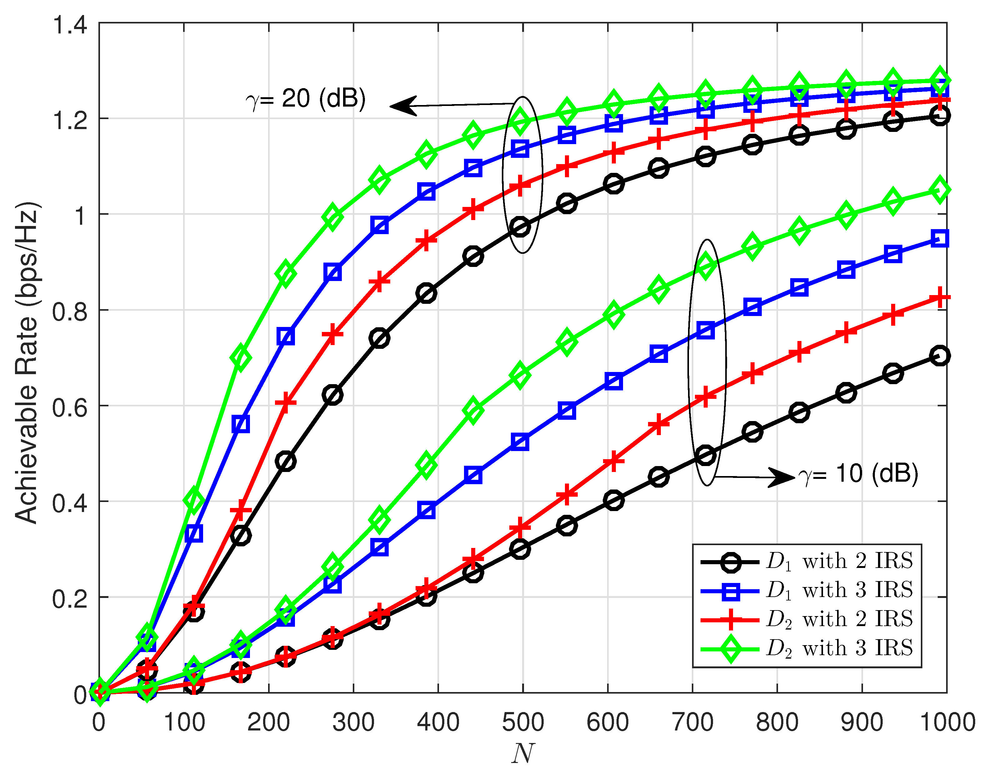
Figure 3 demonstrates the ergodic capacity performance as a function of N and $\gamma$ for two scenarios. When the IRS elements give additional constructive paths, an enhancement in the SNDR could be affected by the increasing N. It is intuitively seen that a higher average SNR at the source leads to a remarkable gap between the ergodic capacity of the two scenarios.

In Figure 4, we confirm the impact of the power allocation factors on the achievable rate. It can be easily seen that more power ${\chi }_1$ assigned to the first user results in a higher achievable rate while the performance of the second user increases at ${\chi }_1=0.65$ for the case of $\gamma$ = 20 (dB) and declines remarkably afterward. The number of meta-surfaces in the three-IRSs case plays an important role in enhancing the quality of received signals at destinations. However, more power assigned to the transmit signal to a selected user is a key factor affecting the achievable rate. On the other hand, we can observe that more IRSs served for user $D_1$ can be employed to improve the rate performance significantly if ${\chi }_1=0.65$ is greater than 0.7.

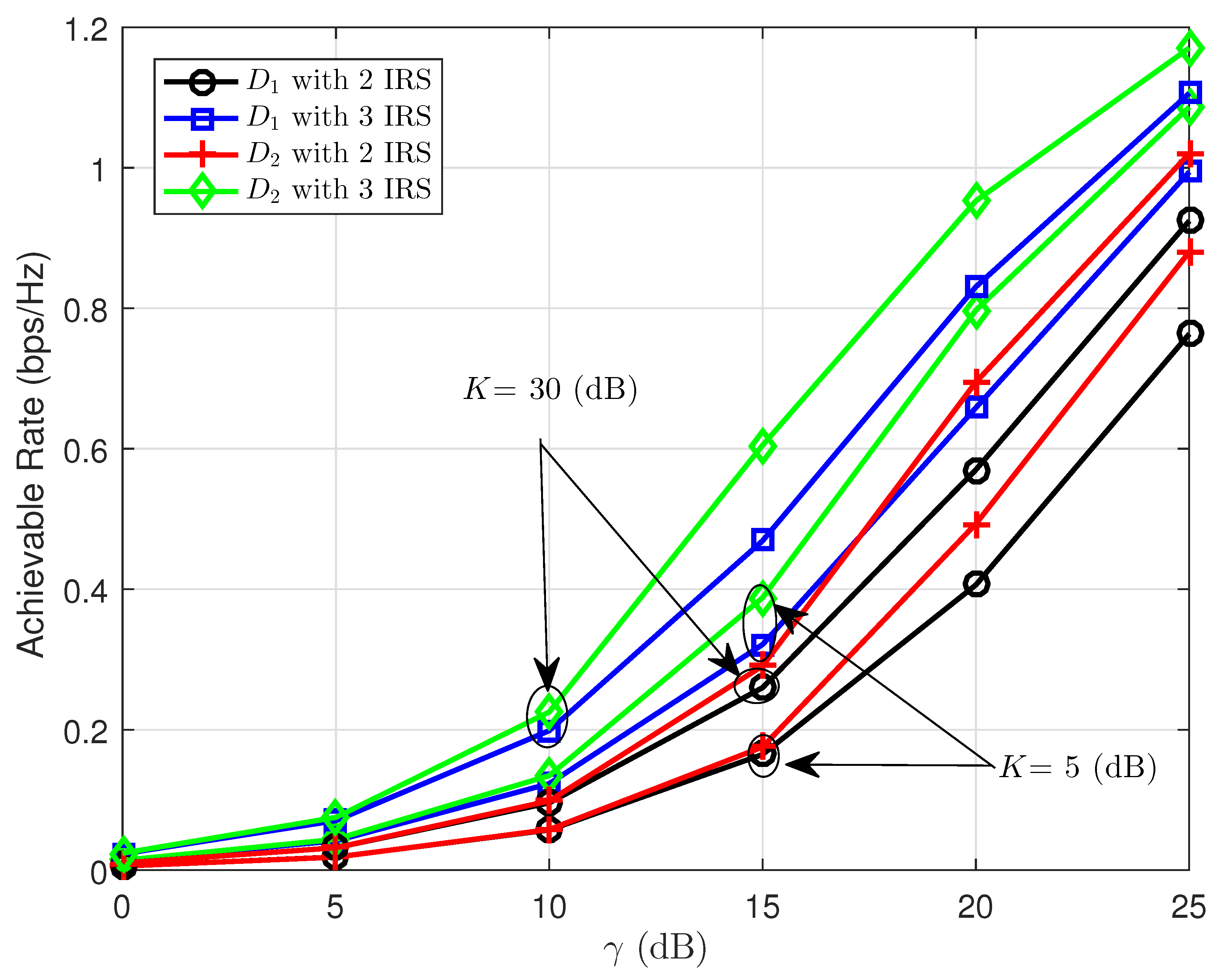
Furthermore, Figure 5 showcases the severity of the hardware impairment for ergodic performance. In particular, due to the transceiver hardware impairment ${\mathrm{{\rm Y}}}_S={\mathrm{{\rm Y}}}_{D_1}={\mathrm{{\rm Y}}}_{D_2}$, the ergodic performance saturates for the case of ${\mathrm{{\rm Y}}}_S={\mathrm{{\rm Y}}}_{D_1}={\mathrm{{\rm Y}}}_{D_2}=0.5$ and cannot be further improved even when increasing $\gamma$ over 30 (dB). It is observed at the low region of $\gamma$ that different levels of transceiver hardware impairment lead to a small gap of achievable rates, and the performance gap among two users is small as well. The capacity ceiling of both users exists when ${\mathrm{{\rm Y}}}_S={\mathrm{{\rm Y}}}_{D_1}={\mathrm{{\rm Y}}}_{D_2}=0.5$ corresponding to $\gamma$ = 30 (dB). It is strongly confirmed that the capacity ceiling is determined by the levels of transceiver hardware impairment rather than N, $\gamma$ and other scenarios.

Figure 6 considers the distances of the source–IRS and IRS–destination links. If IRS is placed at the middle point between the source and destinations, the curves of the achievable rate exhibit the lowest values. When the IRS moves close to either the source or the destinations, the achievable rate improves significantly for the case of $\alpha =2.5$. In this experiment, the achievable rate of the three-IRSs case is still better than the other case.

We can verify how the setting of IRS affects the achievable rate, as shown in Figure 7. At the value of the number of meta-surface $N=400$, the achievable rate obtains the maximum value. The gap among two cases of ${\chi }_1$ could be larger when N is greater than 150. The important conclusion is that it is not necessary to design too many meta-surfaces at the IRS since the achievable rate saturates in the region where N is greater than 500.

The setting of the channel has slight impacts on the ergodic performance since we see a small gap among the curves in Figure 8. Besides the locations of IRS, the quality of the channel gives slight variations in the performance of IoT users. Our similar result in the double-IRS and three-IRSs cases can be compared with the results in the recent work [30]. This means that low-cost IoT can obtain benefits with the double-IRS approach with little influence from selecting the channel models.

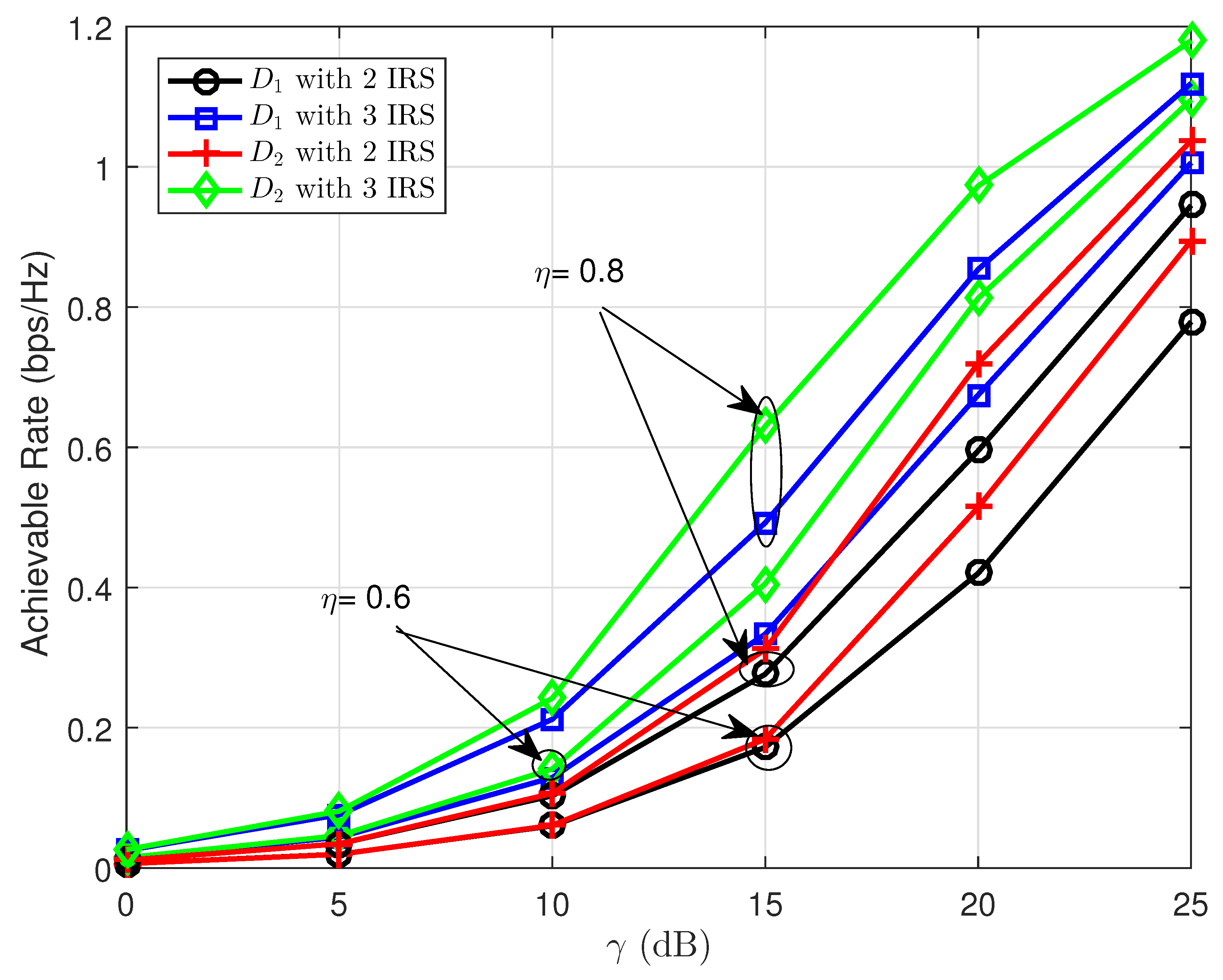
The setting of IRS, i.e., the reflection coefficient, has the main effect on the achievable rates for two cases of IRS, as shown in Figure 9. We can see that $\eta =0.8$ corresponds to a higher achievable rate. The reason is that reflecting the capability of IRS could be better for the case of $\eta =0.8$, and SNDR can be enhanced along with a corresponding improvement of the achievable rate. This simulation still confirms that the three-IRSs case provides higher ergodic performance. However, increasing IRSs leads to a higher cost of deployment. Similarly, Figure 10 confirms that there is a little influence of Rayleigh and Rician channels on ergodic performance for both IoT users.

The benefit of NOMA regarding spectrum efficiency leads to improved performance in terms of the achievable rate, as shown in Figure 11. When the region of $\gamma$ is higher than 20 (dB), a bigger gap between NOMA–IRS and OMA–IRS can be reported. The cases of Rayleigh fading and Rician fading do not affect how much OMA–IRS outperforms OMA–IRS.

5. Conclusions

In this paper, we have recommended the deployment of a double-IRS NOMA–UAV for IoT downlink, since this approach is sufficient to improve performance at destinations. The achievable rates for many scenarios are evaluated carefully to indicate the main impacts under the limitation of imperfect hardware. In contrast to the existing contributions on NOMA transmission design, this paper focused on analytical analysis by characterizing ergodic performance under several channel distributions. The approximate expressions of the achievable rate were verified precisely since these results are similar to those reported in recent work. We provided extensive numerical results of achievable rates with varying hardware impairment levels, power allocation coefficients and channel parameters to validate the accuracy of our derived results. Better ergodic performance can be obtained when the locations of IRSs are close to the source or IoT device. We confirmed that the crucial role of the UAV is to extend the coverage of the base station. We can deploy UAVs in smart city applications since UAVs can be easily deployed in cases of dense devices, buildings and vehicles in cities. In future work, we plan to deal with multiple antennas equipped at the source with respect to improving the reliable transmission of IoT IRS–NOMA–UAV systems.

References

1. Chu, Z.; Zhu, Z.; Li, X.; Zhou, F.; Zhen, L.; Al-Dhahir, N. Resource Allocation for IRS-Assisted Wireless-Powered FDMA IoT Networks. IEEE Internet Things J. 2022, 9, 8774–8785. [Google Scholar] [CrossRef]
2. Tang, J.; Chen, X.; Zhu, X.; Zhu, F. Dynamic Reallocation Model of Multiple Unmanned Aerial Vehicle Tasks in Emergent Adjustment Scenarios. IEEE Trans. Aerosp. Electron. Syst. 2022, 1–43. [Google Scholar] [CrossRef]
3. Tang, J.; Liu, G.; Pan, Q. A Review on Representative Swarm Intelligence Algorithms for Solving Optimization Problems: Applications and Trends. IEEE/CAA J. Autom. Sin. 2021, 8, 1627–1643. [Google Scholar] [CrossRef]
4. Li, B.; Wu, W.; Li, Y.; Zhao, W. Intelligent Reflecting Surface and Artificial-Noise-Assisted Secure Transmission of MEC System. IEEE Internet Things J. 2022, 9, 11477–11488. [Google Scholar] [CrossRef]
5. Shen, H.; Xu, W.; Gong, S.; He, Z.; Zhao, C. Secrecy rate maximization for intelligent reflecting surface assisted multi-antenna communications. IEEE Commun. Lett. 2019, 23, 1488–1492. [Google Scholar] [CrossRef] [Green Version]
6. Zhou, G.; Pan, C.; Ren, H.; Wang, K.; Nallanathan, A. A framework of robust transmission design for IRS-aided MISO communications with imperfect cascaded channels. IEEE Trans. Signal Process. 2020, 68, 5092–5106. [Google Scholar] [CrossRef]
7. Pang, X.; Zhao, N.; Tang, J.; Wu, C.; Niyato, D.; Wong, K.K. IRS-Assisted Secure UAV Transmission via Joint Trajectory and Beamforming Design. IEEE Trans. Commun. 2022, 70, 1140–1152. [Google Scholar] [CrossRef]
8. Feng, K.; Wang, Q.; Li, X.; Wen, C.K. Deep Reinforcement Learning Based Intelligent Reflecting Surface Optimization for MISO Communication Systems. IEEE Wirel. Commun. Lett. 2020, 9, 745–749. [Google Scholar] [CrossRef]
9. Wu, Q.; Zhang, R. Towards Smart and Reconfigurable Environment: Intelligent Reflecting Surface Aided Wireless Network. IEEE Commun. Mag. 2020, 58, 106–112. [Google Scholar] [CrossRef] [Green Version]
10. Do, D.-T.; Le, A.-T. NOMA based Cognitive Relaying: Transceiver Hardware Impairments, Relay Selection Policies and Outage Performance Comparison. Comput. Commun. 2019, 146, 144–154. [Google Scholar] [CrossRef]
11. Do, D.-T.; Van Nguyen, M.-S. Device-to-device transmission modes in NOMA network with and without Wireless Power Transfer. Comput. Commun. 2019, 139, 67–77. [Google Scholar] [CrossRef]
12. Dai, L.; Wang, B.; Yuan, Y.; Han, S.; Chih-lin, I.; Wang, Z. Non-orthogonal multiple access for 5G: Solutions, challenges, opportunities, and future research trends. IEEE Commun. Mag. 2015, 53, 74–81. [Google Scholar] [CrossRef]
13. Van Nguyen, M.S.; Do, D.T.; Al-Rubaye, S.; Mumtaz, S.; Al-Dulaimi, A.; Dobre, O. Exploiting Impacts of Antenna Selection and Energy Harvesting for Massive Network Connectivity. IEEE Trans. Commun. 2021, 69, 7587–7602. [Google Scholar] [CrossRef]
14. Do, D.T.; Le, A.T.; Liu, Y.; Jamalipour, A. User Grouping and Energy Harvesting in UAV-NOMA System with AF/DF Relaying. IEEE Trans. Veh. Technol. 2021, 70, 11855–11868. [Google Scholar] [CrossRef]
15. Do, D.T.; Van Nguyen, M.S.; Voznak, M.; Kwasinski, A.; de Souza, J.N. Performance Analysis of Clustering Car-Following V2X System With Wireless Power Transfer and Massive Connections. IEEE Internet Things J. 2022, 9, 14610–14628. [Google Scholar] [CrossRef]
16. Sun, Z.; Jing, Y. On the Performance of Multi-Antenna IRS-Assisted NOMA Networks With Continuous and Discrete IRS Phase Shifting. IEEE Trans. Wirel. Commun. 2022, 21, 3012–3023. [Google Scholar] [CrossRef]
17. Li, Z.; Chen, W.; Wu, Q.; Wang, K.; Li, J. Joint Beamforming Design and Power Splitting Optimization in IRS-Assisted SWIPT NOMA Networks. IEEE Trans. Wirel. Commun. 2022, 21, 2019–2033. [Google Scholar] [CrossRef]
18. Zhang, X.; Zhang, H.; Du, W.; Long, K.; Nallanathan, A. IRS Empowered UAV Wireless Communication with Resource Allocation, Reflecting Design and Trajectory Optimization. IEEE Trans. Wirel. Commun. 2022, 21, 7867–7880. [Google Scholar] [CrossRef]
19. Ding, Z.; Poor, H.V. A simple design of IRS-NOMA transmission. IEEE Commun. Lett. 2020, 24, 1119–1123. [Google Scholar] [CrossRef] [Green Version]
20. Ding, Z.; Schober, R.; Poor, H.V. On the impact of phase shifting designs on IRS-NOMA. IEEE Wirel. Commun. Lett. 2020, 9, 1596–1600. [Google Scholar] [CrossRef]
21. Zhu, J.; Huang, Y.; Wang, J.; Navaie, K.; Ding, Z. Power Efficient IRS-Assisted NOMA. IEEE Trans. Commun. 2021, 69, 900–913. [Google Scholar] [CrossRef]
22. Fu, M.; Zhou, Y.; Shi, Y. Intelligent Reflecting Surface for Downlink Non-Orthogonal Multiple Access Networks. In Proceedings of the IEEE Globecom Workshops (GC Wkshps), Waikoloa, HI, USA, 9–13 December 2019; pp. 1–6. [Google Scholar]
23. Yang, G.; Xu, X.; Liang, Y.C. Intelligent Reflecting Surface Assisted Non-Orthogonal Multiple Access. In Proceedings of the IEEE Wireless Communications and Networking Conference (WCNC), Seoul, Korea, 25–28 May 2020; pp. 1–6. [Google Scholar]
24. Mu, X.; Liu, Y.; Guo, L.; Lin, J.; Al-Dhahir, N. Exploiting Intelligent Reflecting Surfaces in NOMA Networks: Joint Beamforming Optimization. IEEE Trans. Wirel. Commun. 2020, 19, 6884–6898. [Google Scholar] [CrossRef]
25. Hou, T.; Liu, Y.; Song, Z.; Sun, X.; Chen, Y.; Hanzo, L. Reconfigurable Intelligent Surface Aided NOMA Networks. IEEE J. Sel. Areas Commun. 2020, 38, 2575–2588. [Google Scholar] [CrossRef]
26. Singh, S.K.; Agrawal, K.; Singh, K.; Li, C.P.; Ding, Z. NOMA Enhanced Hybrid RIS-UAV-Assisted Full-Duplex Communication System With Imperfect SIC and CSI. IEEE Trans. Commun. 2022, 70, 7609–7627. [Google Scholar] [CrossRef]
27. Gan, X.; Zhong, C.; Huang, C.; Zhang, Z. RIS-Assisted Multi-User MISO Communications Exploiting Statistical CSI. IEEE Trans. Commun. 2021, 69, 6781–6792. [Google Scholar] [CrossRef]
28. Zhang, Y.; Zhang, J.; Di Renzo, M.; Xiao, H.; Ai, B. Reconfigurable Intelligent Surfaces With Outdated Channel State Information: Centralized vs. Distributed Deployments. IEEE Trans. Commun. 2022, 70, 2742–2756. [Google Scholar] [CrossRef]
29. Selimis, D.; Peppas, K.P.; Alexandropoulos, G.C.; Lazarakis, F.I. On the Performance Analysis of RIS-Empowered Communications Over Nakagami-m Fading. IEEE Commun. Lett. 2021, 25, 2191–2195. [Google Scholar] [CrossRef]
30. Sun, Q.; Qian, P.; Duan, W.; Zhang, J.; Wang, J.; Wong, K.K. Ergodic Rate Analysis and IRS Configuration for Multi-IRS Dual-Hop DF Relaying Systems. IEEE Commun. Lett. 2021, 25, 3224–3228. [Google Scholar] [CrossRef]
31. Ren, H.; Wang, K.; Pan, C. Intelligent Reflecting Surface-Aided URLLC in a Factory Automation Scenario. IEEE Trans. Commun. 2022, 70, 707–723. [Google Scholar] [CrossRef]
32. Xing, Z.; Wang, R.; Wu, J.; Liu, E. Achievable Rate Analysis and Phase Shift Optimization on Intelligent Reflecting Surface With Hardware Impairments. IEEE Trans. Wirel. Commun. 2021, 20, 5514–5530. [Google Scholar] [CrossRef]
33. Tran, P.T.; Nguyen, B.C.; Hoang, T.M.; Nguyen, T.N. On Performance of Low-Power Wide-Area Networks with the Combining of Reconfigurable Intelligent Surfaces and Relay. In IEEE Transactions on Mobile Computing; IEEE: Piscataway, NJ, USA, 2022. [Google Scholar]
34. Yue, X.; Liu, Y.; Kang, S.; Nallanathan, A.; Ding, Z. Exploiting Full/Half-Duplex User Relaying in NOMA Systems. IEEE Trans. Commun. 2018, 66, 560–575. [Google Scholar] [CrossRef] [Green Version]
35. Yang, L.; Yang, Y.; Hasna, M.O.; Alouini, M.S. Coverage, Probability of SNR Gain, and DOR Analysis of RIS-Aided Communication Systems. IEEE Wirel. Commun. Lett. 2020, 9, 1268–1272. [Google Scholar] [CrossRef]
36. Abdullah, Z.; Chen, G.; Lambotharan, S.; Chambers, J.A. A Hybrid Relay and Intelligent Reflecting Surface Network and Its Ergodic Performance Analysis. IEEE Wirel. Commun. Lett. 2020, 9, 1653–1657. [Google Scholar] [CrossRef]
Figure 1. The IRS–NOMA–UAV system model with source, two IRSs and ground users.
Drones 06 00408 g001
Figure 2. The flowchart of Monte Carlo simulations.
Drones 06 00408 g002
Figure 3. The performance of overall achievable rates by varying the number of IRSs (N = N 1 = N 2 = N 3 ) when changing γ with Rayleigh fading.
Drones 06 00408 g003
Figure 4. Impact of power allocation factors χ 1 on overall achievable rates by varying γ with Rayleigh fading.
Drones 06 00408 g004
Figure 5. Impact of hardware impairments Υ S = Υ D 1 = Υ D 2 on overall achievable rates by varying γ with Rayleigh fading.
Drones 06 00408 g005
Figure 6. Impact on the performance of overall achievable rates by varying x I 1 = x I 2 = x I 3 when changing α with Rayleigh fading.
Drones 06 00408 g006
Figure 7. The achievable rates versus N = N 1 = N 2 = N 3 when changing χ 1 with Rician fading.
Drones 06 00408 g007
Figure 8. Impact on the performance of overall achievable rates by varying γ when changing the Rician-K factor.
Drones 06 00408 g008
Figure 9. Impact on the performance of overall achievable rates by varying γ when changing η with Rician fading.
Drones 06 00408 g009
Figure 10. Impact on the performance of overall achievable rates of Rayleigh fading and Rician fading by varying γ .
Drones 06 00408 g010
Figure 11. Impact on the performance of overall achievable rates of Rayleigh fading and Rician fading between NOMA and OMA with two IRSs by varying γ .
Drones 06 00408 g011
Publisher’s Note: MDPI stays neutral with regard to jurisdictional claims in published maps and institutional affiliations.