Simulating a Hybrid Acquisition System for UAV Platforms

Abstract

Currently, there is a rapid trend in the production of airborne sensors consisting of multi-view cameras or hybrid sensors, i.e., a LiDAR scanner coupled with one or multiple cameras to enrich the data acquisition in terms of colors, texture, completeness of coverage, accuracy, etc. However, the current UAV hybrid systems are mainly equipped with a single camera that will not be sufficient to view the facades of buildings or other complex objects without having double flight paths with a defined oblique angle. This entails extensive flight planning, acquisition duration, extra costs, and data handling. In this paper, a multi-view camera system which is similar to the conventional Maltese cross configurations used in the standard aerial oblique camera systems is simulated. This proposed camera system is integrated with a multi-beam LiDAR to build an efficient UAV hybrid system. To design the low-cost UAV hybrid system, two types of cameras are investigated and proposed, namely the MAPIR Survey and the SenseFly SODA, integrated with a multi-beam digital Ouster OS1-32 LiDAR sensor. Two simulated UAV flight experiments are created with a dedicated methodology and processed with photogrammetric methods. The results show that with a flight speed of 5 m/s and an image overlap of 80/80, an average density of up to 1500 pts/m² can be achieved with adequate facade coverage in one-pass flight strips.

1. Introduction

Unmanned aerial vehicles (UAV) are becoming increasingly popular, making them an important tool for remote sensing applications [1,2,3,4,5,6,7]. This includes regular data collection for indoor 3D mapping [8], natural hazards [9], topo-bathymetry [10,11], air pollution monitoring [12,13], management of urban areas [14], etc.

The primary benefit of UAV platforms over conventional acquisition strategies is their affordability and flexibility. According to the demands of the user, flexibility refers to the ability to quickly adjust to various operational situations. Depending on the scope of the problem and the application type, quite different solutions may be used. On the other hand, cost-effective UAVs may accommodate any budget, from low-cost consumer solutions to extremely pricey ones that include high-end sensors. This explains quite clearly why UAVs have made (3D) mapping more accessible in many underdeveloped nations [15,16] or why they are being used to monitor critical areas such as glaciers [17], mines [18], electrical lines [19], and other man-built infrastructures [20].

The range of applications for employing UAV platforms for monitoring dynamic and complex environments has recently increased thanks to the proliferation of platforms on the market, the additional onboard devices, the faster and more reliable communication methods, and the improved battery life. The next generation of UAV applications is quickly approaching because of the advancement in real-time onboard processing [21] and the development of autonomous and dependable systems [22].

Multi-sensor data integration is the newest development in terrestrial and aerial 3D mapping applications, in addition to conventional imaging (passive) and range (active) sensors. The rapidly expanding market for hybrid mapping systems, which combine complementing range and image sensors on a single (mobile) platform, serves as an example of this. Rapidly expanding hybrid sensor technologies are entering the topographic and urban aerial mapping markets, creating new possibilities for higher-quality geospatial products [23]. According to this viewpoint, the simultaneous capture of the oblique images and LiDAR data appears to have the capacity to significantly advance the field of aerial (urban) mapping [24].

In fact, in recent years both aerial LiDAR (Light Detection and Ranging) and photogrammetry have developed into cutting-edge methods for obtaining 3D-enriched geospatial information products. Now, the prospective next step is to jointly leverage their individual benefits into a unique “hybrid” system [25]. On the one hand, airborne LiDAR offers very reliable terrain elevation information and multi-objective capabilities, allowing for the acquisition and modeling of the bare ground while penetrating vegetation. Due to these advantages, ALS (airborne laser scanning) has emerged as the most advanced mapping technique for the automated production of building models, 2.5D point clouds, and digital terrain models [26,27]. On the other hand, improvements in photogrammetry and computer vision, notably those connected to the creation of novel dense image matching (DIM) techniques [28,29], have increased automation in the image-based 3D reconstruction of a scene, with the intention of producing high-resolution DSMs (digital surface models). Nowadays, point clouds created from images can have a spatial resolution equal to the GSD (ground sample distance) of the source imagery and an ideal accuracy less than the GSD level, provided that there is adequate redundancy and a sufficient geometrical structure of the image rays. Additionally, the inclusion of oblique photos in the block enhances the overall dense matching quality [30]. In fact, the rapidly developing field of airborne oblique photogrammetry [31] has advanced geometric processing toward “true” 3D space, enabling more thorough and accurate extraction of information in urban scenes [28,32,33,34].

While multi-view cameras for UAV platforms have also started to be commercially accessible for UAV platforms (

Table 1. Specifications of some commercial multi-view camera systems for UAV platforms.

	Resolution	Sensors	Size	Weight
Viewprouav VO305	305 MPx	Full frame	20 m × 20 m × 112 mm	-
Share 303S Pro	305 MPx	Full frame	200 × 200 × 125 mm	1.4 kg
DroneBase N5	120 MPx	APS-C	160 × 160 × 85 mm	730 gr
ADTi Surveyor 5 PRO	120 MPx	APS-C	105 × 150 × 80 mm	850 gr
Quantum-System D2M	130 MPx	APS-C	-	830 gr
JOUAV CA504R	305 MPx	Full frame	270 × 180 × 154 mm	2.25 kg

, Figure 1), the availability of hybrid sensors for UAVs is still rare.

Paper Aims

The paper proposes and validates, through simulations, a UAV hybrid sensor composed of five RGB cameras coupled with a LiDAR sensor for 3D mapping purposes. In particular, the innovative aspects include:

-

a novel (simulated) low-cost, low-weight, hybrid, multi-view hybrid acquisition system for UAV platforms (Section 2.1, Section 2.2 and Section 2.3);

-

dedicated software for UAV flight planning with a hybrid sensor (Section 2.4);

-

experiments with simulated data on two large urban scenarios (Section 3).

The remainder of the paper is organized as follows: Section 2 reports the proposed hybrid system for 3D mapping applications with UAV platforms, including a flight planning tool. Section 3 presents the experiments on and the analyses of two different simulated scenarios. Section 4 provides a critical discussion of the proposed hybrid sensor, and Section 5 concludes the paper.

2. Proposed Hybrid System for UAV Platforms

The simulated hybrid acquisition system for UAV platforms is composed of multiple cameras and a LiDAR. The investigation does not tackle any GNSS/IMU sensors, but the proposed hybrid system could be combined with any positioning sensor for direct georeferencing [35,36,37] or RTK/PPP processing [38,39,40] purposes.

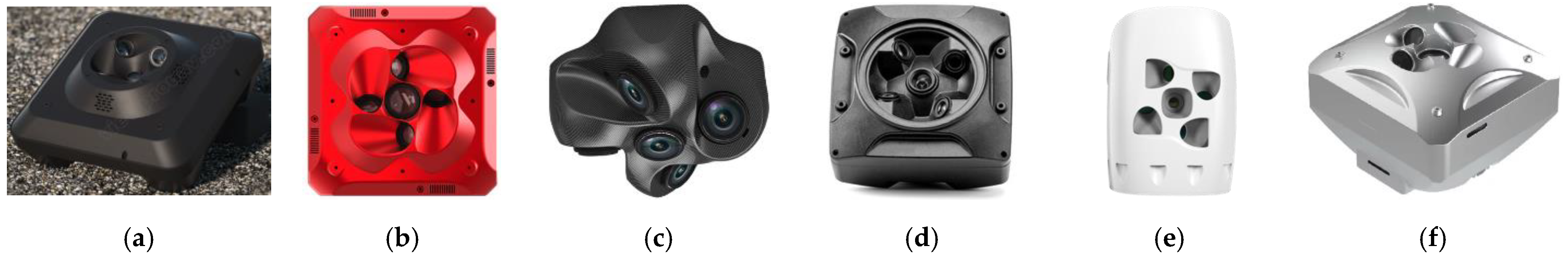
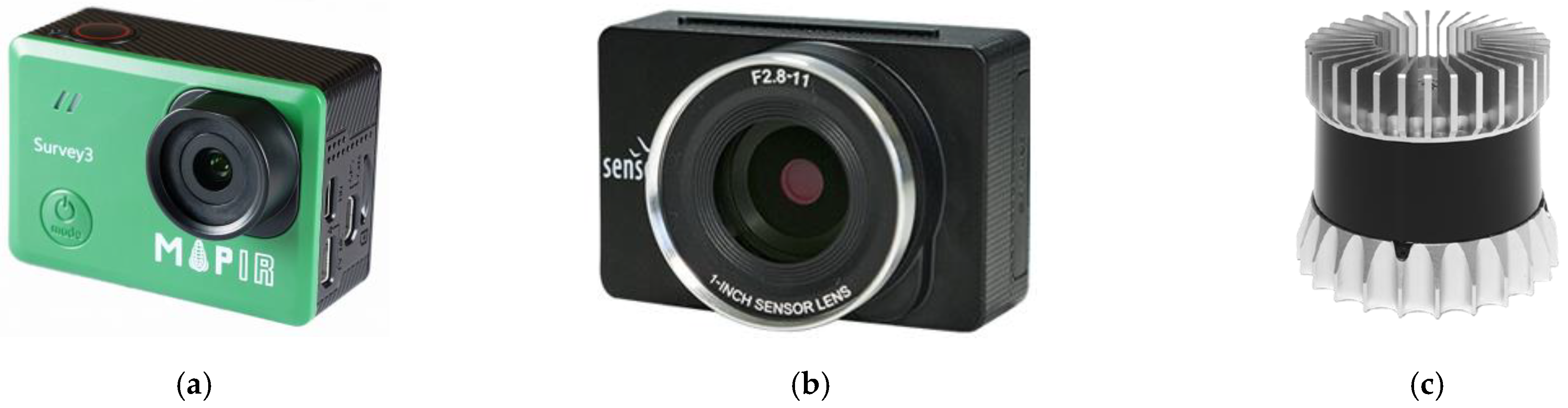
2.1. The Camera Components

Among the suitable RGB imaging devices, considering their (camera body and sensor) size, weight, resolution, and prices, the following were selected (

Table 2. Main characteristics of the considered MAPIR and senseFly cameras.

Specification	MAPIR Survey3W	senseFly SODA
Focal length [mm]	8.25	10.6
Sensor [pixels]	Sony Exmor R IMX1174032 × 3024	CMOS 1”, 5472 × 3648
Pixel size [microns]	1.55	2.33
Field of view	87°	74°
Storage [GB]	Max 128 GB Storage	Based on external memory
Data exchange format	PWM, USB, HDMI, and SD	PWM, USB, HDMI, and SD
Shutter speed	Global Shutter 1/2000 to 1 min	Global Shutter 1/500–1/2000 s
Aperture	f/2.8	f/2.8–f/11
Dimensions	59 × 41.5 × 36 mm	75 × 48 × 33 mm
Weight	75.4 g with battery	85 g
Battery	1200 mAh Li-Ion (150 min)	No internal battery, powered by drone
Price	ca. EUR 400	ca. EUR 1500

, Figure 2): a MAPIR Survey3 [41] and a senseFly SODA [42]. They both fulfilled the planned characteristics and were constrained to realize a low-cost, low-weight, multi-view imaging system for UAV platforms.

2.2. The LiDAR Component

The second type of sensor in the proposed UAV hybrid system is LiDAR. Among a variety of available LiDAR sensors, it was decided to select a multi-beam LiDAR to guarantee a high coverage and density of points, a reasonable weight, an effective scanning range, and acceptable accuracy limits to keep the proposed hybrid system at a lower cost. Following the in-depth analyses of [43], the Ouster OS1-32 LiDAR sensor was chosen. The scanning sensor is a suitable candidate because of its higher productivity using 32 scanning beams, the symmetric and wide field of view above/below the horizontal plane, and the half weight of other similar sensors and, most importantly, because it is a digital LiDAR (single-photon avalanche diode) [44]. This characteristic gives the advantage of having an array scanning pattern (image alike) which enables the application of the image processing techniques. Compared to the analogue-type LiDARs, no more calibration is required, and more advantages will be gained, such as less sensitivity to temperature, smaller size, and a higher data rate. Furthermore, the Ouster LiDAR already has an IMU of InvenSense ICM-20948 included. The main specifications of the Ouster OS1-32 LiDAR are shown in

Table 3. Main characteristics of the Ouster OS1-32 LiDAR sensor and its typical scanning ground footprint (right).

LiDAR Sensor/System	Ouster OS1-32
Max. Range	≤120 m@80% reflectivity
Typical Range Accuracy 1σ	±3 cm
Beam divergence	0.18° (3 mrad)
Beam footprint	22 cm@100 m
Scanning channels/beams	32 channels
Output rate pts/sec.	655,360
Laser Returns	1 per outgoing pulse
FOV-Vertical	45° (±22.5°)
Rotation rate	10–20 Hz
Angular resolution	0.35°–2.8°
LiDAR mechanism	Spinning
LiDAR type	Digital
Laser Wavelength	865 nm
Power consumption	14–20 w
Weight	455 g
Dimensions (diameter × height)	85 × 73.5 mm
Operating Temperature	−20 °C to +50 °C
Initial price	ca. EUR 8000

.

Another multi-beam LiDAR that could be used in the suggested hybrid system is the Quanergy M8 type, investigated in [43]. This LiDAR sweeps eight beams at a frequency ranging from 5 to 20 Hz and offers a scanning range of 100 m@ 80% object reflectivity. However, it has a 900 g weight, which should also be considered in order to not affect the UAV payload.

2.3. The Integrated Hybrid System

The assembled hybrid system is shown in Figure 3, and its overall specifications are given in

Table 4. Overall characteristics of the integrated camera and LiDAR sensors.

LiDAR	Ouster S1-32
Number of cameras	4 oblique + 1 nadir
Dimensions	24.6 cm × 21 cm × 8 cm (MAPIR config.) 23.4 cm × 15.8 cm × 8 cm (SODA config.)
Focal length	10.6 mm (SODA config.) 8.25 mm (MAPIR config.)
Megapixels	12 MPx (MAPIR config.) 20 MPx (SODA config.)
Camera tilting	45° (or 30°)
Data exchange format	USB Memory Stick
Expected operation time per charge	>1 h
Operational temperature range	0 °C to 40 °C
Mass	<1 kg, with battery
Price	EUR <10,000

. Considering that there is a bounding box to host all the sensors, the hybrid system is supposed to weigh less than a kg and operate for up to 1 h. The design of the hybrid system configuration is applied using the open-source tool Blender [5].

The camera system is designed in a Maltese cross configuration, where four cameras are tilted at 45° while the fifth camera is fixed at the nadir view. As the field of view (FOV) of the senseFly is bigger than that of the Survey 3, there will be a larger footprint with some overlap, as shown in Figure 3.

Both configurations, based on the MAPIR and SODA cameras, are designed carefully to guarantee no self-occlusion and to keep the distance between them at a possible minimum. The same applies to the placement of the Ouster LiDAR. The scanning ground footprint of LiDAR is also shown in Table 4.

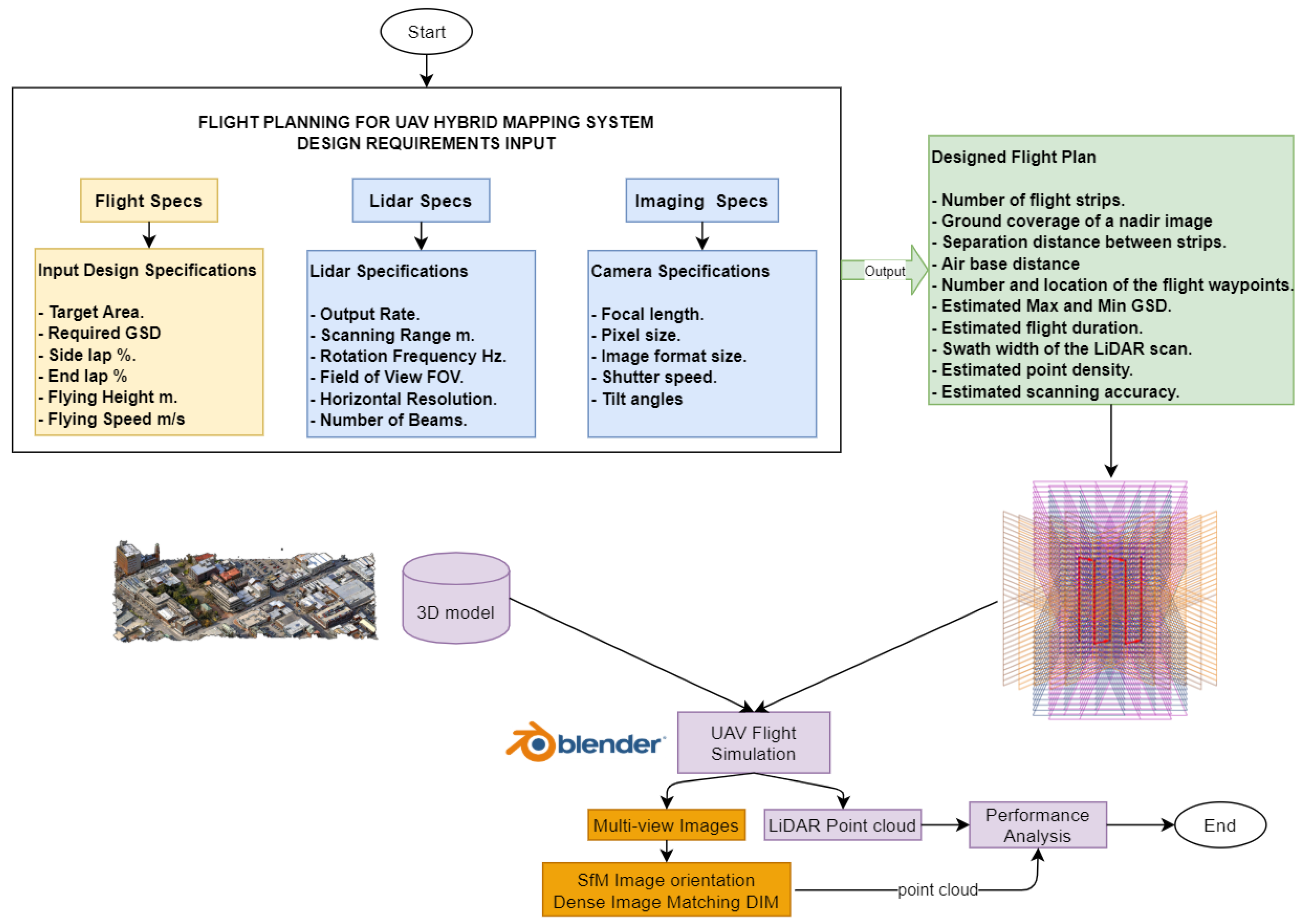
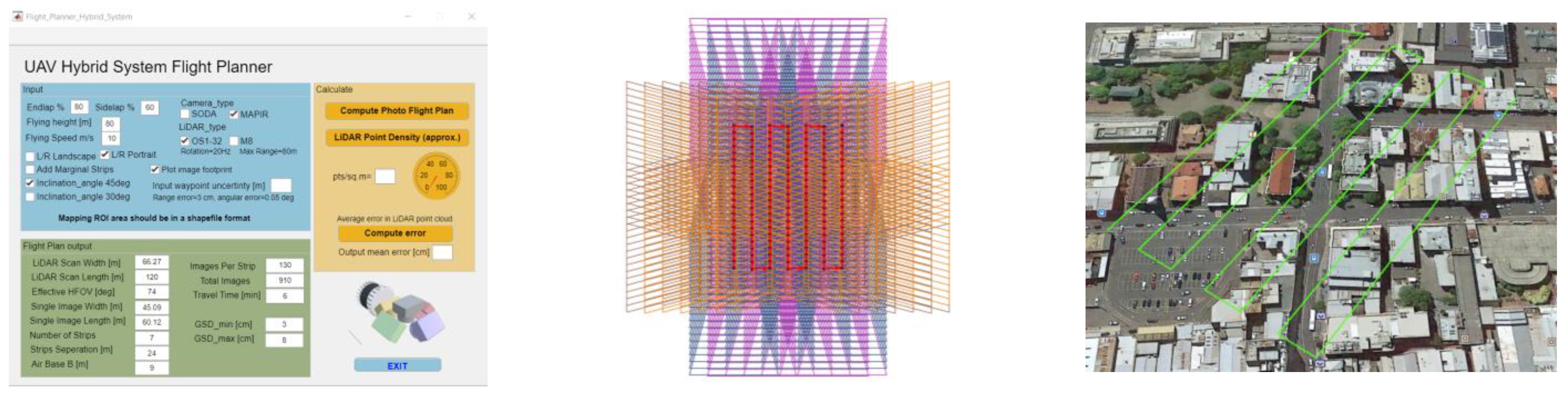
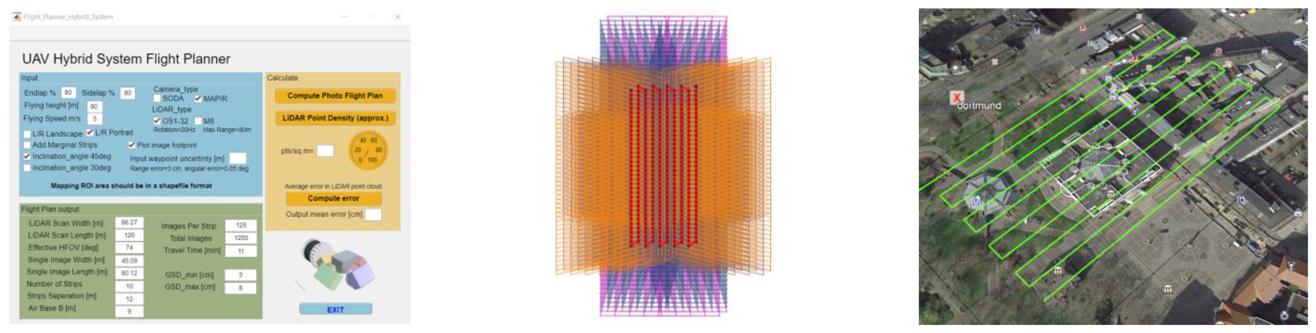
2.4. UAV Flight Planning Tool for Hybrid Systems

A prototype flight planning tool was built using MATLAB 2020 (Figure 4) (Available online: https://github.com/Photogrammtery-Topics/flight-planning-tool-for-Hybrid-UAV-system/wiki (accessed on 18 October 2022)). As with the UAV flight planning tools presented in [43], the calculations are based on the selected flying altitude, flying speed, overlap percentages, and camera settings. Furthermore, the area of interest is defined by a polygonal shapefile regardless of its complexity as it will be generalized into a minimum rectangular bounding box. The tool can handle the flight plans of the two proposed hybrid camera systems (either senseFly- or MAPIR-based) with a camera inclination angle of 45° or 30°. The tool can simulate the integration of the Ouster OS1-32 and also that of a Quanergy M8 LiDAR, and it estimates the average point cloud density.

The following output flight plan parameters are calculated:

• The maximum and minimum image GSD;
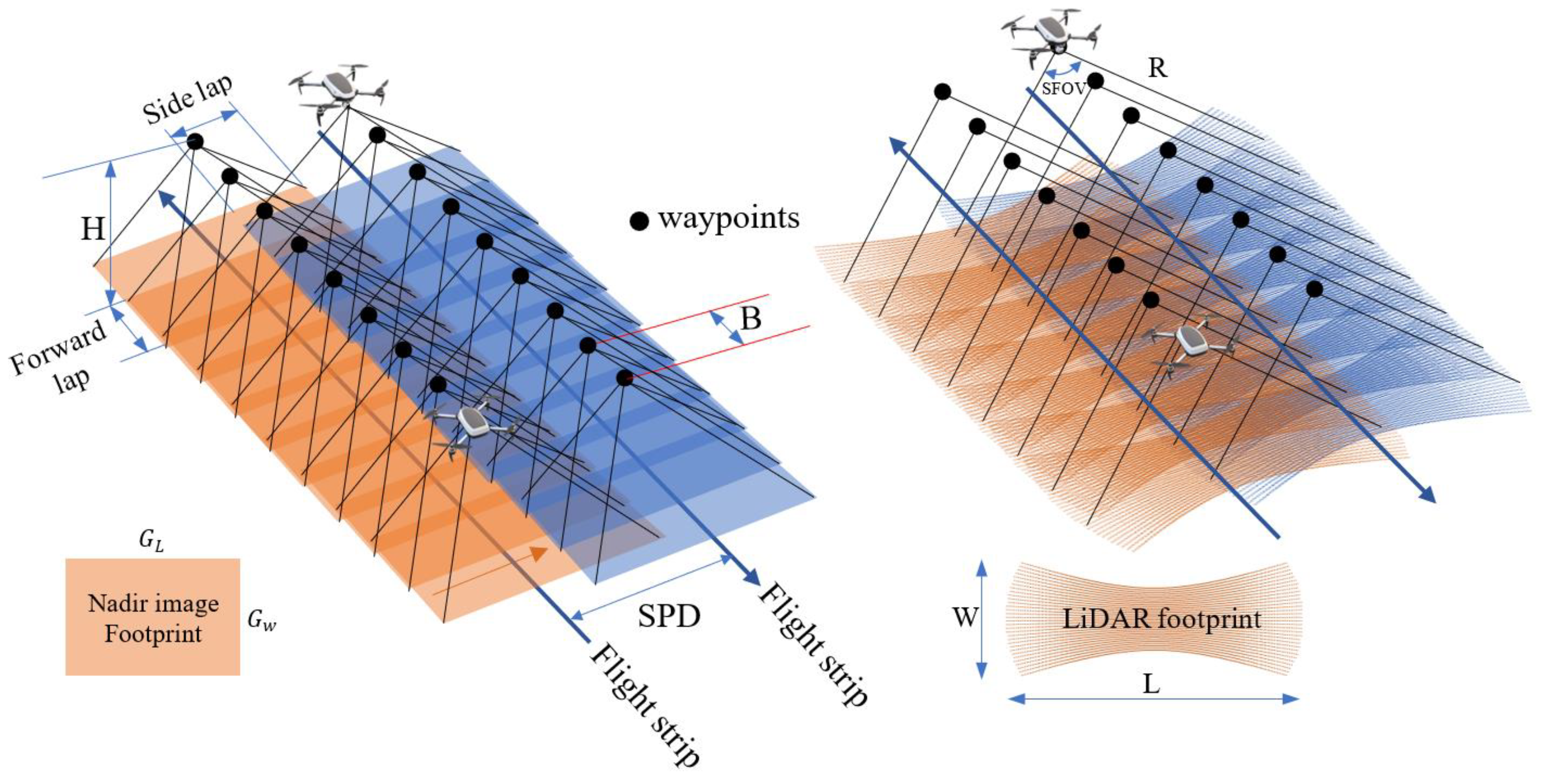
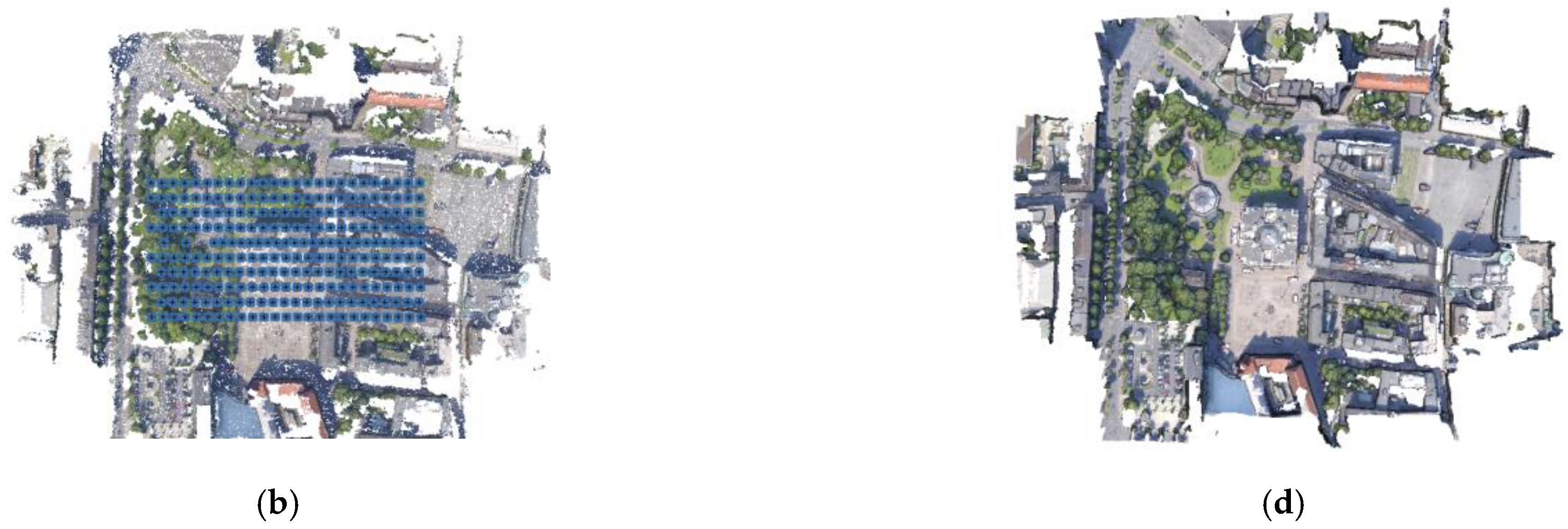
• The ground coverage of the multi-view images (Figure 4b);
• The number of flight strips, waypoints per strip, and the total waypoints;
• The separation distance between the adjacent flight strips;
• The baseline between the two consecutive waypoints;
• The estimated travel time;
• The LiDAR scan footprint width and length;
• The LiDAR effective scanning angles.

The suggested oblique views at 45° will entail an enlargement effect on the GSD values. Accordingly, the $GS{D}_{min}$ and $GS{D}_{max}$ values are computed using the following equations [45]:

$$GS{D}_{min}=pixel.\frac{H}{f} +\frac{cos\left(\beta -t\right)}{cos\beta }$$

(1)

$$GS{D}_{max}=GS{D}_{min}. \frac{cos\left(\beta -t\right)}{cos\beta }$$

(2)

with

• f = focal length,
• H = flying height above the ground level,
• t = inclination angle of the camera,
• β = inclination angle to a certain image point.

The output flight plan parameters are calculated using the following equations [46]:

$$scale no.=\left(\frac{H}{f}\right)$$

(3)

$$G_w=format width\times scale no.$$

(4)

$$G_L=format length\times scale no.$$

(5)

$$B=G_w\left(1-end lap \%\right)$$

(6)

$$SPD=G_L\left(1-side lap \%\right)$$

(7)

$$NFS = round \left(\frac{W_{area}}{SPD}+1\right)$$

(8)

$$N=round \left(\frac{L_{area}}{B}+2\right)$$

(9)

$$Total waypoints=NFS\times N$$

(10)

$$W=2 tan\left(\frac{VFOV}{2}\right).H$$

(11)

$$L =2 \sqrt{\left(R^2-H^2\right)}$$

(12)

$$SFOV=2 ta{n}^{-1}\left(\frac{L/2}{H}\right)$$

(13)

where

• $L_{area}, W_{area}$: project area dimensions are defined as a rectangle with a length $L$ and width $W$.
• $G_w$: nadir image coverage along track.
• $G_L$: nadir image coverage across track.
• $B: airbase$ distance between two successive waypoints.
• $SPD$: separation distance between the flight strips.
• $NFS$: number of flight strips rounded to positive infinity.
• $N:$ number of waypoints per strip.
• $R:$ scanning range of the LiDAR.
• $VFOV$: vertical field of view of the LiDAR.
• $W$: along-track LiDAR scanning width.
• $L$: across-track swath width of the LiDAR scanning.
• $SFOV$: effective scanning field of view.

Figure 5 is shown for a better understanding of the aforementioned flight parameters.

The algorithms to compute the flight planning parameters and the estimated LiDAR point density are shown in

Table 5. Pseudocode for the flight planning parameters.

Input: the ROI shapefile, camera and LiDAR parameters, required GSD. Output: Flight plan parameters including: UAV waypoints and save them as an array in a folder. Display planning results in the tool GUI The plot of the footprints of the images Check input options of the overlap, height, speed, inclination angle, portrait/landscape, type of the camera, and marginal flight strips Compute the min. and max. GSD and display them in the GUI Call the function of the flight planner calculator: Plot the ROI Define if the ROI is either elongated NS or EW Calculate the airbase B, no. of strips, no. of images, travel time, and the XYZ of the waypoints Return

and

Table 6. Pseudocode for the estimation of the LiDAR point cloud on the ground.

Input: The waypoints calculated from the flight planner in Table 1. The LiDAR beams’ angular configuration and parameters. Output: Estimation of the density of LiDAR points Apply the computations: Define the ground object by a horizontal plane (DSM TIN-not applied in the prototype). For each beam j For each scanning station $i$ on the planned path For each scanning beam For each scanning angle [0°—angular resolution—360°] Apply the LiDAR equation using the predefined orientation using polar coordinates azimuth, elevation, and range Check if the calculated scanning ray is intersecting the ground plane Check visibility (in case of a DSM) Save scanning point XYZ Extract the scanning points located inside the ROI Repeat Return

.

The tool also allows users to estimate the LiDAR point cloud average error using the propagation of error calculations and a given waypoint uncertainty [47]. The propagation of errors is useful to estimate one component of the accuracy of the sensor errors by transforming the measured range and angles to the 3D coordinates X_i, Y_i, Z_i, as follows:

$$\begin{array}{c}{X}_{\mathrm{i}}=X_1+R.cos\left(Az\right).cos\left(V\right)\\ Y_{\mathrm{i}}=Y_1+R.sin\left(Az\right).cos\left(V\right)\\ Z_{\mathrm{i}}=Z_1+R.sin\left(V\right)\end{array}$$

(14)

where

• R is the measured range distance from the sensor to the scanned point.
• $Az$ is the measured azimuth angle of the laser beam.
• $V$ is the measured vertical angle of the laser beam measured from the horizontal plane.
• $X_1, Y_1$, and $Z_1$ are the coordinates of the LiDAR at time $t_1$.

An error propagation can be applied to Equation (14) using Jacobian Matrix J to estimate the errors of the scanned points in the point cloud, as follows in Equation (15):

$${{\displaystyle \sum }}_{XYZ}^{}=J{{\displaystyle \sum }}_{R,Az,V}^{}{J}^t=\left[\begin{array}{ccc}{\sigma }_{Xi}{}^2& & cov. \\ & {\sigma }_{Yi}{}^2& \\ cov. & & {\sigma }_{Zi}{}^2\end{array}\right]$$

(15)

where

• ${{\displaystyle \sum }}_{R,Az,V}^{}:$ The variance–covariance matrix of the observed range and angles.
• ${{\displaystyle \sum }}_{XYZ}^{}:$ The variance–covariance matrix of the derived coordinates of point $P$_i where ${\sigma }_{Xi}{}^2, {\sigma }_{Yi}{}^2,$ ${\sigma }_{Zi}{}^2$ represent the variances of the coordinates, respectively.

3. Experiments and Analyses

To test the mapping capability and productivity of the proposed multi-view hybrid system for UAV platforms, two simulated test flights were designed using the Blender open-source tool [48]. For each test, using the simulated flight trajectories (Section 2.4), the multi-view image datasets were rendered in Blender and then imported into Metashape [49] for a bundle block adjustment and dense point cloud generation (Figure 6). In both of the proposed camera systems (Section 2.3), the rendered images are assumed to be distortion-free since they are simulated using ideal camera conditions. Furthermore, to have a robust bundle adjustment with a lower number of blunders, only the tie points viewed in at least three images are kept before optimizing the final orientation parameters. It is worthwhile mentioning that a recommended shutter speed ≥ 1/1250 is considered to have a motion blur ≤ half a pixel. The LiDAR scanning with the Ouster OS1-32 is then applied along the image-based trajectory, assuming a maximum range of 100 m and a low target reflectivity of the scanned objects. The point clouds from each sensor, together with the integrated ones, are finally analyzed in terms of point density.

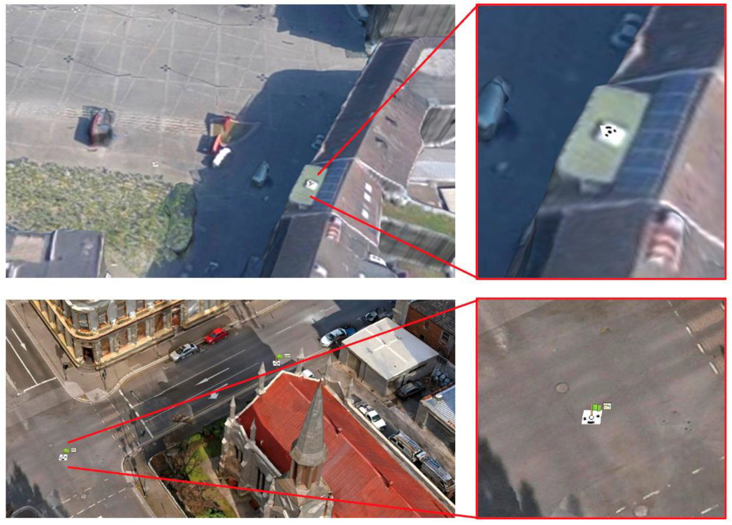
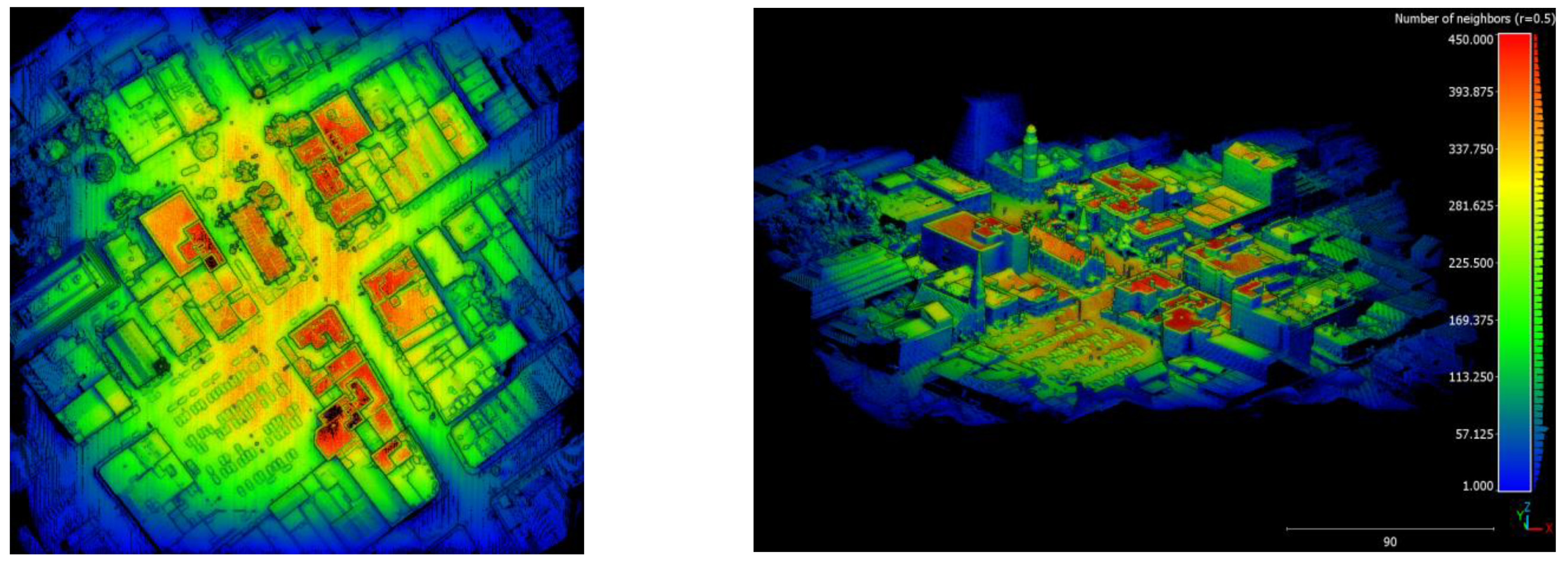
3.1. Use Case #1—Launceston

The first 3D mapping test was simulated over the city of Launceston in Tasmania, where a free 3D model was available [50]. An area of interest (AOI) of 150 by 170 m² was selected and the flight plans were computed using the developed prototype tool described in Section 2.4. The flight input parameters were chosen as follows:

• flying height = 80 m
• flying speed = 10 m/s
• end lap = 80% and side lap = 60%

For a highly accurate georeferencing and accuracy evaluation, five ground control points (GCPs) and seven checkpoints (CPs) were distributed over the study area by placing coded targets which could be automatically marked and measured (Figure 7).

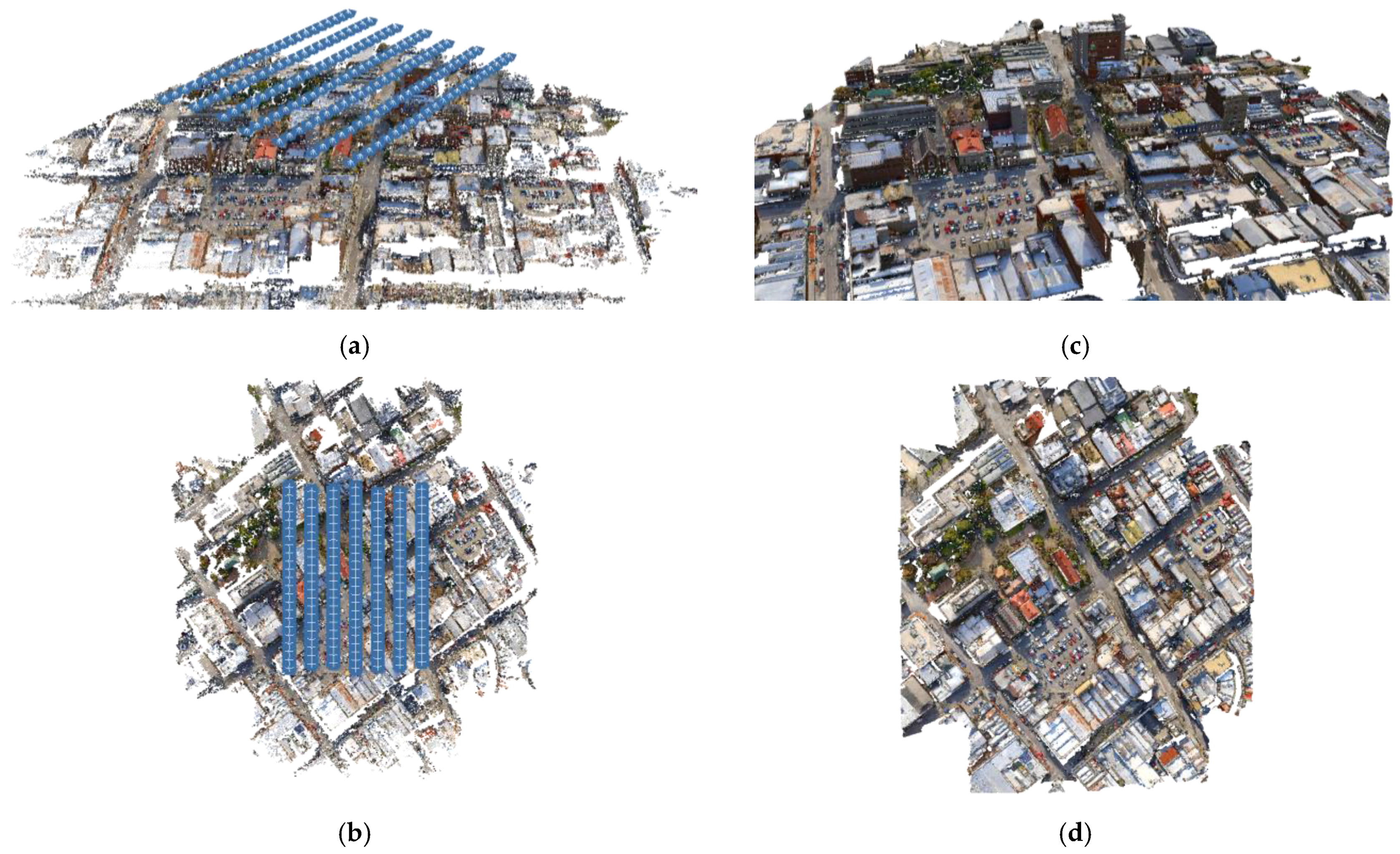
3.1.1. SenseFly-Based Hybrid UAV Surveying

Given the flight input parameters and the camera specifications, the plan was to capture a total of 475 images along five flight strips. The plan was for the flight strips to not be parallel to the streets and buildings in the scene in order to have a better understanding of the results (see also Discussions). The flight strips, footprints of the images, and the flight plan are shown in Figure 8. The GSD of the nadir images is 1.8 cm while the oblique views span from 6 to 22 cm.

The bundle block adjustment processing of the rendered images closed with a reprojection error of 0.75 pixels, a multiplicity of ca. 5, and a sparse point cloud of 421,000 points (Figure 9a,b). The root mean square errors (RMSEs) on the GCPs and CPs are shown in

Table 7. Accuracy analyses on the two simulated image datasets over Launceston and GCP/CP distribution (right).

	RMSE_ XY (mm)	RMSE_Z (mm)	Total RMSE (mm)
	senseFly-based hybrid system (nadir GSD: 1.8 cm)
GCPs (5)	4.1 mm	1.3 mm	4.3 mm
CPs (7)	4.3 mm	1.8 mm	4.6 mm
	MAPIR-based hybrid system (nadir GSD: 1.5 cm)
GCPs (5)	4.4 mm	1.0 mm	4.5 mm
CPs (7)	3.7 mm	1.2 mm	3.8 mm

. A dense point cloud was created afterwards using Dense Image Matching (DIM) methods, resulting in ca. 167 million points (Figure 9c,d).

Following the same five imaging flight strips, the LiDAR scanning simulation was applied using the OS1-32 sensor, with a maximum scanning range of 100 m and a rotation frequency of 20 Hz. The simulated point cloud consists of ca. 15 million points. The density of the point cloud is shown in Figure 10, where the red color indicates ≥200 pts/m².

3.1.2. MAPIR-Based Hybrid UAV Surveying

Using the same AOI and flight planning input parameters and the MAPIR camera specifications, the plan was to capture a total of 910 simulated images along seven overlapping strips (Figure 11). The GSD of the nadir images is 1.5 cm while the oblique views (45 deg inclination) span from 3 to 8 cm.

The photogrammetric processing of the simulated multi-view images produced a reprojection error of 0.73 pixels, with a multiplicity of ca. 5 and a sparse point cloud of 652,815 points (Figure 12a,b). The root mean square errors (RMSEs) on the GCPs and CPs are shown in Table 7. A dense point cloud was created afterwards, resulting in ca. 202 million points (Figure 12c,d).

Following the same seven flight strips planned with the MAPIR multi-view camera system, the LiDAR scanning was applied and a point cloud of ca. 21 million was produced using the OS1-32 scanner. The density of the point cloud was computed and visualized, with the red color indicating ≥200 pts/m² (Figure 13).

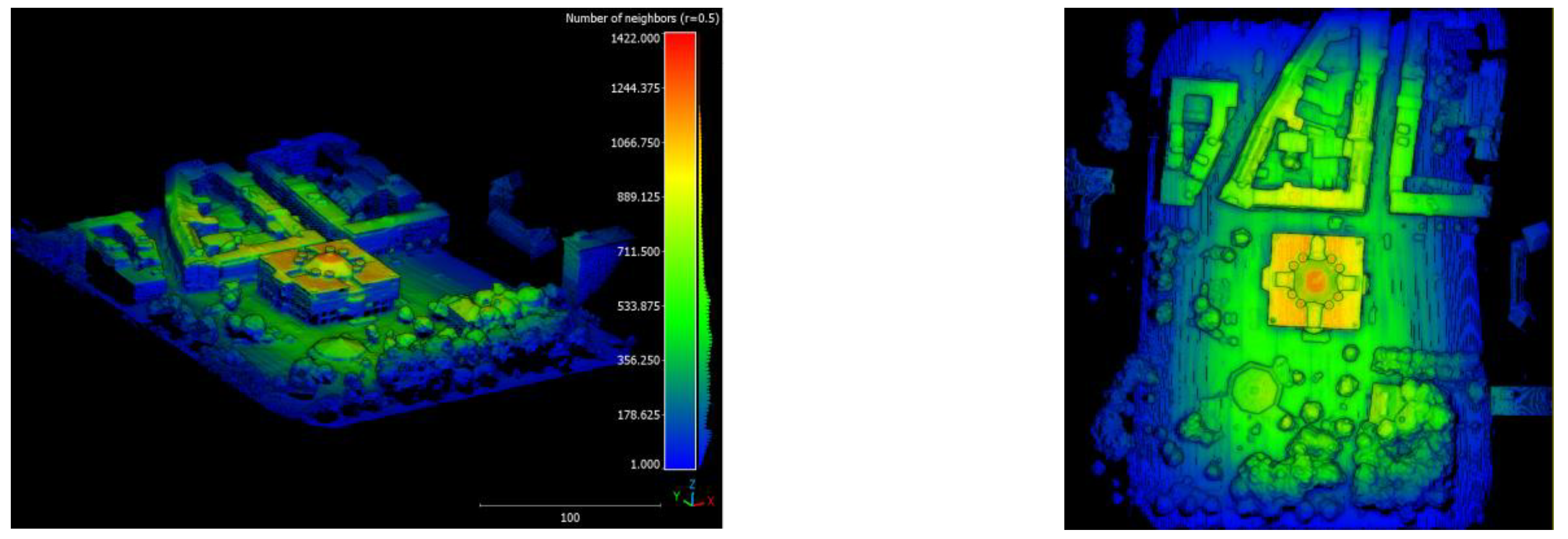
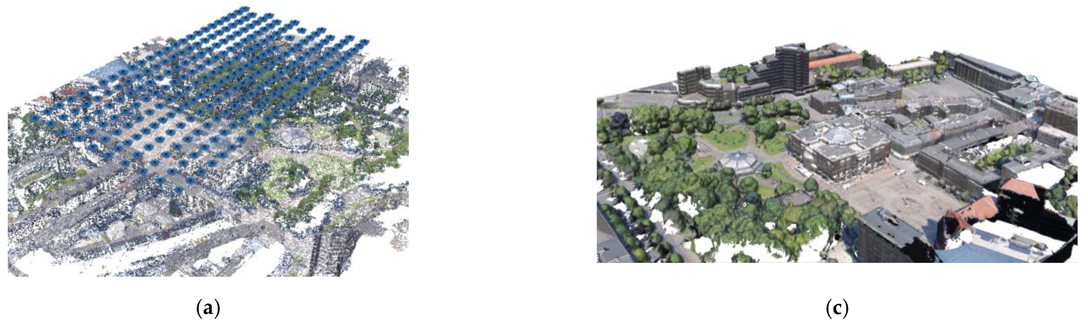
3.2. Use Case #2—Dortmund

The second 3D mapping experiment was simulated over the city of Dortmund (Germany), selecting an area of interest (AOI) of 100 × 200 m² where the flight plans were computed using the developed prototype tool (Section 2.4). The available 3D data are part of the ISPRS/EuroSDR benchmark presented in [51]. In this test, a higher image overlap and a slower flight speed were selected to mimic a more realistic UAV mission planning for 3D modeling tasks. Accordingly, the flight input parameters were selected as follows:

• flying height = 80 m
• speed = 5 m/sec
• end lap = 80% and side lap = 80%

Moreover, for this use case, a set of six ground control points (GCPs) and nine checkpoints (CPs) were distributed over the study area by placing coded targets in the rendered scene.

3.2.1. SenseFly-Based Hybrid UAV Surveying

Given the AOI, the flight input parameters, and the camera specifications, the plan was to capture a total of 665 images along five flight strips. The flight strips, the footprints of the images, and the flight plan are shown in Figure 14. The GSD of the nadir images is 1.8 cm while the oblique views span from 6 to 22 cm.

The processing of the 665 simulated multi-view images successfully recovered the camera poses, with a reprojection error of 0.67 pixels, a multiplicity of ca. 16, and a sparse point cloud of 202,871 points (Figure 15a,b). The root mean square errors (RMSEs) on the GCPs and CPs are shown in

Table 8. Accuracy analyses on the two simulated image datasets over Dortmund and GCP/CP distribution (right).

	RMSE_ XY (mm)	RMSE_Z (mm)	Total RMSE (mm)
	senseFly-based hybrid system
GCPs (6)	2.8 mm	0.5 mm	2.9 mm
CPs (9)	3.7 mm	1.8 mm	4.1 mm
	MAPIR-based hybrid system
GCPs (6)	2.3 mm	2.4 mm	3.3 mm
CPs (9)	4.6 mm	3.3 mm	5.7 mm

. Afterwards, a dense point cloud was created, resulting in ca. 202 million points (Figure 15c,d).

Following the same five flight strips that were planned based on the senseFly multi-view camera, the LiDAR scanning was applied, and a point cloud of ca. 37 million points was produced using the OS1-32 scanner. The density variation of the simulated point cloud is shown in Figure 16, with the red color indicating ≥200 pts/m².

3.2.2. MAPIR-Based Hybrid UAV Surveying

Given the flight input parameters and the camera specifications, a total of ten strips and some 1250 multi-view images were planned and captured. The flight strips, the footprints of the images, and the flight plan are shown in Figure 17. The GSD of the nadir images is 1.5 cm while the oblique views span from 3 to 8 cm.

The bundle block adjustment processing of the rendered MAPIR images over Dortmund closed with a reprojection error of 0.84 pixels, a multiplicity of ca. 13, and a sparse point cloud of 390,801 points (Figure 18a,b). The root mean square errors (RMSEs) on the GCPs and CPs are shown in Table 8. A dense point cloud was created after that with the DIM algorithms, resulting in ca. 159 million points (Figure 18c,d).

Using the same ten flight strips planned for the MAPIR multi-view camera system, the OS1-32 LiDAR scanning was applied and a point cloud of ca. 52 million points was produced (Figure 19).

4. Discussions

The proposed hybrid system for the UAV platforms could clearly be a step forward for the mapping community. The two proposed versions feature different ground coverage due to the different camera specifications. With respect to the aerial hybrid systems, the image’s GSD has a considerable variation between the nadir and the oblique views due to the fixed focal lengths of the chosen cameras. The bundle block adjustments reveal a higher ray multiplicity in the Dortmund dataset due to its higher side lap and slower flying speed. Similarly, the Dortmund dataset has a higher density of the LiDAR points (

Table 9. Summary of the generated and integrated sample point clouds with the proposed hybrid systems for UAV platforms.

	First test		Second test
	senseFly + Ouster	MAPIR + Ouster	senseFly + Ouster	MAPIR + Ouster
Total DIM points	3,165,250	5,516,791	7,523,625	10,818,103
Total LiDAR points	1,100,675	1,692,890	9,593,969	14,289,084
Total Integrated	4,265,925	7,209,681	16,912,628	25,107,187
Density DIM	469 ± 81 pts/m2	804 ± 121 pts/m2	338 ± 77 pts/m2	496 ± 120 pts/m2
Density LiDAR	188 ± 67 pts/m2	296 ± 102 pts/m2	659 ± 340 pts/m2	1050 ± 544 pts/m2
Density Integrated	619 ± 120 pts/m2	1039 ± 178 pts/m2	877 ± 359 pts/m2	1329 ± 575 pts/m2

) with regard to the DIM cloud due to the reduced flying speed (5 m/s). Nevertheless, such issues do not hamper the creation of the dense and accurate point clouds by both of the proposed hybrid systems—as quantitatively shown in the results.

The integration of the camera- and LiDAR-based point clouds visibly show the advantages brought by a hybrid sensor in urban areas (Table 9). As shown in Figure 20, a façade slide was arbitrarily selected on a large building in the Dortmund dataset and the densities of the DIM, LiDAR, and hybrid (integrated) point clouds were computed.

The clear benefit of the proposed hybrid system on the vertical structure is evident. Similarly, the DIM and LiDAR were complementary in some areas where, e.g., the image overlap was not adequate or the LiDAR points did not reach the scene (Figure 21). In both cases, it should be noted that the LiDAR acquisitions were performed based on the flight planning for the images.

Comparing Figure 9 and Figure 12 (as well as Figure 15 and Figure 18), we can notice how the MAPIR-based configuration delivers much denser point clouds due to the larger number of strips. Furthermore, the integration with the photogrammetric point clouds allows the closure of the gaps and also delivers dense results on vertical objects. For illustration, the main building in the scene of the second test was selected to compare the point densities in the three collected point clouds of the LiDAR and DIM and when they are integrated together using both suggested hybrid sensors (Figure 22).

5. Conclusions

The paper proposed a novel hybrid system for the UAV platform. The proposed data acquisition system is composed of five RGB cameras and a LiDAR sensor. Using a dedicated flight planning tool (shared with the community at https://github.com/Photogrammtery-Topics/flight-planning-tool-for-Hybrid-UAV-system-accessed on 18 October 2022), the flying strips, multi-view image acquisition, and LiDAR scanning can be planned and simulated. The acquired and processed data revealed that the proposed hybrid system is highly suitable for 3D mapping purposes in urban scenarios. The integrated point clouds also show very high density in cluttered and vertical areas, with ground accuracies acceptable for mapping and cartographic purposes. The system could make 3D modeling easier and more automated, reducing processing time and paving the road for the fast and automated upgrading of the existing city models.

So far, the integration of the image- and range-based point clouds is a pure merging, but smart data fusion could be applied in order to refine the final 3D surveying product.

The proposed hybrid sensors could also include a multispectral camera (instead of the RGB nadir view) in order to couple the geometric data with the spectral information, which is useful, e.g., for vegetation mapping, 3D NDVI map production, etc. With respect to LiDAR, the OS1-32 digital scanner was suggested; however, the proposed hybrid system can be adapted to place different LiDAR types, such as Livox, Quanergy M8, Velodyne Puck, etc.

References

1. Colomina, I.; Molina, P. Unmanned Aerial Systems for Photogrammetry and Remote Sensing: A Review. ISPRS J. Photogramm. Remote Sens. 2014, 92, 79–97. [Google Scholar] [CrossRef] [Green Version]
2. Nex, F.; Remondino, F. Uav for 3d Mapping Applications: A Review. Appl. Geomat. 2014, 6, 1–15. [Google Scholar] [CrossRef]
3. Hassanalian, M.; Abdelkefi, A. Classifications, Applications, and Design Challenges of Drones: A Review. Prog. Aerosp. Sci. 2017, 91, 99–131. [Google Scholar] [CrossRef]
4. Granshaw, S.I. Rpv, Uav, Uas, Rpas … or Just Drone? Photogramm. Rec. 2018, 33, 160–170. [Google Scholar] [CrossRef]
5. Yao, H.; Qin, R.; Chen, X. Unmanned Aerial Vehicle for Remote Sensing Applications—A Review. Remote Sens. 2019, 11, 1443. [Google Scholar] [CrossRef] [Green Version]
6. Francesco, I.; Bianchi, A.; Cina, A.; Michele, C.D.; Maschio, P.; Passoni, D.; Pinto, L. Mid-Term Monitoring of Glacier’s Variations with UAVs: The Example of the Belvedere Glacier. Remote Sens. 2022, 14, 28. [Google Scholar]
7. Nex, F.; Armenakis, C.; Cramer, M.; Cucci, D.A.; Gerke, M.; Honkavaara, E.; Kukko, A.; Persello, C.; Skaloud, J. Uav in the Advent of the Twenties: Where We Stand and What Is Next. ISPRS J. Photogramm. Remote Sens. 2022, 184, 215–242. [Google Scholar] [CrossRef]
8. Steenbeek, A.; Nex, F. Cnn-Based Dense Monocular Visual Slam for Real-Time Uav Exploration in Emergency Conditions. Drones 2022, 6, 79. [Google Scholar] [CrossRef]
9. Giordan, D.; Hayakawa, Y.; Nex, F.; Remondino, F.; Tarolli, P. Review Article: The Use of Remotely Piloted Aircraft Systems (Rpass) for Natural Hazards Monitoring and Management. Nat. Hazards Earth Syst. Sci. 2018, 18, 1079–1096. [Google Scholar] [CrossRef] [Green Version]
10. Wang, D.; Xing, S.; He, Y.; Yu, J.; Xu, Q.; Li, P. Evaluation of a New Lightweight Uav-Borne Topo-Bathymetric Lidar for Shallow Water Bathymetry and Object Detection. Sensors 2022, 22, 1379. [Google Scholar] [CrossRef]
11. Agrafiotis, P.; Skarlatos, D.; Georgopoulos, A.; Karantzalos, K. Shallow Water Bathymetry Mapping from Uav Imagery Based on Machine Learning. Int. Arch. Photogramm. Remote Sens. Spatial Inf. Sci. 2019, XLII-2/W10, 9–16. [Google Scholar] [CrossRef]
12. Rossi, M.; Brunelli, D.; Adami, A.; Lorenzelli, L.; Menna, F.; Remondino, F. Gas-Drone: Portable gas sensing system on UAVs for gas leakage localization. In Proceedings of the SENSORS, 2014 IEEE, Valencia, Spain, 2–5 November 2014; pp. 1431–1434. [Google Scholar]
13. Rohi, G.; Ejofodomi, O.; Ofualagba, G. Autonomous Monitoring, Analysis, and Countering of Air Pollution Using Environmental Drones. Heliyon 2020, 6, e03252. [Google Scholar] [CrossRef] [PubMed] [Green Version]
14. Skondras, A.; Karachaliou, E.; Tavantzis, I.; Tokas, N.; Valari, E.; Skalidi, I.; Bouvet, G.A.; Stylianidis, E. Uav Mapping and 3d Modeling as a Tool for Promotion and Management of the Urban Space. Drones 2022, 6, 115. [Google Scholar] [CrossRef]
15. Stöcker, C.; Koeva, M.N.; Zevenbergen, J.A. Uav Technology: Opportunities to Support the Updating Process of the Rwandan Cadastre. In Proceedings of the 10th East Africa Land Administration Network (EALAN) Conference 2019, Ruhengeri, Rawanda, 21–25 July 2019. [Google Scholar]
16. Koeva, M.; Stöcker, C.; Crommelinck, S.; Ho, S.; Chipofya, M.; Sahib, J.; Bennett, R.; Zevenbergen, J.; Vosselman, G.; Lemmen, C.; et al. Innovative Remote Sensing Methodologies for Kenyan Land Tenure Mapping. Remote Sens. 2020, 12, 273. [Google Scholar] [CrossRef] [Green Version]
17. Immerzeel, W.W.; Kraaijenbrink, P.D.A.; Shea, J.M.; Shrestha, A.B.; Pellicciotti, F.; Bierkens, M.F.P.; De Jong, S.M. High-Resolution Monitoring of Himalayan Glacier Dynamics Using Unmanned Aerial Vehicles. Remote Sens. Environ. 2014, 150, 93–103. [Google Scholar] [CrossRef]
18. Ren, H.; Zhao, Y.; Xiao, W.; Hu, Z. A Review of Uav Monitoring in Mining Areas: Current Status and Future Perspectives. Int. J. Coal Sci. Technol. 2019, 6, 320–333. [Google Scholar] [CrossRef] [Green Version]
19. Li, X.; Li, Z.; Wang, H.; Li, W. Unmanned Aerial Vehicle for Transmission Line Inspection: Status, Standardization, and Perspectives. Front. Energy Res. 2021, 9, 713634. [Google Scholar] [CrossRef]
20. Mandirola, M.; Casarotti, C.; Peloso, S.; Lanese, I.; Brunesi, E.; Senaldi, I. Use of Uas for Damage Inspection and Assessment of Bridge Infrastructures. Int. J. Disaster Risk Reduct. 2022, 72, 102824. [Google Scholar] [CrossRef]
21. Kern, A.; Fanta-Jende, P.; Glira, P.; Bruckmüller, F.; Sulzbachner, C. An Accurate Real-Time Uav Mapping Solution for the Generation of Orthomosaics and Surface Models. Int. Arch. Photogramm. Remote Sens. Spatial Inf. Sci. 2021, XLIII-B1-2, 165–171. [Google Scholar] [CrossRef]
22. Elmokadem, T.; Savkin, A.V. Towards Fully Autonomous Uavs: A Survey. Sensors 2021, 21, 6223. [Google Scholar] [CrossRef]
23. Toschi, I.; Remondino, F.; Rothe, R.; Klimek, K. Combining Airborne Oblique Camera and Lidar Sensors: Investigation and New Perspectives. Int. Arch. Photogramm. Remote Sens. Spatial Inf. Sci. 2018, XLII-1, 437–444. [Google Scholar] [CrossRef]
24. Toschi, I.; Farella, E.; Welponer, M.; Remondino, F. Quality-Based Registration Refinement of Airborne Lidar and Photogrammetric Point Clouds. ISPRS J. Photogramm. Remote Sens. 2021, 172, 160–170. [Google Scholar] [CrossRef]
25. Toschi, I.; Remondino, F.; Hauck, T.; Wenzel, K. When photogrammetry meets LiDAR: Towards the airborne hybrid era. GIM Int. 2019, 17–21. [Google Scholar]
26. Shan, J.; Toth, C.K. Topographic Laser Ranging and Scanning: Principles and Processing, 1st ed.; CRC Press: Boca Raton, FL, USA, 2009. [Google Scholar]
27. Vosselman, G.; Maas, H.-G. Airborne and Terrestrial Laser Scanning; Whittles Publishing: Scotland, UK, 2010. [Google Scholar]
28. Haala, N.; Rothermel, M. Dense Multiple Stereo Matching of Highly Overlapping Uav Imagery. Int. Arch. Photogramm. Remote Sens. Spatial Inf. Sci. 2012, XXXIX-B1, 387–392. [Google Scholar] [CrossRef] [Green Version]
29. Remondino, F.; Spera, M.G.; Nocerino, E.; Menna, F.; Nex, F.C. State of the Art in High Density Image Matching. Photogramm. Rec. 2014, 29, 144–166. [Google Scholar] [CrossRef] [Green Version]
30. Rupnik, E.; Nex, F.C.; Toschi, I.; Remondino, F. Aerial Multi—Camera Systems: Accuracy and Block Triangulation Issues. ISPRS J. Photogramm. Remote Sens. 2015, 101, 233–246. [Google Scholar] [CrossRef]
31. Remondino, F.; Gerke, M. Oblique Aerial Imagery: A Review. In Proceedings of the Photogrammetric Week ’15, Stuttgart, Germany, 7–11 September 2015; Frietsch, D., Ed.; Wichmann: Stuttgart, Germany, 2015; pp. 75–83. [Google Scholar]
32. Moe, K.; Toschi, I.; Poli, D.; Lago, F.; Schreiner, C.; Legat, K.; Remondino, F. Changing the Production Pipeline—Use of Oblique Aerial Cameras for Mapping Purposes. Int. Arch. Photogramm. Remote Sens. Spatial Inf. Sci. 2016, XLI-B4, 631–637. [Google Scholar]
33. Toschi, I.; Ramos, M.M.; Nocerino, E.; Menna, F.; Remondino, F.; Moe, K.; Poli, D.; Legat, K.; Fassi, F. Oblique Photogrammetry Supporting 3d Urban Reconstruction of Complex Scenarios. Int. Arch. Photogramm. Remote Sens. Spatial Inf. Sci. 2017, XLII-1/W1, 519–526. [Google Scholar] [CrossRef] [Green Version]
34. Remondino, F.; Toschi, I.; Gerke, M.; Nex, F.; Holland, D.; McGill, A.; Talaya Lopez, J.; Magarinos, A. Oblique Aerial Imagery for Nma—Some Best Practices. Int. Arch. Photogramm. Remote Sens. Spatial Inf. Sci. 2016, XLI-B4, 639–645. [Google Scholar] [CrossRef] [Green Version]
35. Bláha, M.; Eisenbeiss, H.; Grimm, D.; Limpach, P. Direct Georeferencing of Uavs. Int. Arch. Photogramm. Remote Sens. Spatial Inf. Sci. 2012, XXXVIII-1, 131–136. [Google Scholar] [CrossRef] [Green Version]
36. Masiero, A.; Fissore, F.; Vettore, A. A Low Cost Uwb Based Solution for Direct Georeferencing Uav Photogrammetry. Remote Sens. 2017, 9, 414. [Google Scholar] [CrossRef] [Green Version]
37. Liu, X.; Lian, X.; Yang, W.; Wang, F.; Han, Y.; Zhang, Y. Accuracy Assessment of a Uav Direct Georeferencing Method and Impact of the Configuration of Ground Control Points. Drones 2022, 6, 30. [Google Scholar] [CrossRef]
38. Grayson, B.; Penna, N.T.; Mills, J.P.; Grant, D.S. Gps Precise Point Positioning for Uav Photogrammetry. Photogramm. Rec. 2018, 33, 427–447. [Google Scholar] [CrossRef]
39. Valente, D.S.M.; Momin, A.; Grift, T.; Hansen, A. Accuracy and Precision Evaluation of Two Low-Cost Rtk Global Navigation Satellite Systems. Comput. Electron. Agric. 2020, 168, 105142. [Google Scholar] [CrossRef]
40. Famiglietti, N.; Cecere, G.; Grasso, C.; Memmolo, A.; Vicari, A. A Test on the Potential of a Low Cost Unmanned Aerial Vehicle Rtk/Ppk Solution for Precision Positioning. Sensors 2021, 21, 3882. [Google Scholar] [CrossRef]
41. MAPIR. Survey3: Multi-Spectral Survey Cameras. Available online: https://www.mapir.camera/pages/survey3-cameras (accessed on 18 October 2022).
42. Sensefly. Sensefly, S.O.D.A. Available online: https://www.sensefly.com/camera/sensefly-soda-photogrammetry-camera/ (accessed on 18 October 2022).
43. Bashar, A.; Remondino, F. Flight Planning for Lidar-Based Uas Mapping Applications. ISPRS Int. J. Geo-Inf. 2020, 9, 378. [Google Scholar]
44. Ouster. Digital Vs Analog Lidar. Available online: https://www.youtube.com/watch?v=yDPotPQfRTE&feature=emb_logo (accessed on 1 October 2022).
45. Höhle, J. Oblique Aerial Images and Their Use in Cultural Heritage Documentation. Int. Arch. Photogramm. Remote Sens. Spatial Inf. Sci. 2013, XL-5/W2, 349–354. [Google Scholar] [CrossRef] [Green Version]
46. Wolf, P.; De Witt, B. Elements of Photogrammetry with Applications in Gis, 3rd ed.; McGraw Hill: NewYork, NY, USA, 2000. [Google Scholar]
47. Alsadik, B. Adjustment Models in 3d Geomatics and Computational Geophysics: With Matlab Examples; Elsevier: Amsterdam, The Netherlands, 2019. [Google Scholar]
48. Bllender. Available online: http://www.blender.org (accessed on 18 October 2022).
49. Agisoft. Agisoft Metashape. Available online: http://www.agisoft.com/downloads/installer/ (accessed on 18 October 2022).
50. Launceston City 3d Model. Available online: http://s3-ap-southeast-2.amazonaws.com/launceston/atlas/index.html (accessed on 18 October 2022).
51. Nex, F.; Gerke, M.; Remondino, F.; Przybilla, H.-J.; Bäumker, M.; Zurhorst, A. Isprs Benchmark for Multi-Platform Photogrammetry. ISPRS Ann. Photogramm. Remote Sens. Spatial Inf. Sci. 2015, II-3/W4, 135–142. [Google Scholar] [CrossRef]
Figure 1. Example of commercially available multi-view cameras for UAV platform (Table 1): Viewprouav (a), Shareuavtex (b), DroneBase (c), ADTi (d), Quantum-System (e), and JOUAV (f).
Drones 06 00314 g001
Figure 2. The chosen MAPIR Survey 3 (a), senseFly SODA (b), and Ouster OS1-32 (c).
Drones 06 00314 g002
Figure 3. Hybrid MAPIR + Ouster system showing its internal arrangement, dimensions, and footprint patterns on the ground (a); hybrid senseFly + Ouster system showing its internal arrangement, dimensions, and footprint patterns on the ground (b).
Drones 06 00314 g003
Figure 4. The GUI of the developed flight planning tool for hybrid UAV-based sensors (a). The image footprints plot for a given flight and sensor configuration (b).
Drones 06 00314 g004
Figure 5. UAV flight planning design parameters illustration for both sensors used.
Drones 06 00314 g005
Figure 6. Methodology workflow.
Drones 06 00314 g006
Figure 7. Examples of the GCPs/CPs used in the photogrammetric adjustments of the simulated datasets.
Drones 06 00314 g007
Figure 8. Flight planning with the senseFly camera over Launceston: five strips and 475 multi-view images.
Drones 06 00314 g008
Figure 9. Recovered camera poses and sparse point cloud for the simulated senseFly-based multi-view image block (475 images) over Launceston (a,b). Derived dense point cloud (c,d).
Drones 06 00314 g009
Figure 10. Density (radius = 50 cm) of the LiDAR-based point cloud created by the Ouster LiDAR using the senseFly-based hybrid system over Launceston.
Drones 06 00314 g010
Figure 11. Flight planning with the MAPIR camera over Launceston: seven strips and 910 images.
Drones 06 00314 g011
Figure 12. Recovered camera poses and sparse point cloud for the simulated MAPIR-based multi-view image block (910 images) over Launceston (a,b). Derived dense point cloud (c,d).
Drones 06 00314 g012
Figure 13. Density (radius = 50 cm) of the LiDAR-based point cloud created by the Ouster scanner using the MAPIR-based hybrid system over Launceston.
Drones 06 00314 g013
Figure 14. Flight planning with the senseFly camera over Dortmund: five strips and 665 images.
Drones 06 00314 g014
Figure 15. Recovered camera poses and sparse point cloud for the simulated senseFly-based multi-view image block (665 images) over Dortmund (a,b). Derived DIM point cloud (c,d).
Drones 06 00314 g015
Figure 16. Density (radius = 50 cm) of the LiDAR-based point cloud created by the Ouster scanner using the senseFly-based hybrid system over Dortmund.
Drones 06 00314 g016
Figure 17. Flight planning with the MAPIR camera over Dortmund: ten strips and 1250 overlapping multi-view images.
Drones 06 00314 g017
Figure 18. Recovered camera poses and sparse point cloud for the simulated MAPIR-based multi-view image block (1250 images) over Dortmund (a,b). Derived dense point cloud (c,d).
Drones 06 00314 g018aDrones 06 00314 g018b
Figure 19. Density (radius = 50 cm) of the LiDAR-based point cloud created by the Ouster LiDAR using the MAPIR-based hybrid system over Dortmund.
Drones 06 00314 g019
Figure 20. Plots of density profiles on a building façade in Dortmund.
Drones 06 00314 g020
Figure 21. Photogrammetric point cloud (left) and LiDAR point cloud (right) with highlighted areas of complementarity between the two datasets.
Drones 06 00314 g021
Figure 22. A comparison of the point density and improvement after integrating point clouds from LiDAR and DIM. For both hybrid sensors, the point clouds shown have the same minimum and maximum limits.
Drones 06 00314 g022