Automatic Tuning and Turbulence Mitigation for Fixed-Wing UAV with Segmented Control Surfaces

Abstract

Unlike bigger aircraft, the small fixed-wing unmanned aerial vehicles face significant stability challenges in a turbulent environment. To improve the flight performance, a fixed-wing UAV with segmented aileron control surfaces has been designed and deployed. A total of four ailerons are attached to the main wing and grouped into inner and outer aileron pairs. The controllers are automatically tuned by utilizing the frequency response data obtained via the frequency sampling filter and the relay with embedded integrator experiments. The hardware validation experiments are performed in the normal and turbulent flight environments under three configurations: inner aileron pair only, outer aileron pair only and collective actuation of all the aileron pairs. The error-threshold-based control is introduced to handle collective actuation of aileron pairs. The experiments have manifested that the collective usage of all aileron segments improves the roll attitude stability by a margin of $38.69\%$ to $43.51\%$ when compared to the independent actuation of aileron pairs in a turbulent atmosphere.

1. Introduction

Small unmanned aerial vehicles (UAVs) are very well known for their long-flight endurance. This capability of the fixed-wing aircraft is further extended through various techniques which use the structure of the aircraft to extract energy from the surrounding wind, and achieve even longer flights [1,2]. Unlike the multirotor UAV, the fixed-wing aircraft enjoy the luxury of a bigger surface area. The latest work reports the deployment of light weight solar panels on to the most of the available surface area of the fixed-wing UAV to generate power and enhance its flight time [3]. Fixed-wing UAVs are also used to quickly and securely deliver life-saving medicines and products to the distant and hilly areas [4,5]. Some other mature applications include the terrain mapping [6,7], collection of data using obstacle avoidance techniques [8,9], forestry and coastal surveys [10,11] and telecommunication [12,13,14].

The small fixed-wing UAVs are usually more susceptible to wind gusts. The sensitivity to wind gusts or the random pressure changes in the environment is mainly associated with the size of the main wing, specifically when its size is smaller than the wind disturbance envelope [15]. Consequently, a harsh flight environment has an adverse impact on all of the axes governing the stability of the airplane, especially the roll axis [16]. The poor roll control leads to significant flight deviations along with altitude fluctuations. In the case of small and high-frequency disturbances, the actuators’ working bandwidth limitation is also the main cause of the degraded performance of aircraft even if it is using the novel turbulence sensing techniques [17,18]. As far as the structure of a fixed-wing UAV is concerned, the literature reports many attempts to enhance the performance of the fixed-wing UAV. Examples include the airplane with segmented control surfaces [19,20,21], flexible-wing design [22,23,24,25,26] blended wing body design [27] and split-aileron wing [28]. By the design itself, the segmented aileron control surfaces are explored in [19,20], demonstrating their practicality and advantages. The segmented surfaces have couple of aerodynamic advantages as well such as improvement in active wing lift distribution profile and reduction in drag force by working in favor of rudder and pitch control surfaces [19]. The segmented ailerons have also been used in in-flight load distribution by incorporating optical fibers as wing strain sensors [29]. Various segments are selectively actuated to recover from wing fluttering which is linked with poor flight performance. Modern commercial aircraft also utilize the segmented ailerons to mitigate the wing fluttering, which leads to more comfortable and safe air travel [30]. For instance, multiple ailerons are integrated in the Airbus 380 and are engaged in different ways depending on the speed of the aircraft [31]. Although the physical designs for the small fixed-wing aircraft with many aileron segments may exist in the literature, a thorough system identification study and a control architecture has not yet been developed and analyzed for such an aircraft. However, for ordinary small fixed-wing UAV with single aileron pair, i.e., one aileron control surface on each side of the main wing, several advances and optimization are reported in the literature. Notable work includes the use of PID controller [32,33,34], sliding mode controller [35,36], model predictive controller (MPC) [37,38], fuzzy controller [39] and back-stepping based control in [40,41].

PID controllers continue to be the most widely used because of their straightforward structure and practical ease of implementation [42]. Additionally, they do not require a lot of computational resources. The ability to modify controller parameters without comprehension of a plant’s model is one of the benefits of PID controllers. Online experimental testing is another way to fine-tune the PID controller parameters for unmanned aerial vehicles [43]. These attributes have led to the adoption of PID controllers in the multitude of commercially available autopilot flight controllers today, such the Acro Naze32, Mikrokopter, Ardupilot, Paparazzi auto-pilot and Micropilot, etc. Furthermore, PID controllers’ instant parameter adjustment and seamless implementation make them ideally suited for cascade control architecture. For the dynamically complicated systems, an optimum control strategy is attained using a cascaded PID control architecture [44]. In other words, larger and complicated system can be divided into smaller, independent subsystems, and then PID controllers are asynchronously tuned exclusively based on the dynamics of each deconstructed subsystem [45,46]. One of the most significant challenges when developing the controller for a UAV is tuning the controller parameters. The UAV control system’s cascade control structure makes the tuning process even more arduous, especially when the UAV’s nonlinear mathematical model is incorporated.

This study presents the detailed process of the system identification and the roll attitude control design of the fixed-wing UAV with multiple aileron control surfaces. For the experimental purposes, the main and severely disturbed axis in the turbulence, i.e., the roll axis, is taken into consideration. For a cascade control system of a fixed-wing UAV with multiple segmented ailerons, an automatic tuning method is suggested. In a supervised experimental environment, closed-loop experiments are conducted in order to automatically acquire a time-invariant model of the aircraft’s roll dynamics. Following that, PID controllers are designed for the cascade control system using the frequency points. The aircraft undergoes the relay feedback experiment to proceed with the autotuning methodology. To recursively approximate the closed-loop fundamental frequency, responses from relay feedback tests are used [47]. Additionally, the PID controllers are tuned using the tuning guidelines suggested in [48] when the appropriate frequency points on the Nyquist plot are determined for the given aircraft. Finally, a cascade PID control system is enacted and validated using experimental results. Following is a summary of this paper’s novel contributions:

1.

A robust roll attitude control system of the fixed-wing UAV with multiple aileron segments is designed utilizing autotuning methodology. At first, this UAV is subjected to the process of system identification via relay instrument to acquire frequency response points. The process of system identification from scratch is thorough as it captures not only the complex system’s actual dynamics, but also those which might impact the closed-loop operation of control system such as computation delays, sensors, and actuators. Afterward, the acquired frequency points are directly used to design and autotune the PID controllers based on simplistic sensitivity functions and beta values as discussed later on. The suggested autotuning methodology is straightforward and does not require any prior information on the plant;

2.

In order to efficiently deal with the complexity of the system, the proposed control system is designed to have cascade. As discussed later on, unique controllers are handling the actuation of the inner and outer aileron segments through a cascade control system by considering each aileron pair as an independently manipulated variable. Moreover, a novel error-threshold control technique is proposed and incorporated to firmly reject the severe turbulence and other external disturbances. The experimental results have shown that such method of the controller tuning and multiple aileron control leads to highly stable and pleasant flight.

3.

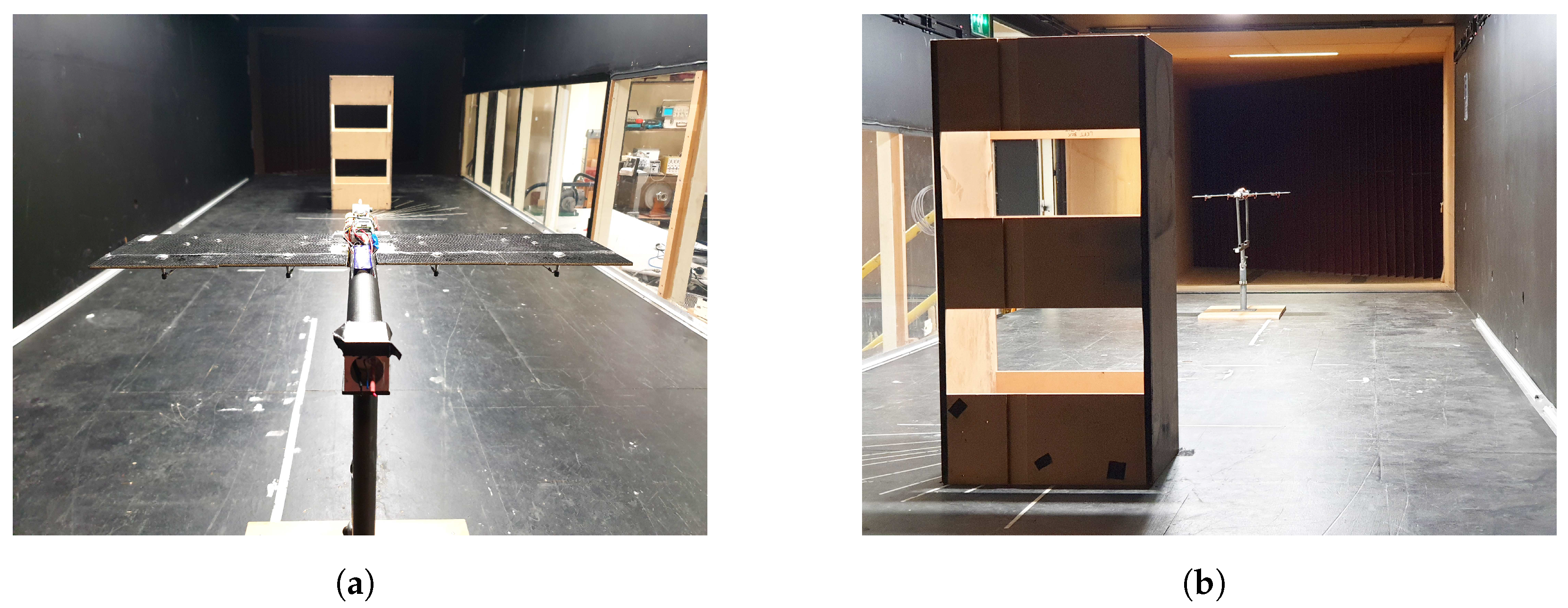
A complete hardware of the fixed-wing UAV with multiple aileron segments along with a custom flight control board is designed to test and validate the efficacy of the autotuing methodology and multi-segment design against turbulence mitigation. All the experiments documented in this work we performed in a professional wind tunnel environment situated in RMIT University. The acquired results demonstrate that the fixed-wing UAV with multiple aileron segments can easily perform in-flight switching between a conventional and multi-segmented UAV, whereas asserting that the multi-segment configuration exhibits stronger disturbance rejection characteristics during a hostile flight environment.

The paper is structured as follows. Section 2 details the hardware specifications of the multi-segment fixed-wing UAV along with the environment in which the experiments have been conducted. The conventional non-linear mathematical model of a common fixed-wing UAV is also explained. Section 3 describes the relay experiment which is utilized to discover unknown dynamics of the system. This section also explains the step by step process of frequency response extraction and controller design. Section 4 provides the numerical explanation of inner and outer loop controllers design for cascade system by utilizing two frequency points. Section 5 presents the cascade control structure implementation for the roll axis and the related hardware validation experiments. Section 6 provides the novel technique to control all the segments based on the roll angle deviation to enhance the stability of the aircraft. Section 7 summarizes the research findings and future directions.

2. Aircraft Structure and Mathematical Model

The hardware specifications and the experimental environment of the fixed-wing UAV with multiple aileron control surfaces are described in this section.

2.1. Specifications of the Aircraft with Multiple Control Surfaces

Unlike the conventional fixed-wing UAV, each aileron control surface is segmented into two to achieve the multi-segment configuration. In this way, each side of the main wing gets two ailerons, resulting into a total of four aileron control surfaces for the aircraft under consideration. Figure 1 presents the detailed illustration of the experimental UAV with four aileron control surfaces. It depicts the measurements of the main wing size, dimensions of the ailerons, and arrangement of the multiple aileron segments. It should be noted that orientation of the ailerons as shown in Figure 1 is only for understanding the concept of multiple ailerons’ arrangement. Such an orientation will result in aerial braking and is not deployed in any of experiments presented later in this work. Figure 2 illustrates the aircraft’s segmented control surfaces, i.e., the inner and outer aileron pairs. The description of the important parameters of the UAV are presented by

Table 1. Features of UAV.

Features	Details
Airfoil	Flat plate
Wing length	290.0 mm
Chord	160 mm
Cruise speed	10.0 m
Camber	4.0 mm
Aileron segment size	145 × 45 mm

.

2.2. Control Hardware

The aircraft’s flight control board utilizes Cortex M4 processor (32-bit) to process attitude data and control algorithms. It runs at the clock speed of 180 Mhz which ensures high speed control code execution with minimum latency. The roll rate and angle of the UAV is precisely estimated through the well-known MPU6050 chip. This attitude sensing device has the capability to process the data from all axes, i.e., from gyro and accelerometer via onboard DMP (digital motion processor) [49] to accurately provide the orientation of a body in 3D space. Another benefit of onboard DMP is that the main processor is relieved of any additional load of filtering the noisy aircraft attitude data. Thus, the main processor is completely dedicated to execute control algorithms with minimum delay which is essential for real-time control applications.

The description of hardware components used to develop flight control system is presented in

Table 2. Parts used in UAV.

Components	Details
Micro-controller	MK64FX512VMD12
Attitude sensor	MPU6050 with DMP
Servo	KST10
Data Logger	OpenLog (blackbox)
Voltage Regulator	Step-down DC–DC converter

. A set of highly agile servos namely KST10 is deployed to minimize the effects of the actuator delay into the control loop. Moreover, the servos are top of their class and incorporate metallic gears to ensure consistent behavior and sustain the additional stress induced due to their high speed performance. The properties of these servos are given by

Table 3. High-speed servo features.

Specifications	Details
Operating Voltage	4.8–7.4 V
Speed	0.04 s/60${}^{\circ }$ @ 7.4 V
Input pulse	800 $\mathsf{\mu }$S to 2200 $\mathsf{\mu }$S
Torque	3.4 kg/cm @ 7.4 V
Gear Type	All Metal Gear
Weight	20 g

. Furthermore, instead of relying on off-the-shelf commercial flight controllers, a customized flight control board (FCB) is designed for the aircraft under consideration. The FCB is designed to fit around a Teensy 3.5 microcontroller board in the software environment of Altium 17. The final version of the assembled FCB is presented in Figure 3.

2.3. Experimental Setup

The wind tunnel facility used in the experiments is known as RMIT Industrial Wind Tunnel (IWT). This wind tunnel has a hexagonal test section measuring $3\times 2\times 9$ meters (W × H × L). A 225 kilowatt DC motor, capable of producing a maximum of 50 m/s airspeed, precisely controls the airspeed inside the tunnel. The test section is fitted with a pilot static tube to measure airspeed. This type of tube works by measuring differential air pressure using two holes. The front hole directly interacts with the moving airstream to measure stagnation pressure relative to static pressure, which is read by the side hole. The differential air pressure is then converted to the appropriate airspeed using standard mathematical relations. Additional details pertinent to the characteristics of the IWT are discussed in [50]. The IWT is also equipped with anechoic turning vanes, which reduce the acoustic noise to a significantly low amplitude in the test section [51,52]. It is common practice to test the aerodynamic properties and flight in an indoor wind tunnel environment due to the controllability and repeatability of particular wind speed and customizable turbulence spectrum. As the model selected for this work is novel, i.e., with multiple control surfaces, a repeatable flight environment is essential in order to allow for various performances and establish the effectiveness of multi-segment control design in normal and hostile flight conditions.

2.4. Mathematical Model for Conventional Fixed-Wing Aircraft

In order to understand the novelty and supremacy of the proposed control system design in upcoming sections, it is important to become familiar with the basic dynamical model of a conventional fixed-wing airplane. The differential equations defining roll (p), pitch (q) and yaw (r) in the body frame of a conventional fixed-wing UAV are described by (1) [53,54]. The control variables are the ailerons, elevator and rudder deflections, defined as variables ${\delta }_a$, ${\delta }_e$ and ${\delta }_r$, respectively. Among the remaining parameters, $C_{x_y}$ is the aerodynamics derivative coefficients corresponding to their respective variables, ${\mathsf{\Gamma }}_x$ defines coupling dynamics, $\rho$ is the air density, $V_a$ is the airspeed, S is the wing platform area, b is the wingspan of the airframe, c is the mean chord of the wing, and ${\beta }_C$ is the course angle.

$$\begin{array}{cc}\hfill \dot{p}& ={\mathsf{\Gamma }}_{1}pq-{\mathsf{\Gamma }}_{2}qr+\frac{1}{2}\rho V_a^{2}Sb\left[C_{{\ell }_0}+C_{{\ell }_{{\beta }_C}}{\beta }_C+C_{{\ell }_p}\frac{bp}{2V_a}+C_{{\ell }_r}\frac{br}{2V_a}+C_{{\ell }_{{\delta }_a}}{\delta }_a+C_{{\ell }_{{\delta }_r}}{\delta }_r\right]\hfill \\ \hfill \dot{q}& ={\mathsf{\Gamma }}_{5}pr-{\mathsf{\Gamma }}_6(p^2-r^2)+\frac{\rho V_a^{2}Sc}{2I_y}\left[C_{m_0}+C_{m_{\alpha }}+C_{m_q}\frac{cq}{2V_a}+C_{m_{{\delta }_e}}{\delta }_e\right]\hfill \\ \hfill \dot{r}& ={\mathsf{\Gamma }}_{7}pq-{\mathsf{\Gamma }}_{1}qr+\frac{1}{2}\rho V_a^{2}Sb\left[C_{n_0}+C_{n_{{\beta }_C}}{\beta }_C+C_{n_p}\frac{bp}{2V_a}+C_{n_r}\frac{br}{2V_a}+C_{n_{{\delta }_a}}{\delta }_a+C_{n_{{\delta }_r}}{\delta }_r\right]\hfill \end{array}$$

(1)

In the complete attitude control system of a UAV, there are three major parameters which are precisely monitored, namely, roll, pitch Euler angles, and yaw angular velocity, denoted by $\varphi ,\theta$ and r, respectively. A standard set of matrices that connects body frame angular rates with the Euler angular rates is represented through equations given by (2).

$$\left[\begin{array}{c}\dot{\varphi }\\ \dot{\theta }\\ \dot{\psi }\end{array}\right]=\left[\begin{array}{ccc}1& sin\left(\varphi \right)tan\left(\theta \right)& cos\left(\varphi \right)tan\left(\theta \right)\\ 0& cos\left(\varphi \right)& -sin\left(\varphi \right)\\ 0& sin\left(\varphi \right)sec\left(\theta \right)& cos\left(\varphi \right)sec\left(\theta \right)\end{array}\right]\left[\begin{array}{c}p\\ q\\ r\end{array}\right]$$

(2)

Let suppose the reference commands from a pilot operating a UAV are denoted by (${\varphi }^{*},{\theta }^{*}$ and $r^{*}$). The ideal control objective is to make the UAV’s roll, pitch angles and yaw rate track the designated reference-points with zero error, thereby rejecting any externally inflicted disturbance such as wind gusts or payload fluctuations. It is necessary to discuss the mathematical model presented by (1) and (2) for a conventional fixed-wing aircraft. Although the given model is precise, building a model-based control system will require a knowledge of many unknown parameters. Clearly, finding these unknown parameters is a highly time-consuming and cumbersome job. The control system design problem is tackled more effectively by the direct identification of linear model and automatic tuning of controllers while residing within the actual flight environment (i.e., the wind tunnel) as described in following sections.

3. System Dynamics and Controller Design Using Two Frequency Points

This section describes the benefits of conducting a relay with integrator experiments, as well as use of the frequency sampling filter (FSF) methodology to acquire the frequency response points along with the controller design technique.

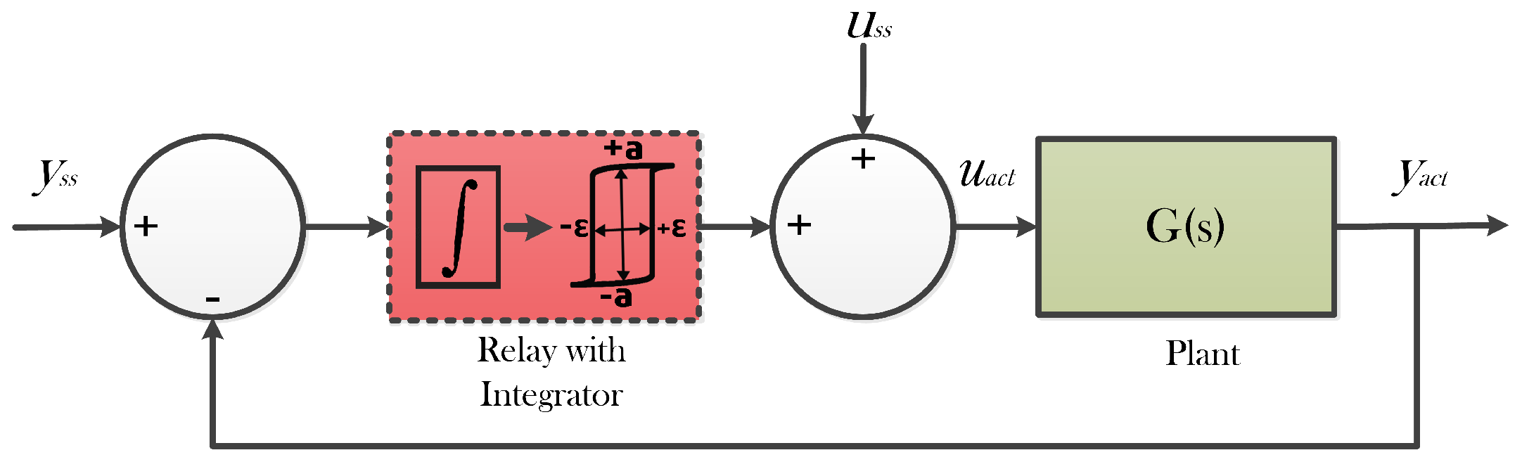
3.1. Relay with Integrator-Based System Identification

A relay with an embedded integrator mainly assists in identifying the location of fundamental frequency ${\omega }_1$ of an unknown plant. Such an experiment produces ${\omega }_1$ that passes through the imaginary axis of the Nyquist plot [48]. The relay with integrator experiment generates ${\omega }_1$ with lower frequency when compared with the one using relay with hysteresis. Figure 4 depicts the setup of the relay incorporating an integrator [48,55].

Additionally, the problem of choosing a precise hysteresis value, required for relay with hysteresis experiments, does not exist when deploying a relay with integrator apparatus. Another advantage of this process is that the frequency response can be packed into lower and median frequency ranges, as presented in Figure 5, along with preventing the signal from becoming corrupted with the high-frequency noise.

Assuming that $u_{act}\left(t\right)$ and $y_{ss}$ are the steady input and output signal of unknown plant $G_1\left(s\right)$, the integral error can be defined as

$$\begin{array}{c}\hfill e_I\left(t\right)={\int }_0^t(y_{ss}-y_{act}\left(\tau \right))d\tau \end{array}$$

The first-order approximation at time interval $t_i$ will be

$$\begin{array}{c}\hfill {\dot{e}}_I\left(t_i\right)\approx \frac{e_I\left(t_i\right)-e_I\left(t_{i-1}\right)}{\mathsf{\Delta }t}=y_{ss}-y_{act}\left(t_i\right)=e\left(t_i\right)\end{array}$$

In this way, the integral error $e_I\left(t_i\right)$ is acquired by

$$\begin{array}{c}\hfill e_I\left(t_i\right)=e_I\left(t_{i-1}\right)+e\left(t_i\right)\mathsf{\Delta }t\end{array}$$

The operation of the relay with integrator is mathematically described by following equations under the assumption that the steady-state gain of the system is positive,

$$\begin{array}{c}\hfill e_I\left(t_i\right)=e_I\left(t_{i-1}\right)+e\left(t_i\right)\mathsf{\Delta }t\end{array}$$

(3)

$$\begin{array}{c}\hfill u\left(t_i\right)=\left\{\begin{array}{c}u\left(t_{i-1}\right)if\left|e_I\left(t_i\right)\right|\le ϵ\hfill \\ a\times sign\left(e_I\left(t_i\right)\right)if\left|e_I\left(t_i\right)\right|\ge ϵ\hfill \end{array}\right.\end{array}$$

(4)

$$\begin{array}{c}\hfill u_{act}\left(t_i\right)=u\left(t_i\right)+u_{ss}.\end{array}$$

(5)

Here, the amplitude of relay is denoted by a and hysteresis by $ϵ$. For system identification experiments, the relay amplitude is ${15}^{\circ }$/s whereas $ϵ=0.01$.

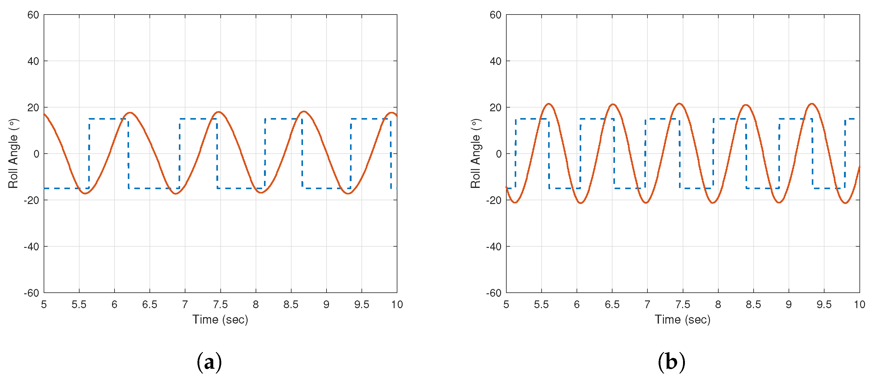
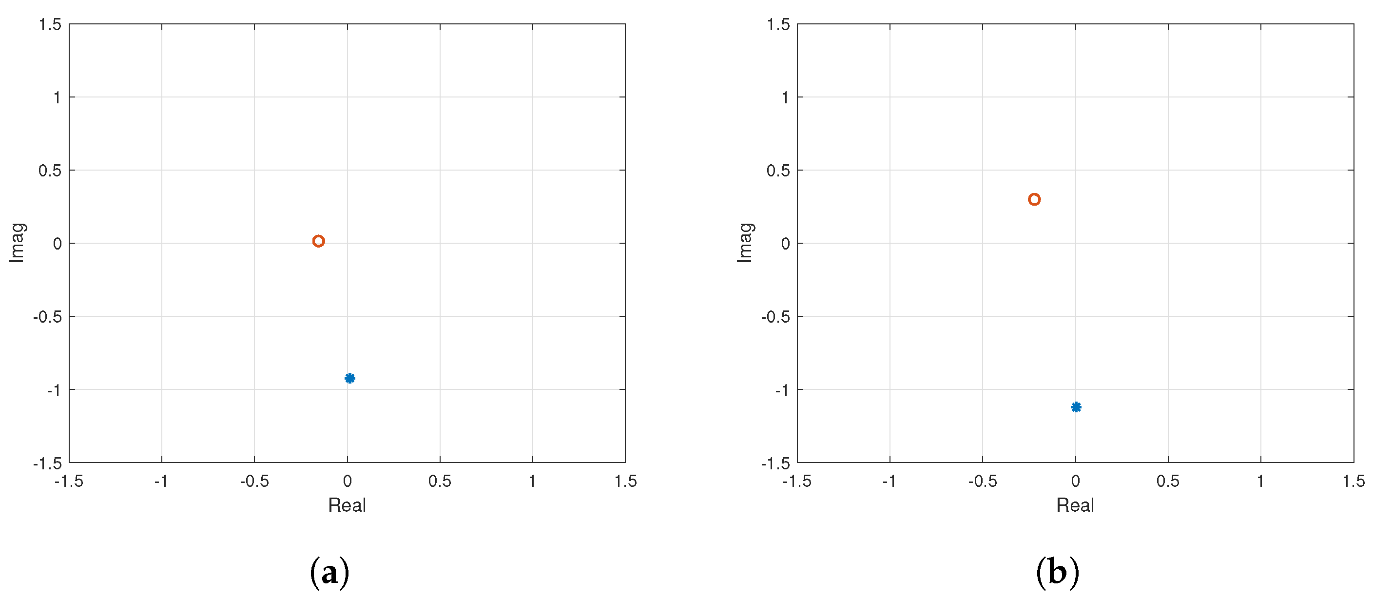
3.2. Relay Response Data Analysis Using FSF

When a system is driven by the relay with integrator apparatus, it produces an oscillatory response, as shown in Figures 6 and 10. For periodic output, fundamental discrete frequency is described by as ${\omega }_d=2\pi /N$ where N is the number of samples per cycle. Let $G\left(0\right)$ and $G\left(e^{\left(j{\omega }_d\right)l}\right)$ be the frequency response points of plant under relay experiment, then the relationship between the output $y\left(k\right)$ and input $u\left(k\right)$ using a frequency sampling model is given as in [56].

$$y\left(k\right)=G\left(0\right)f^0\left(k\right)+\sum _{l=-m}^{m}G\left(e^{\left(j{\omega }_d\right)l}\right)f^l\left(k\right)+v\left(k\right)$$

(6)

where $l=1,2,3,\cdots N$ and $m=(N-1)/2$. Here, $f^l\left(k\right)$ is known as FSF output vector and is defined as:

$$f^l\left(k\right)=\frac{1-q^{-N}}{N(1-q^{-1}{e}^{\left(j{\omega }_d\right)l})}u\left(k\right)$$

(7)

Here, $q^{-1}$ is a back-shift operator such that if $d\left(n\right)$ is a discrete time signal, $q^{-1}d\left(n\right)=d(n-1)$. In case of $l=0$, i.e., filter output at zero frequency, Equation (7) becomes

$$f^0\left(k\right)=\frac{1-q^{-N}}{N(1-q^{-1})}u\left(k\right)$$

(8)

The value of N is found by solving discrete Fourier transform of the input signal since it is periodic in nature. Afterward, the first sample with significant magnitude against its respective frequency point ${\omega }_d$ is selected to calculate $N=2\pi /{\omega }_d$ to the closest integer [57]. The term $v\left(k\right)$ in Equation (6) is used to incorporate noisy signal into the calculations. The distribution of noise is assumed to be Gaussian, with zero mean and variance ${\sigma }^2$. Moreover, the magnitude of the filter output diminishes as higher-order terms are computed for most of the processes. Given this inverse relationship between $f^l\left(k\right)$ and $\left|l\right|$, only few initial values of l are considered. Keeping this in consideration, Equation (6) is approximated as

$$\begin{array}{cc}\hfill y\left(k\right)& \approx G\left(0\right)f^0\left(k\right)+G\left(e^{j{\omega }_d}\right)f^1\left(k\right)+G\left(e^{-j{\omega }_d}\right)f^{-1}\left(k\right)+G\left(e^{2j{\omega }_d}\right)f^2\left(k\right)\hfill \\ \hfill & +G\left(e^{-2j{\omega }_d}\right)f^{-2}\left(k\right)+G\left(e^{3j{\omega }_d}\right)f^3\left(k\right)G\left(e^{-3j{\omega }_d}\right)f^{-3}\left(k\right)+v\left(k\right).\hfill \end{array}$$

(9)

A perfect periodic output signal is rarely acquired because of noisy measurements and other effects such as nonlinearity. This creates weaker even frequencies along with strong odd frequencies, as described by Fourier analysis [58]. An efficient estimation must also incorporate the effect of the weaker frequencies. Equation (9) considers the values with magnitudes close to zero through the inclusion of even terms. Therefore, it can be applied to relay feedback experiments that yield imperfect periodic output signals. Additionally, vectors presenting complex parameters and its correlating regressor vector are presented in Equations (10) and (11).

$$\begin{array}{c}\hfill \mathsf{\Theta }={\left[G\left(0\right)G\left(e^{j{\omega }_d}\right)G\left(e^{-j{\omega }_d}\right)G\left(e^{2j{\omega }_d}\right)G\left(e^{-2j{\omega }_d}\right)G\left(e^{3j{\omega }_d}\right)G\left(e^{-3j{\omega }_d}\right)\right]}^{*}\end{array}$$

(10)

$$\begin{array}{c}\hfill \mathrm{\Phi }={\left[f^0\left(k\right)f^1\left(k\right)f^{-1}\left(k\right)f^2\left(k\right)f^{-2}\left(k\right)f^3\left(k\right)f^{-3}\left(k\right)\right]}^{*}\end{array}$$

(11)

where ‘*’ represents the transpose of complex conjugate of variable under consideration. In order to compute the estimated frequency parameter vector, i.e., $\widehat{\mathsf{\Theta }}\left(k\right)$ as given by Equation (13), the recursive least square (RLS) algorithm can be used. A conventional way to write the RLS algorithm is given by Equation (12), also known as a covariance matrix.

$$\begin{array}{c}\hfill P\left(k\right)=P(k-1)-\frac{P(k-1)P{(k-1)}^{*}\mathrm{\Phi }\left(k\right)\mathrm{\Phi }{\left(k\right)}^{*}}{1+P(k-1)\mathrm{\Phi }\left(k\right)\mathrm{\Phi }{\left(k\right)}^{*}}\end{array}$$

(12)

$$\begin{array}{c}\hfill \widehat{\mathsf{\Theta }}\left(k\right)=\widehat{\mathsf{\Theta }}(k-1)+P(k-1)\mathrm{\Phi }\left(k\right)\{y\left(k\right)-\mathrm{\Phi }{\left(k\right)}^{*}\widehat{\mathsf{\Theta }}(k-1)\}\end{array}$$

(13)

Initial values required in equations above, i.e., $P\left(k\right)$ and $\widehat{\mathsf{\Theta }}\left(k\right)$ have been manually provided as $P(-1)$ and $\widehat{\mathsf{\Theta }}\left(0\right)$.

3.3. Automatic Tuning of PID Controller

When it comes to controller design, there are two basic requirements which are (1) the information of the system’s original behavior and (2) the information about the system’s desired behavior. These requirements can be available in the form of frequency response points, polynomials or transfer functions, etc. The concept of automatic tuning points towards a method that shapes the controller values through an automatic and simplistic way by utilizing the information of the plant’s original dynamics in the perspective of the desired behavior.

Step (1) Plant’s behavior:

In order to design a PID controller of the form $C\left(s\right)=\frac{c_2{s}^2+c_{1}s+c_o}{s}$, we need at least information of the system concerning at least two points on the Nyquist plot. That is, the first point in frequency response ${\omega }_1$ enables evaluation of $Kc$ and ${\tau }_i$, while ${\tau }_D$ is obtained using the second point ${\omega }_2$ in the frequency response data. With this in mind, consider that the frequency response of the plant at two frequency points ${\omega }_1$ and ${\omega }_2$ is known as $G\left(j{\omega }_1\right)$, $G\left(j{\omega }_2\right)$ [32,48]. When combined with PID controller transfer function in open-loop consideration, it yields $L\left(j\omega \right)$ such that:

$$\begin{array}{c}\hfill L\left(j\omega \right)=C\left(j\omega \right)G\left(j\omega \right)\end{array}$$

(14)

For two frequencies ${\omega }_1$ and ${\omega }_2$, the same can be given as

$$L\left(j{\omega }_1\right)=\frac{c_2{\left(j{\omega }_1\right)}^2+c_1\left(j{\omega }_1\right)+c_0\left(j{\omega }_1\right)}{j{\omega }_1}G\left(j{\omega }_1\right),$$

(15)

$$L\left(j{\omega }_2\right)=\frac{c_2{\left(j{\omega }_2\right)}^2+c_1\left(j{\omega }_2\right)+c_0\left(j{\omega }_2\right)}{j{\omega }_2}G\left(j{\omega }_2\right).$$

(16)

Step (2) Desired behavior:

The essence of any autotuner design lies within the process and complexity involved in the selection of the desired response. The purpose of the proposed autotuner is not only to achieve robust performance, but also is to keep the process simple. Therefore, the selection of desired performance is performed through the control sensitivity function of the first order as given below,

$$S_u\left(s\right)=\frac{1}{K_p}\times \frac{\frac{{\tau }_{cl}}{\beta }s+1}{{\tau }_{cl}s+1}$$

(17)

where $K_p$ is the steady-state gain of a plant, ${\tau }_{cl}$ is the desired closed-loop time constant and $\beta$ is the performance parameter used to calculate ${\tau }_{cl}$ from an known open-loop time constant (${\tau }_{op}$) of plant such that ${\tau }_{cl}=\beta {\tau }_{op}$. The value of $\beta$ must be carefully chosen such that $\frac{{\tau }_{cl}}{\beta }>0$ and $\frac{{\tau }_{cl}}{\beta }\approx$ dominant time constant of the system. It is obvious from Equation (17) that there is an inverse relationship between $\beta$ and the performance of the system, i.e., the high value of $\beta$ will result in slower performance and vice versa.

With the knowledge $K_p,{\tau }_{cl}$ and $\beta ,$ one can set the desired performance of system using Equation (17). In order to obtain these parameters, the suggested method utilizes the information obtained from the relay experiment. As the relay experiments proposed here use an embedded integrator, it can be verified through simple tests that the settling time of the plant can be approximated to $\frac{1}{2}N\mathsf{\Delta }t$, which is half of the integrated relay test cycle period (N) multiplied with sampling time ($\mathsf{\Delta }t$). Furthermore, the dominant time constant of the plant is set as one-fifth of this settling time obtained as follows:

$$\begin{array}{c}\hfill {\tau }_{op}=\frac{1}{5}\times \left(SettlingTime\right)=\frac{0.5N\mathsf{\Delta }t}{5}.\end{array}$$

Consequently, the sensitivity function $S_u\left(s\right)$ becomes:

$$\begin{array}{c}\hfill S_u\left(s\right)=\frac{0.1N\mathsf{\Delta }ts+1}{(0.1\beta N\mathsf{\Delta }ts+1)K_p}\end{array}$$

(18)

To obtain the consistent gain value $K_p$, direct calculation of the magnitude of plant’s frequency response is preferred along with the sign of unknown steady-state gain ($K_{ss}$) of the system as under

$$\begin{array}{c}\hfill K_p\approx sign\left(K_{ss}\right)\left|G_p\left(j{w}_1\right)\right|.\end{array}$$

The control sensitivity function $S_u\left(s\right)$ is merged with plant information $G\left(s\right)$ to generate a complementary sensitivity function $T_d\left(s\right)$ as given below

$$\begin{array}{c}\hfill T_d\left(s\right)=S_u\left(s\right)G\left(s\right),\end{array}$$

$$\begin{array}{c}\hfill T_d\left(s\right)=\frac{0.1N\mathsf{\Delta }ts+1}{0.1\beta N\mathsf{\Delta }ts+1}\left(\frac{G_p\left(s\right)}{K_p}\right).\end{array}$$

(19)

Equation (19) sets the desired response of the system with the help of the control sensitivity function. In order to compare the desired response with actual plant open-loop response given by Equations (15) and (16), the transfer function given by Equation (19) has to be converted into open-loop desired response ($L_d\left(j\omega \right)$), hence:

$$L_d\left(j\omega \right)=\frac{T_d\left(j\omega \right)}{1-T_d\left(j\omega \right)}$$

(20)

With the help of available information in the form of actual plant response given by Equation (14) and the desired response given by Equation (20), PID parameters are calculated by equating and comparing the responses as $L\left(j{\omega }_1\right)=L_d\left(j{\omega }_1\right)$ and $L\left(j{\omega }_2\right)=L_d\left(j{\omega }_2\right)$, we obtain

$$c_0=c_2{\omega }_1^{2}Real\left[X\left(j{\omega }_1\right)\right],$$

(21)

$$c_1=\frac{Imag\left[X\left(j{\omega }_1\right)\right]}{{\omega }_1},$$

(22)

$$c_2=\frac{Real\left[X\left(j{\omega }_2\right)\right]-Real\left[X\left(j{\omega }_1\right)\right]}{{\omega }_1^2-{\omega }_2^2}.$$

(23)

where $X\left(j{\omega }_1\right)=\frac{j{\omega }_1{L}_d\left(j{\omega }_1\right)}{G\left(j{\omega }_1\right)}$ and $X\left(j{\omega }_2\right)=\frac{j{\omega }_2{L}_d\left(j{\omega }_2\right)}{G\left(j{\omega }_2\right)}$. The classical PID values are obtained via $c_1,c_2$ and $c_0$ as given below,

$$K_c=c_1,{\tau }_i=\frac{c_1}{c_0},{\tau }_D=\frac{c_2}{c_1}.$$

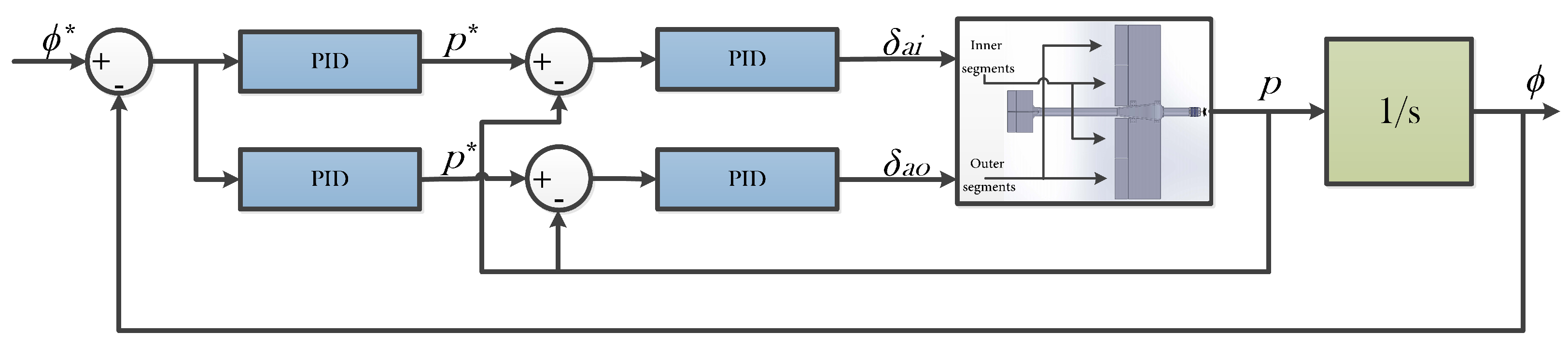
4. Cascade Control System for Roll Attitude Control

The objective of the control system of the multi-segmented aircraft is to control its roll angle attitude and follow the reference signal. The proposed control structure uses two cascade loops, i.e., the inner and outer loop. The inner loop is set to handle the roll rate of aircraft and is tuned to act much faster than the outer loop, which controls the roll angle. The benefit of this configuration becomes apparent in the event of a disturbance, where a fast-acting inner loop takes immediate disturbance rejection actions before it affects the roll angle of the aircraft.

4.1. Inner Loop Controller Development

To proceed with the design of roll rate control loop (inner loop), the relay with embedded integrator experiments are performed for both the inner and outer segments. Figure 6a,b show the time domain response of the inner and outer segments when subjected to relay tests. The amplitude of the relay with integrator apparatus used in experiments is maintained as equal to ${15}^{\circ }$.

The responses of the inner and outer segments are passed through the frequency sampling filter (FSF) to obtain the frequency response of systems. As detailed in the working methodology of the FSF filter, its output contains an array of estimated frequency response values ranging from the most dominant to the least dominant component in response. The relay experiment leads to one frequency response point, but from the estimated output array of the FSF filter, two points are selected. These points are denoted by $G_{pi}\left(j{\omega }_1\right)$ and $G_{pi}\left(j{\omega }_2\right)$ for inner segments and $G_{po}\left(j{\omega }_1\right)$ and $G_{po}\left(j{\omega }_2\right)$ for outer segments, as shown by Figure 7.

$$\begin{array}{c}\hfill G_{pi}\left(j{\omega }_1\right)=0.008099-0.04261j;G_{pi}\left(j{\omega }_2\right)=-0.125-0.0117j\end{array}$$

(24)

$$\begin{array}{c}\hfill G_{po}\left(j{\omega }_1\right)=-0.0111-0.9155j;G_{po}\left(j{\omega }_2\right)=-0.292-0.0245j\end{array}$$

(25)

It is evident from Figure 7 that the response of the inner and outer segments is different. For better control of the system, each of these sets of segments, i.e., the inner and outer segments, is considered as a separate system. Therefore, separate controllers are required for inner and outer segments.

To begin with the inner loop for inner segments, we first take two points as given by Equation (24) such that $G_{pi}\left(j{\omega }_1\right)$ and $G_{pi}\left(j{\omega }_2\right)$ represent the 3rd and 7th frequency points in FSF output array. With the gain equal to $K_p=\left|G_{pi}\left(jw1\right)\right|$ and closed loop time constant ${\tau }_{cl}=\beta {\tau }_{op}=0.1\beta N\mathsf{\Delta }t$, the value of $\beta =0.4$ leads us to the following sensitivity function.

$$\begin{array}{c}\hfill S_u\left(j{\omega }_1\right)=\frac{\frac{1}{\beta }{\tau }_{cl}j{\omega }_1+1}{({\tau }_{cl}j{\omega }_1+1)K_p}=2.5553+0.8320j\end{array}$$

The complementary sensitivity function $T_d\left(j{\omega }_1\right)$ is calculated as under

$$\begin{array}{c}\hfill T_d\left(j{\omega }_1\right)=S_u\left(j{\omega }_1\right)G\left(j{\omega }_1\right)=0.3752-1.0822j.\end{array}$$

Open-loop desired response $L_d\left(j{\omega }_1\right)$ is calculated as

$$L_d\left(j{\omega }_1\right)=\frac{T_d\left(j{\omega }_1\right)}{1-T_d\left(j{\omega }_1\right)}=-0.5999-0.6931j.$$

Likewise, we calculate the second complementary sensitivity function $T_d\left(j{\omega }_2\right)$ using a similar sensitivity function for response at ${\omega }_2$ i.e., $G_{pi}\left(j{\omega }_2\right)$, which leads to the following open-loop desired response.

$$L_d\left(j{\omega }_2\right)=\frac{T_d\left(j{\omega }_2\right)}{1-T_d\left(j{\omega }_2\right)}=-0.3233-0.1199j$$

Now, with the information of $G_{pi}\left(j{\omega }_1\right)$ and $G_{pi}\left(j{\omega }_2\right)$ along with $L_d\left(j{\omega }_1\right)$ and $L_d\left(j{\omega }_2\right)$, one can proceed to the following controller values using the relationship given by Equations (21)–(23).

$$\begin{array}{c}\hfill C\left(s\right)=\frac{c_2{s}^2+c_{1}s+c_0}{s}=\frac{0.0512s^2+1.5990s+16.4329}{s}\end{array}$$

Similarly, the inner loop PID controller for outer segments is designed using two frequency response points $G_{po}\left(j{\omega }_1\right)$ and $G_{po}\left(j{\omega }_2\right)$, given by Equation (25). Using $\beta =0.2$, the inner loop controller for outer segments is found as under

$$\begin{array}{c}\hfill C\left(s\right)=\frac{c_2{s}^2+c_{1}s+c_0}{s}=\frac{0.0386s^2+0.8432s+8.1303}{s}.\end{array}$$

The classical values for the inner loop controllers of the inner and outer segments are given by

Table 4. Inner loop controller parameters.

Inner Segments	Value	Outer Segments	Value
$K_c$	$1.5990$	$K_c$	$0.8432$
${\tau }_I$	$0.0973$	${\tau }_I$	$0.1037$
${\tau }_D$	$0.0320$	${\tau }_D$	$0.0458$

. It must be noted that all of the PID controllers are equipped with a low-pass filter. The filter works along with derivative term and has the form of $\frac{1}{{\tau }_{f}s+1}$ where the value of ${\tau }_f=0.1$. The implementation of the PID controller for the inner loop of both inner and outer segments is presented in Figure 8 where $p^{*}$ is the roll rate reference, p is the roll rate output, and ${\delta }_a$—plant input for the inner or outer segments.

4.2. Outer Loop Controller Development

In order to establish the dynamics for the outer loop for both inner and outer segments, another relay test is performed while keeping the inner loop closed. The relay experiment setup for outer loop dynamics identification is presented in Figure 9 where $r^{*}=0$ is the reference input to the relay apparatus. The roll reference input to the outer loop or angular position control loop, denoted by ${\varphi }^{*}$, is generated by the relay, and the reference for the inner loop $p^{*}$ is obtained from a simple proportional controller with a gain of $K_T$. Since the outer loop is assumed to be stable, it has been kept equal to unity gain. It is worth mentioning that while conducting the outer loop relay experiment, the inner loop PID controllers were implemented as developed in the previous section (see Table 4). The relay with integrator test yields time domain data, as shown by Figure 10, for both inner and outer segments. It is found that outer loop response signals for both of the segments have longer time periods due to the inclusion of the dynamics from the inner loop and the outer plant.

Proceeding further, the data from Figure 10 are passed through FSF filter to obtain frequency response points. As discussed in the previous section, two frequency response points, the 3rd and the 7th, are considered for PID design, as shown in Figure 11. The numeric values for obtained response points are given in Equations (26) and (27) where $G_{pi}^{olp}\left(j\omega \right)$ and $G_{po}^{olp}\left(j\omega \right)$ indicate the outer loop plant response for the inner and outer segments, respectively.

$$\begin{array}{c}\hfill G_{pi}^{olp}\left(j{\omega }_1\right)=0.01435-0.924j{G}_{pi}^{olp}\left(j{\omega }_2\right)=-0.1548+0.01379j\end{array}$$

(26)

$$\begin{array}{c}\hfill G_{po}^{olp}\left(j{\omega }_1\right)=0.0047-1.122j{G}_{po}^{olp}\left(j{\omega }_2\right)=-0.2214+0.2988\end{array}$$

(27)

With the information of $G_{pi}^{olp}\left(j{\omega }_1\right)$ and $G_{pi}^{olp}\left(j{\omega }_2\right)$ along with $L_d\left(j{\omega }_1\right)$ and $L_d\left(j{\omega }_2\right)$, one can proceed to the following controller values using relationship given by Equations (21)–(23).

$$\begin{array}{c}\hfill C\left(s\right)=\frac{c_2{s}^2+c_{1}s+c_0}{s}=\frac{0.0059s^2+0.4401s+2.4235}{s}\end{array}$$

Similarly, the outer loop PID controller for outer segments is designed using two frequency response points $G_{po}^{olp}\left(j{\omega }_1\right)$ and $G_{po}^{olp}\left(j{\omega }_2\right)$, given by Equation (27). Using $\beta =9.0$, the inner loop controller for outer segments is found in the following way:

$$\begin{array}{c}\hfill C\left(s\right)=\frac{c_2{s}^2+c_{1}s+c_0}{s}=\frac{0.0000582s^2+0.0913s+0.8161}{s}.\end{array}$$

The classical values for the outer loop controllers of the inner and outer segments are presented in

Table 5. Outer loop controller parameters.

Inner Segments	Value	Outer Segments	Value
$K_c$	$0.4401$	$K_c$	$0.0913$
${\tau }_I$	$0.1816$	${\tau }_I$	$0.1119$
${\tau }_D$	$0.0134$	${\tau }_D$	$0.000638$

.

5. Hardware Validation of Autotuned Controllers in Cascade System

When the inner and outer loop controllers are ready for both inner and outer segments, cascade configuration is deployed to integrate the controllers as shown in Figure 12 where ${\varphi }^{*}$ is the desired reference angle input, $\varphi$ is angle output, ${\delta }_{ai}$ is aileron input to the inner segments and ${\delta }_{ao}$ is aileron input to the outer segments.

Initially, two separate experiments were conducted to test the performance of aircraft. First, the cascade loop configuration is applied only on the inner segments, while the outer segments are kept inactive, i.e., at 0 degrees. Afterwards, the PID controllers designed for outer segments are cascaded to test the performance of outer segments while keeping inner segments inactive. It should be kept in mind that the performance of the inner and outer segments is tested in two test flight environments, i.e., in laminar and turbulent airflow.

In laminar flow or smooth airflow, the UAV encounters practically no substantial external disturbance other than native turbulence intensity of the wind tunnel test section, which was around $0.1$–$0.5\%$. However, to test the aircraft’s performance in the presence of external disturbances, a turbulent environment is created. Figure 13 shows a special box placed upright in the path of incoming airflow to generate turbulence inside the wind tunnel’s test section. The flow of experiments conducted in the wind tunnel is presented in Figure 14.

5.1. Performance Evaluation: Inner Aileron Segments

The step response of the roll angle is shown by Figure 15a when only inner segments are activated in laminar air flow. Whereas, roll rate response of the UAV under similar conditions is presented in Figure 15b. It is evident from Figure 7 and Figure 11 that inner segments have lower gain and bandwidth than the outer ones; hence, there is always a trade-off between rise time and overshoots. By studying the control signal presented in Figure 16a,b, it can be observed that the inner segments are struggling to keep up with reference tracking, especially in the event of turbulence. While at $t=10,18$ and 26 s, the control signal reaches the saturation limits because of the large step changes, as shown in Figure 16a, during the laminar airflow, the situation is concerning during turbulent airflow. Figure 16b shows that the control signal spends most of the time at the extremes of the graph. This is a result of the inherent lower gain of the plant, i.e., the inner segments, as discussed earlier.

The experimental evaluation is repeated in a turbulent environment. When the UAV works in an environment that has wind gusts changing suddenly, the inner segments are found to be less effective due to a slower response time. Figure 17a,b show the roll angle and rate output during turbulent airflow. It must be noticed that the outer aileron pair is kept at $0^{\circ }$ during these experiments. The closed-loop responses from the experiments performed in laminar and turbulent airflow demonstrate that the inner aileron segments have the ability to control the roll motion of the UAV during step changes in the reference signal. While the experimental results show that roll angle tracking in a turbulent environment is not as effective as in laminar flow, the inner segments are still capable of maintaining the closed-loop stability.

5.2. Performance Evaluation: Outer Aileron Segments

In order to better analyze performance difference, the outer aileron segments were tested under a similar experimental setup as the one used in the inner aileron segments. The step response generated while the UAV relying on only outer segments is presented in Figure 18a,b. These roll angle and roll rate responses were recorded when the aircraft was subject to laminar airflow. During the laminar airflow, the outer segments perform almost identically to the inner segments, except for lesser overshoots being observed at $t=18$ s. Figure 19a presents the control signal behavior when the outer segments are working in normal flight conditions. An important change to notice here is that the the control signal is mostly working within the range of $-19\%<{\delta }_{ao}<+18\%$, whereas for inner segments, the control signal is in the range of $-40\%<{\delta }_{ai}<+20\%$. Moreover, the control signal ${\delta }_{ai}$ has quickly reached the saturation limits at every step change, while the outer segments control signal ${\delta }_{ao}$ as zero taps on saturation points during the whole experiment. This behavior suggests that the outer segments, in comparison with inner ones, have good potential for tackling the big reference step changes or incoming disturbances.

However, when the UAV confronts irregular airflow, the outer segments are also able to reject externally induced disturbance and sustain the closed-loop stable operation. The closed-loop roll angle and roll rate responses are depicted in Figure 20a,b, respectively, when only the outer segments are working in a turbulent airflow. Further analysis into the control signal reveals that the outer segments are not using their full capacity to achieve the goal of reference tracking even in the presence of turbulence intensity similar to that of inner segments experiments. Figure 19b depicts that the control signal for the outer segments has the longest stay at saturation limit, i.e., $+100\%$ within the range of $17<t<18$ s and that is because of the huge step-change in the reference signal which is from $-{30}^{\circ }$ to $+{30}^{\circ }$, i.e., of ${60}^{\circ }$.

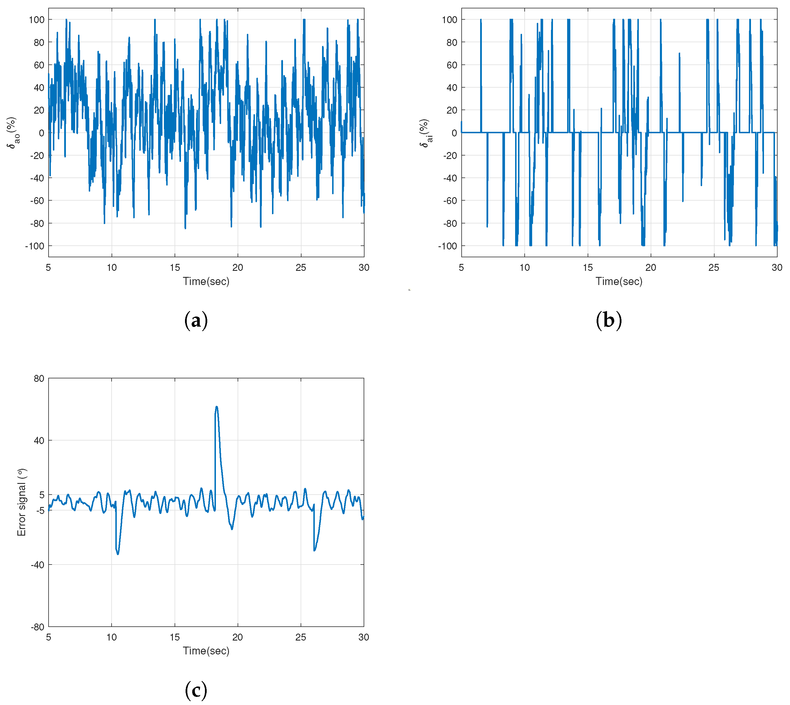
6. The Error-Threshold-Based Approach to Control of Segmented Surfaces

The detrimental impact of a windy and turbulent environment on a typical fixed-wing UAV is well acknowledged. Therefore, increasing the aileron size will require larger actuators that will affect the UAV’s reaction time and battery power when tackling severe turbulence. As a result, there will be additional difficulties that must be overcome, for instance, introducing the requirement for high-performance digital processors and expensive sensors. This aircraft deploys error-threshold-based aileron segment control in order to solve the problem. As was previously mentioned, the UAV in question has independent actuation capabilities on both its inner and outer aileron control surfaces. It is emphasized that only one pair of the ailerons should be active for reference tracking and rejection of insignificant disturbances in order to conserve battery energy during regular operation. The other pair of ailerons, in this case, the inner segments, is reserved as redundant ones. It is only active while rejecting powerful disturbances such as severe turbulence or improving reference following.

The control algorithm that determines whether the redundant pair of ailerons should be active or not relies on the intensity of external disturbance or the deviation of the UAV from given set-point. Since the external disturbance is directly linked with measured feedback error, i.e., the difference between reference roll angle denoted by ${\varphi }^{*}\left(t\right)$ and the UAV’s actual roll angle $\varphi \left(t\right)$, the large feedback error will call for involvement of all the aileron pairs to better stabilize the aircraft. Proceeding with this concept, the activation signal for multiple segments is formulated as,

$${\delta }_a\left(t\right)={\delta }_{ao}\left(t\right)+\lambda {\delta }_{ai}\left(t\right)$$

For the UAV used in this work, outer aileron segments are acting as primary actuators while inner ailerons are working as redundant ones. If the actuation threshold is defined by the pilot to be ${ϵ}_{act}$, then the error

$$|{\varphi }^{*}\left(t\right)-\varphi \left(t\right)|\le {ϵ}_{act}$$

will lead to $\lambda =0$, resulting in deactivation of inner ailerons. In the situation where error is

$$|{\varphi }^{*}\left(t\right)-\varphi \left(t\right)|>{ϵ}_{act}$$

the resulting $\lambda$ will be equal to 1, which will make inner segments active and work in support of outer aileron segments.

The value of ${ϵ}_{act}$ is user-selected and can vary based on an estimate of how turbulent an environment the UAV is going to fly in. All the experiments performed in this work are based on ${ϵ}_{act}=5^{\circ }$. Since the value of ${ϵ}_{act}$ is independent of PID controller values, depending upon user preferences, multiple thresholds such that ${ϵ}_{act}\in [5^{\circ },{10}^{\circ },{15}^{\circ }\dots ]$ can be programmed and triggered remotely using a flick of a switch. The independently tuned and deployed controllers for the inner and outer segments ensure that the lower the threshold, the better the disturbance rejection performance. Figure 21 represents the block diagram of the cascade controllers incorporating the error-threshold-based control. The switch before ${\delta }_{ai}$ can be treated like $\lambda$, hence, deciding whether the inner segments should be active or not.

The error-threshold-based control was tested in two flight environments. Figure 22a,b present the roll angle and roll rate outputs of aircraft while operating using the aforementioned control in the laminar airflow. The performance in this scenario resembles that of the outer segments since they are acting predominantly during the whole experiment. A slight improvement in the rise time can be noticed when looking at the points where step changes occur. This is because of the fact that the inner segments are active during the transition of the reference signal as $|{\varphi }^{*}\left(t\right)-\varphi \left(t\right)>5^{\circ }|$ and working in conjunction with outer segments to minimize the error as soon as possible. The working sequence of the inner and outer ailerons is made clear while looking at the control signals given in Figure 23. It is immediately observed from Figure 23a that the outer segments are normally active all the time within the average working capacity of $-19\%<{\delta }_{ao}<+18\%$. When compared to the individual performance of the outer segments where the overshoots were within the range of $-58\%<{\delta }_{ao}<+88\%$ (see Figure 19), the same ailerons are exhibiting lower overshoots at the reference step changes, i.e., within the range of $-30\%<{\delta }_{ao}<+39\%$ because of the assistance acquired from the inner segments. Figure 23c shows the error angle signal outlining the threshold band of $\pm 5^{\circ }$. Figure 23b presents the active and inactive time of the inner ailerons (${\delta }_{ai}$). By comparing Figure 23b,c, the error-threshold-based control can be observed in action such that the inner ailerons are only energized when the error signal has crossed the threshold limits, whereas, for rest of the time, they are held constant at ${\delta }_{ai}=0^{\circ }$.

The impact of the error-threshold-based control becomes clearer on the attitude performance as we proceed with experiments in a more challenging test environment. Figure 24 presents the attitude performance of the UAV in terms of the roll angle and rate while working in a turbulent airflow. It is noticed that the aircraft is able to sustain a smoother performance as compared to the previous experiments where only outer segments were active. A clear reduction in overshoots is observed, along with the proper tracking of roll angular rate, as shown in Figure 24b. The control signals and error signal behavior are depicted in Figure 25. The difference in working methodology of the inner segments is perceived in Figure 25b when compared to that of the laminar flow experiment. By analyzing the error signal given by Figure 25c, it is observed that the inner segments are active whenever the condition $|{\varphi }^{*}\left(t\right)-\varphi \left(t\right)>5^{\circ }|$ becomes true. This methodology ensures that there is no additional load on the limited onboard battery energy of the aircraft in a normal flight, and the improved performance is available at the discretion of the user or the challenging flight environment.

The mean squared error (MSE), which is calculated in order to better quantify the boost in the closed-loop performance of the hardware experiments conducted, is defined as $E=\frac{1}{M}{\sum }_{i=0}^{M-1}{({\varphi }^{*}\left(t_i\right)-\varphi \left(t_i\right))}^2$ where the number of samples is denoted by M. The MSE for the three distinct control configurations is depicted in

Table 6. Mean squared error (MSE): Performance analysis.

Aileron Configuration	MSE: Laminar Flow	MSE: Turbulent Flow
Inner segments only	$96.740$	$166.167$
Outer segments only	$75.100$	$153.099$
The error-threshold based control	$70.983$	$93.860$

. It can be inferred that the roll angle control response of the error-threshold based approach is superior by $6\%$ when compared to the independent performance of the outer ailerons only during laminar flow. Under similar conditions, the outer ailerons excel by a percentile of $22.3\%$ when compared to the independent working of the inner segments. However, the performance of the error-threshold-based control is much different from the individual actuation of either inner or outer segments in the presence of turbulence. The MSE analysis shows that the error-threshold-based control can offer a performance improvement of $38.69\%$ to $43.51\%$ while flying in a hostile environment.

7. Conclusions and Future Directions

This research work commences with system identification experiments utilizing a relay with embedded integrator to identify the aircraft’s dynamics. Two experiments were performed, one for the inner and another for the outer segments, to identify the unknown dynamics pertaining to the roll rate. Similarly, two more experiments were conducted to uncover the angular position dynamics. The information of the frequency response points is utilized immediately to tune the controllers using sensitivity functions and the performance parameter $\beta$. The hardware validation experiments are performed in RMIT’s wind tunnel under two test environments. The error-threshold-based control is proposed and implemented in hardware to achieve an extra degree of roll attitude stability. The experiments have manifested that the error-threshold-based control improves the roll attitude stability by a margin of $38.69\%$ to $43.51\%$ when compared to the independent actuation of aileron pairs in a turbulent atmosphere. While theoretically, the number of ailerons segments per side of the main wing can be unlimited, in practice, such a number must be carefully selected to avoid over-burdening of the main wing. Moreover, this work can be extended to explore the performance of the aileron segments on the leading edge of the main wing of UAV. Another promising future direction of this work can be in the selective disturbance rejection for small wind gust affecting only one side of the aircraft. Since the aileron segments have the capability to be actuated independently, the UAV can be equipped with lightweight air pressure sensors to detect pressure changes and selectively activate specific segments instead of triggering all actuators.

References

1. Cobleigh, B.R. Ikhana: A NASA UAS Supporting Long Duration Earth Science Missions; Technical Report, NASA TM-2007-214614; NASA Dryden Flight Research Center: Edwards, CA, USA, 2007.
2. Logan, M.; Chu, J.; Motter, M.; Carter, D.; Ol, M.; Zeune, C. Small UAV research and evolution in long endurance electric powered vehicles. In Proceedings of the AIAA Infotech@ Aerospace 2007 Conference and Exhibit, Rohnert Park, NV, USA, 7–10 May 2007; p. 2730. [Google Scholar]
3. Hernandez-Toral, J.L.; González-Hernández, I.; Lozano, R. Sun Tracking Technique Applied to a Solar Unmanned Aerial Vehicle. Drones 2019, 3, 51. [Google Scholar] [CrossRef] [Green Version]
4. Ackerman, E.; Koziol, M. The blood is here: Zipline’s medical delivery drones are changing the game in Rwanda. IEEE Spectrum 2019, 56, 24–31. [Google Scholar] [CrossRef]
5. Oakey, A.; Waters, T.; Zhu, W.; Royall, P.G.; Cherrett, T.; Courtney, P.; Majoe, D.; Jelev, N. Quantifying the Effects of Vibration on Medicines in Transit Caused by Fixed-Wing and Multi-Copter Drones. Drones 2021, 5, 22. [Google Scholar] [CrossRef]
6. Beard, R.W.; Kingston, D.; Quigley, M.; Snyder, D.; Christiansen, R.; Johnson, W.; McLain, T.; Goodrich, M. Autonomous vehicle technologies for small fixed-wing UAVs. J. Aerosp. Comput. Inf. Commun. 2005, 2, 92–108. [Google Scholar] [CrossRef] [Green Version]
7. Elbanhawi, M.; Mohamed, A.; Clothier, R.; Palmer, J.; Simic, M.; Watkins, S. Enabling technologies for autonomous MAV operations. Prog. Aerosp. Sci. 2017, 91, 27–52. [Google Scholar] [CrossRef]
8. Sun, J.; Tang, J.; Lao, S. Collision avoidance for cooperative UAVs with optimized artificial potential field algorithm. IEEE Access 2017, 5, 18382–18390. [Google Scholar] [CrossRef]
9. Yasin, J.N.; Mohamed, S.A.; Haghbayan, M.H.; Heikkonen, J.; Tenhunen, H.; Plosila, J. Unmanned aerial vehicles (uavs): Collision avoidance systems and approaches. IEEE Access 2020, 8, 105139–105155. [Google Scholar] [CrossRef]
10. Dainelli, R.; Toscano, P.; Gennaro, S.F.D.; Matese, A. Recent advances in Unmanned Aerial Vehicles forest remote sensing—A systematic review. Part II: Research applications. Forests 2021, 12, 397. [Google Scholar] [CrossRef]
11. Muñoz, J.; López, B.; Quevedo, F.; Monje, C.A.; Garrido, S.; Moreno, L.E. Coverage Strategy for Target Location in Marine Environments Using Fixed-Wing UAVs. Drones 2021, 5, 120. [Google Scholar] [CrossRef]
12. Khan, S.K.; Naseem, U.; Sattar, A.; Waheed, N.; Mir, A.; Qazi, A.; Ismail, M. UAV-aided 5G Network in Suburban, Urban, Dense Urban, and High-rise Urban Environments. In Proceedings of the 2020 IEEE 19th International Symposium on Network Computing and Applications (NCA), Cambridge, MA, USA, 24–27 November 2020; pp. 1–4. [Google Scholar]
13. Watkins, S.; Mohamed, A.; Fisher, A.; Clothier, R.; Carrese, R.; Fletcher, D.F. Towards autonomous MAV soaring in cities: CFD simulation, EFD measurement and flight trials. Int. J. Micro Air Veh. 2015, 7, 441–448. [Google Scholar] [CrossRef]
14. White, C.; Lim, E.; Watkins, S.; Mohamed, A.; Thompson, M. A feasibility study of micro air vehicles soaring tall buildings. J. Wind. Eng. Ind. Aerodyn. 2012, 103, 41–49. [Google Scholar] [CrossRef]
15. Mohamed, A.; Massey, K.; Watkins, S.; Clothier, R. The attitude control of fixed-wing MAVS in turbulent environments. Prog. Aerosp. Sci. 2014, 66, 37–48. [Google Scholar] [CrossRef]
16. Mohamed, A.; Clothier, R.; Watkins, S.; Sabatini, R.; Abdulrahim, M. Fixed-wing MAV attitude stability in atmospheric turbulence, part 1: Suitability of conventional sensors. Prog. Aerosp. Sci. 2014, 70, 69–82. [Google Scholar] [CrossRef]
17. Mohamed, A.; Watkins, S.; Clothier, R.; Abdulrahim, M.; Massey, K.; Sabatini, R. Fixed-wing MAV attitude stability in atmospheric turbulence—Part 2: Investigating biologically-inspired sensors. Prog. Aerosp. Sci. 2014, 71, 1–13. [Google Scholar] [CrossRef]
18. Mohamed, A.; Abdulrahim, M.; Watkins, S.; Clothier, R. Development and flight testing of a turbulence mitigation system for micro air vehicles. J. Field Robot. 2016, 33, 639–660. [Google Scholar] [CrossRef]
19. Abdulrahim, M. Flight dynamics and control of an aircraft with segmented control surfaces. In Proceedings of the 42nd AIAA Aerospace Sciences Meeting and Exhibit, Reno, NV, USA, 5–8 January 2004; p. 128. [Google Scholar]
20. Abdulrahim, M.; Lind, R. Investigating segmented trailing-edge surfaces for full authority control of a uav. In Proceedings of the AIAA Atmospheric Flight Mechanics Conference and Exhibit, Austin, TX, USA, 11–14 August 2003; p. 5312. [Google Scholar]
21. Boussalis, H.; Valavanis, K.; Guillaume, D.; Pena, F.; Diaz, E.U.; Alvarenga, J. Control of a simulated wing structure with multiple segmented control surfaces. In Proceedings of the 2013 21st Mediterranean Conference on Control and Automation (MED), Crete, Greece, 25–28 June 2013; pp. 501–506. [Google Scholar]
22. Wu, M.; Shi, Z.; Xiao, T.; Ang, H. Energy optimization and investigation for Z-shaped sun-tracking morphing-wing solar-powered UAV. Aerosp. Sci. Technol. 2019, 91, 1–11. [Google Scholar] [CrossRef]
23. Grant, D.; Abdulrahim, M.; Lind, R. Flight dynamics of a morphing aircraft utilizing independent multiple-joint wing sweep. In Proceedings of the AIAA Atmospheric Flight Mechanics Conference and Exhibit, Keystone, CO, USA, 21–24 August 2006; p. 6505. [Google Scholar]
24. Ifju, P.; Albertani, R.; Stanford, B.; Claxton, D.; Sytsma, M. Flexible-Wing Micro Air Vehicles; Mueller, T.J., Kellog, J.C., Ifju, P.G., Shkarayev, E.S., Eds.; WIT Press: Southampton, UK, 2006. [Google Scholar]
25. Ifju, P.; Waszak, M.; Jenkins, L. Stability and control properties of an aeroelastic fixed wing micro aerial vehicle. In Proceedings of the AIAA Atmospheric Flight Mechanics Conference and Exhibit, Montreal, QC, Canada, 6–9 August 2001; p. 4005. [Google Scholar]
26. Oduyela, A.; Slegers, N. Gust mitigation of micro air vehicles using passive articulated wings. Sci. World J. 2014, 2014, 598523. [Google Scholar] [CrossRef]
27. Martinez, R.M. Design and Analysis of the Control and Stability of a Blended Wing Body Aircraft. Master’s Thesis, Royal Institute of Technology (KTH), Stockholm, Sweden, 2014. [Google Scholar]
28. Zhao, A.; He, D.; Wen, D. Structural design and experimental verification of a novel split aileron wing. Aerosp. Sci. Technol. 2020, 98, 105635. [Google Scholar] [CrossRef]
29. Pena, F.; Martins, B.L.; Richards, W.L. Active In-flight Load Redistribution Utilizing Fiber-Optic Shape Sensing and Multiple Control Surfaces. NASA/TM-2018-219741. 2018. Available online: https://www.researchgate.net/publication/342533774_Active_In-flight_Load_Redistribution_Utilizing_Fiber-Optic_Shape_Sensing_and_Multiple_Control_Surfaces (accessed on 7 September 2022).
30. Lelaie, C. A380: Development of the flight controls Part: 1. In Safety First—The Airbus Safety Magazine. 2012. Available online: https://safetyfirst.airbus.com/app/themes/mh_newsdesk/documents/archives/a380-development-of-the-flight-controls.pdf (accessed on 7 September 2022).
31. Lelaie, C. A380: Development of the flight controls Part: 2. In Safety First–The Airbus Safety Magazine. 2012. Available online: https://safetyfirst.airbus.com/app/themes/mh_newsdesk/documents/archives/a380-development-of-the-flight-controls2.pdf (accessed on 7 September 2022).
32. Sattar, A.; Wang, L.; Mohamed, A.; Panta, A.; Fisher, A. System identification of fixed-wing uav with multi-segment control surfaces. In Proceedings of the 2019 Australian & New Zealand Control Conference (ANZCC), Auckland, New Zealand, 27–29 November 2019; pp. 76–81. [Google Scholar]
33. Moreira, E.I.; Shiroma, P.M. Design of fractional PID controller in time-domain for a fixed-wing unmanned aerial vehicle. In Proceedings of the 2017 Latin American Robotics Symposium (LARS) and 2017 Brazilian Symposium on Robotics (SBR), Curitiba, Brazil, 8–11 November 2017; pp. 1–6. [Google Scholar]
34. Poksawat, P.; Wang, L.; Mohamed, A. Automatic tuning of attitude control system for fixed-wing unmanned aerial vehicles. IET Control Theory Appl. 2016, 10, 2233–2242. [Google Scholar] [CrossRef]
35. Hervas, J.R.; Reyhanoglu, M.; Tang, H.; Kayacan, E. Nonlinear control of fixed-wing UAVs in presence of stochastic winds. Commun. Nonlinear Sci. Numer. Simul. 2016, 33, 57–69. [Google Scholar] [CrossRef]
36. Choi, M.H.; Shirinzadeh, B.; Porter, R. System identification-based sliding mode control for small-scaled autonomous aerial vehicles with unknown aerodynamics derivatives. IEEE/ASME Trans. Mechatron. 2016, 21, 2944–2952. [Google Scholar] [CrossRef]
37. Kang, Y.; Hedrick, J.K. Linear tracking for a fixed-wing UAV using nonlinear model predictive control. IEEE Trans. Control. Syst. Technol. 2009, 17, 1202–1210. [Google Scholar] [CrossRef]
38. Lam, V.T.T.; Sattar, A.; Wang, L.; Lazar, M. Fast Hildreth-based Model Predictive Control of Roll Angle for a Fixed-Wing UAV. IFAC-PapersOnLine 2020, 53, 5757–5763. [Google Scholar] [CrossRef]
39. Gomez, J.F.; Jamshidi, M. Fuzzy logic control of a fixed-wing unmanned aerial vehicle. In Proceedings of the World Automation Congress (WAC), Kobe, Japan, 19–23 September 2010; pp. 1–8. [Google Scholar]
40. de Oliveira, H.A.; Rosa, P.F.F. Genetic neuro-fuzzy approach for unmanned fixed wing attitude control. In Proceedings of the 2017 International Conference on Military Technologies (ICMT), Brno, Czech Republic, 31 May–2 June 2017; pp. 485–492. [Google Scholar]
41. Zhao, S.; Wang, X.; Kong, W.; Zhang, D.; Shen, L. A novel backstepping control for attitude of fixed-wing UAVs with input disturbance. In Proceedings of the 34th Chinese Control Conference (CCC), Hangzhou, China, 28–30 July 2015; pp. 693–697. [Google Scholar]
42. Kang, C.; Park, B.; Choi, J. Scheduling PID Attitude and Position Control Frequencies for Time-Optimal Quadrotor Waypoint Tracking under Unknown External Disturbances. Sensors 2022, 22, 150. [Google Scholar] [CrossRef]
43. Mystkowski, A. Robust control of the micro UAV dynamics with an autopilot. J. Theor. Appl. Mech. 2013, 51, 751–761. [Google Scholar]
44. Hoshu, A.A.; Wang, L.; Sattar, A.; Fisher, A. Auto-Tuning of Attitude Control System for Heterogeneous Multirotor UAS. Remote Sens. 2022, 14, 1540. [Google Scholar] [CrossRef]
45. Hoshu, A.A.; Wang, L.; Fisher, A.; Sattar, A. Cascade control for heterogeneous multirotor UAS. Int. J. Intell. Unmanned Syst. 2021. [Google Scholar] [CrossRef]
46. Hoshu, A.A.; Fisher, A.; Wang, L. Cascaded Attitude Control For Heterogeneous Multirotor UAS For Enhanced Disturbance Rejection. In Proceedings of the 2019 Australian and New Zealand Control Conference (ANZCC), Auckland, New Zealand, 27–29 November 2019; pp. 110–115. [Google Scholar]
47. Wang, L.; Cluett, W. Tuning PID controllers for integrating processes. IEE Proc.-Control. Theory Appl. 1997, 144, 385–392. [Google Scholar] [CrossRef]
48. Wang, L. PID Control System Design and Automatic Tuning Using MATLAB/Simulink; John Wiley & Sons: Hoboken, NJ, USA, 2020. [Google Scholar]
49. InvenSense. Embedded Motion Driver v5.1.1 APIs Specification; InvenSense Inc.: Sunnyvale, CA, USA, 2012. [Google Scholar]
50. Ravi, S. The Influence of Turbulence on a Flat Plate Aerofoil at Reynolds Numbers Relevant to MAVs. Ph.D. Thesis, School of Aerospace, Mechanical and Manufacturing Engineering, RMIT University, Melbourne, Australia, 2011. [Google Scholar]
51. Vino, G. An Experimental Investigation into the Time-Averaged and Unsteady Aerodynamics of the Simplified Passenger Vehicle in Isolation and in Convoys. Ph.D. Thesis, RMIT University, Melbourne, Australia, 2005. [Google Scholar]
52. Pagliarella, R. On the Aerodynamic Performance of Automotive Vehicle Platoons Featuring pre and Post-Critical Leading Forms. Ph.D. Thesis, RMIT University, Melbourne, Australia, 2009. [Google Scholar]
53. Beard, R.W.; McLain, T.W. Small Unmanned Aircraft: Theory and Practice; Princeton University Press: Princeton, NJ, USA, 2012. [Google Scholar]
54. Salman, S.A.; Sreenatha, A.G.; Choi, J.Y. Attitude dynamics identification of unmanned aircraft vehicle. Int. J. Control. Autom. Syst. 2006, 4, 782. [Google Scholar]
55. Sattar, A.; Wang, L.; Mohamed, A.; Fisher, A. Roll Rate Controller Design of Small Fixed Wing UAV using Relay with Embedded Integrator. In Proceedings of the 2020 Australian and New Zealand Control Conference (ANZCC), Gold Coast, Australia, 26–27 November 2020; pp. 149–153. [Google Scholar]
56. Wang, L. From Plant Data to Process Control: Ideas for Process Identification and PID Design; CRC Press: Boca Raton, FL, USA, 2014. [Google Scholar]
57. Wang, L. Automatic tuning of PID controllers using frequency sampling filters. IET Control Theory Appl. 2017, 11, 985–995. [Google Scholar] [CrossRef]
58. Kreyszig, E. Advanced Engineering Mathematics; John Wiley & Sons: Hoboken, NJ, USA, 2010. [Google Scholar]
Figure 1. The UAV model with dimensions.
Drones 06 00302 g001
Figure 2. UAV mounted on roll rig inside Industrial wind tunnel (IWT). (a) Top view showing flight controller board and sensors ➀ along with battery ➁. (b) Bottom view showing inner segments ➃,➄ and outer segments ➂,➅.
Drones 06 00302 g002
Figure 3. Flight controller with all I/O ports.
Drones 06 00302 g003
Figure 4. Setup of relay with integrator.
Drones 06 00302 g004
Figure 5. Location of fundamental frequency ( ω 1 ) when using relay with integrator.
Drones 06 00302 g005
Figure 6. Inner loop system identification for roll rate: Relay with embedded integrator experimental results for (a) Inner segments (b) Outer segments. Key: Dashed line shows relay excitation signal and solid line shows roll rate output.
Drones 06 00302 g006
Figure 7. Inner loop system identification for roll rate: Two frequency points extracted from relay output data for (a) Inner segments (b) Outer segments. Key: Stars indicate the 3rd and the circles indicate the 7th frequency response points.
Drones 06 00302 g007
Figure 8. Structure of inner loop with PID controller for roll rate control.
Drones 06 00302 g008
Figure 9. Relay test setup for outer loop identification.
Drones 06 00302 g009
Figure 10. Outer loop identification for roll angle: Relay with embedded integrator experimental results for (a) Inner segments (b) Outer segments. Key: Dashed line indicates relay excitation signal and solid line indicates roll rate output.
Drones 06 00302 g010
Figure 11. Outer loop identification for roll angle: Two frequency points extracted from relay output data for (a) Inner segments (b) Outer segments. Key: Stars show the 3rd and circles show the 7th frequency response points.
Drones 06 00302 g011
Figure 12. Cascade structure of inner and outer loops for roll angle control.
Drones 06 00302 g012
Figure 13. Wind tunnel setup for turbulence generation. (a) UAV facing incoming tubulent flow. (b) Closer look at turbulence generating box.
Drones 06 00302 g013
Figure 14. Sequence of experiments performed in the Wind Tunnel for Autotuned PID Controllers.
Drones 06 00302 g014
Figure 15. Inner segments during laminar flow. (a) Roll angle; (b) Roll rate output. Key: Dashed line indicates reference signal and solid line indicates output data.
Drones 06 00302 g015
Figure 16. Inner segments control ( δ a i ) input (a) during laminar airflow (b); during turbulent air flow.
Drones 06 00302 g016
Figure 17. Inner segments during turbulent flow. (a) Roll angle; (b) Roll rate output. Key: Dashed line indicates reference signal and solid line indicates output data.
Drones 06 00302 g017
Figure 18. Outer segments during laminar flow. (a) Roll angle; (b) Roll rate output. Key: Dashed line indicates reference signal and solid line indicates output data.
Drones 06 00302 g018
Figure 19. Outer segments control ( δ a o ) input (a) During laminar airflow (b) During turbulent air flow.
Drones 06 00302 g019
Figure 20. Outer segments during turbulent flow. (a) Roll angle; (b) Roll rate output. Key: Dashed line indicates reference signal and solid line indicates output data.
Drones 06 00302 g020
Figure 21. Cascade structure using error-threshold based control of the inner and outer segments.
Drones 06 00302 g021
Figure 22. The error-threshold based control in laminar flow. (a) Roll angle and (b) roll rate output. Key: Dashed line indicates reference signal and solid line indicates output data.
Drones 06 00302 g022
Figure 23. The error-threshold based control in laminar flow. (a) Control signal for the outer segment servos ( δ a o ). (b) Control signal for the inner segments ( δ a i ). (c) Angle error magnitude.
Drones 06 00302 g023
Figure 24. The error-threshold-based control in turbulent flow. (a) Roll angle (b) roll rate output. Key: Dashed line indicates reference signal and solid line indicates output data.
Drones 06 00302 g024
Figure 25. The error-threshold-based control in turbulent flow (a) Control signal for outer segment servos ( δ a o ); (b) Control signal for the inner segments ( δ a i ); (c) Angle error magnitude.
Drones 06 00302 g025