Classifying Forest Structure of Red-Cockaded Woodpecker Habitat Using Structure from Motion Elevation Data Derived from sUAS Imagery

Abstract

Small unmanned aerial systems (sUAS) and relatively new photogrammetry software solutions are creating opportunities for forest managers to perform spatial analysis more efficiently and cost-effectively. This study aims to identify a method for leveraging these technologies to analyze vertical forest structure of Red-cockaded Woodpecker habitat in Montgomery County, Texas. Traditional sampling methods would require numerous hours of ground surveying and data collection using various measuring techniques. Structure from Motion (SfM), a photogrammetric method for creating 3-D structure from 2-D images, provides an alternative to relatively expensive LIDAR sensing technologies and can accurately model the high level of complexity found within our study area’s vertical structure. DroneDeploy, a photogrammetry processing app service, was used to post-process and create a point cloud, which was later further processed into a Canopy Height Model (CHM). Using supervised, object-based classification and comparing multiple classifier algorithms, classifications maps were generated with a best overall accuracy of 84.8% using Support Vector Machine in ArcGIS Pro software. Appropriately sized training sample datasets, correctly processed elevation data, and proper image segmentation were among the major factors impacting classification accuracy during the numerous classification iterations performed.

1. Introduction

As small unmanned aerial system (sUAS) methods and technologies become increasingly more affordable, they are well poised to shift the way land and wildlife managers conduct data acquisition [1,2,3]. In forestry applications, sUAS platforms present opportunities to reduce operating cost and increase data precision by substituting for more traditional methods [4,5,6,7]. With sUAS methods, personnel needs are lowered, larger datasets are obtained faster, and limiting factors such as harsh terrain are not as impactful when compared to ground survey approaches.

sUAS are particularly advantageous when assessing forest classes and structure in fine detail [5]. Finer resolutions than 1 cm are possible, depending on flight configurations. Temporal scale is also relatively unrestricted, with sUAS technologies easily and quickly deployable [8]. This makes sUAS approaches a relatively cost-effective and flexible data acquisition option when compared to alternatives such as manned flight or satellite remote sensing methods [7].

Decentralization of forest management from government to smaller communities is an important trend that works in the interest of forest conservation [9]. Numerous countries are currently or beginning to adopt this structure of forest governance because of the benefits of empowering community or municipal level forest managers [10,11,12]. Successful forest governance looms large in the climate change agenda, with deforestation and loss of biodiversity being factors to consider [13]. Affordable and accessible forest monitoring methods are an invaluable tool to these communities of forest managers, many of whom are already leveraging sUAS technologies to acquire data and perform analysis [14,15,16,17]. Opportunities to reinforce the capabilities of these technologies and expand on their applications will only continue to enable forest managers who conduct data acquisition with limited resources.

Standout methods for assessing vertical structure of forested areas include Structure from Motion (SfM) and LIDAR, or light detection and ranging, with multiple examples of comparisons in the literature [18,19,20,21]. SfM uses photogrammetry algorithms and numerous overlapping photos to model vegetation structure, whereas LIDAR sends and receives light pulses for measuring “ranges” in the study area. Both methods generate a 3-dimensional point cloud representing vegetation structure. This is then used to assess a variety of forest indices, such as tree height, stand inventorying, or biomass measurements [6,22,23]. While LIDAR has shown to be an effective approach for penetrating past the upper canopy to evaluate vertical forest structure, it is a relatively expensive method when compared to SfM.

The use of low-cost sUAS technologies has already been leveraged in other successful studies where SfM served as a feasible method of point cloud generation [21,24,25,26,27]. SfM was employed in New South Wales to highlight the benefits and capabilities of photogrammetric methods for detecting sirex-attacked trees, and monitoring forest health remotely [25]. Color orthophotos proved to be an effective tool in this case, especially when paired with a near-infrared band. Information as discrete as tree species was identified in another study, where supervised classification using a Random Forests classifier was performed to identify various tree species along multiple phenological timelines [26]. The Red-Green-Blue color bands, the same acquired by most consumer-grade cameras, proved to be more effective at species identification than near-infrared sensing in this study. Another study used multi-temporal crop surface models (CSMs) to derive barley plant height (PH), and later estimate crop biomass using PH and linear modeling [27]. These technologies are highly adaptable, and can be applied to a variety of research questions. In our case, we sought to use SfM combined with a consumer-grade sUAS to assess red-cockaded woodpecker habitat.

Red-cockaded woodpeckers (Dryobates borealis) are currently listed as an endangered species by the U.S. Fish and Wildlife Service, and are endemic to the Southeastern United States [28,29,30]. One of the primary characters defining high-quality red-cockaded woodpecker (RCW) habitat is old pine trees for roosting and nesting cavity excavation; preferably Longleaf Pine (Pinus palustris) or Shortleaf Pine (Pinus echinate), followed by Loblolly Pine (Pinus taeda) or Slash Pine (Pinus elliotii), although their presence, absence, and ratios can vary by region and management history [28,29,30,31,32]. Other factors determining habitat quality include herbaceous groundcover, intermediate pine density, and absence of midstory, all of which are positive contributors to RCW fitness [28,30,32]. These three habitat features are also positively correlated with the use of prescribed fire, particularly growing season fires, as a management tool [28,30,32]. Frances C. James et al. concluded that the density of larger trees (>35 cm diameter at breast height (dbh)) compared to smaller trees (15–25 cm dbh), and also the ratio of herbaceous ground cover to woody ground cover, are both major contributors to RCW fitness [33]. Another study by France C. James et al. suggests that, in addition to ground cover composition, the extent of natural pine regeneration was also significantly related to the birds’ success and therefore habitat quality [34].

What previous studies have made clear is that the distribution of these various forest classes and their abundance are major indicators of RCW habitat quality. There are some examples where LIDAR technologies were used to asses the vegetative structure of RCW habitat or similar habitat [35,36]. In this case, SfM will be used as a low-cost, low-complexity alternative for RCW habitat assessment. Of particular interests are the habitat quality indicators mentioned above; herbaceous ground cover, the prescence of woody midstory, the amount of pine regeneration, and the amount of mature or overstory pine.

2. Materials and Methods

2.1. Study Area

From March 2020 through March 2021, Raven Environmental Services conducted multiple prescribed burns in and around Unit 0607 on Cook’s Branch Conservancy, or CBC, in Montgomery County, Texas. The fire resulted in areas of pine overstory loss and scorching of overstory and midstory pine. Dominant forest species include mature individuals of Loblolly Pine with some mature Shortleaf Pine, and small amounts of deciduous species including Southern Red Oak (Quercus falcata), Black Hickory (Carya texana), and Farkleberry (Vaccinium arboreum). Understory consists of mostly Yaupon Holly (Ilex vomitoria) and American Beautyberry (Callicarpa americana). Major herbaceous ground cover species include Little Bluestem (Schizachyrium scoparium) and Longleaf Wood Oats (Chasmanthium sessiliflorum). Long-term forest management goals aim to preserve and foster a target amount of natural pine regeneration to serve as a future generation and source of cavity trees for red-cockaded woodpeckers that inhabit the area. Because CBC’s surrounding area is becoming rapidly more urbanized in recent years, it is important that forested areas maintain a long-term perspective by inventorying pine regeneration.

A summary of this study’s workflow can be found in Figure 1, and is broken into imagery collection, processing imagery in DroneDeploy, and analysis in both eCognition and ArcGIS Pro.

2.2. Imagery Capture

Capture of imagery was facilitated by a sUAS that weighs under 24.9 kg, and therefore subject to the Federal Aviation Administration Part 107 Rules and Regulations. Tailored for small, commercial use, this regulatory system is relatively simple in its compliance requirements. A software app service named DroneDeploy that provides photogrammetric services was used to create an orthophoto from over 2000 nadir photographs taken during flight missions. DroneDeploy, along with other photogrammetry cloud services such as Pix4D, have and continue to provide access to affordable and low-complexity photogrammetry options [37,38].

The sUAS used was a consumer-grade DJI Mavic Pro Platinum with a monocular camera (DJI-FC220 sensor) capturing imagery in the Red-Green-Blue (RGB) color bands. The initial study area was 120 hectares, and flight time was approximately 4–5 h on Thursday, 4 March 2021. DroneDeploy’s mission planning services created a predetermined and editable grid above the study area that the sUAS followed while capturing imagery. Transects maintained an approximate east-to-west bearing, total images captured was 1890, and image resolution was 2.57 cm/px. The area was too large to capture during one battery lifecycle, so multiple flight missions were flown throughout the day. A summary of flight details is found in

Table 1. Summary of flight details.

Project Name	0600–Map Plan
Photogrammetry Engine	DroneDeploy Proprietary
Date of Capture	4 March 2021
Date Processed	11 March 2021
Processing Mode	Standard
GSD Orthomosaic (GSD DEM)	2.57 cm/px (DEM 10.29 cm/px)
Area Bounds (Coverage)	1,206,020 m2
Image Sensors	DJI–FC220

, and the flight path and imagery capture points are presented in Figure 2.

The timing of imagery capture was intentionally selected during dormant season so that deciduous trees were in a leaf-off state. This allowed for better discrimination of hardwood species from pine species. Figure 2 also illustrates the quality of coverage and where GPS alignment issues occurred. Areas symbolized with yellow boxes and red X’s correlated with issues in elevation data seen later.

2.3. Processing Imagery Using DroneDeploy

Following imagery capture, photos were uploaded to DroneDeploy’s website where photogrammetric processing occurs in their cloud environment. Processing of photos took approximately an hour, and exported data included an orthoimage (Figure 3), a digital terrain model (DTM) (Figure 4), and a point cloud with a point density of 10.44 points/m² (Figure 5). Exportable options include various file types and projected coordinate systems. For this study, .tiff file types were used for the DTM and orthoimage, a .las file type was used for the point cloud, and all of the data were exported using a NAD 1983 UTM Zone 15 projected coordinate system.

2.4. Classification Configuration and Classifier Selection

Forest classification methods are numerous, and primarily consist of object or pixel-based, supervised or unsupervised, and parametric or non-parametric machine learning classifiers [39,40]. A variety of approaches have been employed, but more recent forest classification studies suggest that supervised, object-based classifications are favorable [26,41]. There is, however, ambiguity found when considering the optimal classifier to use, with several comparisons made of Random Forests (RF) (referred to as Random Trees (RT) in ArcGIS), Maximum Likelihood (ML), Support Vector Machine (SVM), K-Nearest Neighbor (KNN), and also deep learning algorithms, such as Convolutional Neural Networks (CNN) [39,40,42,43].

Supervised, object-based classification using both ArcGIS Pro and eCognition software packages was performed for this study. For both software options, results were compared when using SVM and RT classifiers, whereas other classifiers specific to either software option were also used. Those included ML in ArcGIS Pro, and KNN, Naïve Bayes, and Decision Tree (DT) in eCognition. Both ArcGIS Pro and eCognition provided processing tools for rasterizing point cloud data and normalizing surface elevation, but training and accuracy assessment samples created in ArcGIS Pro were used for analysis in both software products.

2.5. Classification in ArcGIS Pro

2.5.1. Reduction in Study Area and Normalizing Elevation Data in ArcGIS Pro

A workflow and model were then developed in ArcGIS Pro to arrive at a raster representing normalized elevation or a Canopy Height Model (CHM). This was done by converting the point cloud to raster format, and then subtracting those values by the DTM using a Raster Calculator tool.

The resulting CHM contained a large anomalous area that coincided with GPS alignment issues during sUAS flights, and seen in Figure 2, Figure 4 and Figure 5. Additionally, there appeared to be evidence that the stopping and starting of imagery capture, due to the need to change batteries, may have had an impact on the continuity of elevation data moving northward. These issues are highlighted by well-defined graduations in elevation data, seen occurring twice in the DTM in approximately the northern third of the study area (Figure 4). For this reason, a 27 hectare area of consistent and reliable elevation data was selected from the original study area to be used for analysis going forward (Figure 6).

The selected area was surveyed continuously, and without interruptions due to battery changes. Therefore, it also had more consistent luminosity features, in addition to elevation data. It also excludes the large, questionable area of elevation data, while almost completely including a continuous management unit. This reduction in study area also enabled faster processing time during subsequent analysis steps, which amounted to an overall significant time savings because of the large number of iterations performed.

2.5.2. ArcGIS Pro: Creation of CHM Classes and a Segmented Image

After clipping out the new study area, a histogram of the CHM was created (Figure 7). The distribution of height values is noticeably similar to the vegetative structure found in another where LIDAR was used [35]. In both cases, most of the distribution is found at lower elevations, with negligible amounts of negative values. This figure provides several insights into the vertical structure of the study area and how to organize classes.

Using the CHM histogram, and a comparison of the CHM and orthoimage, image interpretation was used to create height classes using the Reclassify Raster geoprocessing tool. Additionally considered were heights for major herbaceous ground cover species, and approximate heights for midstory and pine classes in similar studies.

Most of the pixels are found between −0.55 and 1.17 m, which is interpreted as pixels representing approximately ground level, basal vegetation, and woody debris laying on the ground (Figure 8). Because identifying herbaceous ground cover is of interest, and serves as a relevant metric for assessing RCW habitat, the heights of two major grass species in the study area were also factored into this height class. The first, Little Bluestem, has a culm height range of 7–210 cm, and the second, Longleaf Wood Oats, has a culm height range of 50–150 cm [44]. Therefore, an upper height of 117 cm will capture most of these two species occurrences.

Heights between 1.17 and 2.9 m were interpreted as shrub vegetation. Yaupon Holly is a common shrub species within the study area and does not lose its leafy vegetation during dormant season. Between its height profile and textural characters, it was frequently identified as making up this height class (Figure 8). Additionally, previous study describes “medium-quality” RCW habitat as having woody hardwood vegetation that is on average 2.7 m or shorter, so an upper threshold of 2.9 m is approximately within this threshold [32].

Midstory height classes consisted of 2.91–6.34, 6.35–9.79, and 9.80–11.51 m. Areas including all of these classes (2.91–11.51 m) typically represented pine regeneration, were often spatially large and contiguous, and height classes were largest in the central areas (Figure 8 and Figure 9). Pine trees with heights below 12 m are shown to provide significantly less RCW foraging potential than pines trees above 12 m, so an upper threshold of 11.51 m also serves to divide pine regeneration from older pine trees used for foraging or cavity trees [32].

Canopy levels represented pine overstory or hardwood, and were broken into two classes, 11.51–18.41 and 18.42–39.08 m. Similar studies of RCW habitat have maximum pine heights of 24.54 m in one example, and 27.1–30 m in another [32,35]. Our CHM histogram is similar, with the height distribution falling off abruptly at approximately 30 m (Figure 7). The histogram also provides some context for these height classes, with their distribution of pixels spread over several values. Additionally, the number of pixels decrease slightly as the heights increase, indicating that taller trees occur less frequently. The height profiles of pine overstory tended to be complex but conspicuously taller (Figure 8). This made sense intuitively, with the pixel resolution allowing for penetration past the tallest branches and into some of the more irregular and lower portions of a pine trees canopy. Figure 10 shows a finalized map of the CHM reclassification.

2.5.3. Image Segmentation

Image segmentation was performed using the Image Segmentation tool in ArcGIS Pro. Because of the orthoimage’s high complexity and fine pixel resolution, this process took several attempts before identifying the best parameters for segmentation. Ideally, a segmented image will represent discrete objects, while also representing them completely and separately from neighboring objects. This was best achieved when slightly reducing spectral detail and increasing spatial detail from the tool’s default settings. Minimum segment size in pixels was kept at the default setting of 20. Figure 11 illustrates a portion of the segmented image compared to its orthoimage counterpart.

2.5.4. Combining Segmented Image and CHM Bands

To incorporate both the segmented image and elevation data in the classification analysis, the two raster layers were combined using the composite bands geoprocessing tool. The resulting layer contained red, green, and blue bands, and a fourth band containing the study area’s reclassified CHM.

2.5.5. ArcGIS Pro: Creation of Forest Classes and Training Samples

A class schema was created and consisted of seven forest classes: Pine Overstory, Pine Regeneration, Scorched Pine Overstory, Scorched Pine Regeneration, Deciduous/Dead Pine, Shrub Layer, and Ground Cover. Deciduous trees and dead pine were grouped together because of their visual similarities, and because discriminating one from the other was not necessary for the purpose of this study.

Training samples were produced by overlaying the reclassified CHM and segmented image, and identifying areas where an image segment coincided with the appropriate elevation data. For example, a training sample for Pine Overstory would be selected where green canopy and the highest elevation values overlapped. Training samples were drawn in some cases, and in other cases, a segment selection tool was used. Ground Cover training samples were always drawn manually because when entire segments were selected, the classifier tended to overrepresent them. All the pine classes were appropriately represented using both segment selections or manually drawn training samples. The use of the segment selection tool greatly increased the efficiency and speed at which training samples were created. Effort was made to randomly distribute segments throughout the study area for each class, but for some classes this was difficult because of their sparse distribution. Scorched Overstory and Hardwood/Dead Pine were the best examples of this, with representatives being less frequent and their distribution uneven. Previous studies indicated that an insufficient amount of training samples for classifier training could have a negative impact on accuracy, with less than 125 greatly reducing accuracy [15]. With this number in mind, 1400 training samples were created for all 7 classes. They were divided into two groups; 1050 were used for training classifiers, and 350 were later used for accuracy assessment. Training samples were divided equally amongst classes, with 150 per class used for training classifiers, and 50 per class used for accuracy assessment. Figure 12 illustrates the distribution of training samples throughout the study area.

2.5.6. ArcGIS Pro: Classification

The Image Classification Wizard in ArcGIS Pro was used to train three classifiers: SVM, RT, and ML. Both SVM and RT are non-parametric classifiers, and ML is a parametric classifier. Object-based, supervised classification was selected for configuration. The previously mentioned classification schema of seven classes was added to the tool, along with the 1050 training samples (150 per class), and the RGB segmented image that included the reclassified CHM. SVM was configured to 500 samples per class, and RT was configured to a maximum of 50 trees, a maximum tree depth of 30, and a maximum of 1000 samples per class. ML did not require any specific configuration setup.

2.5.7. ArcGIS Pro: Accuracy Assessment

Once each map was generated, they were individually assessed for overall accuracy using an Accuracy Assessment tool and the 350 remaining training samples (50 per class) not used for training the classifiers. Stratified Random sampling was used, where accuracy assessment points were distributed randomly within each class, and with a number of points proportional to the overall pixel size of each class. Outputs for each classifier include a confusion matrix with accuracy per class, user accuracy, producer accuracy, overall accuracy, and Kappa Index.

2.6. Classification in eCognition

2.6.1. eCognition: Normalizing Elevation Data

Using eCognition software, the point cloud was rasterized using the average of Z-coordinates and a kernel size of 11 (Figure 13). A histogram of elevation values was also produced (Figure 14) and shows an almost identical distribution of elevation values when compared to the histogram produced in ArcGIS Pro (Figure 7). The kernel size parameter was compared to other trial settings and appeared to do the best job of smoothing outputs. Next, using the nDSM tool, the rasterized point cloud and DTM were inputted to produce a CHM. A median filter tool with a kernel size of 3 was then used on the CHM to remove outlier elevation values.

2.6.2. eCognition: Image Segmentation and Training Samples

Using the Multiresolution Segmentation tool, image segmentation was performed that considered the red, blue, and green bands (RGB) from the orthoimage, and the filtered CHM as a fourth band. Multiple iterations of this step using different parameters were performed to try to best identify a method for image segmentation. It was decided to use band weights of 2 for the RGB bands, and 0.5 for the CHM band. Image segmentation that weighed the CHM too heavily resulted in relatively low classification accuracies later. The scale parameter was set to 50, shape to 0.3, and compactness to 0.7.

The 1050 training samples created and used in ArcGIS Pro were now imported into eCognition as a thematic layer. Using the Assign Classes by Thematic Layer tool, the same class hierarchy was generated, including the Pine Overstory, Pine Regeneration, Scorched Pine Overstory, Scorched Pine Regeneration, Ground Cover, Hardwood/Dead Pine, and Shrub Layer classes. Next, the Classified Image Objects to Samples tool was used to take the image objects created from segmentation and create training samples for each class where the thematic layer and image objects overlapped (Figure 15).

These training samples were then saved as training sample statistics in a .csv file, and the class hierarchy removed. The 350 accuracy assessment samples used in ArcGIS Pro were then imported as a thematic layer, and the same steps performed for creating samples in eCognition. The intention here was to separate the saved training sample statistics for classification from the newly imported accuracy assessment samples.

2.6.3. eCognition: Classification

With image segmentation completed and training sample statistics saved, supervised, object-based classification was performed. Multiple classifier algorithms are available within the Supervised Classification tool in eCognition, some of which were not available in ArcGIS Pro. Classifiers used on both software packages were SVM and RT, and classifiers specific to eCognition used included Bayes, KNN, and DT.

A classification model was created, classifier parameters selected, and each of the classifiers were trained using the stored sample statistics. For KNN, K-values of both 3 and 5 were used in separate iterations. For RT and DT, minimum sample counts of 0 and a maximum number of 16 categories were used, and for RT specifically, 50 trees per node. When using SVM, a linear kernel type and C value of 2 were used.

2.6.4. Ecognition: Accuracy Assessment

Generating a confusion matrix in eCognition was done using the Accuracy Assessment tool and selecting “output of error matrix bases on sample statistics”. The image object level already has the accuracy assessment samples imported from previous steps, so the tool used them to generate results. This step was performed for each classifier.

3. Results

For ArcGIS Pro classifications, accuracy was highest using Support Vector Machine, followed by Random Trees, and least accurate using Maximum Likelihood. eCognition’s best classification results were produced by KNN, with the remaining classifier options producing relatively less accurate classifications when compared to their KNN counterpart and ArcGIS Pro results. SVM in eCognition was a significant outlier, with a poor overall accuracy. A summary of these results is seen in

Table 2. Overall accuracy and Kappa Index values for all the classifiers in both software packages.

Software	Classifier	Overall Accuracy	Kappa Index
ArcGIS Pro	ML	0.754	0.689
	RT	0.804	0.752
	SVM	0.848	0.805
eCognition	KNN	0.744	0.695
	Bayes	0.687	0.63
	DT	0.521	0.437
	RT	0.418	0.432
	SVM	0.123	0.008

:

3.1. Classification Maps and Confusion Matrices

The results of the top-performing classifiers in each software option are focused on specifically here; SVM in ArcGIS Pro and KNN in eCognition. Classification maps (Figure 16 and Figure 17) and confusion matrices (

Table 3. Support Vector Machine confusion matrix and classification results in ArcGIS Pro.

Class	Overstory	Regeneration	Overstory Scorched	Regeneration Scorched	Ground Cover	Deciduous/Dead Pine	Shrub Layer	Total
Overstory	50	2	7	0	1	0	1	61
Regeneration	2	49	0	0	0	0	0	51
Overstory Scorched	0	0	161	2	6	0	1	170
Regeneration Scorched	0	0	9	41	0	0	0	50
Ground Cover	2	1	11	0	91	0	1	106
Deciduous/Dead Pine	3	0	12	1	10	17	0	43
Shrub Layer	4	0	0	0	0	0	15	19
Total	61	52	200	44	108	17	18	500
Producer Accuracy	0.819672	0.942308	0.805	0.931818182	0.842593	1	0.833333
User Accuracy	0.819672	0.960784	0.947059	0.82	0.858491	0.395349	0.789474
Overall Accuracy	0.848
Kappa Index	0.805034

and

Table 4. K-Nearest Neighbor confusion matrix and classification results in eCognition.

Class	Overstory	Regeneration	Overstory Scorched	Regeneration Scorched	Ground Cover	Deciduous/Dead Pine	Shrub Layer	Total
Overstory	307	62	27	20	55	31	20	522
Regeneration	6	284	7	15	9	6	1	328
Overstory Scorched	13	2	559	17	31	17	4	643
Regeneration Scorched	4	4	21	310	6	14	0	359
Ground Cover	20	13	27	8	404	78	58	608
Deciduous/Dead Pine	9	9	10	6	42	151	3	230
Shrub Layer	6	19	5	1	22	4	119	176
Total	365	393	200	377	569	301	205	2866
Producer Accuracy	0.841	0.7226463	0.8521341	0.8222812	0.71	0.5016611	0.5804878
User Accuracy	0.5881226	0.8658537	0.8693624	0.8635097	0.6644737	0.6565217	0.6761364
Overall Accuracy	0.74453918
Kappa Index	0.6953414

) provide more details about classification results. Visually, the major themes of both classification maps are similar, with larger-scale examples in each figure providing more conspicuous differences in outputs. One similar trend in both classifiers’ confusion matrices is the poor user accuracy for the Hardwood/Dead Pine class. User accuracy is relatively lower in the Pine Overstory, Ground Cover, and Shrub Layer classes when using KNN in eCognition. Conversely, KNN only marginally outperformed SVM in ArcGIS Pro in a few instances. Both classifiers performed well when classifying Pine Regeneration, Scorched Pine Regeneration, and Scorched Pine Overstory classes.

Classification maps and confusion matrices for the remaining ArcGIS Pro and eCognition classifiers can be found in the Appendix A section.

3.2. Area Calculations Using ArcGIS Pro Classification Results

Quantifying area per class was also performed by taking individual pixel area, multiplying it by pixel count per class, and converting area from square meters to hectares. ArcGIS Pro classification results were used to quantify area because of their relatively high accuracy results.

Table 5. Area per class in hectares, and percentage of coverage for each class.

	Area in Hectares			Percent Coverage
	ML	RT	SVM	ML	RT	SVM
Overstory	3.21	5.32	4.72	11.89%	19.73%	17.51%
Regeneration	4.46	4.03	4.04	16.56%	14.94%	14.99%
Overstory Scorched	1.28	1.42	1.74	4.74%	5.27%	6.45%
Regeneration Scorched	2.62	2.55	2.61	9.70%	9.47%	9.68%
Ground Cover	10.27	9.86	9.68	38.09%	36.58%	35.91%
Deciduous/Dead Pine	1.02	1.71	2.28	3.78%	6.35%	8.45%
Shrub Layer	4.11	2.06	1.89	15.24%	7.66%	7.01%
Total	26.97	26.95	26.96	100.00%	100.00%	100.00%

illustrates these areas per class, and the percentage of coverage each class represents.

ML classification results visually and quantifiably underrepresented Pine Overstory at 11.89% coverage, while overrepresenting the Shrub Layer at 15.24% coverage. This represents the largest disparity in land coverage amongst the three classifiers, with RT and SVM having 19.73% and 17.51% coverage for pine overstory, and 7.66% and 7.01% coverage for the Shrub Layer, respectively. Ground cover represents the largest amount of coverage at 36.86% on average. Scorched Pine Overstory is consistently lower across all three classifiers at 5.48% on average when compared to Scorched Pine Regeneration at 9.62% on average.

4. Discussion

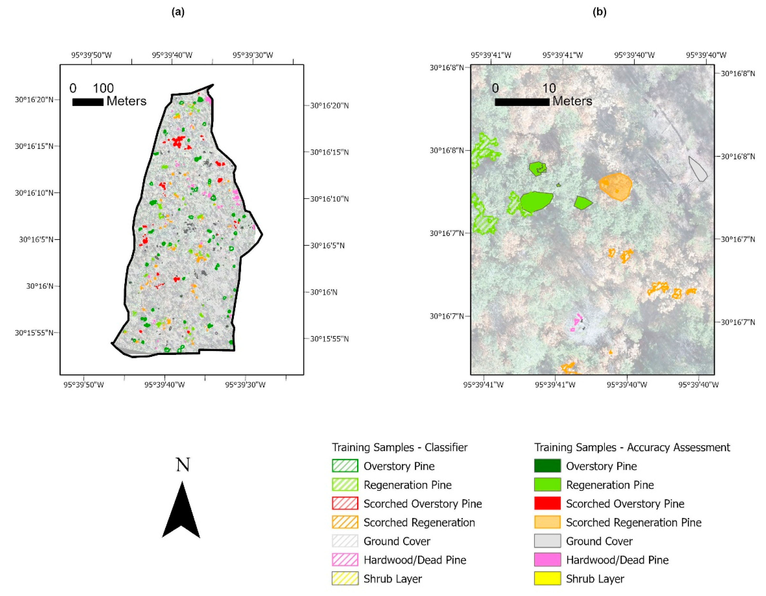
Overall, accuracy assessments yielded positive classification results amongst almost all the forest classes, but could be moderately to significantly impacted by the classifier used. Support Vector Machine produced the best accuracy results in ArcGIS Pro, and K-Nearest Neighbor in the case of eCognition. Support Vector Machine performed the worst when used in eCognition, and by a wide margin at 12% overall accuracy. While the Hardwood/Dead Pine class was not a target group for this study, classifiers performed relatively inaccurately when classifying this group.

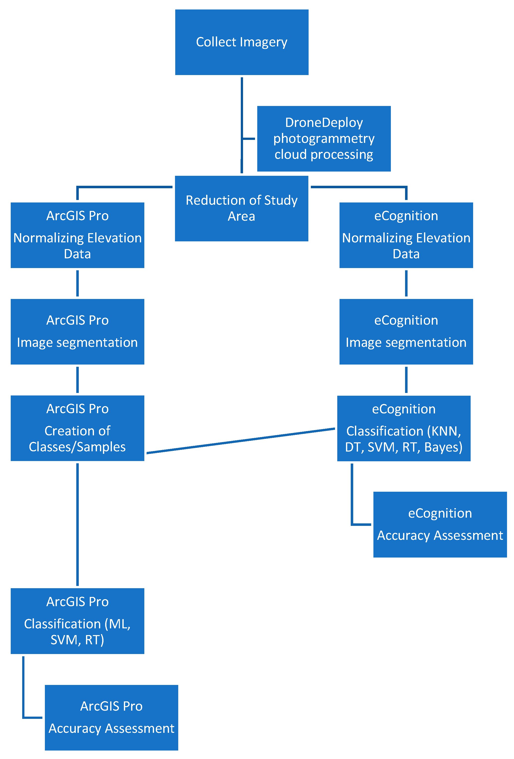
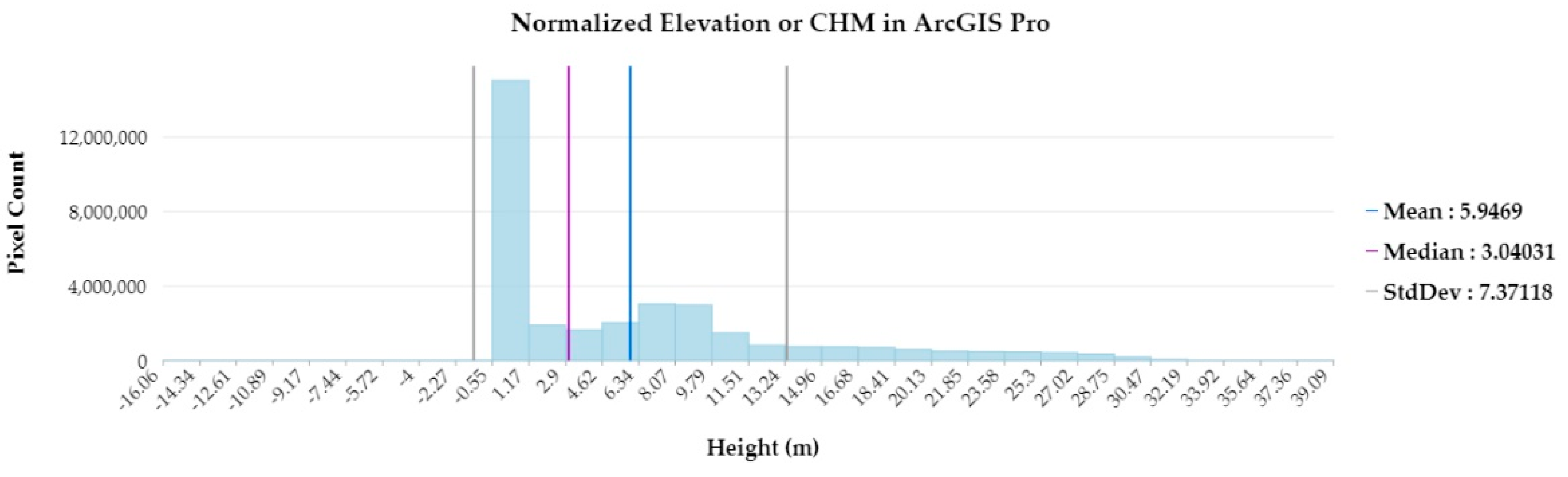
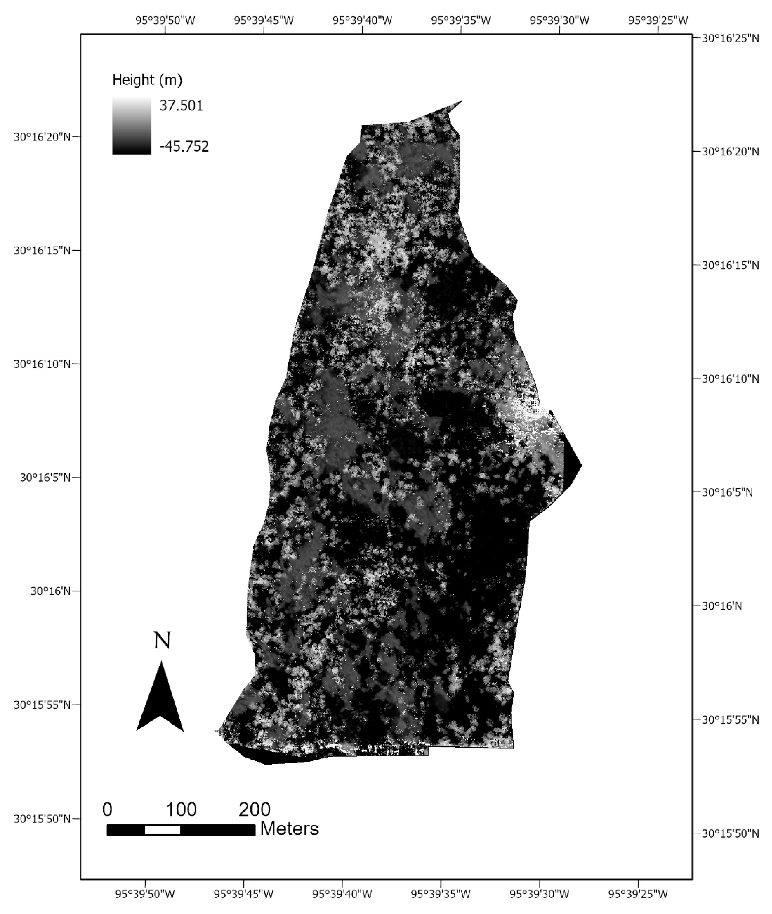
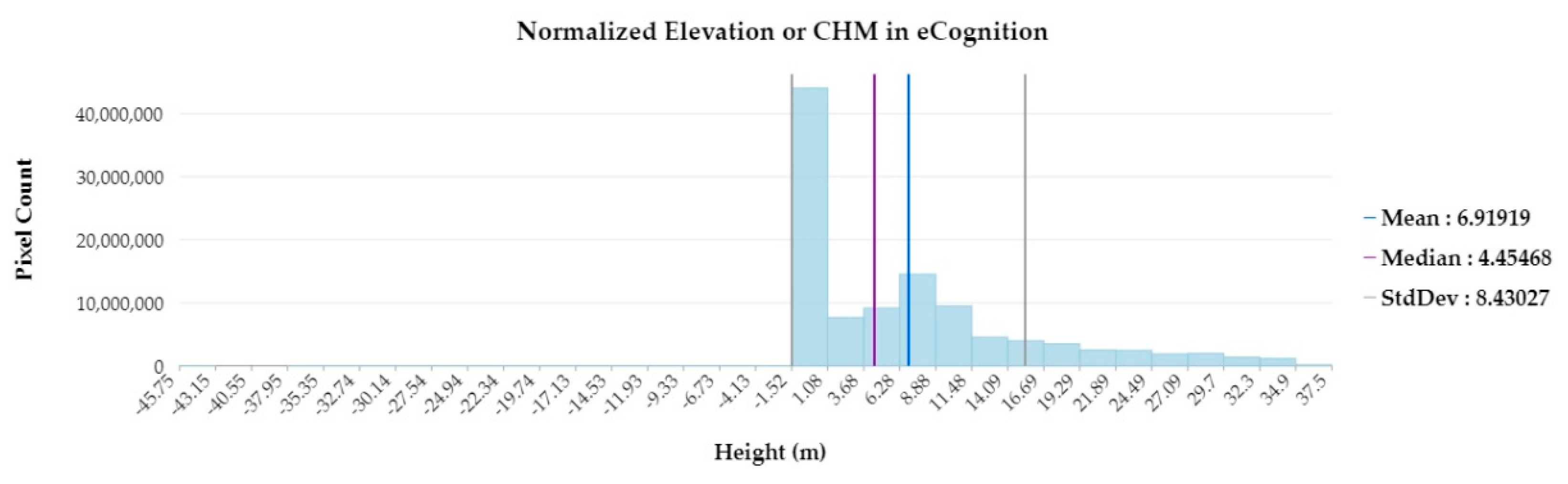
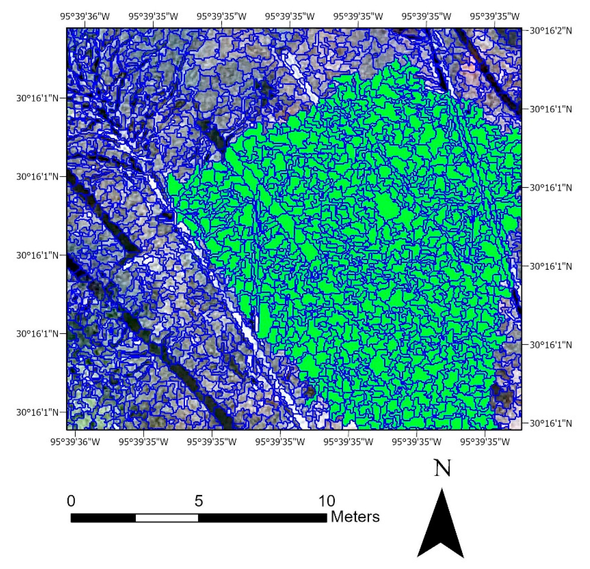
Reclassifying the CHM in ArcGIS Pro arguably had a positive impact on accuracy results and is possibly one explanation for its outperformance of eCognition. This extra step was the major difference between the two classification methodologies used in the software packages. Additionally, the image segmentation algorithms, and CHM outputs were slightly different for eCognition and ArcGIS Pro. Outside of these exceptions, both software programs used the same orthoimage, DTM, point cloud, training samples, and accuracy assessment samples.

Producer accuracy was consistently lower for overstory classes when compared to their regeneration counterparts. This is most likely because of the complex assortment of height classes found within an overstory pine’s canopy, and because fine resolution elevation data can penetrate past the upper-most canopy vegetation. Regeneration elevation data were typically more continuous, and not as interrupted by canopy openings large enough to create complex and variable elevation groupings. Therefore, training samples for regeneration classes were not capturing a variety of height classes, possibly resulting in higher producer accuracies. Random Trees in ArcGIS Pro was the most successful at reducing this error (

Table A2. Random Trees confusion matrix and classification results in ArcGIS Pro.

Class	Overstory	Regeneration	Overstory Scorched	Regeneration Scorched	Ground Cover	Deciduous/Dead Pine	Shrub Layer	Total
Overstory	51	1	15	0	0	1	0	68
Regeneration	5	48	0	2	0	0	0	55
Overstory Scorched	0	0	150	0	3	0	2	155
Regeneration Scorched	0	1	21	40	1	0	0	63
Ground Cover	3	0	12	0	83	1	1	100
Deciduous/Dead Pine	0	1	2	0	16	15	0	34
Shrub Layer	2	1	0	2	5	0	15	25
Total	61	52	200	44	108	17	18	500
Producer Accuracy	0.836066	0.923077	0.75	0.909090909	0.768519	0.882352941	0.833333
User Accuracy	0.75	0.872727273	0.967741935	0.634920635	0.83	0.441176471	0.6
Overall Accuracy	0.804
Kappa Index	0.751763

).

Low user accuracy for Hardwood/Dead Pine is consistent across all the ArcGIS Pro classifications, while producer accuracy is relatively high. This indicates that despite having well-referenced training samples, all three classification strategies struggled to accurately classify Hardwood/Dead Pine. A possible explanation is the spectral similarities between leaf-off hardwood and dead pine, and the frequent presence of dead, woody debris on the ground level. This creates a situation where objects of similar spectral characters, such as color and texture, also possess an unpredictable range of height classifications. Confusion matrix results appear to support this idea, with all three ArcGIS Pro classifiers possessing a significant amount of Ground Cover mistakenly classified as Hardwood/Dead Pine.

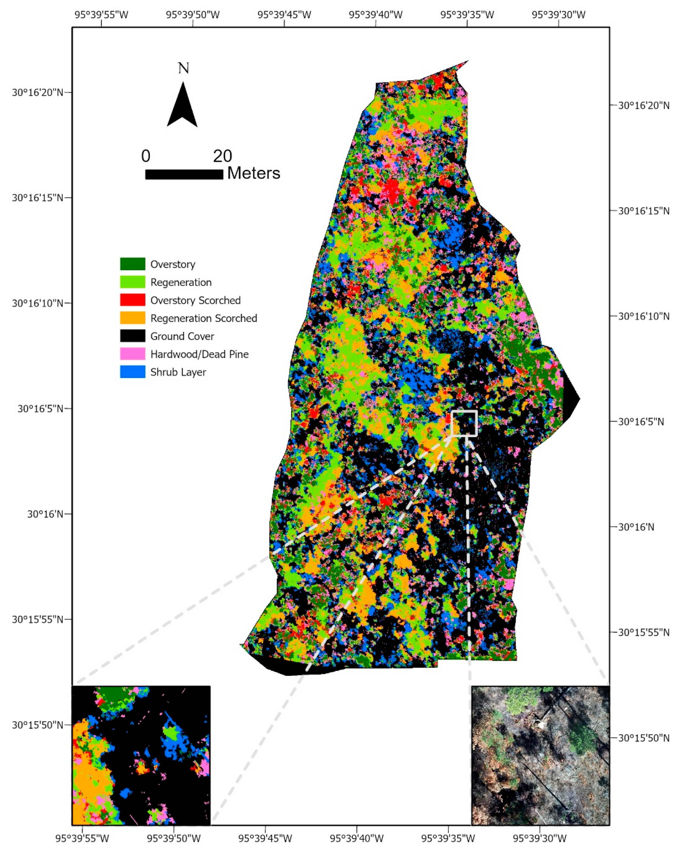
The results provide a number of insights into the quality of red-cockaded woodpecker habitat based on standards created by previous studies. The RCW recovery plan recommends managing for 40% or more herbaceous groundcover, with group size and reproduction increasing at this threshold [28]. Our measurement of Ground Cover was just shy of this threshold, at 38.09%. Next, a measure of woody hardwood with a height of approximately 2.7 m or less is made with our Shrub Layer class, at 7.01–15.24% depending on the classifier. A reduction in this class has shown to have a positive impact on RCW fitness, and here we successfully quantified and mapped its distribution. This information can help with vegetation management approaches such as mechanical removal or herbicidal treatments.

Comparisons can also be made between the amount of Pine Overstory to Pine Regeneration, and the ratio of Ground Cover to Shrub Layer. Both of these ratios are considered strong indicators of RCW habitat quality based on one study [33]. Specifically, the indicators used were the difference between 15–25 cm dbh trees and >35 cm dbh trees, and also the difference in groundcover between wiregrass and woody-plug-palmetto vegetation. Frances C. James et al. performed their work on the Wakulla and Apalachicola Ranger Districts in Florida, a region of Longleaf Pine RCW habitat far separated from our own study area. Despite the differences of study area, vegetation, etc., the habitat indicators are similar in many regards.

Quantifying and mapping the Pine Regeneration class was an important goal of this study. Pine regeneration is amongst the RCW habitat quality indicators, and of particular interests because of our goal of managing a long-term outlook when forest planning. Because Cook’s Branch Conservancy maintains an annual fire program to promote and improve RCW habitat, information about pine regeneration can help strategize where to burn and with what intensity. The seasonality of burning and particular burn conditions can help preserve or naturally thin pine regeneration, so this information informs forest managers of where to best apply fire.

Accurate and correctly reclassified elevation data were a key component of successful forest classification. For the sake of comparison, some iterations without elevation data were performed, along with unsupervised and pixel-based classification configurations. In all cases, classification accuracies were noticeably lower using the same training sample dataset. Most notably, the omission of elevation data resulted in significantly lower accuracy results, and so the inclusion of elevation data was not only necessary but confirmed the validity of Structure from Motion as a source of elevation data for our targeted classes.

A well-constructed training sample dataset was also important for accurate classification. This step, along with processing time during trial iterations, represent the most time-intensive portion of analysis. Once the parameters of a suitable training sample dataset were identified, they can be reproduced with much more efficiency in future and similar classification efforts.

The results of this study indicate the functionality of software applications, such as DroneDeploy, for creating elevation models using Structure from Motion photogrammetric methods, and how they can be leveraged in specific forest management scenarios. In this case, it effectively mapped indicators of RCW habitat quality. The time and cost efficiency are substantial when compared to hand-crew methods and highlight the value of continuing to further incorporate sUAS technologies into land management practices. Cost-savings are not only to the advantage of landowners, but to conservation efforts overall. sUAS gathered datasets will enable larger and more frequent coverage, along with potentially more detailed and accurate information on a comparable budget. Efforts to identify where data acquisition is most necessary, and how to effectively leverage it will likely be the challenge going forward.

References

1. Anderson, K.; Gaston, K. Lightweight unmanned aerial vehicles will revolutionize spatial ecology. Front. Ecol. Environ. 2013, 11, 138–146. [Google Scholar] [CrossRef] [Green Version]
2. Michez, A.; Piégay, H.; Lisein, J.; Claessens, H.; Lejeune, P. Discrimination of deciduous tree species from time series of unmanned aerial system imagery. PLoS ONE 2016, 10, e0141006. [Google Scholar] [CrossRef]
3. Hao, Z.; Lin, L.; Post, C.J.; Jiang, Y.; Li, M.; Wei, N.; Yu, K.; Liu, J. Assessing tree height and density of a young forest using a consumer unmanned aerial vehicle (UAV). New For. 2021, 52, 843–862. [Google Scholar] [CrossRef]
4. Devriendt, L.; Bonne, J. UAS mapping as an alternative for land surveying techniques? Int. Arch. Photogramm. Remote Sens. Spat. Inf. Sci. 2014, 40, 39. [Google Scholar] [CrossRef] [Green Version]
5. Šedina, J.; Pavelka, K.; Raeva, P. UAV Remote Sensing Capability for Precision Agriculture, Forestry and Small Natural Reservation Monitoring; Bannon, D.P., Ed.; International Society for Optics and Photonics: Anaheim, CA, USA, 2017; p. 102130L. [Google Scholar] [CrossRef]
6. Ramalho de Oliveira, L.F.; Lassiter, H.A.; Wilkinson, B.; Whitley, T.; Ifju, P.; Logan, S.R.; Peter, G.F.; Vogel, J.G.; Martin, T.A. Moving to automated tree inventory: Comparison of UAS-derived Lidar and photogrammetric data with manual ground estimates. Remote Sens. 2020, 13, 72. [Google Scholar] [CrossRef]
7. Mishra, P.K.; Rai, A. Role of unmanned aerial systems for natural resource management. J. Indian Soc. Remote Sens. 2021, 49, 671–679. [Google Scholar] [CrossRef]
8. Watts, A.C.; Ambrosia, V.G.; Hinkley, E.A. Unmanned aircraft systems in remote sensing and scientific research: Classification and considerations of use. Remote Sens. 2012, 4, 1671–1692. [Google Scholar] [CrossRef] [Green Version]
9. Agrawal, A.; Chhatre, A.; Hardin, R. Changing governance of the world’s forests. Science 2008, 320, 1460–1462. [Google Scholar] [CrossRef]
10. Colfer Pierce, J.C.; Dahal Ram, G.; Capistrano, D. Lessons from Forest Decentralization: Money, Justice and the Quest for Good Governance in Asia-Pacific; Taylor and Francis: Hoboken, NJ, USA, 2012. [Google Scholar]
11. Agrawal, A.; Chhatre, A. Explaining success on the commons: Community forest governance in the Indian Himalaya. World Dev. 2006, 34, 149–166. [Google Scholar] [CrossRef]
12. Mcconnell, W.J.; Sweeney, S.P. Challenges of forest governance in Madagascar. Geogr. J. 2005, 171, 223–238. [Google Scholar] [CrossRef]
13. Delabre, I.; Boyd, E.; Brockhaus, M.; Carton, W.; Krause, T.; Newell, P.; Wong, G.Y.; Zelli, F. Unearthing the myths of global sustainable forest governance. Glob. Sustain. 2020, 3, e16. [Google Scholar] [CrossRef]
14. Kuusela, A. Drones as Information System Artifacts Supporting Environmental Sustainability in Finnish Forest Industry; University of Jyväskylä: Jyväskylä, Finland, 2020. [Google Scholar]
15. Paneque-Gálvez, J.; McCall, M.; Napoletano, B.; Wich, S.; Koh, L. Small drones for community-based forest monitoring: An assessment of their feasibility and potential in tropical areas. Forests 2014, 5, 1481–1507. [Google Scholar] [CrossRef] [Green Version]
16. Portillo-Quintero, C.; Hernández-Stefanoni, J.L.; Reyes-Palomeque, G.; Subedi, M.R. The road to operationalization of effective tropical forest monitoring systems. Remote Sens. 2021, 13, 1370. [Google Scholar] [CrossRef]
17. Sjaf, S. Mapping the village forest of Pattaneteang through drone participatory mapping. IOP Conf. Ser. Earth Environ. Sci. 2021, 879, 012028. [Google Scholar] [CrossRef]
18. Swinfield, T.; Lindsell, J.A.; Williams, J.V.; Harrison, R.D.; Habibi, A.; Gemita, E.; Schönlieb, C.B.; Coomes, D.A. Accurate measurement of tropical forest canopy heights and aboveground carbon using structure from motion. Remote Sens. 2019, 11, 928. [Google Scholar] [CrossRef] [Green Version]
19. Wallace, L.; Lucieer, A.; Malenovský, Z.; Turner, D.; Vopěnka, P. Assessment of forest structure using two UAV techniques: A comparison of airborne laser scanning and structure from motion (SfM) point clouds. Forests 2016, 7, 62. [Google Scholar] [CrossRef] [Green Version]
20. Lisein, J.; Pierrot-Deseilligny, M.; Bonnet, S.; Lejeune, P. A photogrammetric workflow for the creation of a forest canopy height model from small unmanned aerial system imagery. Forests 2013, 4, 922–944. [Google Scholar] [CrossRef] [Green Version]
21. Iglhaut, J.; Cabo, C.; Puliti, S.; Piermattei, L.; O’Connor, J.; Rosette, J. Structure from motion photogrammetry in forestry: A review. Curr. For. Rep. 2019, 5, 155–168. [Google Scholar] [CrossRef] [Green Version]
22. Zhou, X.; Zhang, X. Individual tree parameters estimation for plantation forests based on UAV oblique photography. IEEE Access 2020, 8, 96184–96198. [Google Scholar] [CrossRef]
23. Zhang, H.; Bauters, M.; Boeckx, P.; Van Oost, K. Mapping canopy heights in dense tropical forests using low-cost UAV-derived photogrammetric point clouds and machine learning approaches. Remote Sens. 2021, 13, 3777. [Google Scholar] [CrossRef]
24. Mohan, M.; Leite, R.V.; Broadbent, E.N.; Wan Mohd Jaafar, W.S.; Srinivasan, S.; Bajaj, S.; Dalla Corte, A.P.; do Amaral, C.H.; Gopan, G.; Saad, S.N.M.; et al. Individual tree detection using UAV-Lidar and UAV-SfM data: A tutorial for beginners. Open Geosci. 2021, 13, 1028–1039. [Google Scholar] [CrossRef]
25. Windrim, L.; Carnegie, A.J.; Webster, M.; Bryson, M. Tree detection and health monitoring in multispectral aerial imagery and photogrammetric pointclouds using machine learning. IEEE J. Sel. Top. Appl. Earth Obs. Remote Sens. 2020, 13, 2554–2572. [Google Scholar] [CrossRef]
26. Michez, A.; Piégay, H.; Jonathan, L.; Claessens, H.; Lejeune, P. Mapping of riparian invasive species with supervised classification of unmanned aerial system (UAS) imagery. Int. J. Appl. Earth Obs. Geoinf. 2016, 44, 88–94. [Google Scholar] [CrossRef]
27. Bendig, J.; Bolten, A.; Bennertz, S.; Broscheit, J.; Eichfuss, S.; Bareth, G. Estimating biomass of barley using crop surface models (CSMs) derived from UAV-based RGB imaging. Remote Sens. 2014, 6, 10395–10412. [Google Scholar] [CrossRef] [Green Version]
28. U.S. Fish and Wildlife Service. Recovery Plan for the Red-Cockaded Woodpecker (Picoides borealis): Second Revision; U.S. Fish and Wildlife Service: Atlanta, GA, USA, 2003; p. 296.
29. Rudolph, C.D.; Connor, R.N. Cavity tree selection by red-cockaded woodpeckers in relation to tree age. Wilson Bull. 1991, 103, 458–467. [Google Scholar]
30. Conner, R.; Rudolph, D.C.; Walters, J.R. The Red-Cockaded Woodpecker: Surviving in a Fire-Maintained Ecosystem; University of Texas Press: Austin, TX, USA, 2001; Volume 49. [Google Scholar]
31. Hovis, J.A.; Labisky, R.F. Vegetative associations of red-cockaded woodpecker colonies in Florida. Wildl. Soc. Bull. 1985, 13, 307–314. [Google Scholar]
32. Walters, J.R.; Daniels, S.J.; Carter, J.H.; Doerr, P.D. Defining quality of red-cockaded woodpecker foraging habitat based on habitat use and fitness. J. Wildl. Manag. 2002, 66, 1064. [Google Scholar] [CrossRef]
33. James, F.C.; Hess, C.A.; Kicklighter, B.C.; Thum, R.A. Ecosystem management and the niche gestalt of the red-cockaded woodpecker in longleaf pine forests. Ecol. Appl. 2001, 11, 854–870. [Google Scholar] [CrossRef]
34. James, F.C.; Hess, C.A.; Kufrin, D. Species-centered environmental analysis: Indirect effects of fire history on red-cockaded woodpeckers. Ecol. Appl. 1997, 7, 118–129. [Google Scholar] [CrossRef]
35. Smart, L.S.; Swenson, J.J.; Christensen, N.L.; Sexton, J.O. Three-dimensional characterization of pine forest type and red-cockaded woodpecker habitat by small-footprint, discrete-return Lidar. For. Ecol. Manag. 2012, 281, 100–110. [Google Scholar] [CrossRef]
36. Dean, T.J.; Cao, Q.V.; Roberts, S.D.; Evans, D.L. Measuring heights to crown base and crown median with Lidar in a mature, even-aged loblolly pine stand. For. Ecol. Manag. 2009, 257, 126–133. [Google Scholar] [CrossRef]
37. Van Rees, E. Creating aerial drone maps fast. GEOInformatics 2015, 18, 24–25. [Google Scholar]
38. Kameyama, S.; Sugiura, K. Effects of differences in structure from motion software on image processing of unmanned aerial vehicle photography and estimation of crown area and tree height in forests. Remote Sens. 2021, 13, 626. [Google Scholar] [CrossRef]
39. Xie, Z.; Chen, Y.; Lu, D.; Li, G.; Chen, E. Classification of land cover, forest, and tree species classes with ZiYuan-3 multispectral and stereo data. Remote Sens. 2019, 11, 164. [Google Scholar] [CrossRef] [Green Version]
40. Qian, Y.; Zhou, W.; Yan, J.; Li, W.; Han, L. Comparing machine learning classifiers for object-based land cover classification using very high resolution imagery. Remote Sens. 2014, 7, 153–168. [Google Scholar] [CrossRef]
41. Millard, K.; Richardson, M. On the importance of training data sample selection in random forest image classification: A case study in peatland ecosystem mapping. Remote Sens. 2015, 7, 8489–8515. [Google Scholar] [CrossRef] [Green Version]
42. Kattenborn, T.; Eichel, J.; Fassnacht, F.E. Convolutional neural networks enable efficient, accurate and fine-grained segmentation of plant species and communities from high-resolution UAV imagery. Sci. Rep. 2019, 9, 17656. [Google Scholar] [CrossRef]
43. Sabat-Tomala, A.; Raczko, E.; Zagajewski, B. Comparison of support vector machine and random forest algorithms for invasive and expansive species classification using airborne hyperspectral data. Remote Sens. 2020, 12, 516. [Google Scholar] [CrossRef] [Green Version]
44. Flora of North America Editorial Committee. Flora of North America North of Mexico; Oxford University Press: Oxford, UK; New York, NY, USA, 1993; Volume 22, Available online: http://beta.floranorthamerica.org (accessed on 7 January 2022).
Figure 1. A summarized workflow of this study.
Drones 06 00026 g001
Figure 2. Flight path transects, image capture points, and GPS quality during sUAS flights. The color gradient provides a reference for coverage quality found in the study area. Additionally, unaligned, or only GPS aligned capture points are symbolized, and correlate with poor coverage quality in some cases.
Drones 06 00026 g002
Figure 3. The orthoimage created by DroneDeploy after processing, including a smaller-scale image of the detail acquired.
Drones 06 00026 g003
Figure 4. The DTM created by DroneDeploy after processing.
Drones 06 00026 g004
Figure 5. The point cloud created by DroneDeploy in 2-D (top) and 3-D (bottom) views.
Drones 06 00026 g005
Figure 6. A Canopy Height Model produced after normalizing elevation values from the rasterized point cloud. Negative, aberrant elevation values are found in the western half where GPS alignment issues occurred. This area was excluded, and a reduced study area is delineated in white. The selected area was captured during one continuous sUAS flight.
Drones 06 00026 g006
Figure 7. Histogram of the CHM values produced in ArcGIS Pro. The average height was approximately 6 m, and median height was approximately 3 m.
Drones 06 00026 g007
Figure 8. The study area’s orthoimage (a) alongside its corresponding height reclassification (b). The orthoimage and CHM were used together to identify where major height classes are occurring. Examples of height classes after reclassifying the CHM are labeled: (1) represents ground cover, (2) shrub layer, (3) a pine overstory canopy, and (4) is an area of scorched regeneration.
Drones 06 00026 g008
Figure 9. An area of pine regeneration, both scorched and unscorched. The orthoimage (a) is seen on the right, and the classified elevation (b) on the left. These areas typically were tallest in central portions and consist of level 1–3 midstory elevations.
Drones 06 00026 g009
Figure 10. A map of the CHM once it was reclassified into height classes that represent the major forest characters.
Drones 06 00026 g010
Figure 11. The orthoimage on the left and segmented image on the right demonstrate what segmentation looks like.
Drones 06 00026 g011
Figure 12. The image on the left (a) illustrates the entire distribution of training samples used for training classifiers and accuracy assessment. The right image (b) shows a larger scale example of training samples in a regeneration area.
Drones 06 00026 g012
Figure 13. A filtered CHM used for image segmentation in eCognition. While the heights range as low as approximately 45 m, a negligible amount of the values are negative, as seen on the histogram for the eCognition (Figure 14).
Drones 06 00026 g013
Figure 14. Histogram of the CHM values produced in eCognition. The average height was approximately 7 m, and median height was approximately 4.5 m.
Drones 06 00026 g014
Figure 15. An illustration of what image objects looked like post-segmentation, and an example of image objects that were captured by the thematic layer and generated into training samples.
Drones 06 00026 g015
Figure 16. SVM classification map produced in ArcGIS Pro. The bottom left displays a larger-scale image of the classification output, and the bottom left is the corresponding orthoimage.
Drones 06 00026 g016
Figure 17. KNN classification map produced in eCognition. The bottom left displays a larger-scale image of the classification output, and the bottom left is the corresponding orthoimage.
Drones 06 00026 g017