1. Introduction
Air-to-surface missions (ASMs) are becoming increasingly dangerous in modern warfare, where the successful performance of ASMs is strategically important. To deal with this issue, missions are carried out using stealth aircraft to avoid threats on recent battlefields. However, developing an aircraft with stealth capabilities is costly and does not exclude threats to pilots’ lives altogether. Performing ASMs using Unmanned Combat Aerial Vehicles (UCAVs) is an effective approach to handling these difficulties. For this reason, many studies have been conducted to perform missions using UCAVs. Through these efforts, several approaches are proposed to efficiently plan ASMs [
1,
2,
3,
4,
5,
6,
7,
8,
9,
10,
11,
12,
13,
14] in
Table 1. Randal W Beard et al. [
1] proposed an ASM planning algorithm for multiple UCAVs. The proposed algorithm plans the path based on the Voronoi-diagram concept and assigns the targets to UCAVs to minimize the prescribed objective function. Path planning based on the Voronoi diagram concept is advantageous for planning a path, which bypasses threats to the maximum extent. However, with the cost of creating unnecessary detours. Yeonju Eun et al. [
2] proposed a path planner which combines the Voronoi-diagram concept and potential field concept to address this issue for Suppression to Enemy Air Defenses(SEAD) mission planning. There is a limitation that these algorithms are only applied to two-dimensional environments. H.H Triharminto et al. [
3], proposed a path planner for moving target intercept on dynamic 3D environments, but the algorithm focuses only on local environments. Meanwhile, several path planners using Dubins path concept for target intercept were proposed [
4,
5,
6]. These approaches have the advantage of being able to consider the dynamic constraints of aircraft and simply generate an optimal path. However, it has not been verified in a three-dimensional environment. Most of the proposed studies focus on generating paths to approach targets in a 2D global environment or generate only a path to pursue and intercept a target in a 3D environment. To contribute to this issue, an ASM planning technique that can simultaneously plan the path to approach the targets and the path to hit the targets while considering both threats and obstacles in the 3D environment is addressed in this paper.
ASMs are classified into several detailed missions, depending on the mission’s environment and goals as follows: Air Interdiction (AI), Close Air Support (CAS), Suppression to Enemy Air Defenses (SEAD), and Attack Operations (AO). According to the U.S. Air Force Doctrine [
15,
16], AO and SEAD missions fall under the category of Offensive Counterair(OCA) missions, while AI and CAS missions belong to the category of counterland missions. AO is intended to destroy, disrupt, or degrade counterair targets including enemy air and missile threats, their command and control, and their support infrastructure on the ground such as airfields, launch sites, launchers, fuel, supplies, etc. The SEAD missions aim to neutralize, destroy, or degrade enemy surface-based air defenses by destructive or disruptive means. While AO focuses on preventive measures to strike the enemy air defense assets before they are deployed, there is a difference that the SEAD mission aims to neutralize the already deployed enemy air defense assets. On the other hand, the AI missions’ goal is to preemptively disrupt, delay, or destroy the enemy’s military potential before it responds effectively to friendly forces. Whereas the CAS mission aims to strike against hostile targets that are near close to friendly forces. Since the enemy targets are near friendly forces, tracking of friendly forces’ movements and careful firing on targets are more crucial than in the case of the AI missions. However, since the targets of AI missions are usually within enemy territory, the number of interspersed threats within the mission environment is likely to be greater than that of CAS missions.
These ASMs have in common that they basically perform consecutive mission elements of ingress, intercept, and egress. The ingress mission element is the phase of approaching the intercept mission area while avoiding the various threats that appear when entering a hostile area. Then, the aircraft intercepts the target quickly and accurately in the intercept mission element. Lastly, the egress mission element is the phase of escaping the hostile area while avoiding scattered threats. Since the ASM planner can be designed through a strategy of sequential planning on each mission element. For ingress and egress missions, avoiding enemy radar detection and air defense threats are foremost important. Stealth aircraft may be a solution, but detection avoidance through low-fly flight maneuvers which is called hedgehop can also be a good approach. Therefore, a terrain flight path planner is proposed to generate a contour chasing flight path for the ingress and egress mission element maneuver path planning. In the intercept phase, it is important to strike the target as quickly as possible rather than avoiding the threats. Thus, an algorithm is proposed that can generate the shortest target intercept path in this paper.
The paper is structured as follows. In
Section 2, terrain and threat modeling techniques are treated to describe the real-world battlefield environments. Terrain flight path planner based on RRT* algorithm that can generate asymptotic global optimal path is addressed in
Section 3. The shortest target intercept path planner is addressed in
Section 4. In
Section 5, several test scenarios are presented for the validation of the presented mission planner. In
Section 6, The integrated mission planner is validated through applications on the proposed scenarios. Furthermore, simulations are performed using a rotorcraft model to track the generated trajectories.
Section 7 provides the important details and analysis of the results are summarized in the conclusion.
2. Mission Environment Construction
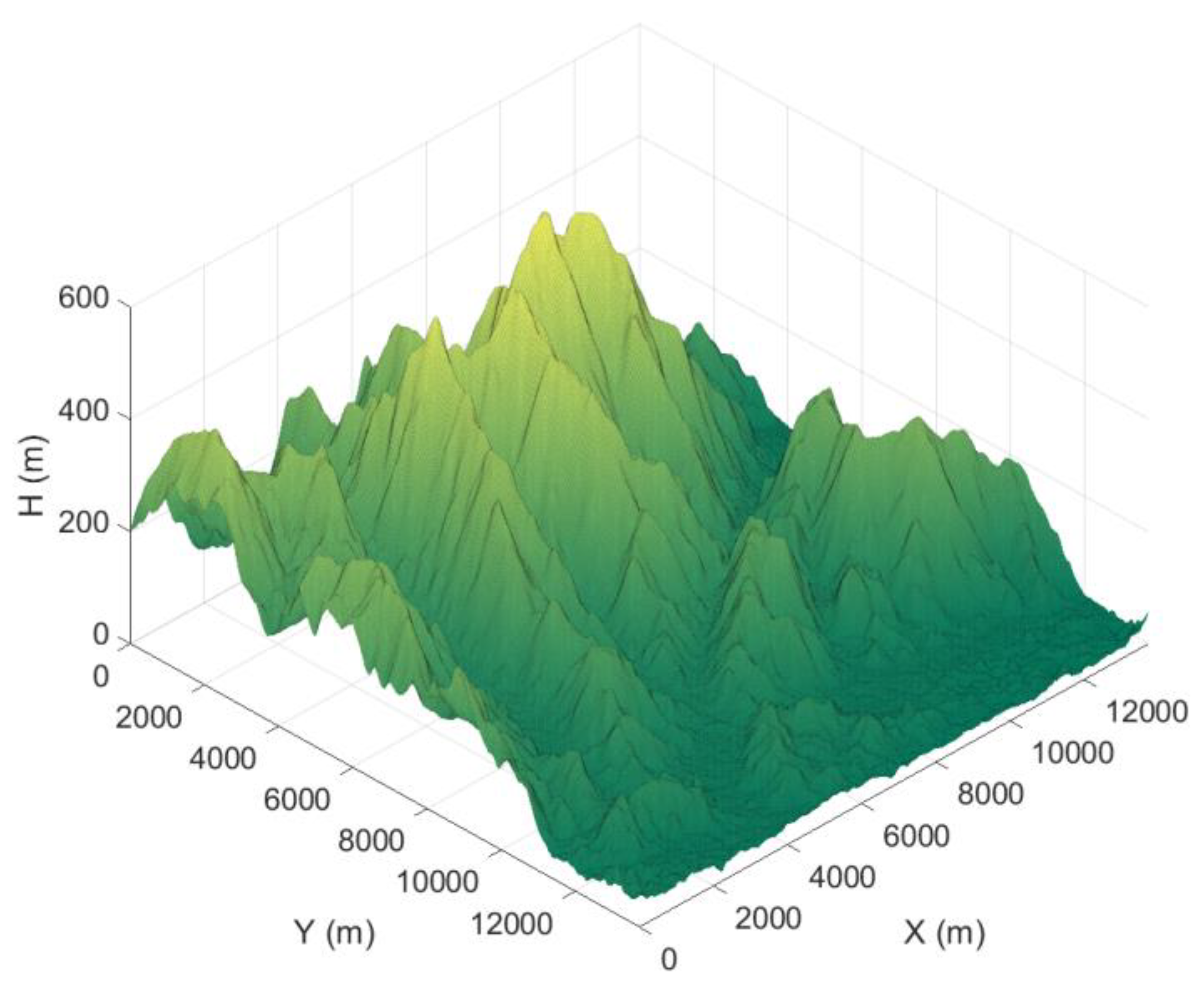
Building a virtual mission environment is crucial when designing path planning algorithms for ASMs. Therefore, this section treats the techniques used to increase the applicability of the designed path planner when building the real battlefield environment including terrain threat models. The terrain height model of the real world is inserted into the planning environment to describe actual battlefields such as in
Figure 1. The maximum height of the terrain is 591 m while both the X-axis and Y-axis are 13,745.58 m wide. The terrain map was generated based on the terrain heightmap near 37°25′20.2” N, 127°01′21.9” E.
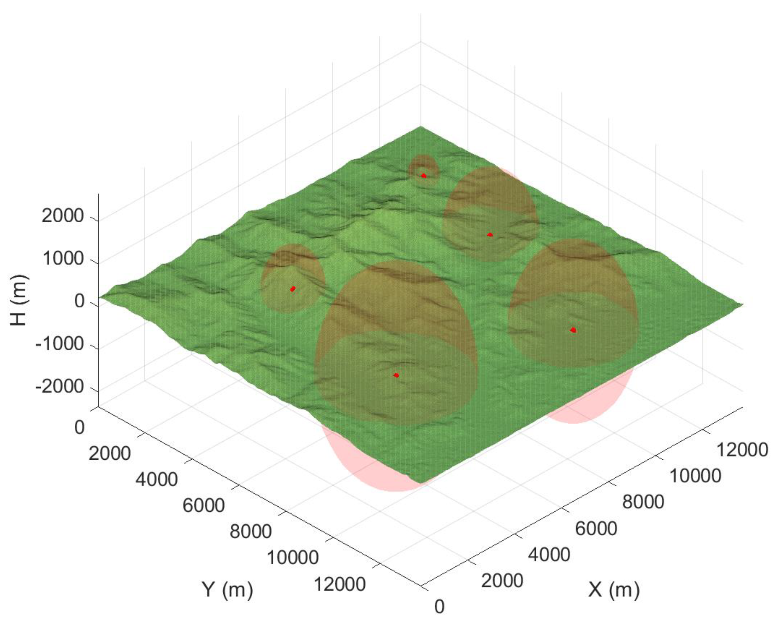
In addition, a spherical threat model is proposed which has a radius of maximum threat reach and Radial Basis Function (RBF) based threat strength distribution in the inner domain of the sphere to describe common threat types. Equation (1) shows the threat strength distribution in the inner domain of the threat:
where
represents the position vector of a node, and
represents the position vector of a threat. The strength of the threat center is
, and the proportion of the threat varies according to the distance from the center of the threat and the RBF shape factor
. Furthermore, the threat disappears when it is outside of the maximum threat distance. In this paper, the Gaussian function shown in Equation (2) is selected as the threat distribution [
17]. Other types of RBF can also be adopted depending on the mission environment.
Figure 2 represents an example of a terrain map with five threat models.
3. Terrain Flight Path Planner
UCAVs must avoid multiple threats in the hostile area to perform ingress and egress mission elements. Therefore, there is a need for a Terrain Flightpath planner which is capable of avoiding threats while avoiding detection of enemy radar through a low approach. There are a number of path planning algorithms that can be applied to this problem. Path Planning algorithms are commonly classified into five different categories [
18]: sampling-based algorithms, node-based algorithms, mathematic model-based algorithms, bio-inspired algorithms, and multifusion-based algorithms. Among them, the sampling-based algorithm can be used in both static and dynamic environments, with high time efficiency. The Rapidly-exploring Random Tree (RRT) algorithm [
19] is one of the active sampling-based algorithms which is well-known for its fast convergence in multidimensional environments. However, the RRT algorithm has the shortcoming that it cannot guarantee an optimal path. To overcome this shortcoming, the RRT* algorithm [
20] has been proposed. In the RRT* algorithm, an asymptotic optimal path can be reached through sufficient iterations by adding a routine to update the tree considering the path cost. However, its slow convergence rate became another issue. The RRT*-smart [
21] algorithm was proposed to improve this weakness by accelerating the convergence rate to the asymptotic optimal path using intelligent sampling. In addition, the P-RRT* [
22] algorithm with a potential-guided sampling technique was proposed to increase the convergence rate for the initial path. There are many other recent approaches to improve performance and overcome shortcomings of the RRT-based algorithms [
23,
24,
25,
26,
27,
28]. However, analyzing and applying all these algorithms requires a high excessive workload. Therefore, the P-RRT*-smart algorithm is selected and applied which is a fusion of classical P-RRT* and RRT*-smart to cover the applicability of a wide range of the path planning algorithms.
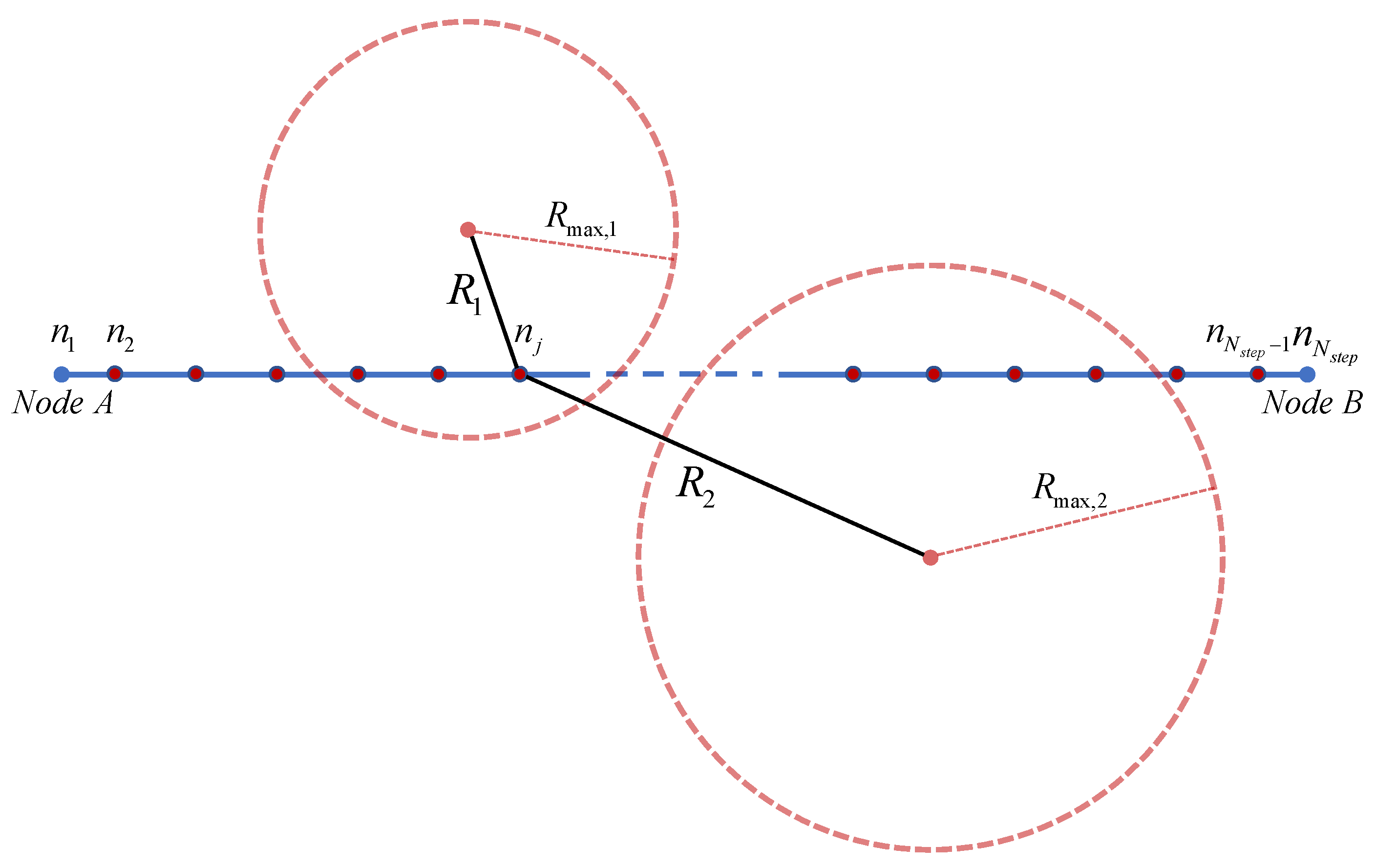
The following additional approaches are also applied when planning the terrain flight path. Areas over a certain distance from the surface are treated as obstacles. To do so, the generated path is always located near the surface. In addition, the cost due to threats between two nodes
is calculated as follows:
where
is the total number of threats in the environment and
is the total number of steps between two nodes. In Equation (3), the step cost
in each step is calculated using the cost function presented in Equation (1) while advancing between nodes by the prescribed step size. By summing all the calculated step costs, the cost due to threats between the nodes can be calculated. Since the cost due to threats continues to add up while the aircraft is within the threat range (i.e.,
), it is possible to account for the cost change depending on the flight time consumed within the threat range. A geometrical schematic of the step cost concept at an arbitrary j-th step between two nodes in the presence of two existing threats is shown in
Figure 3.
The node-to-node cost
can then be calculated by additionally considering the distance cost between nodes as:
where
and
are the position vectors of nodes A and B, respectively.
Figure 4 represents an example case of terrain path planning. The path planning and all the other simulations are performed by Visual Fortran, Window 10 home, with the help of Intel Core i7-6700K CPU (4.0 GHz) with 32 GB of RAM. The total running time is 2.251 s with the 5000 total number of samplings. However, both the initial path convergence and the optimal path convergence times are quite short, 0.096 s and 0.7344 s, respectively. As shown in
Figure 4a, the planned path avoids a threat with relatively strong strength to minimize the path cost. In addition, the planned path is generated within 100 m of the vertical distance from the surface as shown in
Figure 5.
4. Shortest Target Intercept Path Planner
The target areas are likely to be interspersed with threats that take hostile actions. To increase the chances of completing a successful mission, the aircraft must survive during the intercept process. Accordingly, it is necessary to generate the shortest distance path from the vicinity of the target area so that the mission can be carried out as quickly as possible. Furthermore, in order to attack the target point, the aircraft’s heading angle should be aligned with the target point before the action takes place. Considering two necessary conditions, the Dubins circle can provide reliable results. Dubins [
29] presented a method to generate the shortest path to reach the final position and heading while satisfying the constraint that vehicles must move along the arcs of a minimal turning radius
while proceeding in the initially prescribed heading. The path generated by this approach may not be an obstacle-free path, and therefore can only be used in an environment undisturbed by obstacles. However, this approach is useful since it can generate a simple and fast flyable path. Based on this advantage, a planner was designed to plan the path of the target intercept mission element.
The concept of a target intercept path planning strategy is shown in
Figure 6. First, the position and entry angle of the target and position and heading angle of the UCAV is prescribed. Furthermore, the height of the intercept mission plane is set to an XY plane high enough from the highest terrain height in the intercept mission area. The UCAV aims at the target while flying straight in the direction of the given entry angle
. Thus, the aiming start position and weapon release point are defined as points separated by certain distances
and
in the direction of the entry angle from the target. Next, the path is generated by connecting the initial position of the UCAV, the aiming start position, and the weapon release point based on the Dubins path concept [
30]. The same process is repeated until the path is generated which intercepts all the targets. Finally, the rest of the path is generated with the prescribed exit point and exit angle from the last target location. In this concept,
can be determined by the aircraft’s dynamic characteristics and speed, and
,
can be determined by the missile’s aiming capability.
The length of the path generated by the presented process varies according to the intercept entry angles and the target intercept sequence. Therefore, the entry angles are needed to be optimized to obtain the shortest path. The optimization problem can be formulated as Equation (5). The object function
is the total length of the generated path and the design variables
are the intercept entry angles of each target. The formulated problem can be solved using an NLP solver and the robust SQP method [
31] is applied in this paper.
However, the target intercept sequence is another factor that determines the length of the path. Accordingly, the target intercept sequence in which the path length is minimized should be determined. Therefore, optimization is performed on all possible combinations of target intercept sequences, and a combination having the shortest path length is selected.
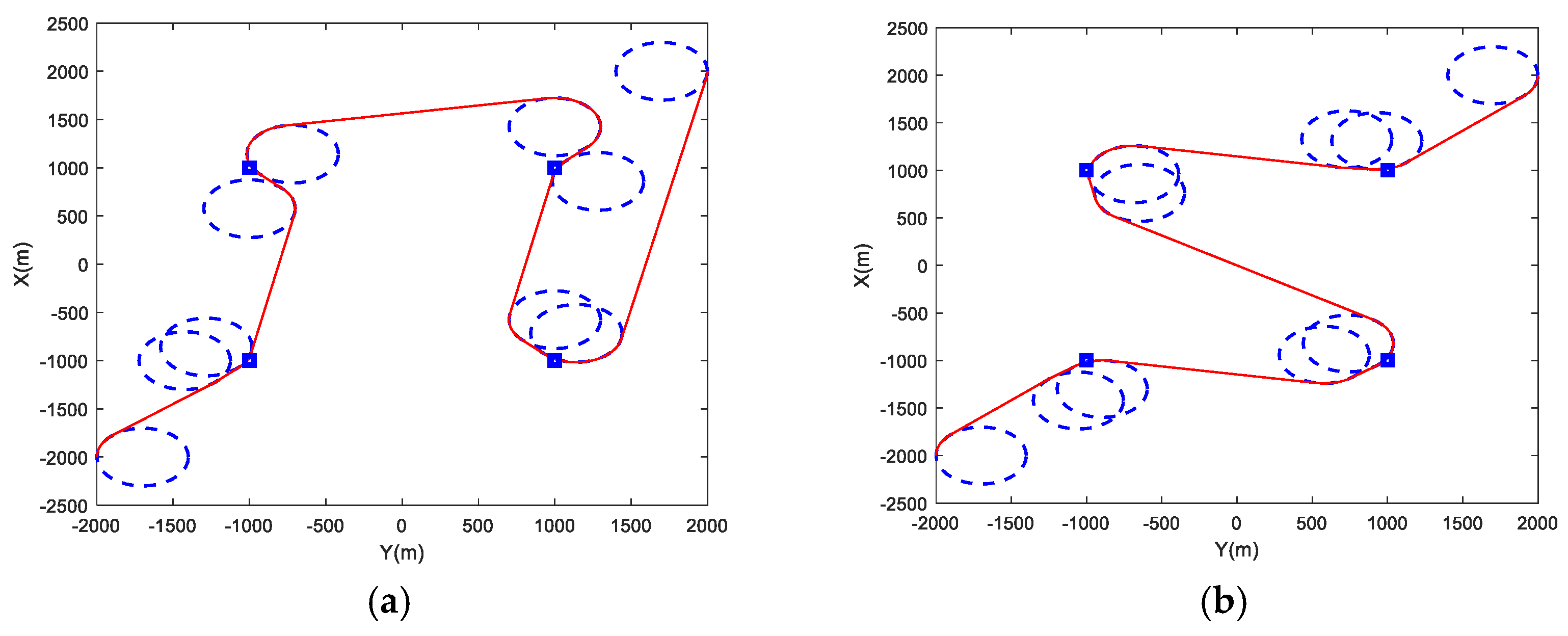
Figure 7 illustrates an example case of the proposed planner. The square points represent the location of the targets. Furthermore, each of the parameters
,
, and
were set to 300 m, 100 m, and 300 m, respectively. The solid line represents the planned path, and the dash lines describe the turning radius. The total consumed time to optimizing was 3.524 s.
Figure 7 shows that the target entry angles, and target intercept sequence are properly optimized.
The computation time seems unsuitable for real-time computation. However, this time is the time it takes when optimization is performed with the initial value set to 0 for all possible intercept sequences. When in flight, a strategy of updating the path in real-time can be taken while setting the initial value to the previously optimized value and performing optimization for a single intercept sequence. To validate this strategy, optimization was performed by changing each target position shown in
Figure 7 by 100 m, setting the previously optimized entry angles to the initial values, and performed for the previously optimized intercept sequence. The time required for optimization was 0.2190 s, confirming the possibility of real-time application.
5. Application on Mission Scenarios
ASMs consist of AI, CAS, SEAD, and AO missions depending on the mission environment and its goal. The major differences between these four missions are the density and distribution of threats on the environment and the property of the targets.
First, in the environmental perspective view, AI and AO missions require the UCAVs to penetrate deep into the enemy territory. Therefore, there is a possibility of many scattered threats along UCAVs’ path. In SEAD missions, most targets are located on highlands since air defense assets are already deployed. CAS missions generally aim to strike targets located on the border between enemy and friendly territories where the number of threats increases when approaching the target intercept area.
Second, in the target property perspective view, all hostile assets can be targeted in counterland missions, including the enemy’s military potential, whereas only enemy air defense assets are targeted in counterair missions. However, there is no difference when planning the path of the two missions since there is a commonality that the targets are located on the surface. For this reason, the proposed planner validation for AI, AO, and CAS missions can be performed together in a single mission scenario. Considering that the targets of the SEAD mission are located on the highlands, another mission scenario is also constructed.
5.1. AI Mission Scenario
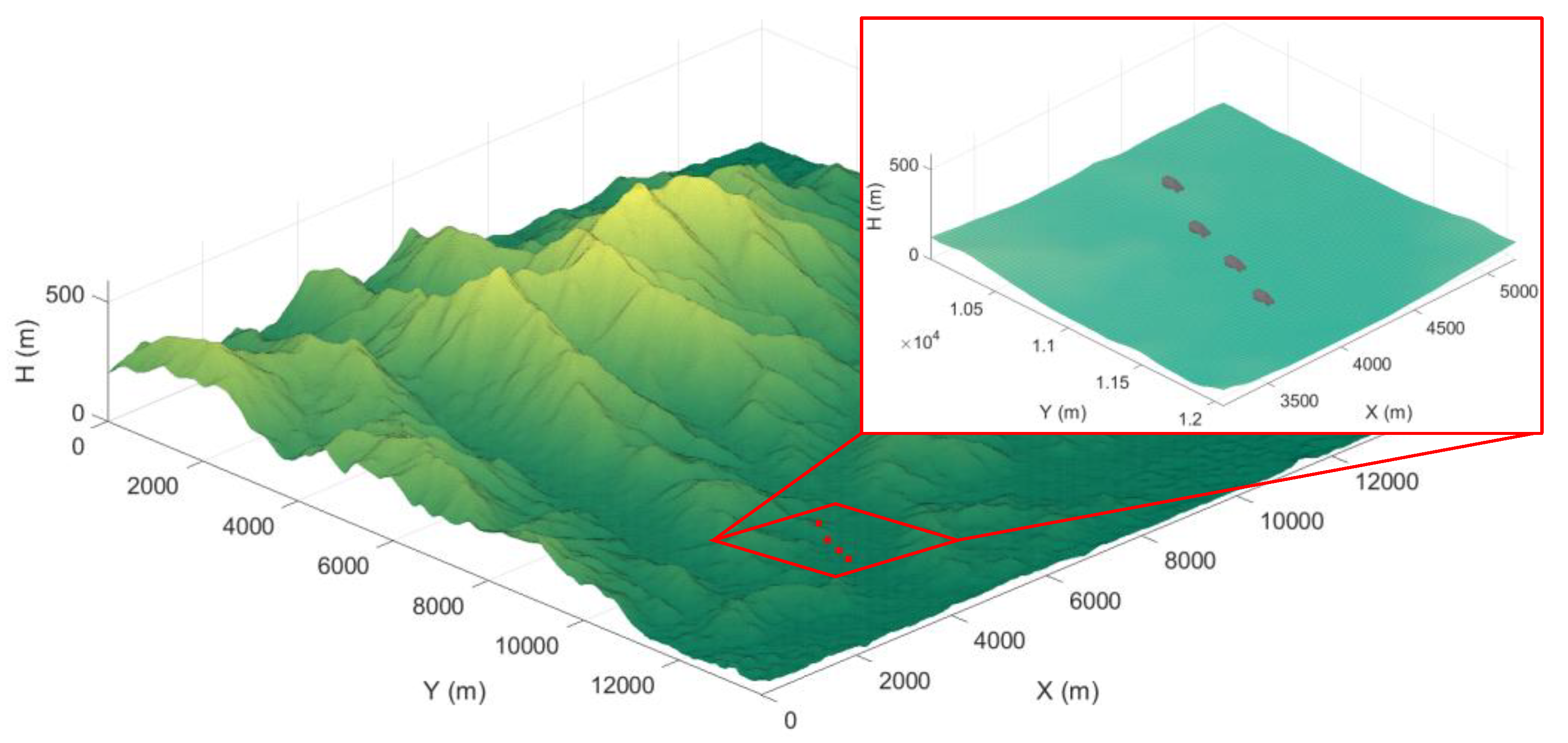
The targets in the AI mission scenario are shown in
Figure 8 with the detailed location coordinates are represented in
Table 2. The targets are assumed to be parked enemy vehicles.
Figure 9 illustrates the planned path of the AI mission scenario. The red transparent spherical area represents randomly placed threats, and the transparent cube area represents the target intercept mission area. The mission proceeds in order, starting with the triangle point and passing through the square point, the pentagonal point, and the hexagonal point, while the exact coordinates are shown in
Table 3. The targets are represented by x points and the threat properties are shown in
Table 4.
The total consumed time is 30.6 s, and the number of samplings is set as 5000 for each terrain flight path planning for AI mission planning. As shown in
Figure 9, the path is appropriately generated to avoid the threats while intercepting targets with the shortest length. Furthermore, the path is generated within 100 m above the surface in the terrain flight phase.
5.2. SEAD Mission Scenario
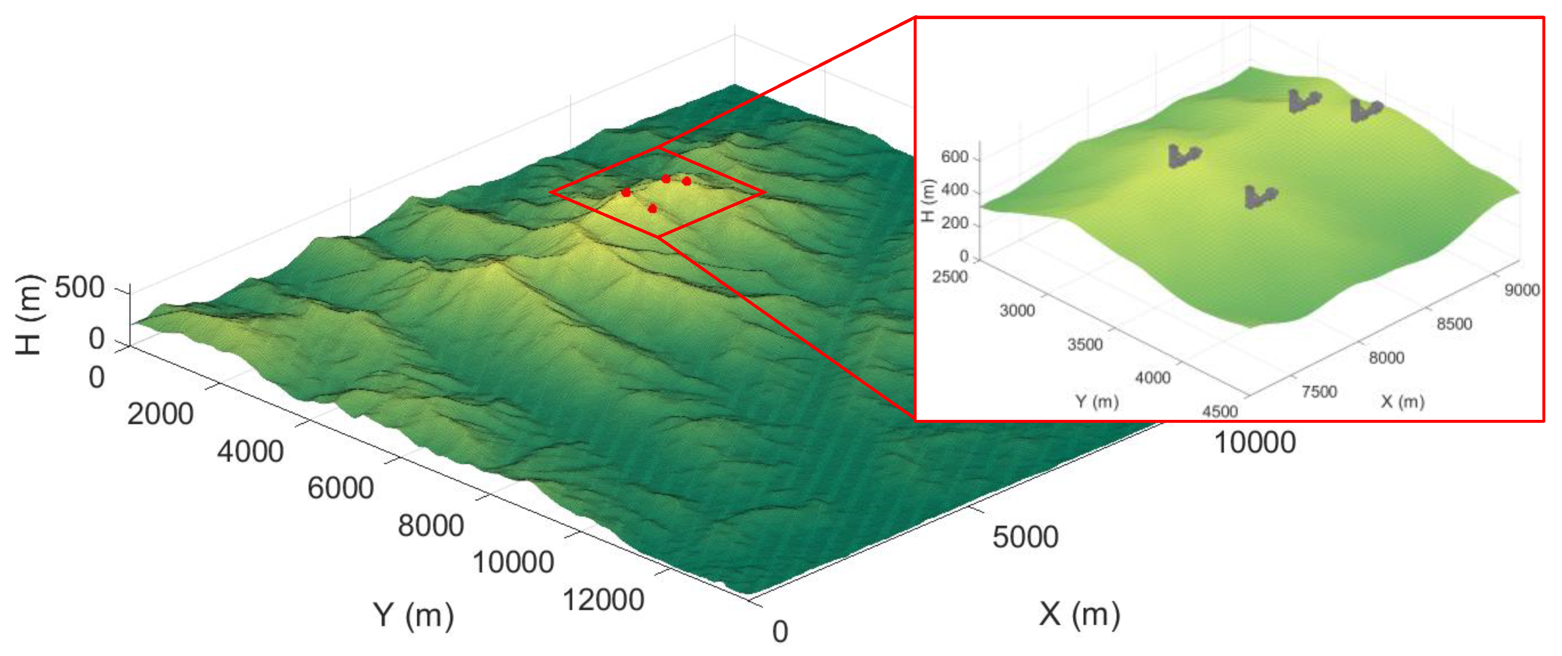
Figure 10 shows the targets of the SEAD mission scenario. The targets are assumed as already deployed enemy air defense assets on the highlands. The total number of targets is four and the locations of the targets are shown in
Table 5.
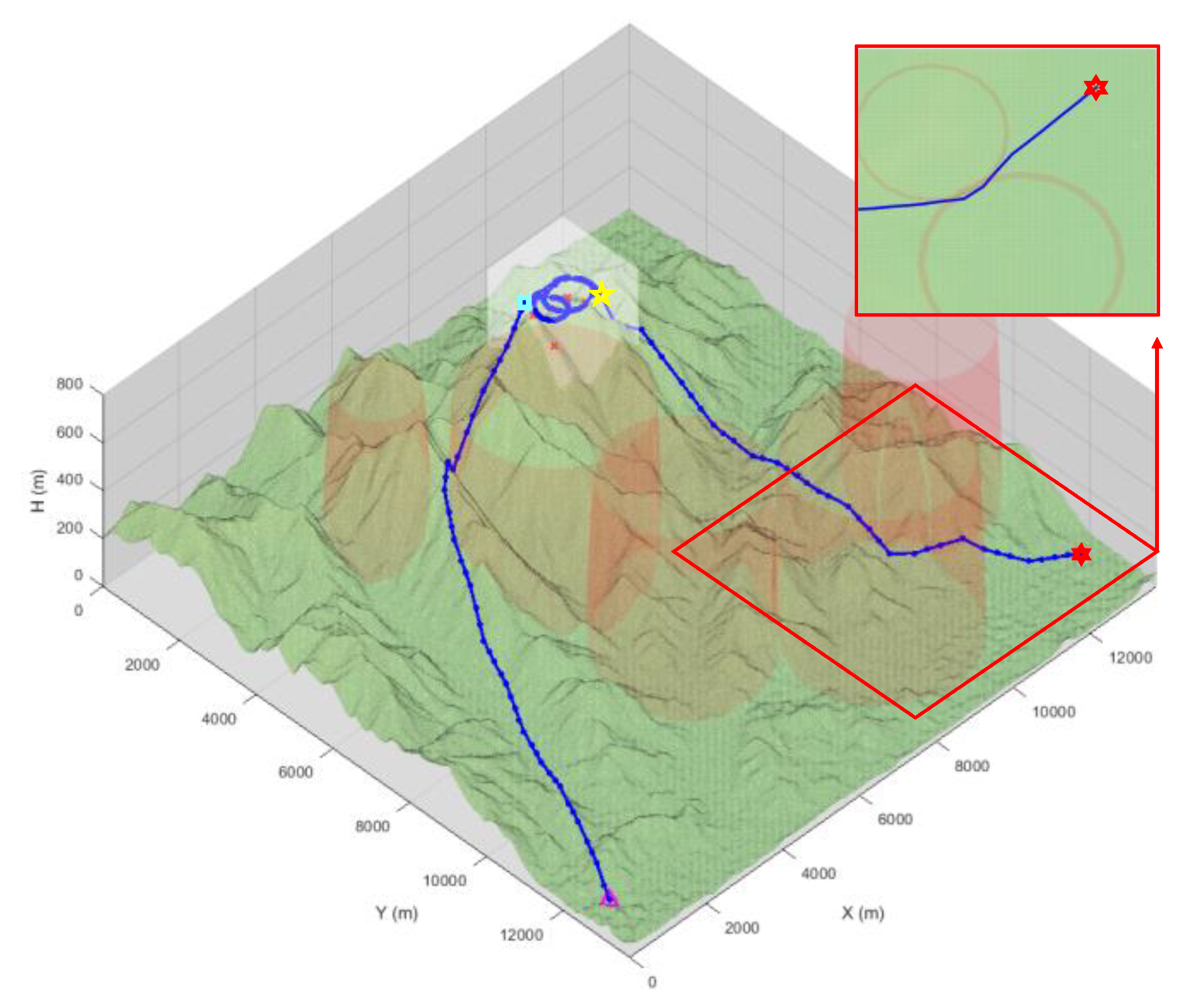
Figure 11 represents the planned path of the SEAD mission scenario. The red transparent spherical area represents randomly placed threats, and the transparent cube area represents the target intercept mission area. The mission proceeds in the following order: the triangle point, the square point, the pentagonal point, and the hexagonal point while the exact coordinates are shown in
Table 6. The targets are represented by x points and the threats’ properties are shown in
Table 7.
The total consumed time is 16.85 s, and the number of samplings is set as 5000 for each terrain flight path planning for SEAD mission planning. The path shown in
Figure 11 avoids a threat with relatively strong strength near the hexagonal point. Furthermore, the path is generated within 100 m above the surface in the terrain flight phase. One can find that the highlighted path in
Figure 11 goes between threat #1 and threat #2 while bypassing a greater threat. This result occurs when it is more cost-effective to go through a threat than to avoid it.
6. Trajectory Tracking Simulation
Simulation of the planned trajectory tracking is essential to confirm the practical applicability of the proposed algorithm. Therefore, simulations are performed to track the flight trajectory as a function of time generated based on the planned path.
The waypoints represented in
Section 5 only contain the sequence of position vectors. However, the Flight Control System (FCS) which will be mentioned later, requires heading angle information as well as position vectors. Furthermore, this information must be given as a function of time. For these reasons, a series of processes of allocating time and heading angle to the waypoint and converting the path into functions of time is required. Arrival time at each waypoint is allocated by assuming that UCAV is flying in a straight line between each waypoint at a prescribed constant speed. Moreover, the heading angle at each waypoint is assigned to face the next waypoint. Additional waypoints can be assigned to describe the original path more precisely where the waypoints can be expressed as a function of time through 7th-order spline interpolation [
32]. The predicted arrival time may not be precise since the interpolated curve is not a straight line. To solve this problem, a simple iterative method is used to estimate the exact arc length and travel time simultaneously. Further details about trajectory generation are represented in Ref [
33].
In order to design an appropriate trajectory tracking flight control system, trajectory tracking performance, robustness against disturbances and uncertainties, and the operating range of the aircraft must be considered. Incremental Backstepping Control (IBSC) guarantees stability across all Operational Flight Envelopes (OFE) based on the Lyapunov stability theory and is not affected by mismatched uncertainty. For this reason, there have been many approaches to design a controller based on the IBSC concept [
34,
35,
36,
37,
38,
39,
40], and this paper also uses an IBSC-based tracking controller [
33]. The reference trajectory was directly used as a feedback signal to obtain excellent tracking performance. For the completeness of this paper, the controller presented in Ref. [
33] will be briefly described.
The main feature of the incremental control method is its stronger robustness compared to the conventional model-based control approaches. Rather than solely depending on the model dynamics, incremental controllers use the measurements of any aerodynamic changes through available sensors. Therefore, changes due to external disturbances or modeling errors can be measured and compensated directly to the controller, making the controller insensitive to such unfavorable effects. The aircraft’s equation of motion and the kinematic relations are defined as follows:
where
and
represent linear and angular velocity vector with respect to the aircraft’s body-fixed frame,
and
represent force and moment vector, and
and
represent the position and attitude vector of the aircraft. Furthermore,
and
are represented using the definition of the trigonometric functions like
and
for
as.
The second-order dynamics for (
) are derived as:
which can be represented as following second-order nonlinear equation:
where
is the primary control vector of a conventional helicopter consisting of the main rotor collective (
), lateral-cyclic (
), longitudinal-cyclic (
), and tail rotor collective(
. Let us define the dynamics in Equation (9) represented at
as:
By applying the Taylor’s series expansion to Equation (10) at
, and assuming
is small enough, the incremental dynamics can be derived as:
Since the rank the control effectiveness matrix
is less than the dimension of the system output
, the system is underactuated. To cope with such difficulty, the slack variable approach is adopted as in Ref. [
29] as follows:
where
and
are defined using the slack variable matrix
and the slack variable vector
as:
If is selected to make nonsingular, standard nonlinear control design methods can be applied to Equation (12).
The IBSC design starts by defining the trajectory tracking errors with the desired trajectory
as:
where
is the virtual control vector. Now, a control Lyapunov function
is defined.
Without further derivation, the IBSC law that stabilizes the above Lyapunov function (
) can be selected as:
where,
and
are diagonal, positive definite matrices composing controller gains, and
is a diagonal, positive definite matrix composing updating law gains. If you need further details of the controller, referring to Ref [
33] is recommended.
Rotorcrafts are more appropriate to perform low-flying contour chasing maneuvers than fixed-wing aircraft for their low-speed flyability. For this reason, the BO-105 helicopter nonlinear model, modeled using the HETLAS program [
41,
42], is utilized.
The trajectories are generated based on the AI mission and the SEAD mission paths in
Section 5.
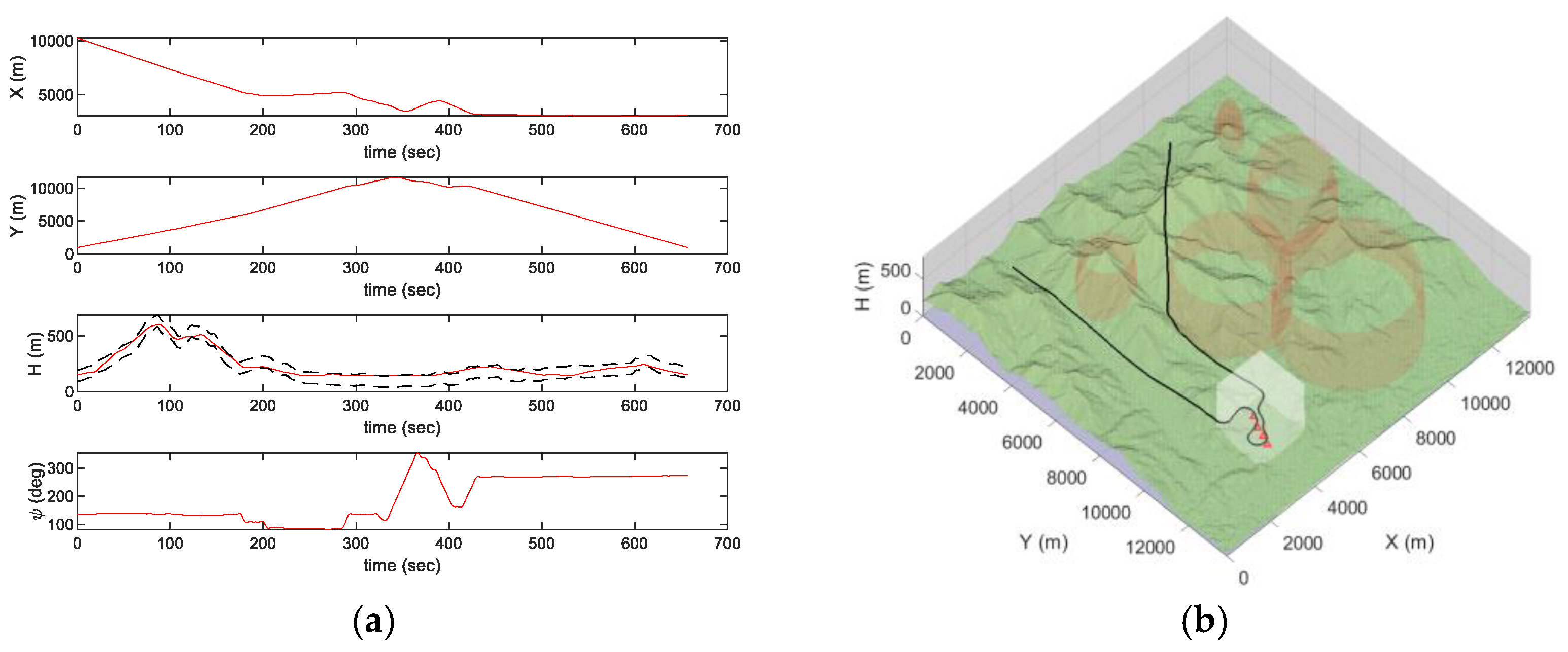
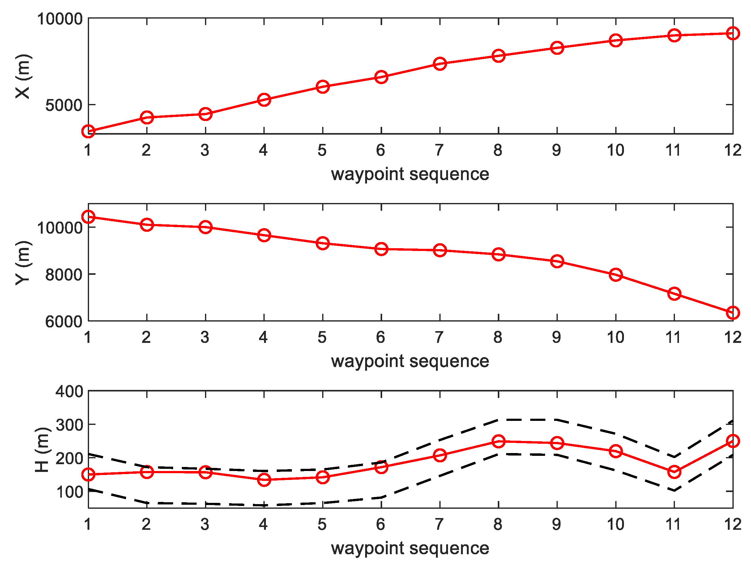
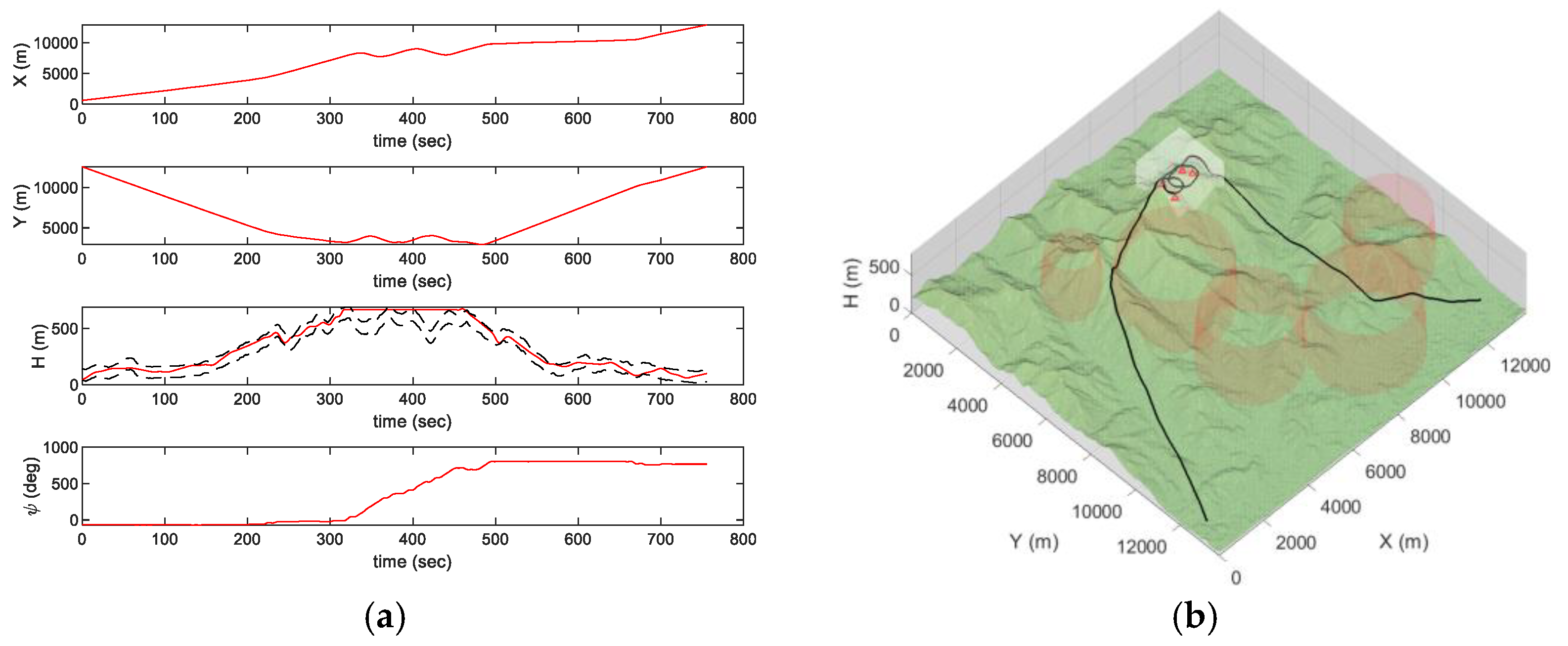
Figure 12 and
Figure 13 represent the generated trajectories to fly at a constant speed of 40 m/s. The dashed line represents the height limit boundary of the terrain flight. That is, the lower boundary indicates the ground surface, and the upper boundary indicates a line of 100 m above the surface. As shown in
Figure 12a, the height of the terrain flight trajectory was generated within 100 m from the surface. Meanwhile, the intercept maneuver trajectory was not affected the height constraint.
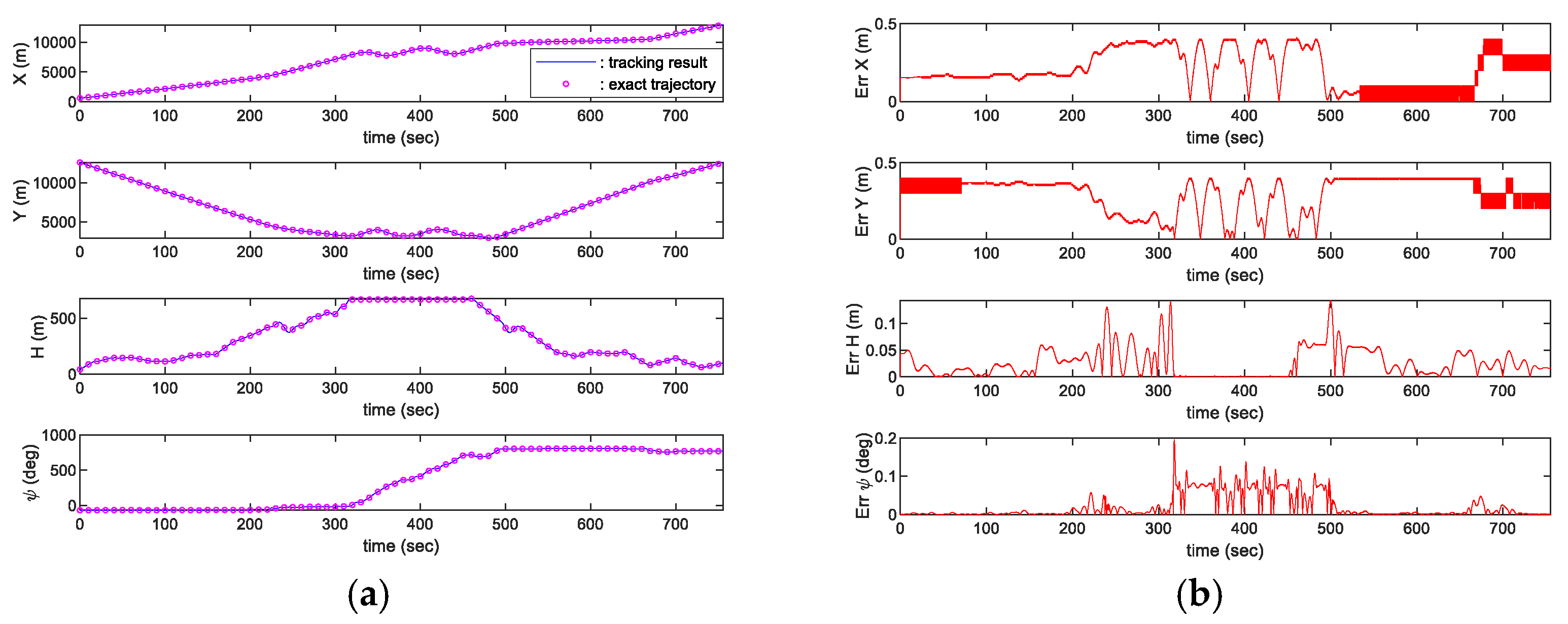
Figure 14 and
Figure 15 show tracking results and its error. Both results represent highly accurate tracking performance while showing position error within 1 m and heading angle error within 0.2 degrees. Through such high-accuracy tracking performance, the terrain flight missions can be performed without any collision.
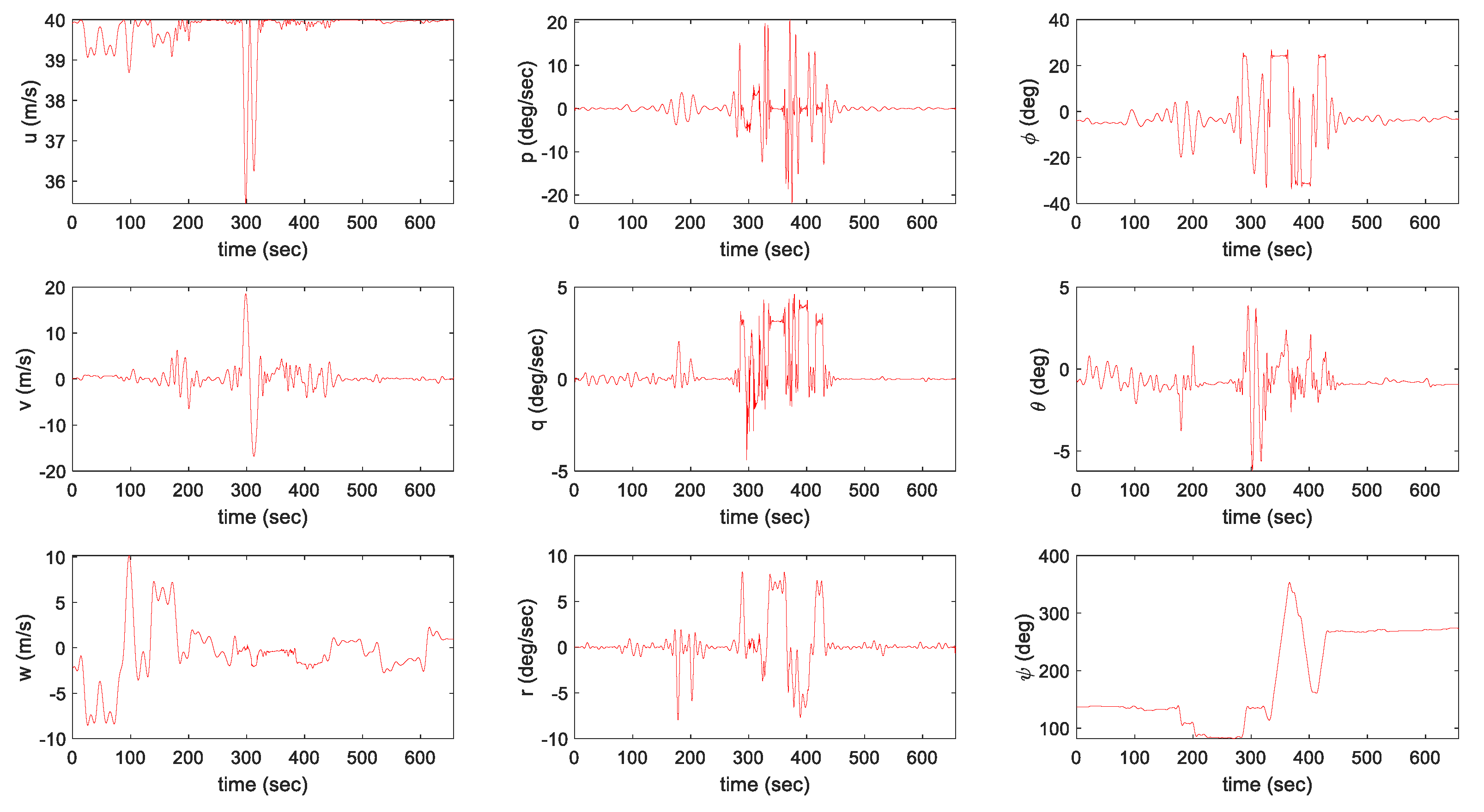
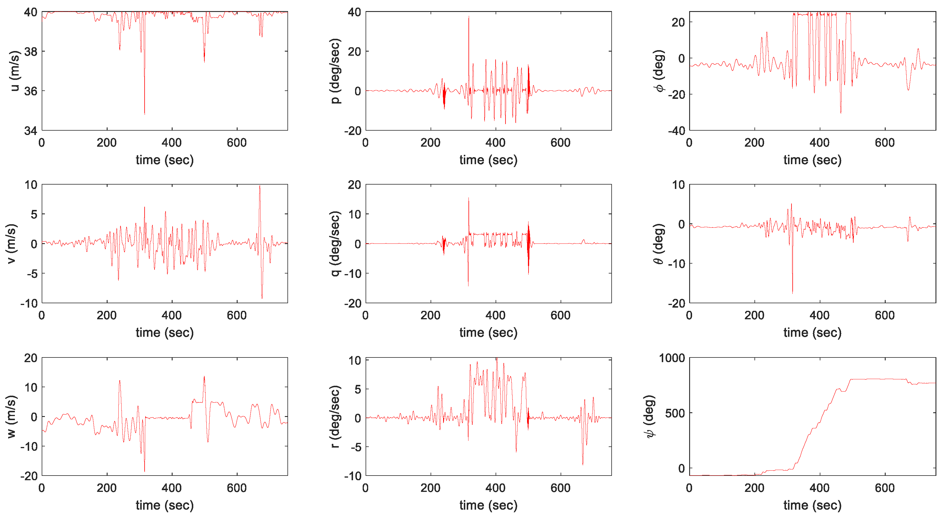
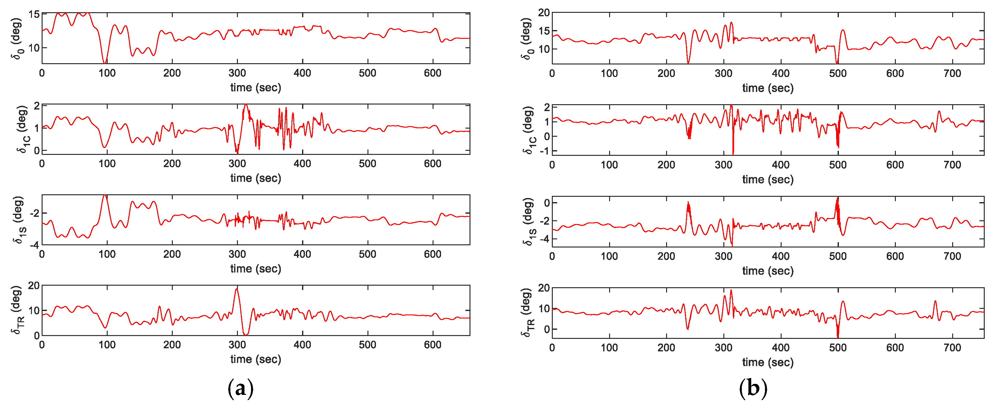
The control inputs and states during the simulation are represented in
Figure 16,
Figure 17 and
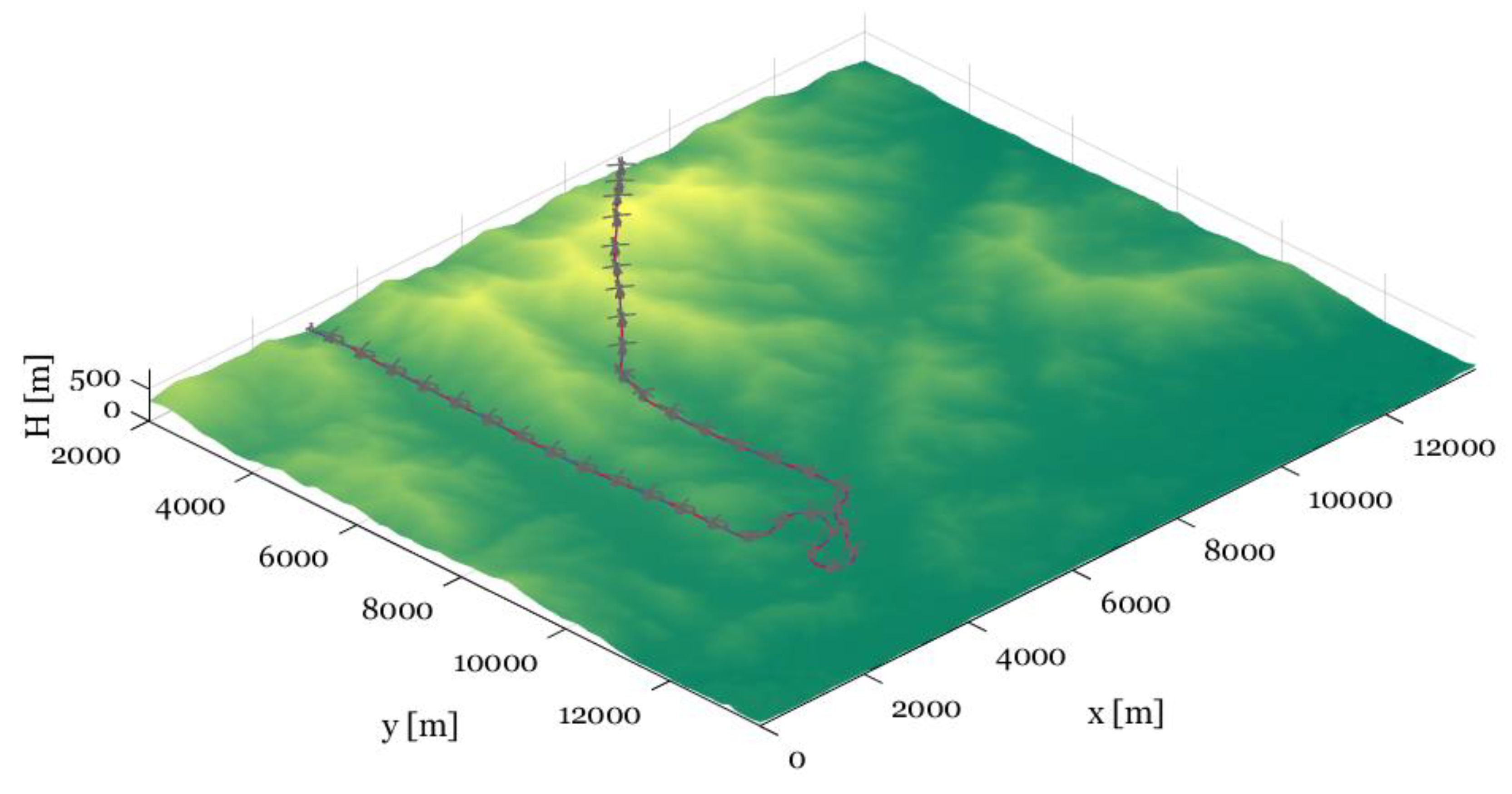
Figure 18. In the AI mission scenario, the lateral velocity varies over 40 m/s at about 300 s. Furthermore, the roll attitude temporally reaches over −30 degrees during intercept maneuver flight and the variation over 10 degrees in the pitch angle is represented at about 300 s. In the SEAD mission scenario, the lateral velocity varies over 40 m/s at about 650 s. Moreover, the roll attitude temporally reaches over 20 degrees during intercept maneuver flight and the variation over −15 degrees in the pitch angle is represented at about 320 s. The results in both simulations prove that the presented controller can maintain continuous tracking performance even with the aggressive maneuver. Furthermore, SEAD missions can be successfully performed with large height variations, where the maximum rate of climb reaches more than 10 m/s and the minimum rate of climb reaches near −20 m/s. In addition, the result is visualized in
Figure 19 and
Figure 20 to help discernible understanding.
7. Conclusions
A mission planner that enables effective ASM performance while considering the risk factors of the mission environment has been proposed and validated in this paper. First, ASMs were considered to consist of three sequential mission elements. The P-RRT*-smart algorithm was used to plan the ingress and egress mission element paths to quickly find the asymptotic global optimal path. The algorithm made it possible to find a path that could fly within 100 m of the surface. In addition, the concept of step cost was developed to account for the threats spread in the mission area. In order to increase the survivability of the UCAV and properly attack multiple targets, Dubins path was adopted in the intercept phase to generate short distance path near targets, taking into account the aircraft’s dynamic characteristics and the aiming capability of the mounted missiles. However, since the total length of the path still depends on target entry angles and the order of interception, the NLP was formulated to minimize the total length of the intercept path considering both the intercept entry angles and target intercept sequences. In return, the shortest intercept path could be obtained through the robust SQP. The integrated planner was then demonstrated in several test scenarios using a 3D terrain model with randomly placed threats. Finally, tracking simulations of the given path were successfully performed through a nonlinear rotorcraft model, confirming the method’s effectiveness.
Although the proposed planner has been confirmed to be an effective approach, questions about its real-time applicability remain. Therefore, there are several possible directions for the real-time applicability of this method. Since the proposed terrain path planner focuses on global planning, many samplings were performed in order to obtain the asymptotic optimal path. For this reason, the time consumed it takes to plan the terrain flight path shown in the results may seem quite long. In fact, the convergence time to the initial path and the optimal path was extremely short with in a few seconds. This characteristic shows the possibility of improvement as a real-time local planner sufficiently with a little improvement. The real-time local planner is focused on avoiding dynamic obstacles and threats during missions. To perform this task, the RT-RRT* [
43] which is advanced for real-time application can be applied to the proposed planner. Furthermore, PQ-RRT [
26] and bidirectional approaches [
44] may also be useful to accelerate the convergence rate. Additionally, Line-of-Sight Path Optimization (LoSPO) technique [
33] is a preferable option as a strategy to shorten the convergence time to the optimal path. Likewise, other RRT-based approaches can be applied to further improve the algorithm for real-time local planners.
The shortest intercept path planning may seem unsuitable for real-time applications. However, the time consumed shown in the results is the time required for optimization by setting the initial values to 0. In this case, it may take a long time to converge. Therefore, a strategy of planning the path with the previously optimized value as the initial value during the flight may be effective.
The results show that the proposed planner can generate the optimal path to approach the targets and the shortest path to intercept targets on the 3D global map which is the major difference from the previous studies. Furthermore, the presented simulation results show that the applied controller tracks the planned trajectory with high tracking performance, which proves that the generated trajectories from the proposed planner are flyable. In addition, the robust controller is adopted to cope with uncertainties such as the instantaneous weight reduction that occurs during an armed drop. Therefore, the method proposed in this paper can greatly contribute to planning air-to-surface missions of autonomous UCAVs.


