UAV Obstacle Avoidance Algorithm to Navigate in Dynamic Building Environments

Abstract

In this work, a real-time collision avoidance algorithm was presented for autonomous navigation in the presence of fixed and moving obstacles in building environments. The current implementation is designed for autonomous navigation between waypoints of a predefined flight trajectory that would be performed by an UAV during tasks such as inspections or construction progress monitoring. It uses a simplified geometry generated from a point cloud of the scenario. In addition, it also employs information from 3D sensors to detect and position obstacles such as people or other UAVs, which are not registered in the original cloud. If an obstacle is detected, the algorithm estimates its motion and computes an evasion path considering the geometry of the environment. The method has been successfully tested in different scenarios, offering robust results in all avoidance maneuvers. Execution times were measured, demonstrating that the algorithm is computationally feasible to be implemented onboard an UAV.

1. Introduction

In the last years, the use of UAVs (unmanned aerial vehicles), also known as drones, has increased exponentially. These vehicles have been introduced in many different engineering fields such as civil engineering [1,2] or photogrammetry and remote sensing [3] applications. Their reduced cost and versatility are the main reasons for the increase in their use. In most cases, UAVs are used for outdoor applications using remote sensing payloads such as RGB cameras or LiDAR sensors, but also for indoor applications.

In the civil engineering field, UAVs have been used for many different applications [4] such as safety monitoring, inspection tasks, or progress monitoring of the construction. For safety monitoring applications, they are a powerful tool to capture aerial images used to detect unsafe conditions and for monitoring the well-being of the workforce [5]. These applications have increased thanks to the introduction of different solutions that improve the autonomy of the UAVs [6]. Using a tethering power system [7] allows a drone to fly for days, making them a semi-permanent safety system. Furthermore, UAVs are already in use for construction progress monitoring [8] and for both indoor [9] and outdoor environments [10]. One example of construction monitoring using UAVs was shown in the work presented by Wu et al. [11], where an UAV equipped with a camera is used for the safety monitoring and analysis of foundation pit construction. In other cases, the UAVs are equipped with LiDAR (Light Detection and Ranging) sensors [12] using the acquired point cloud to monitor the construction process. In [13], Rebolj et al. introduced a method where the information obtained from the point cloud was used with the BIM model to automate progress monitoring.

UAVs are also a powerful tool to perform different kinds of structure inspections. Some of these tasks are focused on detecting superficial pathologies such as cracks or rust using remote sensors [14]. In recent years, new UAV systems have been developed to perform contact inspection tasks to detect internal pathologies in the structure using contact NDT sensors such as ultrasonic sensors [15,16].

Taking all this into account, it can be deduced that in the future, new civil engineering and construction applications will be created where drones will navigate in dynamic scenarios, that is, spaces shared with other vehicles, machinery, humans, or objects in movement. In this new scenario, new safety protocols and tools are going to be crucial to avoid risks. Jeelani et al. [17] presented a safety assessment of the integration of UAVs in construction environments. In this study, authors defined three different risks: physical risks, attentional costs, and psychological impacts.

The present work focused on this first risk by developing an obstacle avoidance system able to reduce or avoid the risk of collision between the UAV and objects or humans that get in the way of the planned mission inside a building. Many different approaches have been proposed in recent years on this subject. Some of the most common are based on geometric relations [18,19], fuzzy logic [20,21], potential fields [22,23], and neural networks [24,25,26], among others. However, most of them are only valid for the avoidance of static objects in open air environments. Indoor scenarios are quite challenging due to the presence of multiple obstacles that complicate the use of analytical tools and deep learning techniques. Furthermore, the use of neural networks is clearly limited by the lack of training data and avoidance protocols. Besides, another troublesome aspect is the presence of moving obstacles such as persons. The avoidance algorithm must be able to predict their motion to establish a path that maximizes safety and effectiveness.

In this article, a solution based on optimal control is presented for the dynamic calculation of paths that allow us to solve those conflicts in real time. The proposed algorithm combines the information of the preregistered 3D model of the room with measurements taken by onboard sensors. The current implementation aimed to be embedded in an UAV with sensing devices such as a LiDAR or a stereoscopic camera, which are frequently used in indoor navigation [27,28,29]. These sensors would allow us to detect the presence of objects that are not in the room model. If an obstacle is detected, given the information obtained from the sensors, the proposed algorithm makes a prediction of their motion and recalculates the trajectory if the possibility of conflict appears.

Optimal control is used in many scientific and engineering applications such as the calculation of space missions [30,31,32,33], aircraft trajectory optimization [34,35,36], and economics [37,38] between many other applications. It involves the definition of a performance index that measures the optimality of a given solution according to certain criteria. For the case of this obstacle avoidance program, the objectives were to minimize both the deviation from the critical path and the time of the maneuver. The behavior of the algorithm can also be adjusted according to the characteristics of a given model of an UAV, prioritizing one of these objectives.

A direct approach to the optimal control problem was implemented as it allows one to obtain a robust and computationally inexpensive problem that can be solved by an onboard computer. Direct approaches rely on the Karush–Kuhn–Tucker conditions (KKT) [39], a generalization of the method of Lagrange multipliers that allows for the use of inequality constraints. For the implementation, a direct collocation was selected for the state variables, which were discretized in a time-grid. With the current formulation, a simple non-linear programming problem (NLP) is obtained, which allows us to reduce the computation time and be implemented in an onboard computer, as can be appreciated in the results.

Previous works that have used optimal control theory to solve air conflicts in civil aviation [34,35,36] optimized the trajectory of more than one aircraft and computed the required control inputs to minimize fuel consumption and avoid losing the separation minima among aircraft. Instead, apart from adapting the algorithm to the UAV characteristics, only one vehicle was considered, and obstacles were defined as external entities instead of being variables of the problem. Furthermore, a direct control over the state variables was imposed as control inputs were not the main object of study in this work. This is a much simpler implementation that only computes the reference trajectory of one vehicle, practically allowing the computation in real time and can be solved with a large-scale optimization algorithm, the Interior Point OPTimizer scheme (IPOPT). Further information can be found in the following reference on the implementation of this solver [40].

The main objective of this work was to develop a real time obstacle avoidance algorithm to allow future UAV applications in the civil engineering and construction fields, where these vehicles are going to have to navigate sharing space with humans and other objects. First, the algorithm must be able to predict the trajectory of moving objects to anticipate possible collisions during the navigation. Then, in the case of a collision prediction, the system computes a modification of the scheduled path to avoid the conflict, optimizing it in terms of deviation in time and position from the planned route.

The proposed algorithm departs from the results obtained in a previous work [41], in which a 3D path planning algorithm for indoor navigation was developed using a modification of the A* algorithm [42]. The previous work calculated the shortest path between two points inside an indoor scenario, specifically designed to perform completely autonomous contact inspection tasks with UAVs. For that, the scenario was pre-registered using as the only input a point cloud recorded by different kinds of LiDAR scanners such as terrestrial laser scanners (TLS) or mobile laser scanners (MLS). Each point cloud was discretized into obstacles using a voxelization.

The rest of this manuscript is organized as follows. Section 2 presents the developed methodology, going deep into the optimization problem. In Section 3, the results of different study cases are presented and discussed. Finally, Section 4 presents the conclusions of the proposed algorithm, and future works are introduced.

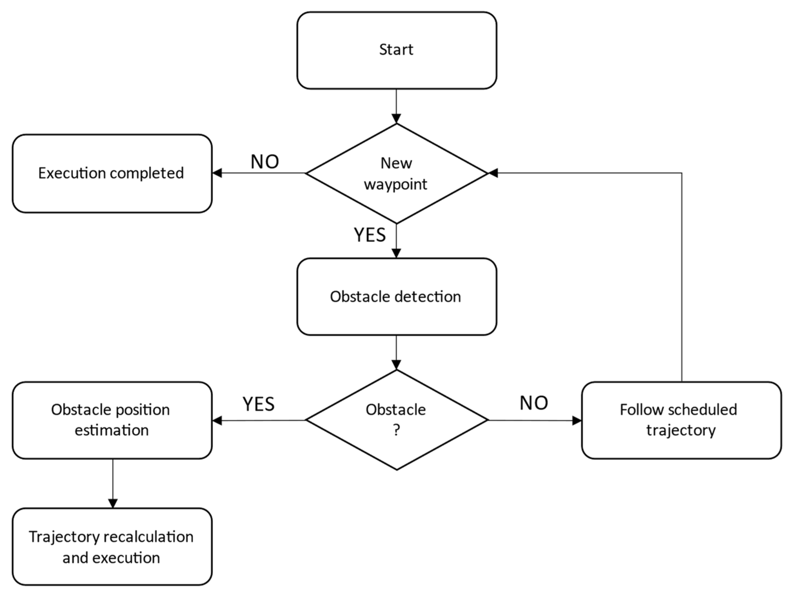
2. Methodology

For the implementation of the algorithm, different study cases were simulated in indoor environments, generated from pre-processed point clouds of rooms from the University of Vigo. The UAV trajectory was simulated as well as the obstacle detection and avoidance algorithm proposed in this manuscript. In the test scenario, the UAV flies on a route defined by waypoints. The drone has sensors onboard that allow for the detection of the presence of objects that are not in the original 3D model from the room.

A scheme of the implementation is presented in Figure 1 in the form of a decision tree. The same procedure is applied when the UAV reaches a waypoint of the trajectory. First, the drone takes samples of the room to detect whether there are any obstacles, and if so, it registers its position during a certain period of time, otherwise, the scheduled trajectory is followed. If a new obstacle is detected, a polynomial regression is performed, fitting the measurements of the sensors, to forecast its future position. Furthermore, a security distance is assigned as a function of the size and speed of the object. The position of this new obstacle is introduced into the optimization program, which recomputes the new trajectory profile considering its presence and using as the initial guess for the iterative method, the scheduled trajectory. The process finishes once the UAV reaches the final waypoint of the trajectory. As well as the trajectory of the UAV, the motion of these obstacles and the sampling process of the sensors are simulated, as explained in Section 2.2.2.

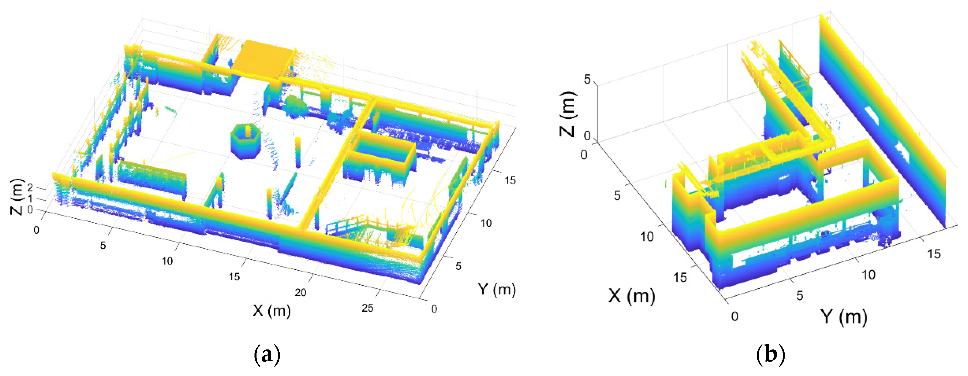
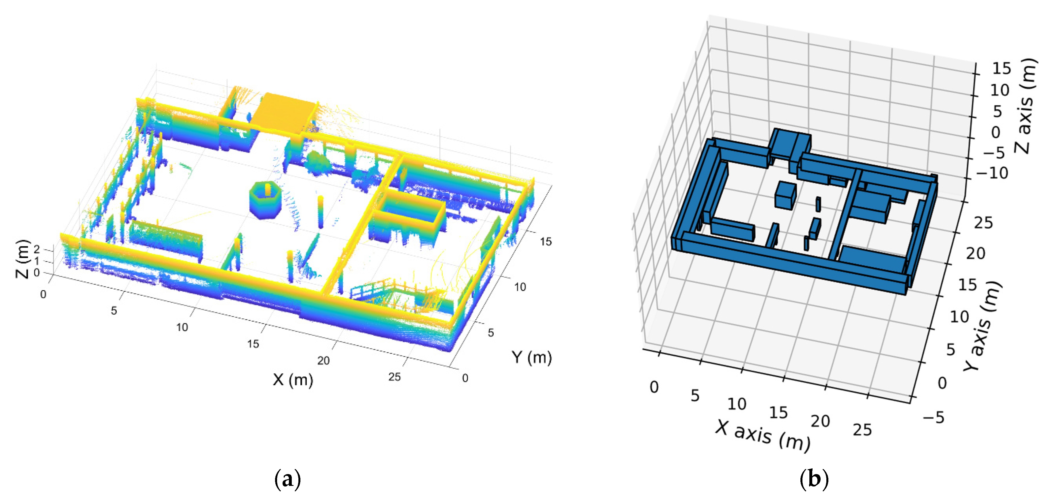
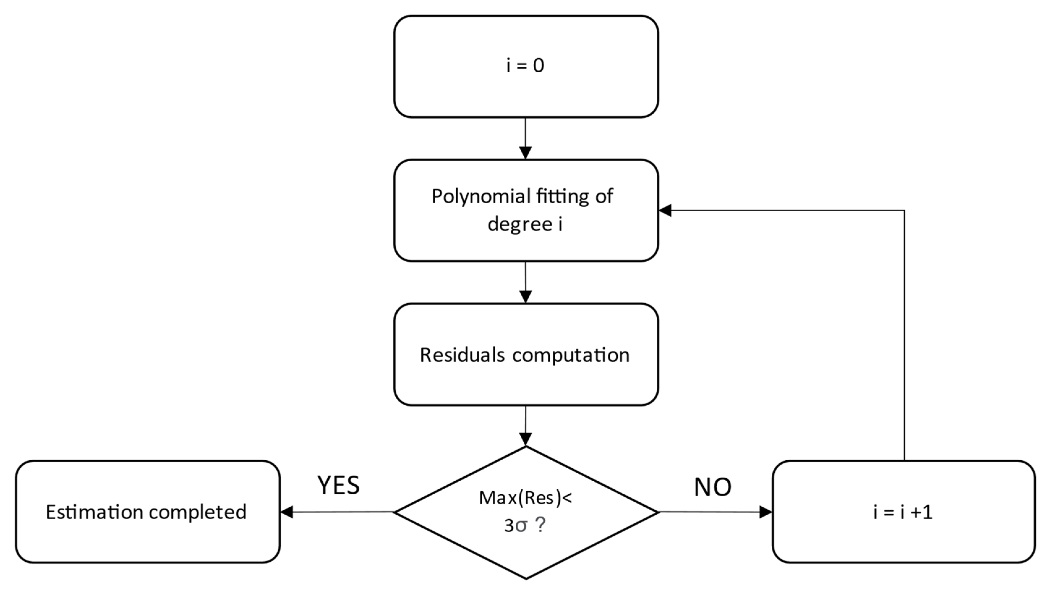
2.1. Scenario Discretization

In this article, two scenarios are presented to show the capabilities of the proposed algorithm in different environments, showing the adaptability to different types of flight conditions.

• Hall of the School of Mining and Energy Engineering at University of Vigo. It is a scene with many obstacles and a low ceiling, in which it is practically impossible to overfly any obstacle (Figure 2a). This point cloud was captured with the MLS ZEB-REVO laser scanner [43].
• MTI (Industrial Technology Module). It is an industrial warehouse of the University of Vigo, a much wider room with a high ceiling (approximately 5 m high). Flying over obstacles will be tested in this room (Figure 2b). This point cloud was acquired with the TLS Faro Focus 3D X330 laser scanner [44].

Figure 2. Scenarios. (a) Hall of the School of Mining and Energy Engineering. (b) MTI.

Figure 2. Scenarios. (a) Hall of the School of Mining and Energy Engineering. (b) MTI.

The point clouds were postprocessed to obtain a discretized version of the room environment suitable for the optimization scheme. First, they were segmented, clustering the walls and the inner obstacles into individual clouds. Then, these clouds were fitted into rectangular prisms defined by a central point and the dimensions of their sides (Figure 3).

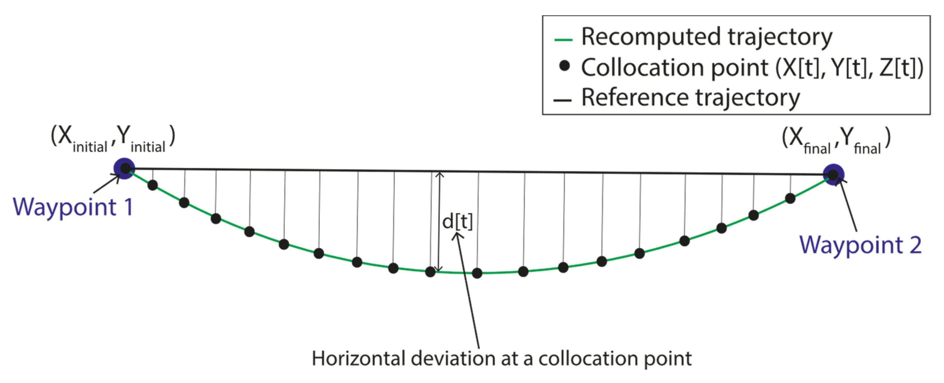
2.2. Optimal Control Problem Formulation

Optimal control involves the minimization of a cost function that is typically a function of the state and control variables. In this implementation, a direct control over the state variables was imposed, as this obstacle avoidance is meant to define a reference path profile, but not the control inputs that are specific to each model of UAV and typically adjusted by the flight controller. The current implementation is aimed to reduce the complexity of the algorithm to allow for real time calculations. Therefore, the defined cost function only depends on the state variables (Equation (1)). It is composed of two terms: the first one, the Mayer term, and the second one, the Lagrangian, which involves the computation of an integral. The statement of a generic optimal control with no control inputs is as follows:

$$J\left(x,t_0,t_f\right) =E \left[x\left(t_0\right),t_0 , x\left(t_f\right), t_f\right] +{{\displaystyle \int }}_{t_0}^{t_f}F\left[x\left(t\right),t\right]dt$$

(1)

where x(t) denotes the set of state variables of the optimal control problem subject to:

$$\begin{gathered} \mathrm{Dynamic}\mathrm{constraints}:\dot{x}\left(t\right) =f\left(x\left(t\right),t\right) \\ \mathrm{Initial}\mathrm{conditions}:i\left(x\left(t_0\right),t_0\right) =0 \\ \mathrm{Final}\mathrm{Conditions}:e\left(x\left(t_f\right),t_f\right) =0 \\ \mathrm{Algebraic}\mathrm{path}\mathrm{constraints}:g\left(x\left(t\right),t\right) =0 \end{gathered}$$

(2)

To solve this time-continuous problem, a direct approach was implemented. The trajectory in Cartesian coordinates is sampled in a discretized time-grid (Equation (3)). The number of collocation points is a parameter that can be defined by the user, or adapted dynamically, depending on the required spatial and temporal resolution. In this way, the set of coordinates for the temporal steps can be grouped in the following arrays of decision variables:

$$\begin{gathered} \mathit{X}= \left[X\left[1\right],X\left[2\right],\dots ,X\left[nstep\right]\right] ; \mathit{Y}= \left[Y\left[1\right],Y\left[2\right],\dots ,Y\left[nstep\right]\right] ; \\ \mathit{Z}= \left[Z\left[1\right],Z\left[2\right],\dots ,Z\left[nstep\right]\right] \end{gathered}$$

(3)

The temporal array is defined in an evenly spaced set of time steps as a function of the time of execution of the maneuver $t_f$(Equation (4)):

$$t= \left[0,\mathsf{\Delta }t,2\mathsf{\Delta }t\dots ,t_f\right];\mathsf{\Delta }t=\frac{t_f}{nstep-1}$$

(4)

The objective function is obtained through a discretization of Equation (1) in the time steps of the grid. Regarding the Mayer term, a squared difference between the scheduled time of flight and the calculated one was selected. The Lagrangian term is represented by a summation that accounts for the squared deviation of the grid points with respect to the linear reference trajectory (Equation (5)). Two parameters, a and b, are introduced to tune the response of the algorithm. Higher values of a will prioritize faster trajectories, maximizing the speed to reach the final waypoint at the scheduled time ($t_{fscheduled})$. The latter, b, controls the horizontal deviation from the nominal trajectory at the discretization points, as depicted in Figure 4. The larger the value of b, the straighter the trajectory will be, regardless of the time of flight. A parametric study of the influence of this parameter was performed to demonstrate the adaptation capabilities to different types of UAV:

$$J\left(\mathit{X},\mathit{Y},\mathit{Z},t_f\right) =a{\left(t_f-t_{fscheduled}\right)}^2+\frac{b}{nstep} {\displaystyle \sum }_{t=1}^{nstep}\frac{{\left(\left(X_{initial}-X_{final}\right)\left(Y\left[t\right] - Y_{final}\right) - \left(Y_{initial}-Y_{final}\right)\left(X\left[t\right] - X_{final}\right)\right)}^2}{\left({\left(X_{initial}-X_{final}\right)}^2+{\left(Y_{initial}-Y_{final}\right)}^2\right)}$$

(5)

where $\left(X_{initial}, Y_{initial}\right), \left(X_{final}, Y_{final}\right)$ are the coordinates from the initial and final waypoint. These values, along with the corresponding height for the Z coordinate, are introduced as constraints for the initial and final collocation point of the trajectory, as shown in Figure 4.

In the following sections, the discretized constraint Equation (2) that complete the non-linear programming problem will be introduced.

2.2.1. Dynamic Constraints of the Vehicle

The first constraints of this problem are the performance capabilities of the vehicle. Maximum speeds (Equation (6)) and accelerations (Equation (7)) must be limited to meet the flight capabilities of a certain model of UAV. For simplicity and reduction in the computation time, in this formulation, instead of considering decision variables for acceleration and speed, these dynamic constraints were introduced derived from first order forward differences and second order central differences. This allows us to reduce the number of variables of the problem and hence the times of computation:

$$\forall t : {\left(X\left[t+1\right] - X\left[t\right]\right)}^2+{\left(Y\left[t+1\right] - Y\left[t\right]\right)}^2+{\left(Z\left[t+1\right] - Z\left[t\right]\right)}^2-V_{max}^2\mathsf{\Delta }{t}^2\le 0$$

(6)

$$\begin{array}{ll}\forall t : (X\left[t+1\right] - & 2X\left[t\right] + X\left[t-1\right]{)}^2+{\left(Y\left[t+1\right] - 2Y\left[t\right] + Y\left[t-1\right]\right)}^2\\ & +{\left(Z\left[t+1\right] - 2Z\left[t\right] + Z\left[t-1\right]\right)}^2-a_{max}^2\mathsf{\Delta }{t}^4\le 0\end{array}$$

(7)

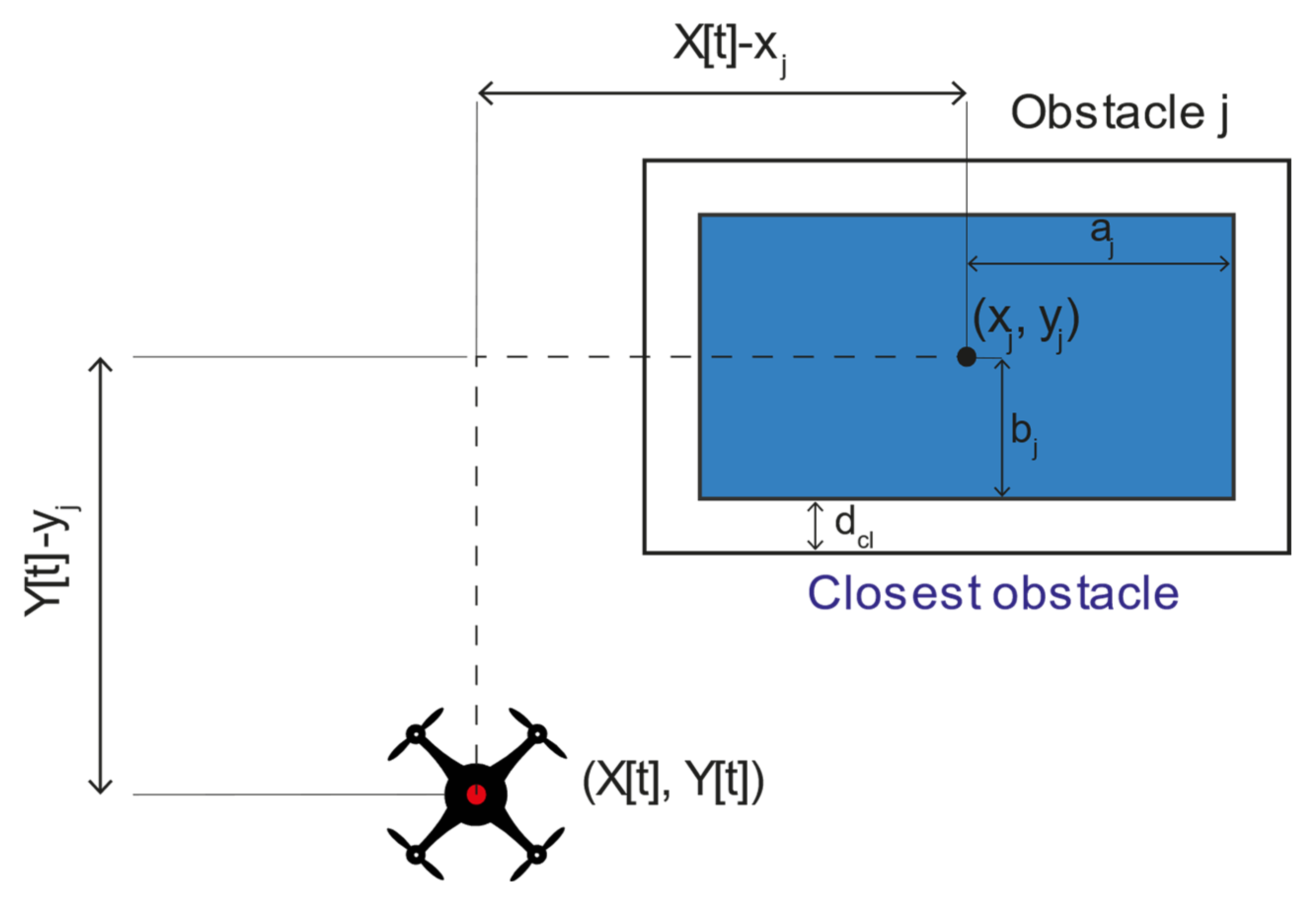
2.2.2. Algebraic Constraints

The physical surroundings of the UAV are introduced to the algorithm as algebraic constraints that represent those positions in which the UAV must not penetrate. This section is divided into two subsections: (1) room scenario, which accounts from the obstacles pre-recorded in the 3D point cloud; and (2) unrecorded and moving obstacles, those that were not present in the acquired point cloud but detected by the onboard sensors during the navigation.

• Room scenario

As previously mentioned, the walls and obstacles were discretized using rectangular prisms. The numerical scheme has a set of prohibited space regions in which the UAV must not penetrate to avoid collisions with objects placed in the navigation area. These are defined given the centers and dimensions of the sides of the prisms (Equation (8)). For every point of the trajectory, the following equation shall be fulfilled:

$$\forall t: \frac{min}{j in obs}\left(max\left(\frac{abs\left(X\left[t\right] - x_j\right)}{a_j+d_{cl}},\frac{abs\left(Y\left[t\right] - y_j\right)}{b_j+d_{cl}},\frac{abs\left(Z\left[t\right] - z_j\right)}{c_j+d_{cl}}\right)\right) - 1\le 0$$

(8)

A modified version of the norm infinity was employed to model the rectangular geometry of the obstacles, as illustrated in Figure 5. The parameters $a_j$, $b_j$, and $c_j$ represent the half of the side of each dimension of the prism j and ($x_j,y_j,z_j)$, the Cartesian coordinates of the centers whereas $d_{cl}$ is a security distance associated with uncertainties. To reduce the order of magnitude of the gradient vector and Hessian matrix of the problem, logical evaluation was performed to identify the closest obstacle to the trajectory. This allowed us to considerably reduce the number of constraints of the problem. Instead of having N constraints for each time step (given by the total number of prisms of the room, N), the problem is reduced to a single constraint and a logical evaluation.

The floor and ceiling of the building were not included in the discretization of the room. Instead, the range of allowable flight heights (Equation (9)) is restricted to a certain range given by:

$$\forall t :0\le Z\left[t\right] \le h_{max}$$

(9)

• Unrecorded and moving obstacles

As aforementioned, the UAV records the position and size of the obstacles of the room prior to the initialization of the avoid maneuver. It takes samples during a certain period of time and then, the algorithm performs a polynomial regression. In this manuscript, the trajectory of the obstacles and size was simulated. To represent the errors on the measurements, a Gaussian noise of typical deviation $\mathsf{\sigma }$ was added to the simulated trajectory of the obstacle. A decision tree methodology was developed to select the order of the polynomial. A high order one would overfit the measurements from the sensors, whereas a low order one would not correctly represent the motion of the obstacle. A scheme was implemented based on the residuals of the regression. This is initialized fitting the data to a zero-order polynomial (constant). As depicted in Figure 6, the residuals can then be calculated. If the maximum residual is higher than three times the typical deviation of the Gaussian distribution, the order of the polynomial is increased until the stop criteria is satisfied.

Finally, after applying the regression, the position of the obstacle in each time step (Equation (10)) is defined as a function of the regression coefficients, the time step $\mathsf{\Delta }t$, and the step number:

$$\begin{gathered} X_{obs}\left[t\right] ={}_{i=0}{}^n \sum c_{xi}{\left(t\mathsf{\Delta }t\right)}^i;Y_{obs}\left[t\right] ={}_{i=0}{}^n \sum c_{yi}{\left(t\mathsf{\Delta }t\right)}^i;Z_{obs}\left[t\right] \\ ={}_{i=0}{}^n \sum c_{zi}{\left(t\mathsf{\Delta }t\right)}^i \end{gathered}$$

(10)

Given the position of the central point of the obstacle, a new set of constraints can be defined for every time step of the discretization (Equation (11)). The distance from the UAV to the obstacle should not be lower than a given value $d_{safety}^2$ and can be adjusted dynamically depending on the size and speed of the obstacle.

$$\forall t:{\left(X_{obs}\left[t\right] - X\left[t\right]\right)}^2+{\left(Y_{obs}\left[t\right] - Y\left[t\right]\right)}^2+{\left(Z_{obs}\left[t\right] - Z\left[t\right]\right)}^2\le d_{safety}^2$$

(11)

3. Results and Discussion

3.1. Study Cases

Once the algorithm was developed, several tests were designed to study the behavior of the algorithm in different situations. The original route defined by waypoints was generated using the procedures described in [41], as depicted in Figure 7. A generic UAV with a maximum acceleration of $1 \mathrm{m}/{\mathrm{s}}^2$ and speed limited to $2 \mathrm{m}/\mathrm{s}$ was used for the simulations. Regarding the safety distance to the obstacles, a value of 1 m was used. Note that all the mentioned quantities are not intended to represent any commercial model of UAV, but are only test values to study the capabilities of the algorithm.

The first four test cases were simulated in the Hall of the School of Mining and Energy Engineering from the University of Vigo, a room with a low ceiling that does not allow for the vertical avoidance of obstacles. The equations of motion were constrained only to horizontal displacements. The UAV started the mission in waypoint 1, stopped at waypoint 2 to detect and evaluate the motion of the moving obstacle, and finally, recalculated a new avoidance trajectory to reach point 3 without causing a collision.

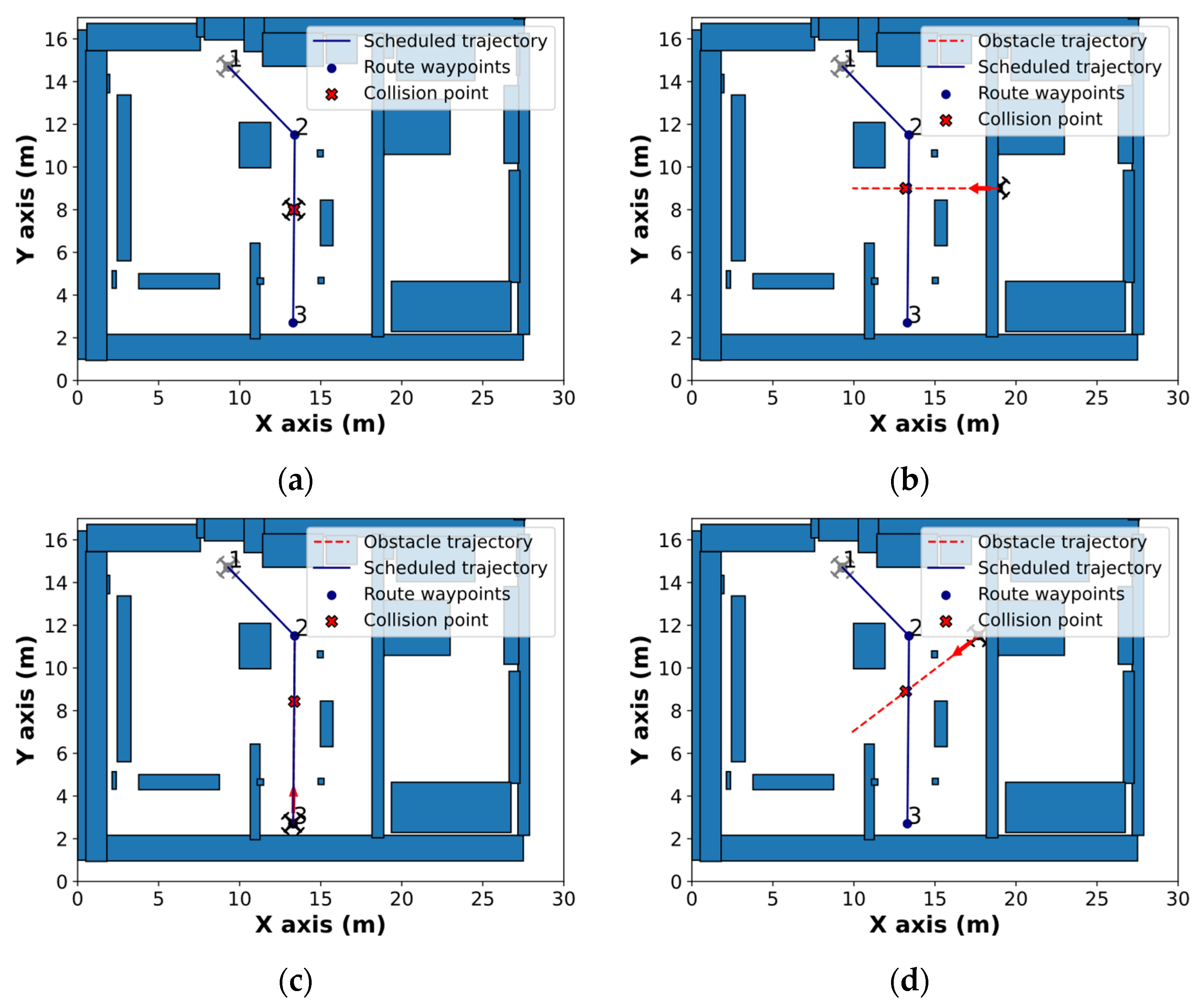
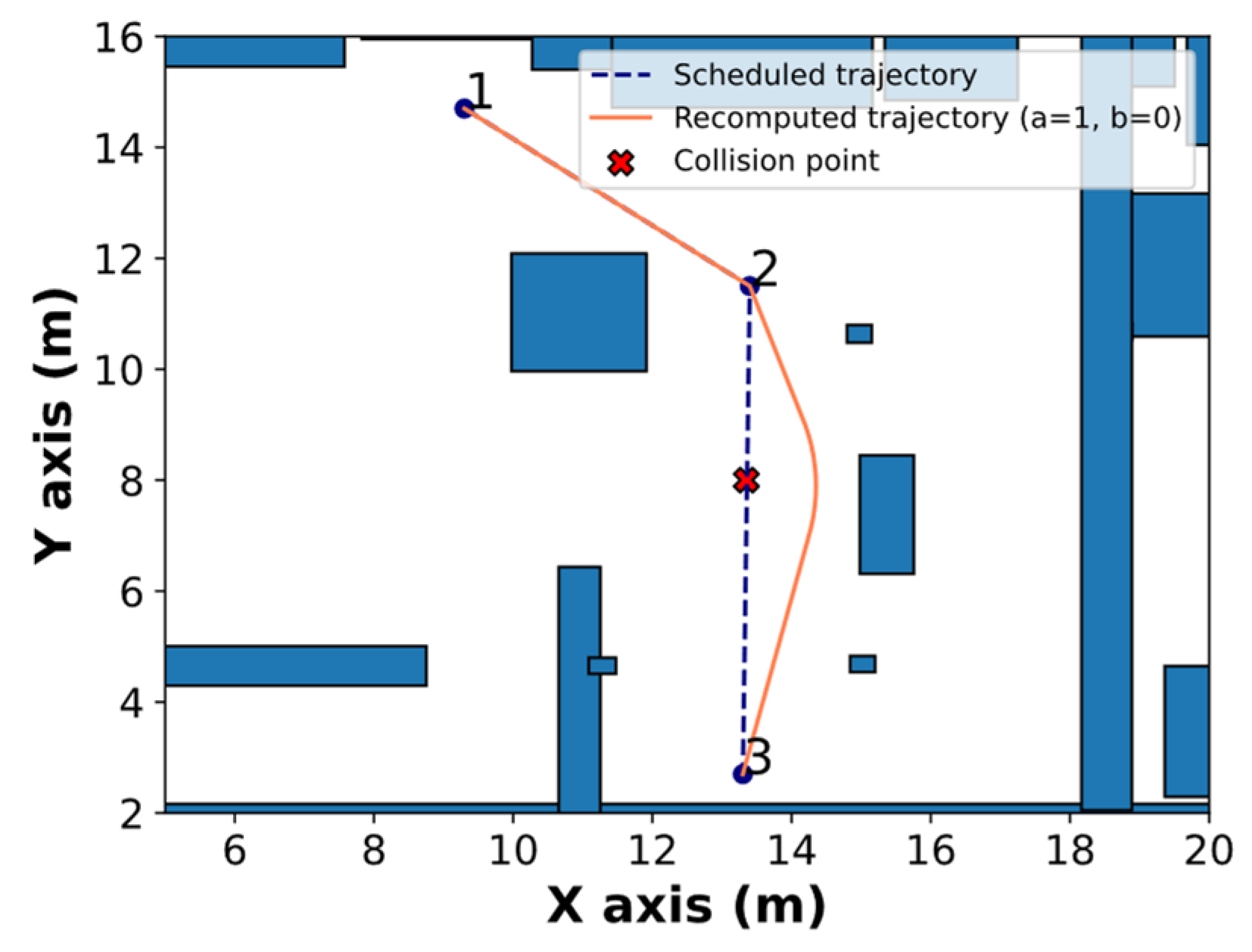
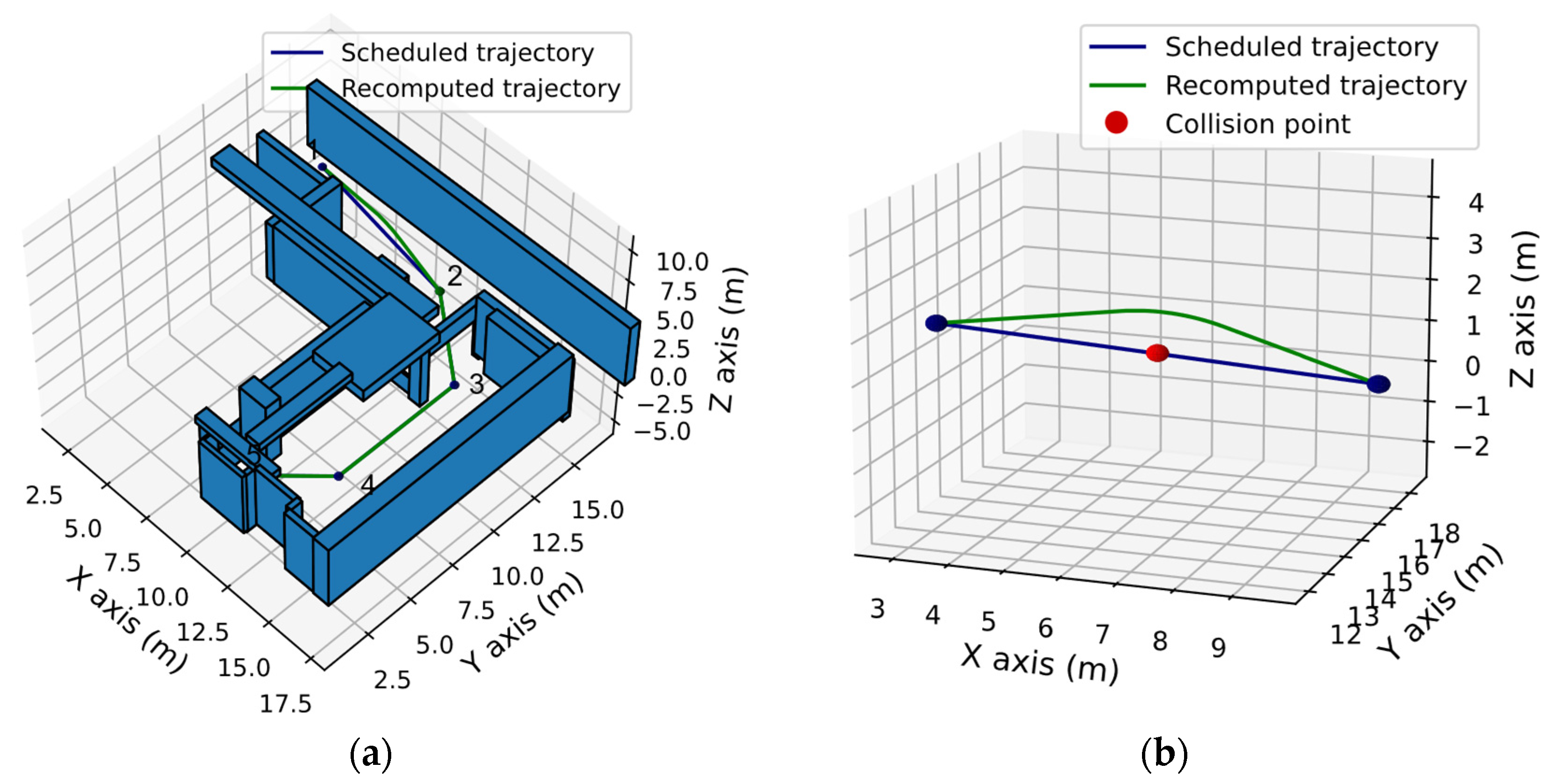
• Static obstacle: The first maneuver to be tested is a single static obstacle placed in the middle of the scheduled trajectory.
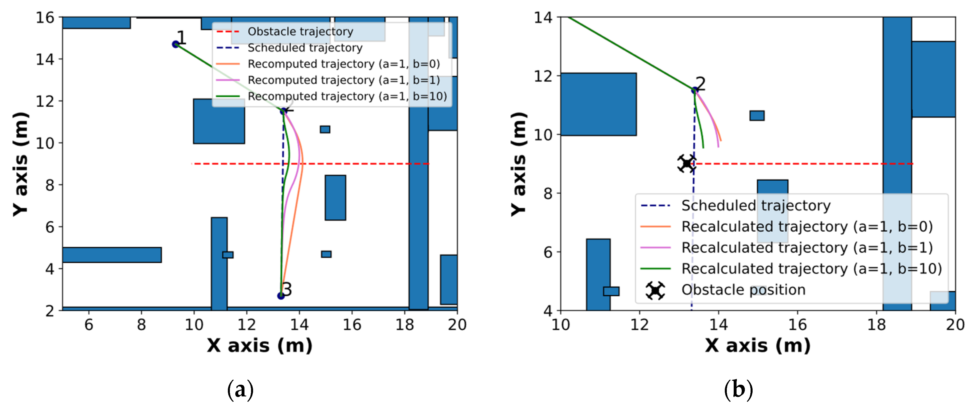
• Perpendicular moving obstacle: In this case, the object is moving perpendicularly to the obstacle at a constant speed of 1 m/s, intercepting the UAV in a point of the trajectory.
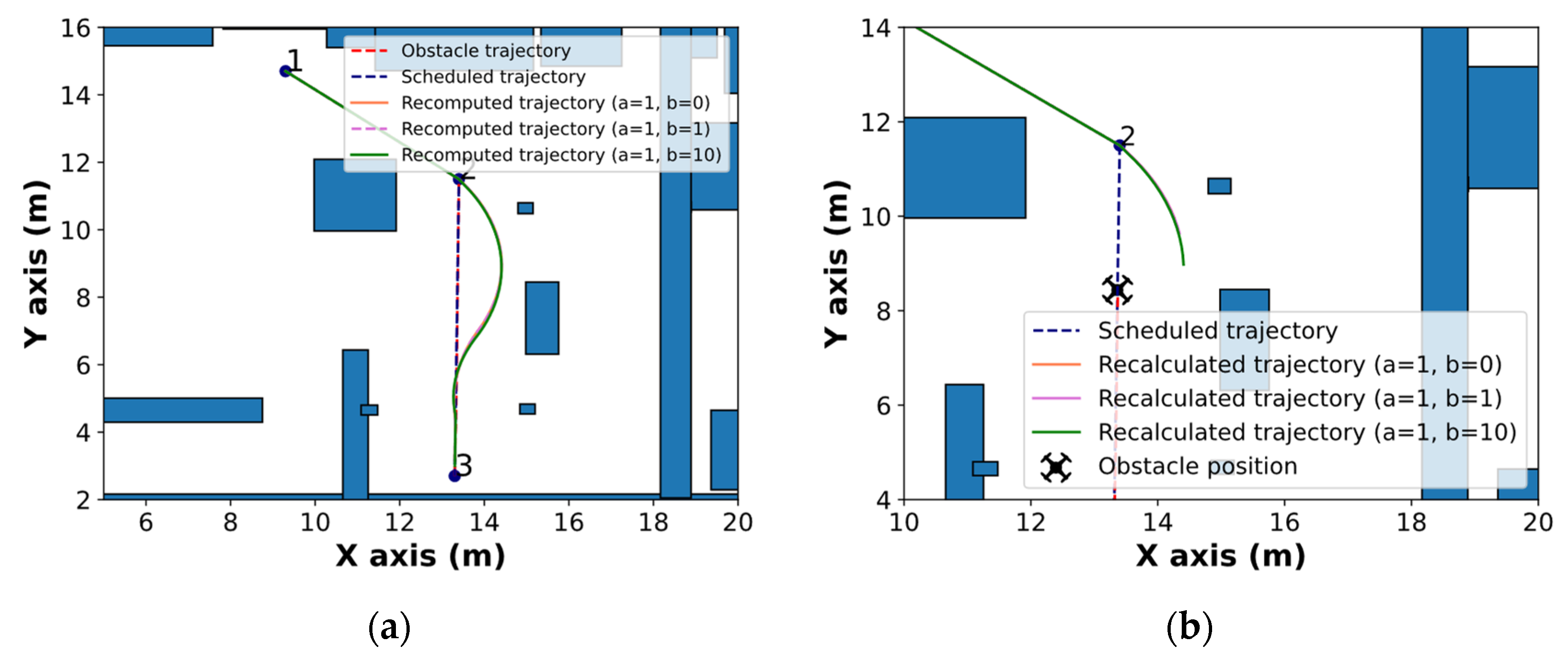
• Colinear moving obstacle: The obstacle moves in the opposite direction to the UAV at a constant speed of 1 m/s.
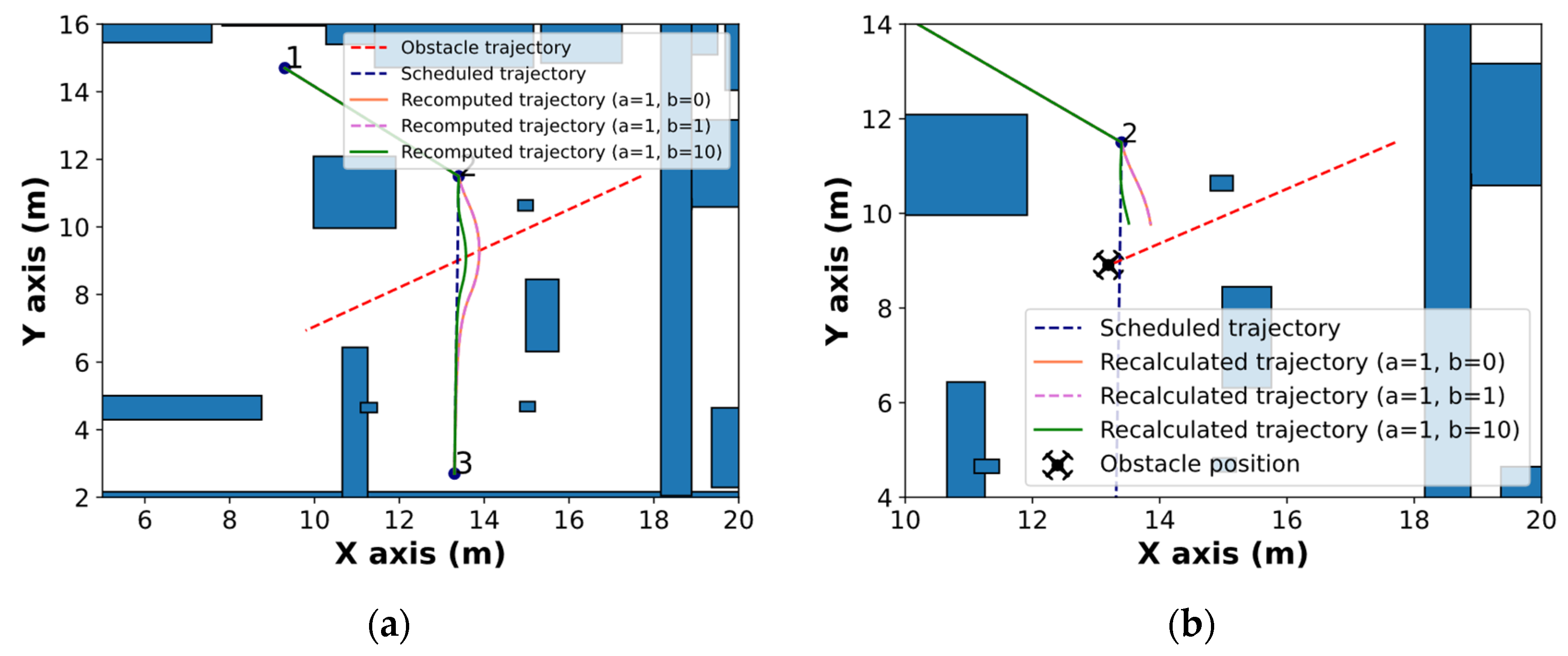
• Oblique moving obstacle: A similar scenario to the one presented in the previous cases, but with a different incidence angle.

Two additional cases were simulated in the MTI building to demonstrate other types of maneuvers such as vertical avoidance and obstacles following curved accelerated trajectories (Figure 8). In these test cases, the obstacle was detected between the first and second waypoint, and in an equivalent way as for the previous scenarios, the avoidance maneuver can be calculated:

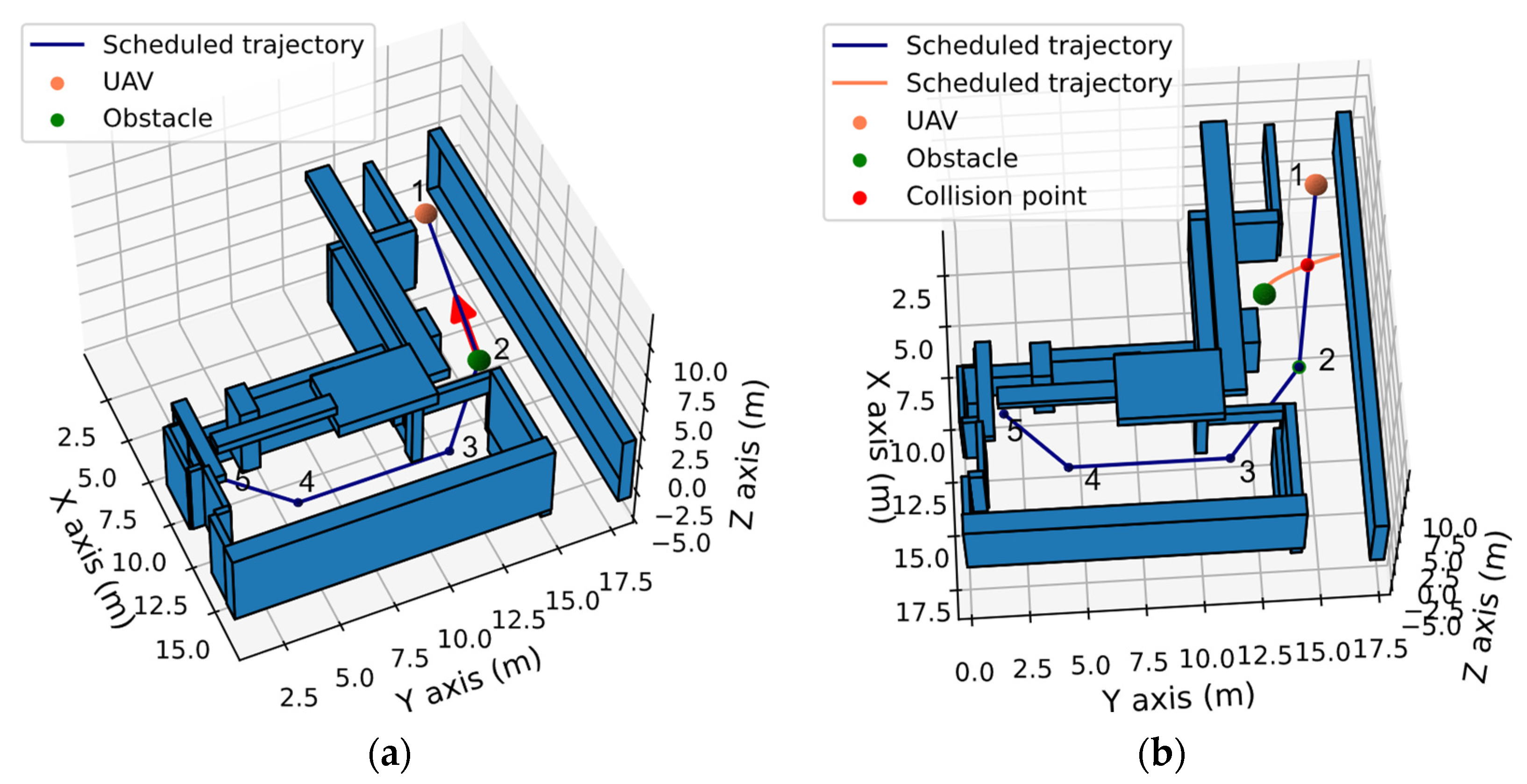
• Vertical avoidance: In this test case, a simple colinear obstacle is simulated. Vertical avoidance is a feasible maneuver as the height of the ceiling of the MTI building is around 5 m.
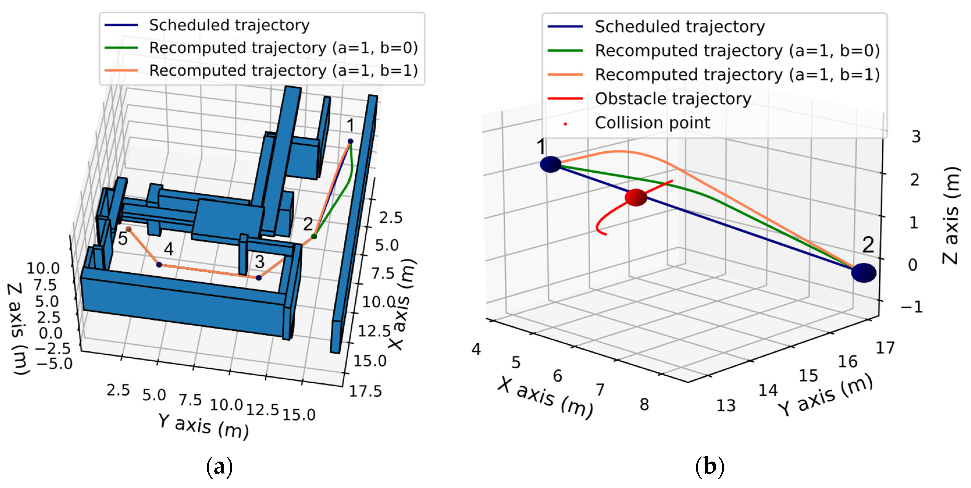
• Curved accelerated obstacle trajectory: An accelerated parabolic obstacle trajectory to demonstrate the capabilities of the proposed method to avoid obstacles with complex trajectories. The obstacle moves at a constant speed in the x direction and has a constant acceleration in the y component.

3.2. Avoidance Maneuvers

In this section, the results obtained from the application of the developed algorithm to the study cases introduced in the previous section are shown and analyzed.

3.2.1. Static Obstacle

Figure 9 depicts the recalculated path for the first test case scenario. As can be appreciated, between waypoints 1 and 2, the UAV deviated from the original path to avoid the obstacle. In this test case, the parametric study of parameters a and b was not performed as for static obstacles, with the fastest route being the shortest one.

3.2.2. Obstacle Moving Perpendicularly toward the UAV

Figure 10 represents the different approaches in this avoiding maneuver when using different settings of parameters a and b. For b equal to 0, the algorithm prioritizes the time of flight and creates a path at the maximum allowable speed of the UAV, for that, it takes a certain deviation from the original trajectory to maintain the safety distance from the obstacle. When increasing the value of b, the trajectory becomes straighter, and the UAV reduces its velocity and allows the other obstacle to cross the intersection. For larger values of b, the trajectory would practically be a straight line.

3.2.3. Obstacle following a Colinear Trajectory toward the UAV

In the third test case, the behavior of the different settings of the algorithm is practically the same as the obstacle is heading directly to the UAV. As depicted in Figure 11, the algorithm generates an arc to avoid the frontal collision with the moving obstacle.

3.2.4. Obstacle following an Oblique Trajectory toward the UAV

A similar behavior to Section 3.2.2 is shown in this test case. Higher values of b imply a straighter trajectory, whereas smaller ones maximize the flight speed of the UAV, as shown in Figure 12b, at the time in which the obstacle passes the intersection, the distance travelled is less for b equal to 10.

3.2.5. Vertical Avoidance

In this test, the same results were obtained for the different algorithm configurations. The UAV flew over the obstacle to maintain the safety distance, as shown in Figure 13.

3.2.6. Curved Accelerated Trajectory

For this last trajectory, different results were obtained depending on the algorithm configuration. If b equals 0, the UAV horizontally avoids the obstacle to decrease the flight time. By increasing the value of b, a vertical arc is obtained to minimize lateral deviation (Figure 14). Intermediate maneuvers could be obtained by properly setting the value of b.

3.3. Computation Time

Table 1. Time of computation (s).

Scenario	25 Discretization Points	50 Discretization Points	100 Discretization Points
Fixed obstacle	0.07	0.09	0.25
Perpendicular obstacle	0.08	0.13	0.42
Colinear obstacle	0.06	0.10	0.25
Oblique obstacle	0.08	0.11	0.38
Vertical avoidance	0.08	0.15	0.57
Curved accelerated obstacle trajectory	0.10	0.13	0.42

presents the calculation time of the maneuvers for different numbers of collocation points. All the computations were performed in a laptop using an AMD Ryzen 5 3500U processor. The calculation time may vary depending on the complexity of the maneuver, but generally quite satisfactory results were obtained using inexpensive equipment. In the case of 50 points, the average spacing between points in the evaluated maneuvers was less than 20 cm, a quite acceptable resolution for this type of trajectory. Judging by the results, the solution can be considered as a real time obstacle avoidance algorithm, since for 50 collocation points, the average calculation time was 0.118 s, so with a maximum movement speed of 1 m/s, the UAV will be displaced 11.8 cm. It is 10 times less than the security distance selected, that is 1 m. Given the calculation times, it would even be possible to recalculate the path if a deviation from the expected path of the moving obstacle is detected. The calculation time would be even less since the IPOPT algorithm would have a good initial guess value given by the previously calculated route.

The obtained computation times were considerably smaller than other conflict resolution algorithms based on optimal control. For instance, in [34], the computation time, according to the authors (using 50 discretization points for each aircraft) was 474 s and in [35], it was around 50 s. As aforementioned, the key objective of this work was to lighten up the algorithm as much as possible, and control inputs were not calculated as they did in previous works. Besides the problem, dimensionality was considerably reduced through logical evaluations, and the room obstacles were represented through a single constraint as explained in the Methodology section. These two factors were the main factors that allowed us to reduce computation time.

4. Conclusions

This article presents an obstacle avoidance algorithm developed for the autonomous navigation of UAVs in indoor building environments. The main aim of this work was to provide a methodology to avoid fixed and moving obstacles that were not considered in the trajectory planning, enabling these vehicles to perform autonomous missions in shared spaces with humans or other machinery.

The developed algorithm reached the following goals:

• The algorithm can avoid fixed and moving obstacles.
• The calculated trajectories are optimal in terms of deviation in time and position from the planned route.
• UAV performance limitations are considered in the obstacle avoidance protocols.
• Room model was successfully included in the avoidance algorithm.
• Computation times are affordable for real-time implementation.

In future works, this collision avoidance algorithm could be implemented in a Software in the Loop simulation. The dynamics of the UAV could be simulated as well as the motion of the obstacles. Besides, it is intended to introduce a real-time trajectory calculation program that allows correcting the UAV’s path if the detected obstacles modify its movement with respect to the estimated trajectory. In the current implementation, the main objective was to minimize the time of flight and deviation from the original trajectory. However, other objectives such as minimizing power consumption could be introduced in the objective function, and more elaboration can be conducted in future works from this aspect. Furthermore, another possibility could be extending the algorithm to control more than one UAV by introducing more control variables, representing the position of each drone. This possibility could be implemented to control a swarm of UAVs that would be typically operated for inspection tasks in a building environment. Additionally, the algorithm will be improved, making it run faster using parallel programming techniques.

References

- González-Jorge, H.; Martínez-Sánchez, J.; Bueno, M.; Arias, P. Unmanned aerial systems for civil applications: A review. Drones 2017, 1, 2. [Google Scholar] [CrossRef]
- Sony, S.; Laventure, S.; Sadhu, A. A literature review of next-generation smart sensing technology in structural health monitoring. Struct. Control Health Monit. 2019, 26, e2321. [Google Scholar] [CrossRef]
- Nex, F.; Remondino, F. UAV for 3D mapping applications: A review. Appl. Geomat. 2014, 6, 1–15. [Google Scholar] [CrossRef]
- Freeman, M.R.; Kashani, M.M.; Vardanega, P.J. Aerial robotic technologies for civil engineering: Established and emerging practice. J. Unmanned Veh. Syst. 2021, 9, 75–91. [Google Scholar] [CrossRef]
- Kim, K.; Kim, S.; Shchur, D. A UAS-based work zone safety monitoring system by integrating internal traffic control plan (ITCP) and automated object detection in game engine environment. Autom. Constr. 2021, 128, 103736. [Google Scholar] [CrossRef]
- Boukoberine, M.N.; Zhou, Z.; Benbouzid, M. A critical review on unmanned aerial vehicles power supply and energy management: Solutions, strategies, and prospects. Appl. Energy 2019, 255, 113823. [Google Scholar] [CrossRef]
- Elistair SAFE-T Tethered Drone Station. Available online: https://elistair.com/safe-t-tethered-drone-station/ (accessed on 5 October 2021).
- Rakha, T.; Gorodetsky, A. Review of Unmanned Aerial System (UAS) applications in the built environment: Towards automated building inspection procedures using drones. Autom. Constr. 2018, 93, 252–264. [Google Scholar] [CrossRef]
- Ekanayake, B.; Wong, J.K.W.; Fini, A.A.F.; Smith, P. Computer vision-based interior construction progress monitoring: A literature review and future research directions. Autom. Constr. 2021, 127, 103705. [Google Scholar] [CrossRef]
- Jiang, W.; Zhou, Y.; Ding, L.; Zhou, C.; Ning, X. UAV-based 3D reconstruction for hoist site mapping and layout planning in petrochemical construction. Autom. Constr. 2020, 113, 103137. [Google Scholar] [CrossRef]
- Wu, J.; Peng, L.; Li, J.; Zhou, X.; Zhong, J.; Wang, C.; Sun, J. Rapid safety monitoring and analysis of foundation pit construction using unmanned aerial vehicle images. Autom. Constr. 2021, 128, 103706. [Google Scholar] [CrossRef]
- Puri, N.; Turkan, Y. Bridge construction progress monitoring using lidar and 4D design models. Autom. Constr. 2020, 109, 102961. [Google Scholar] [CrossRef]
- Rebolj, D.; Pučko, Z.; Babič, N.Č.; Bizjak, M.; Mongus, D. Point cloud quality requirements for Scan-vs-BIM based automated construction progress monitoring. Autom. Constr. 2017, 84, 323–334. [Google Scholar] [CrossRef]
- Azimi, M.; Eslamlou, A.D.; Pekcan, G. Data-driven structural health monitoring and damage detection through deep learning: State-ofthe- art review. Sensors 2020, 20, 2778. [Google Scholar] [CrossRef]
- González-deSantos, L.M.; Martínez-Sánchez, J.; González-Jorge, H.; Navarro-Medina, F.; Arias, P. UAV payload with collision mitigation for contact inspection. Autom. Constr. 2020, 115, 103200. [Google Scholar] [CrossRef]
- Trujillo, M.; Martínez-de Dios, J.; Martín, C.; Viguria, A.; Ollero, A. Novel Aerial Manipulator for Accurate and Robust Industrial NDT Contact Inspection: A New Tool for the Oil and Gas Inspection Industry. Sensors 2019, 19, 1305. [Google Scholar] [CrossRef] [PubMed]
- Jeelani, I.; Gheisari, M. Safety challenges of UAV integration in construction: Conceptual analysis and future research roadmap. Saf. Sci. 2021, 144, 105473. [Google Scholar] [CrossRef]
- Guo, J.; Liang, C.; Wang, K.; Sang, B.; Wu, Y. Three-Dimensional Autonomous Obstacle Avoidance Algorithm for UAV Based on Circular Arc Trajectory. Int. J. Aerosp. Eng. 2021, 2021, 1–13. [Google Scholar] [CrossRef]
- Sasongko, R.A.; Rawikara, S.S.; Tampubolon, H.J. UAV Obstacle Avoidance Algorithm Based on Ellipsoid Geometry. J. Intell. Robot. Syst. Theory Appl. 2017, 88, 567–581. [Google Scholar] [CrossRef]
- Singh, R.; Bera, T.K. Obstacle Avoidance of Mobile Robot using Fuzzy Logic and Hybrid Obstacle Avoidance Algorithm. In Proceedings of the IOP Conference Series: Materials Science and Engineering; IOP Publishing: Bristol, UK, 2019; Volume 517. [Google Scholar]
- Khairudin, M.; Refalda, R.; Yatmono, S.; Pramono, H.S.; Triatmaja, A.K.; Shah, A. The mobile robot control in obstacle avoidance using fuzzy logic controller. Indones. J. Sci. Technol. 2020, 5, 334–351. [Google Scholar] [CrossRef]
- Cetin, O.; Zagli, I.; Yilmaz, G. Establishing obstacle and collision free communication relay for UAVs with artificial potential fields. J. Intell. Robot. Syst. Theory Appl. 2013, 69, 361–372. [Google Scholar] [CrossRef]
- Fan, X.; Guo, Y.; Liu, H.; Wei, B.; Lyu, W. Improved Artificial Potential Field Method Applied for AUV Path Planning. Math. Probl. Eng. 2020, 2020, 1–21. [Google Scholar] [CrossRef]
- Zhang, T.; Kahn, G.; Levine, S.; Abbeel, P. Learning deep control policies for autonomous aerial vehicles with MPC-guided policy search. In Proceedings of the IEEE International Conference on Robotics and Automation, Stockholm, Sweden, 16–21 May 2016; Volume 2016. [Google Scholar]
- Han, X.; Wang, J.; Xue, J.; Zhang, Q. Intelligent Decision-Making for 3-Dimensional Dynamic Obstacle Avoidance of UAV Based on Deep Reinforcement Learning. In Proceedings of the 2019 11th International Conference on Wireless Communications and Signal Processing, WCSP 2019, Xi’an, China, 23–25 October 2019. [Google Scholar]
- Dai, X.; Mao, Y.; Huang, T.; Qin, N.; Huang, D.; Li, Y. Automatic obstacle avoidance of quadrotor UAV via CNN-based learning. Neurocomputing 2020, 402, 346–358. [Google Scholar] [CrossRef]
- Xin, C.; Wu, G.; Zhang, C.; Chen, K.; Wang, J.; Wang, X. Research on indoor navigation system of uav based on lidar. In Proceedings of the 2020 12th International Conference on Measuring Technology and Mechatronics Automation (ICMTMA), Phuket, Thailand, 28–29 February 2020; pp. 763–766. [Google Scholar]
- Ajay Kumar, G.; Patil, A.K.; Patil, R.; Park, S.S.; Chai, Y.H. A LiDAR and IMU integrated indoor navigation system for UAVs and its application in real-time pipeline classification. Sensors 2017, 17, 1268. [Google Scholar] [CrossRef]
- Mane, S.B.; Vhanale, S. Real time obstacle detection for mobile robot navigation using stereo vision. In Proceedings of the International Conference on Computing, Analytics and Security Trends, CAST 2016, Pune, India, 19–21 December 2016. [Google Scholar]
- Di Lizia, P.; Armellin, R.; Bernelli-Zazzera, F.; Berz, M. High order optimal control of space trajectories with uncertain boundary conditions. Acta Astronaut. 2014, 93, 217–229. [Google Scholar] [CrossRef]
- Chu, H.; Ma, L.; Wang, K.; Shao, Z.; Song, Z. Trajectory optimization for lunar soft landing with complex constraints. Adv. Space Res. 2017, 60, 2060–2076. [Google Scholar] [CrossRef]
- Chai, R.; Savvaris, A.; Tsourdos, A.; Chai, S.; Xia, Y. Trajectory Optimization of Space Maneuver Vehicle Using a Hybrid Optimal Control Solver. IEEE Trans. Cybern. 2019, 49, 467–480. [Google Scholar] [CrossRef]
- Olympio, J.T. A Continuous Implementation of a Second-Variation Optimal Control Method for Space Trajectory Problems. J. Optim. Theory Appl. 2013, 158, 687–716. [Google Scholar] [CrossRef]
- Soler, M.; Kamgarpour, M.; Lloret, J.; Lygeros, J. A Hybrid Optimal Control Approach to Fuel-Efficient Aircraft Conflict Avoidance. IEEE Trans. Intell. Transp. Syst. 2016, 17, 1826–1838. [Google Scholar] [CrossRef]
- Cai, J.; Zhang, N. Mixed Integer Nonlinear Programming for Aircraft Conflict Avoidance by Applying Velocity and Altitude Changes. Arab. J. Sci. Eng. 2019, 44, 8893–8903. [Google Scholar] [CrossRef]
- Cai, J.; Zhang, N. Mixed integer nonlinear programming for three-dimensional aircraft conflict avoidance. PeerJ 2018, 6, e27410v1. [Google Scholar] [CrossRef][Green Version]
- Petit, M.L. Dynamic optimization. The calculus of variations and optimal control in economics and management. Int. Rev. Econ. Financ. 1994, 3, 245–247. [Google Scholar] [CrossRef]
- Augeraud-Véron, E.; Boucekkine, R.; Veliov, V.M. Distributed optimal control models in environmental economics: A review. Math. Model. Nat. Phenom. 2019, 14, 106. [Google Scholar] [CrossRef]
- Karush, W. Minima of functions of several variables with inequalities as side conditions. In Traces and Emergence of Nonlinear Programming; Springer: New York, NY, USA, 2014. [Google Scholar]
- Wächter, A.; Biegler, L.T. On the implementation of an interior-point filter line-search algorithm for large-scale nonlinear programming. Math. Program. 2006, 106, 25–27. [Google Scholar] [CrossRef]
- González-Desantos, L.M.; Frías, E.; Martínez-Sánchez, J.; González-Jorge, H. Indoor path-planning algorithm for uav-based contact inspection. Sensors 2021, 21, 642. [Google Scholar] [CrossRef] [PubMed]
- Hart, P.E.; Nilsson, N.J.; Raphael, B. A Formal Basis for the Heuristic Determination of Minimum Cost Paths. IEEE Trans. Syst. Sci. Cybern. 1968, 4, 100–107. [Google Scholar] [CrossRef]
- GeoSLAM Ltd. ZEB-REVO Laser Scanner. Available online: https://download.geoslam.com/docs/zeb-revo/ZEB-REVOUserGuideV3.0.0.pdf (accessed on 3 November 2020).
- FARO, Inc. Faro Focus 3D X330. Available online: https://downloads.faro.com/index.php/s/z6nEwtBPDpGPmYW?dir=undefined&openfile=42057 (accessed on 27 August 2021).