1. Introduction
Searching missions started to gain value in the maritime field during World War II, when the US Army tried to detect enemy submarines. Currently, these exploration tasks have received a great amount of attention for different reasons, focused on civilian applications. Current efforts target search and rescue missions of passengers affected by a maritime accident and the search for wreckage scattered across the ocean. Search operations on the ocean surface remain a complex task due to the dynamics of the wind and ocean currents, spreading lost targets and debris in an unpredictable way. A remarkable real scenario that inspired this field of research is the search for Malaysian Flight 370 (MH370). The aircraft disappeared in the middle of the ocean midflight in March 2014, after takeoff from Kuala Lumpur on its way to Beijing carrying 239 people. The search operations covered an area of over 4,600,000 km
in the Indian Ocean and involved a total of 40 ships and aircrafts. The search did not yield any evidence and was consequently canceled [
1].
Numerous researchers have used the MH730 case to develop algorithms capable of tracking and finding lost debris from wreckages. Miron [
2] et al. used a method based on Markov chains. They developed a framework that uses the locations and times of confirmed airplane debris beachings and historical trajectories produced by drifters to restrict the location of the crash site. García-Garrido [
3] et al. proposed the use of Lagrangian descriptors in combination with publicly available ocean data sources to assess the spatiotemporal state of the ocean in the priority search area at the time of impact and the following weeks. Trinanes [
4] et al. also used data sets of surface drifters to backtrack ocean debris based on the location where it was found that provides information on the potential crash site.
Some more recent approaches such as that of [
5] use a team of UAVs with MIMO radars to estimate the direction of arrival of the target ships by reconstructing the support of a block sparse matrix. The disadvantage is that a ship with a GPS signal needs to be deployed to know the UAVs and targets positions. The appropach proposed by Xiao et al. [
6] uses UAVs to help in marine mass casualty incident search and rescue by providing additional information to an USV operator. This method requires one operator for the USV and another one for the UAV.
Several approaches treat the search problem from different scopes, such as computer vision [
7,
8], wireless sensor network design [
9,
10], task allocation formulations [
11,
12], iterative optimization algorithms [
13], and optimal path planning calculations for autonomous vehicles to help in the search [
14,
15]. In this work, we aim at the latter, proposing an algorithm capable of providing the route for the vehicles to follow.
There are two main characteristics that define the design process of a search mission, mainly concerning the maritime field application [
16]:
Definition of the target area. Since the weather conditions in maritime environments are usually inaccurate or unknown and the air and ocean currents can drift the debris away from their last known position, it is necessary to establish a method to define the search target area.
Design of a search path. Even if the target area is correctly defined, there is no optimal solution for the design of the search trajectory problem. In this work, the goal is to compute paths along the whole searching area that cover the points with the higher probability of containment as fast as possible.
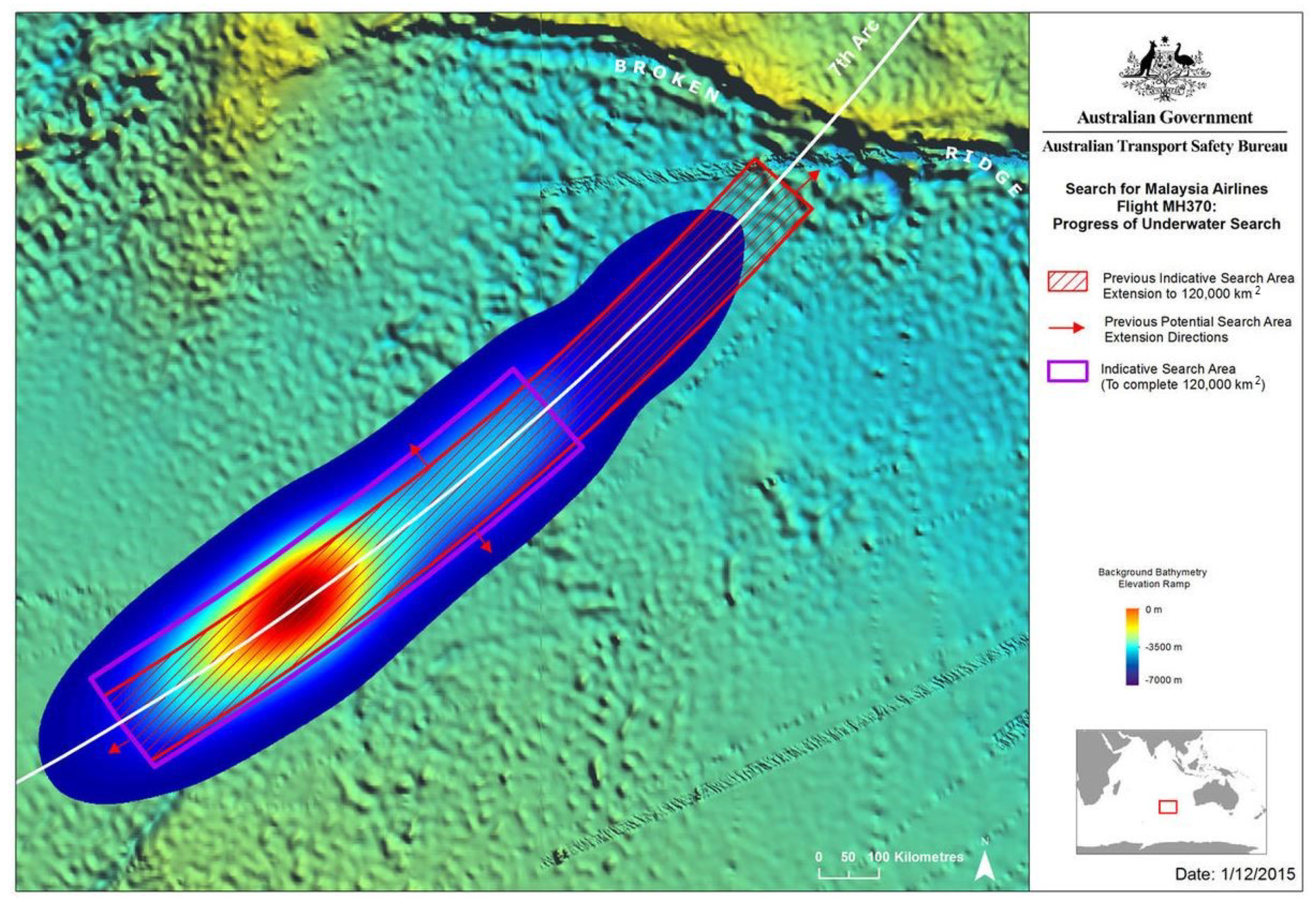
Regarding the establishment of the target area, the probability of containment is the first factor to be determined. This measure is defined as the probability to find the target in each specific region of the search area. Following this methodology, the search area is decomposed into cells and then turned into a probability map by assigning these partitions the probability value related to the chances of finding the search target. The resulting map will represent the possible positions of the targets, considering the ocean and wind currents. An example can be seen in
Figure 1, in which zones with lower and higher probability of containment indices are distinguished through a color code. From that target position, a probability of containment map is calculated by deploying drifter particles around the target that follow the marine and wind currents and fitting them to a Gaussian probability distribution.
In this paper, we propose a target position estimation method and a coverage path planning algorithm for fixed-wing UAVs based on drifter particles and the differential evolution method. The proposed method has a great amount of potential in real world applications since the movement of the particles representing the possible positions of the lost target is based on real world current data from the OSCAR data set. Furthermore, a large number of particles is used to ensure a good representation of the lost target movement, as well as some noise applied to the OSCAR data to generate more possible outcomes for the drifter particles.
This work is aimed for fixed-wing UAVs based on the fact that they achieve greater speeds and have a greater autonomy, which is of great importance when tackling a marine search and rescue problem. They are also more wind-resistant, can carry heavier payloads, which can help in the search and rescue missions, have greater stability, and can recover more easily from sudden power loss, which is important in marine environments. Moreover, they can achieve greater altitudes; when they are equipped with a long-range radar or camera, they can greatly improve the chances of target location. Fixed-wing UAVs are also better than multirotor UAVs when performing linear flights that, when considering the dimensions of the map and the length of each band, are going to be applied to our particular problem.
The use of UAVs is key in situations such as the one presented in this work, where there has been an accident or the target is missing, and it is necessary to perform a fast search. UAVs have a great advantage over USVs, since they have a better line of sight and can detect targets from afar. Furthermore, the depth perception from a USV is difficult, since objects may be far apart even though they appear close, and it is an even harder task when there are high and strong waves. These complications dissapear when using UAVs due to the fact that they have a clear top view from the sky and their depth perception is not affected. Since the results in this work focus on obtaining the coverage path and no real UAVs have been used, no UAV-specific characteristics have been taken into account. However, the coverage bandwidth and the desired height of the coverage path can be defined, making the algorithm able to adapt to any fixed-wing UAV.
Note that in the context of real world applications, UAVs need a ground base station and a piece of terrain to take off and land. Furthermore, the ground station needs to be within range of the target area for the coverage mission such that the UAV meets the necessary energy constraints to perform the mission and come back safely. Some applications use an aircraft carrier to carry the UAVs and act as the base station.
The differential evolution method is used to optimize the coverage angle for the search task, based on the probability of containment (POC) of each cell of the probability map, created from a Gaussian probability distribution generated from the positions of the drifter particles. Global optimization algorithms are necessary in fields such as engineering, statistics, and finance. However, many of these practical problems have objective functions that are nondifferentiable, noncontinuous, noisy, multidimensional, or have many local minima and constraints. These problems are difficult to solve analytically, so algorithms such as differential evolution can be used to find approximate solutions. The DE algorithm is the one used in this work since it has proved useful in previous publications, but any optimization algorithm with similar characteristics could be used.
The rest of the paper is organized as follows. Section II describes the methodology used for the target position estimation and introduces the coverage path planning method. Section III presents the results of the simulations performed to test the algorithm. Finally, in section IV, the main conclusions of the work are outlined.
2. Materials and Methods
This section details both the target position estimation of the target method and the coverage path planning algorithm used to search for the target. The target estimation of the target position is performed by dropping drifter particles that move with the ocean and wind currents and then fitting them to a Gaussian probability distribution to obtain the probability of containment map. The coverage path planning algorithm uses the differential evolution method to obtain the best coverage angle to cover the maximum probability of containment possible and then performs back-and-forth motions to create a coverage path.
2.1. Target Position Estimation
For the target position estimation process, the Ocean Surface Current Analysis (OSCAR) database [
17] is used to obtain an ocean current map. Once the map of the particular section of the wreckage is obtained from the database, a number of drifters are dropped around the target’s last known position within a determined radius. This method of drifters tracking to estimate the direction of ocean currents has been used for the generation of data sets such as [
18].
Once the drifters are placed on the map, they move following the currents given by the OSCAR database and some noise implemented due to variations in ocean drift and wind currents. The equation for calculating the next position of the particles is shown in Equation (
1):
where
is the next estimated position of the particles,
is the current estimated position of the particles,
is the velocity vector for the
x and
y axes,
is the maximum possible error in the ocean current velocity vector, and
is a random number in the interval [0,1]. In this case,
is calculated as
.
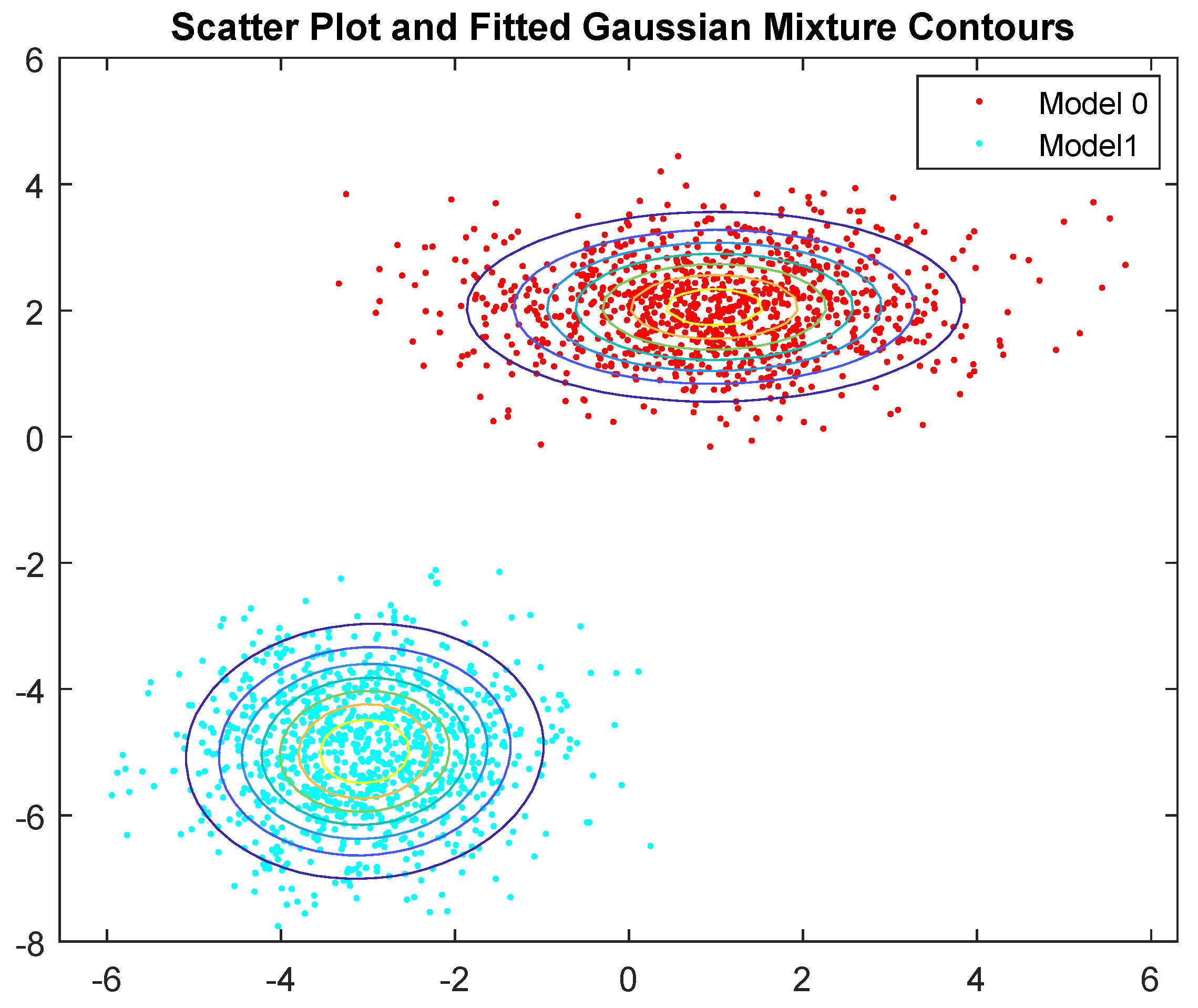
When the search is about to start, the particle distribution is fitted to a Gaussian mixture model [
19], which allows to gather all possible observations under a group of normal distributions of different parameters, as shown in
Figure 2.
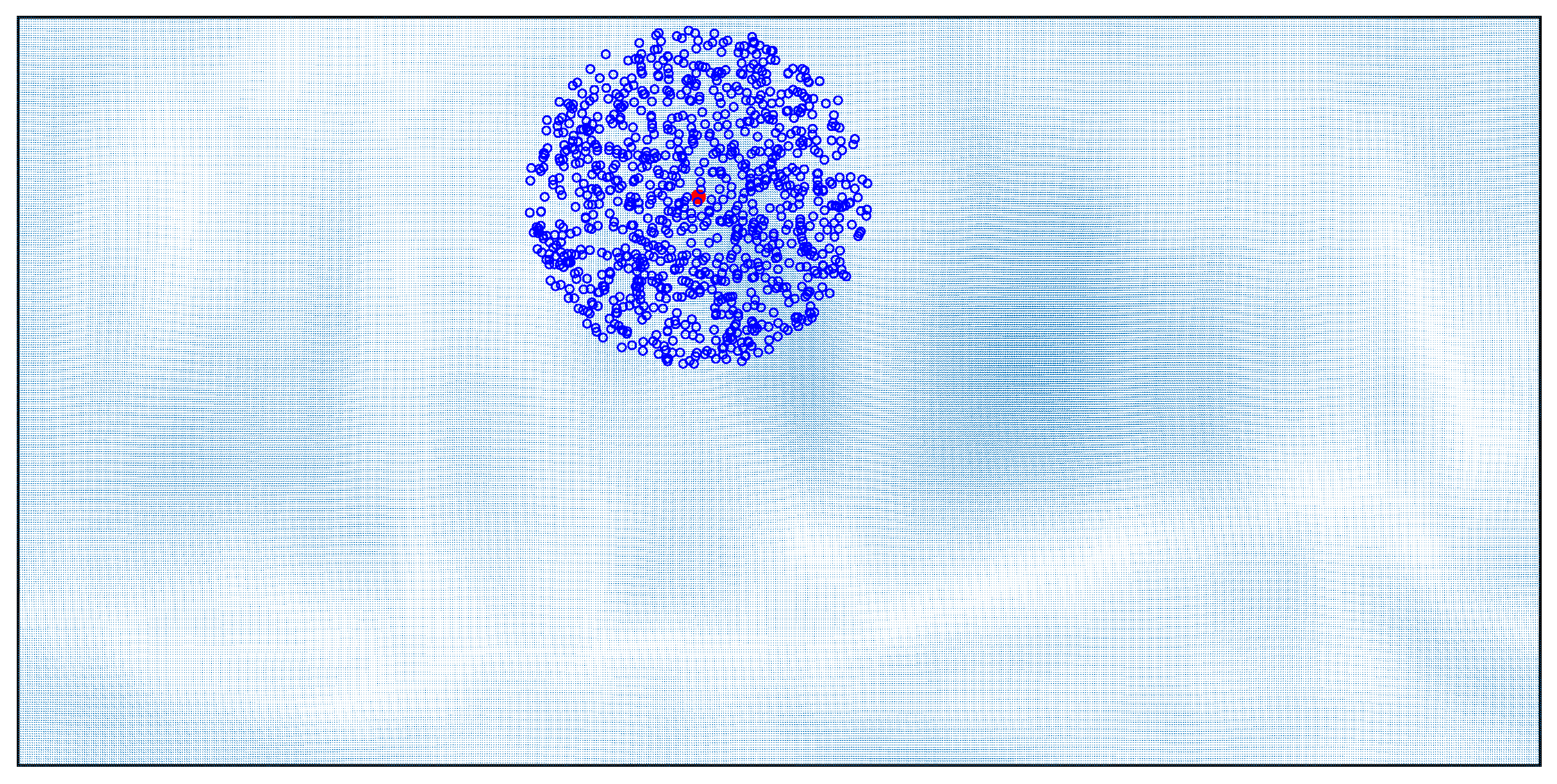
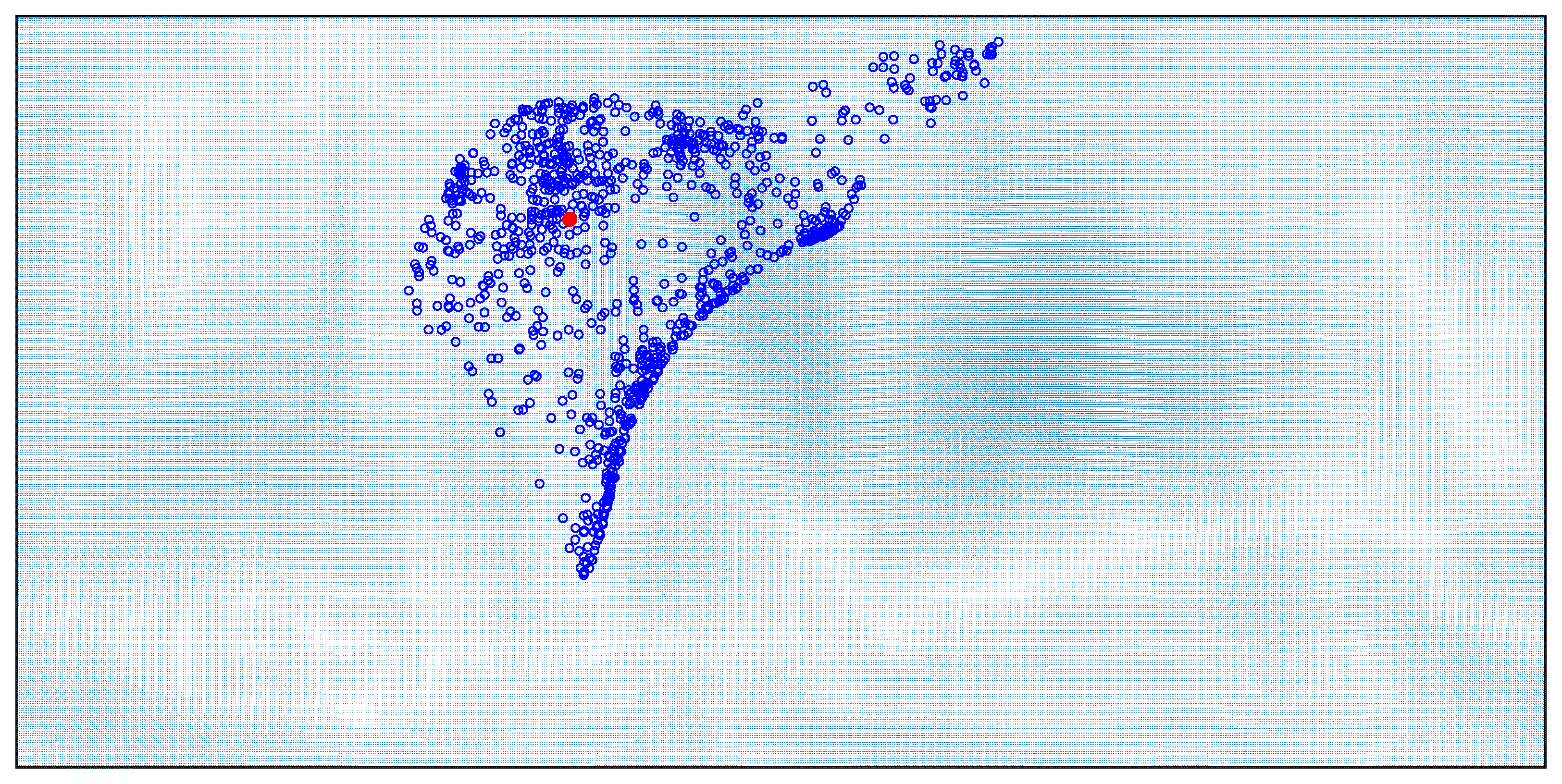
The first step is to drop the drifter particles around the target’s last known position. An example of initial drifter particles distribution is shown in
Figure 3. The red dot indicates the target’s last known position, and the blue dots are the drifter particles scattered around that position.
Once the drifters are distributed in a circular area around the target’s last known position, they start moving with the ocean and wind drift currents for the predefined duration, following Equation (
1). After the desired number of iterations have passed, the drifter particles positions are saved. The final positions of the drifter particles for the currents and particle distribution used above are shown in
Figure 4.
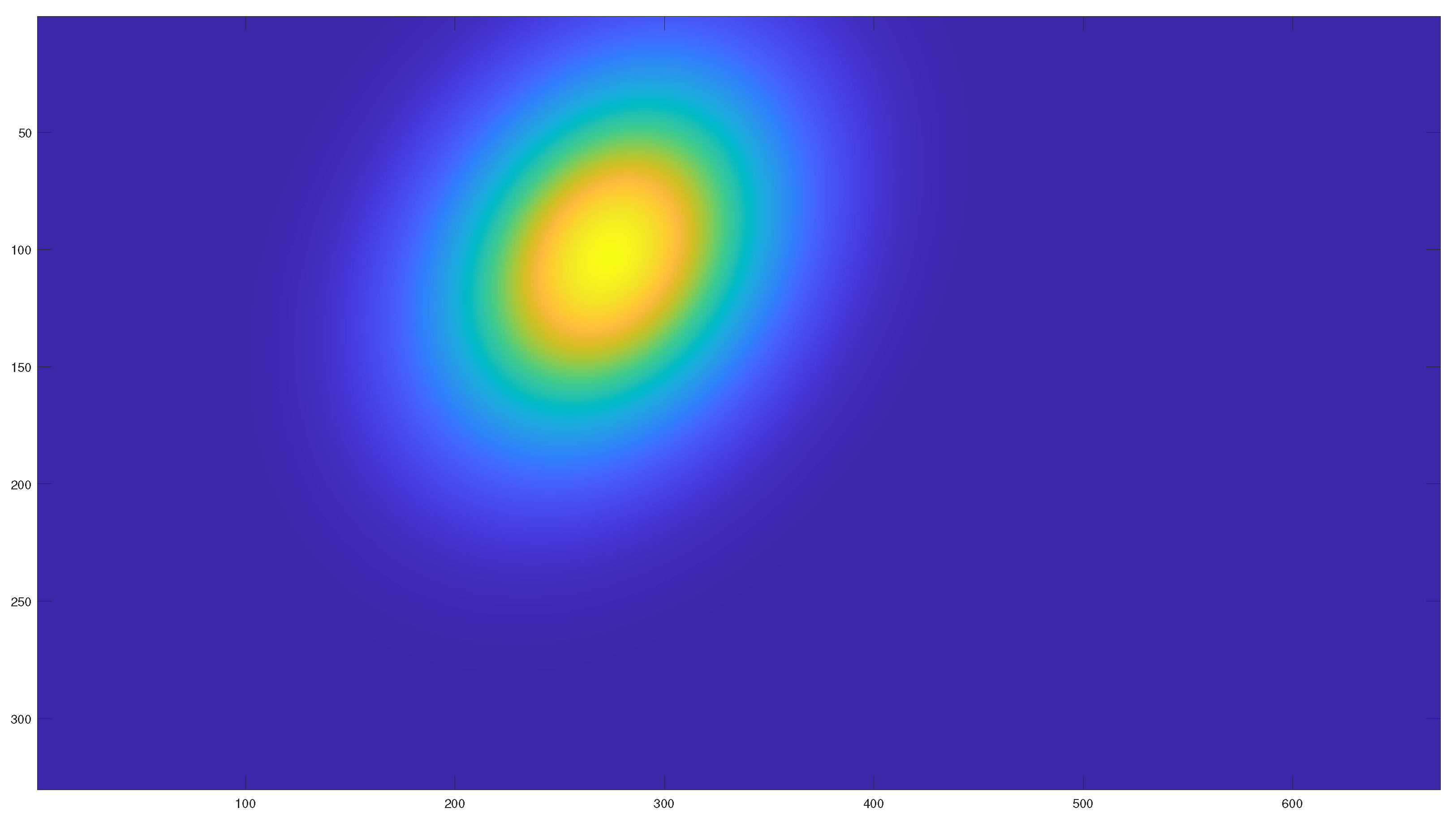
When the final positions of the drifter particles are saved, they are fitted to a Gaussian probability distribution, creating the probability of containment map. This probability of containment map obtained from the position of the drifter particles can be seen in
Figure 5. The cells with the highest probability of containment are shown in yellow, while the cells with low to zero probability of containment are shown in dark blue.
After the target position estimation process has been described, the following subsection focuses on obtaining the coverage path to maximize the probability of containment covered by the fixed-wing UAV.
2.2. Coverage Path Planning Algorithm
The coverage path planning algorithm used in this work is based on the differential evolution method. The differential evolution method is an evolutive filter designed to solve global optimization problems over continuous spaces, proposed by Storn and Price [
21].
The evolutive filter uses a direct parallel search method that uses parameter vectors of n dimensions to point each candidate solution i to the optimization problem in each iteration step k. This method uses N parameter vectors as a population for every generation t of the optimization process.
The initial population is chosen arbitrarily to uniformly cover the whole parameter space. In the absence of a priori information, the whole parameter space has the same probability to contain the optimal parameter vector and a uniform probability distribution is assumed.
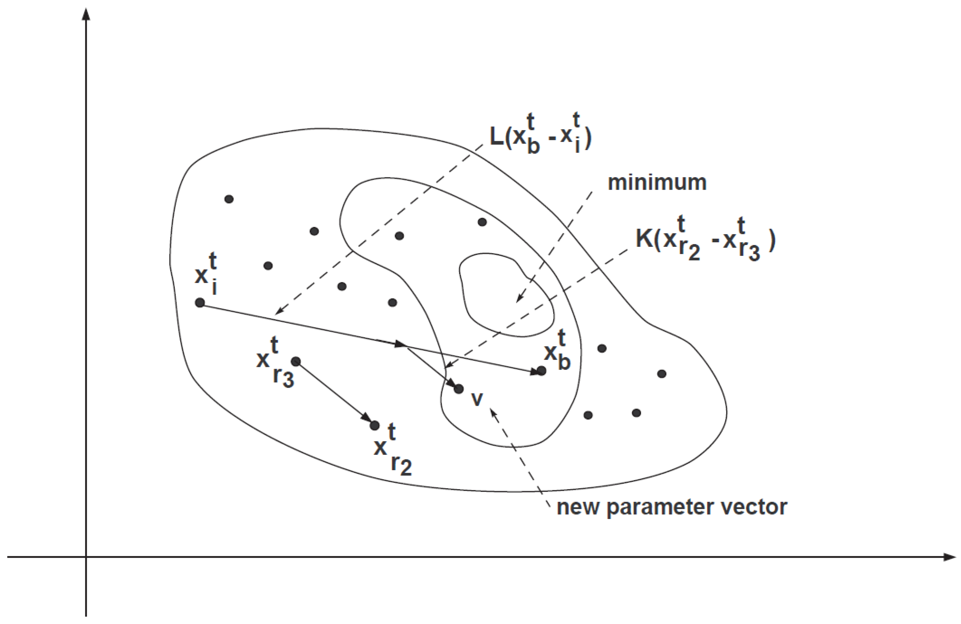
The evolutive filter generates new parameter vectors by adding the weighted difference vector between two population members to a third member, as it can be seen in
Figure 6. If the resulting vector yields a lower objective function value than the corresponding member of the previous population, the newly generated vector replaces the one which with it was compared; otherwise, the old vector is conserved.
This basic idea is extended by perturbing an existing vector through the addition of one or more weighed difference vectors. This perturbation scheme generates a variation
v according to the following equation:
where
is the parameter vector to be perturbed in iteration
k,
is the best parameter vector of the population in iteration
k, and
and
are the parameter vectors randomly chosen from the rest of the population.
L and
F are real and constant factors that control the amplification of the differential variables
and
.
With the purpose of incrementing the diversity of the new parameter vector generation, the crossover concept is introduced. We denote the new parameter vector by
with
where
is the exchanged parameter in member
,
is a random value in the interval
for each parameter
j of the population member
i in step
k, and
is the crossover probability and constitutes the crossover control variable. Random values
are created for each trial vector
i.
To decide whether or not vector should become a member of generation , the new vector is compared to . If vector yields a better value of the objective function than , then is replaced by ; on the contrary, the old value is saved for the next generation. Mutation, crossover, and selection mechanisms are well known and can be found in the literature.
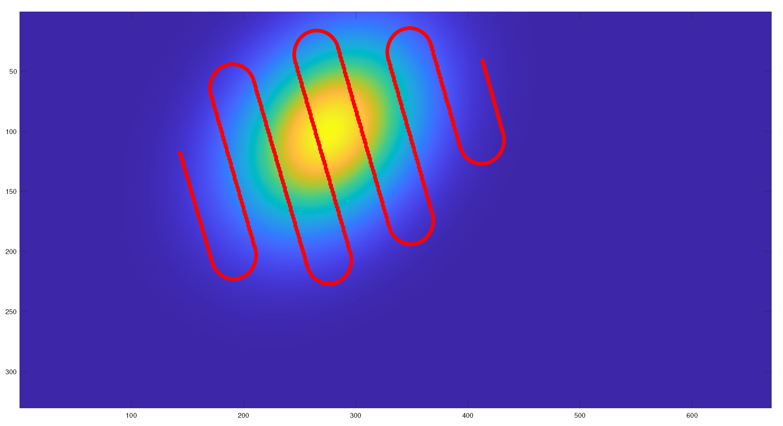
In order to calculate the coverage path, a binary mask is created by thresholding the POC (probability of containment) map. All cells with a POC value higher than a certain limit are considered into the coverage area. An example of a coverage binary mask is shown in
Figure 7. Then, the initial population is created with angles ranging from −90 to 90 degrees. For every member of the population, the coverage path is calculated with the given angle.
To test these angles, coverage bands are drawn perpendicular to the coverage angle direction. Then, all the bands that do not have enough points inside the coverage area are deleted. Afterward, the bands inside the coverage area are cut so that they keep a distance equal to the coverage bandwidth from the borders of the coverage area. Once the DE optimization process is finished and the final coverage angle is obtained, the path is calculated as explained before, but this time, the bands are linked with arcs to create a feasible path.
The cost function used with the differential evolution method to calculate the optimal coverage angle is shown in Equation (
2). All calculated paths are downsampled to 1000 waypoints, so the comparison between paths is fair. Furthermore, the cost function is applied twice to every path, starting from the first and last waypoints:
where
is the probability of containment cell map,
i is the path waypoints index, and
is the path calculated given a certain coverage angle.
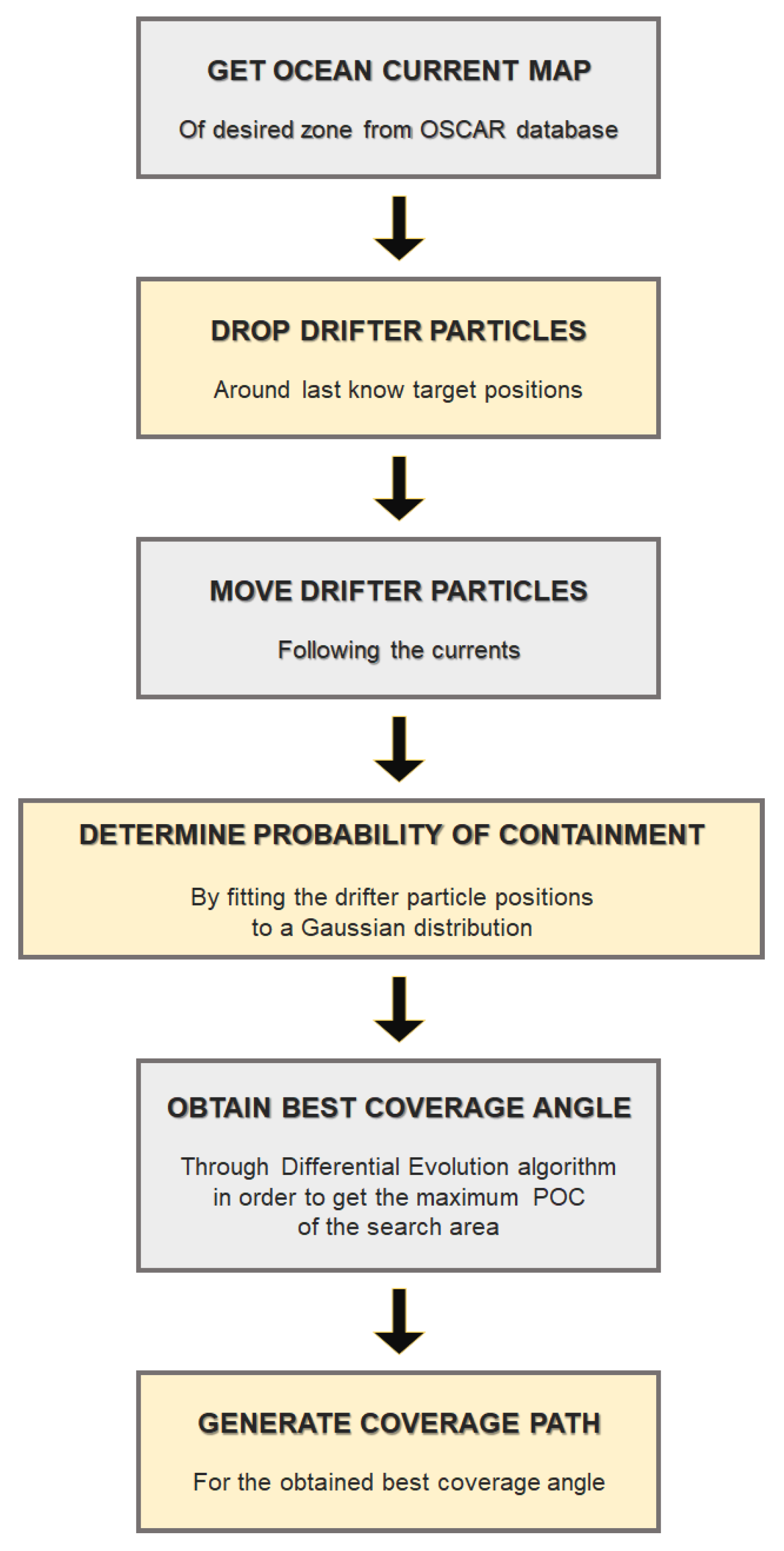
To better show the process followed by the proposed algorithm, a flowchart is shown in
Figure 8.
3. Results
Since we did not have access to a real fixed-wing UAV nor did we meet the necessary regulations to operate one, the tests were performed in a simulated environment in MATLAB. To test the effectiveness of the proposed algorithm, the coverage path planning simulation was run for a different number of parameters of the DE algorithm. The machine used to run the test was a computer with 16 GB RAM and an AMD Ryzen 5 5600X CPU @4.12 GHz. The first test was run for a fixed number of five members of the population and a number of iterations varying from 5 to 50. The measures collected from the tests were the total probability of containment based on the position of the waypoints of the obtained coverage path over the probability of containment distribution map, the total execution time taken by the algorithm to generate the coverage path, and the final angle obtained from the differential evolution algorithm when the iterations finished. Since the differential evolution algorithm has a stochastic nature, the measures for both the mean and the standard deviation (std) were collected. Results from this test can be seen in
Table 1:
The second test was run for a fixed number of 5 iterations, and a number of members of the population ranging from 5 to 50. Results from this test can be seen in
Table 2:
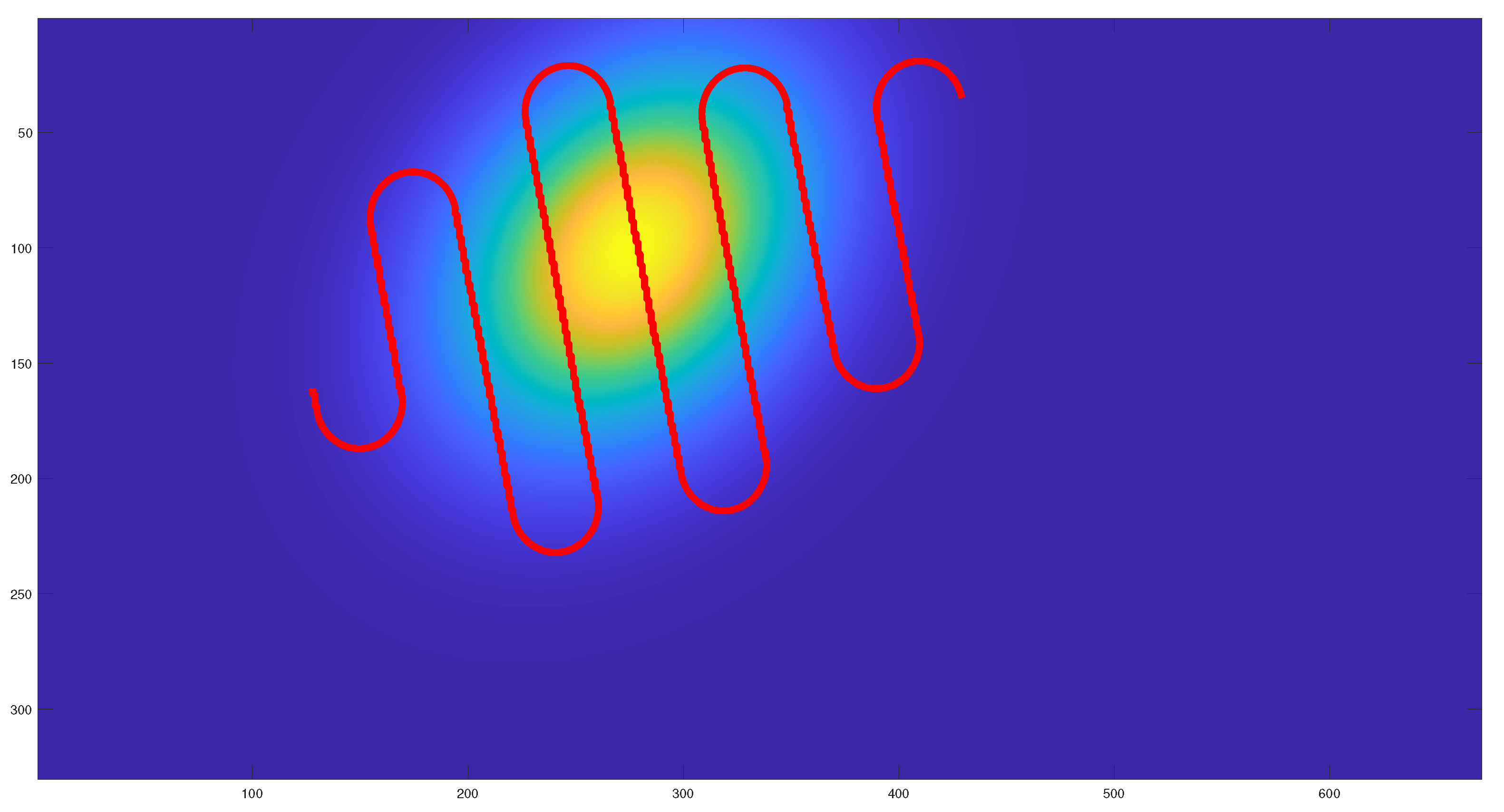
The tables show that after a determined number of iterations and members of the population, the obtained angle converges to a similar value, which we can consider as the near optimal coverage angle. This result is better reflected in
Figure 9,
Figure 10 and
Figure 11, where the initial and final paths obtained are similar.
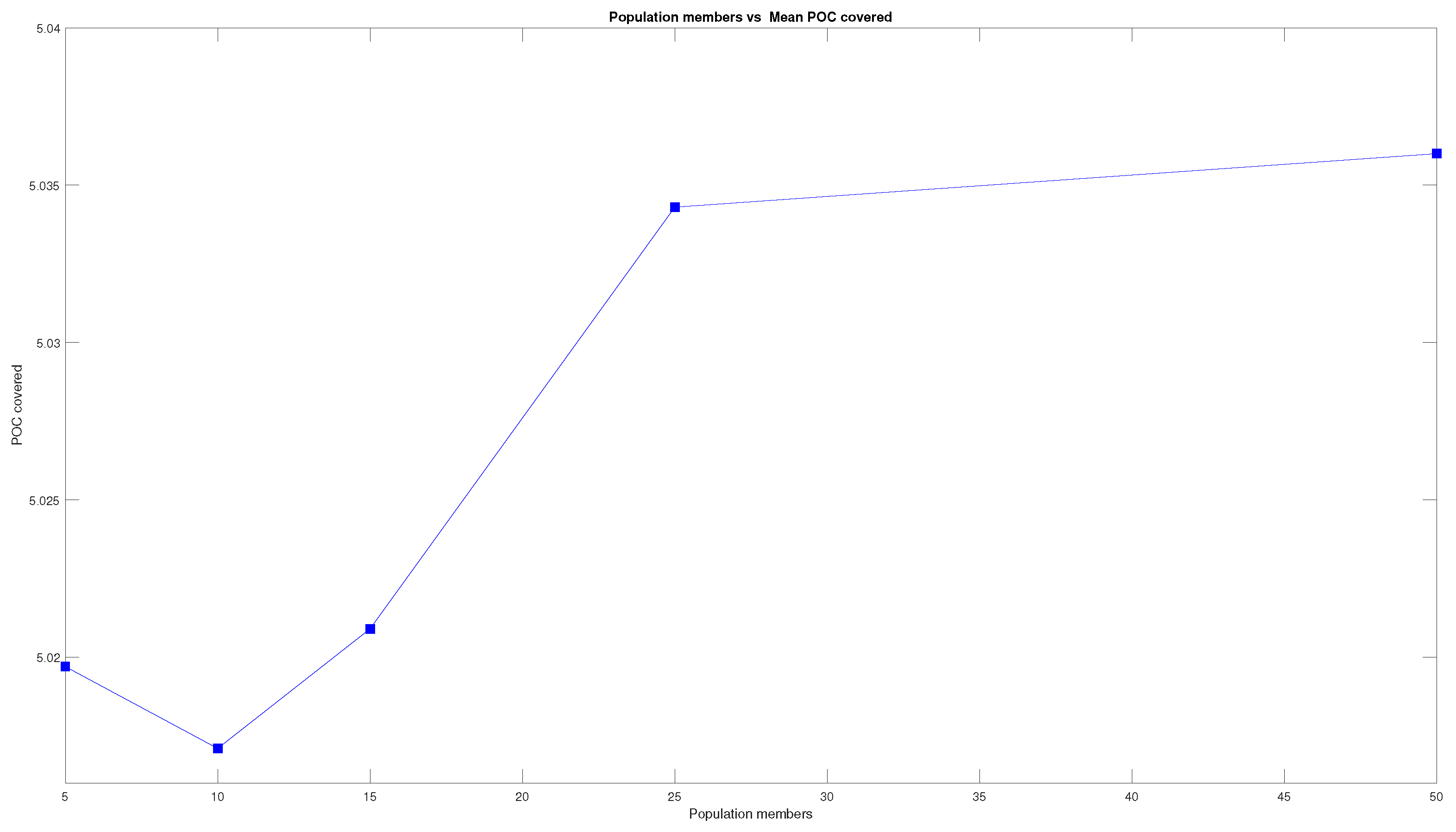
To better study the evolution of the POC as the number of iterations and members of the population increase, the results are plotted in graphs that can be seen in
Figure 12 and
Figure 13.
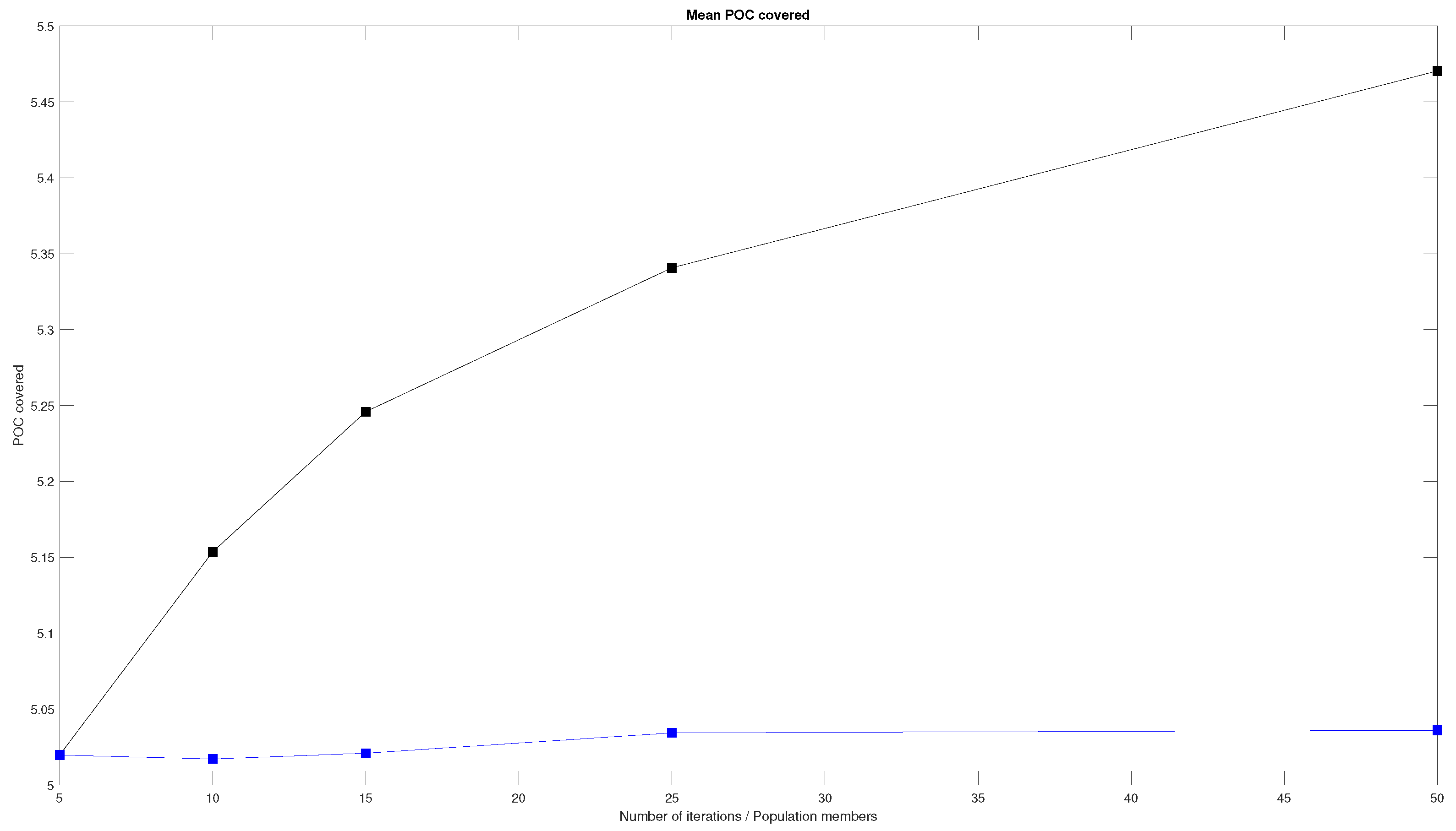
The Figures show that the mean POC increases with an increment in the number of iterations and members of the population. However, the increase is not the same in both cases. To better address this difference between the two parameters, the two graphs are plotted together in
Figure 14. The graph shows that the increase in the mean POC covered increases more greatly when adding more iterations than when adding more members of the population.
The above graphs show that, as a general rule, the results obtained from the DE algorithm improve as the number of members of the population and the number of iterations increase, but this increment becomes smaller as the DE algorithm gets closer to the optimal solution.
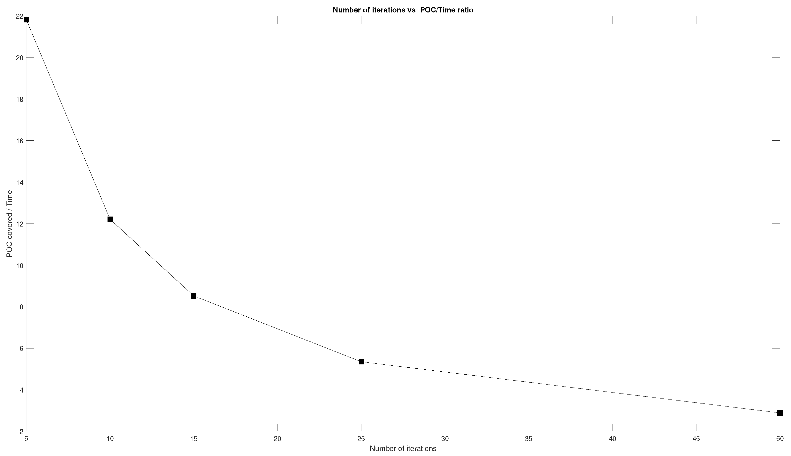
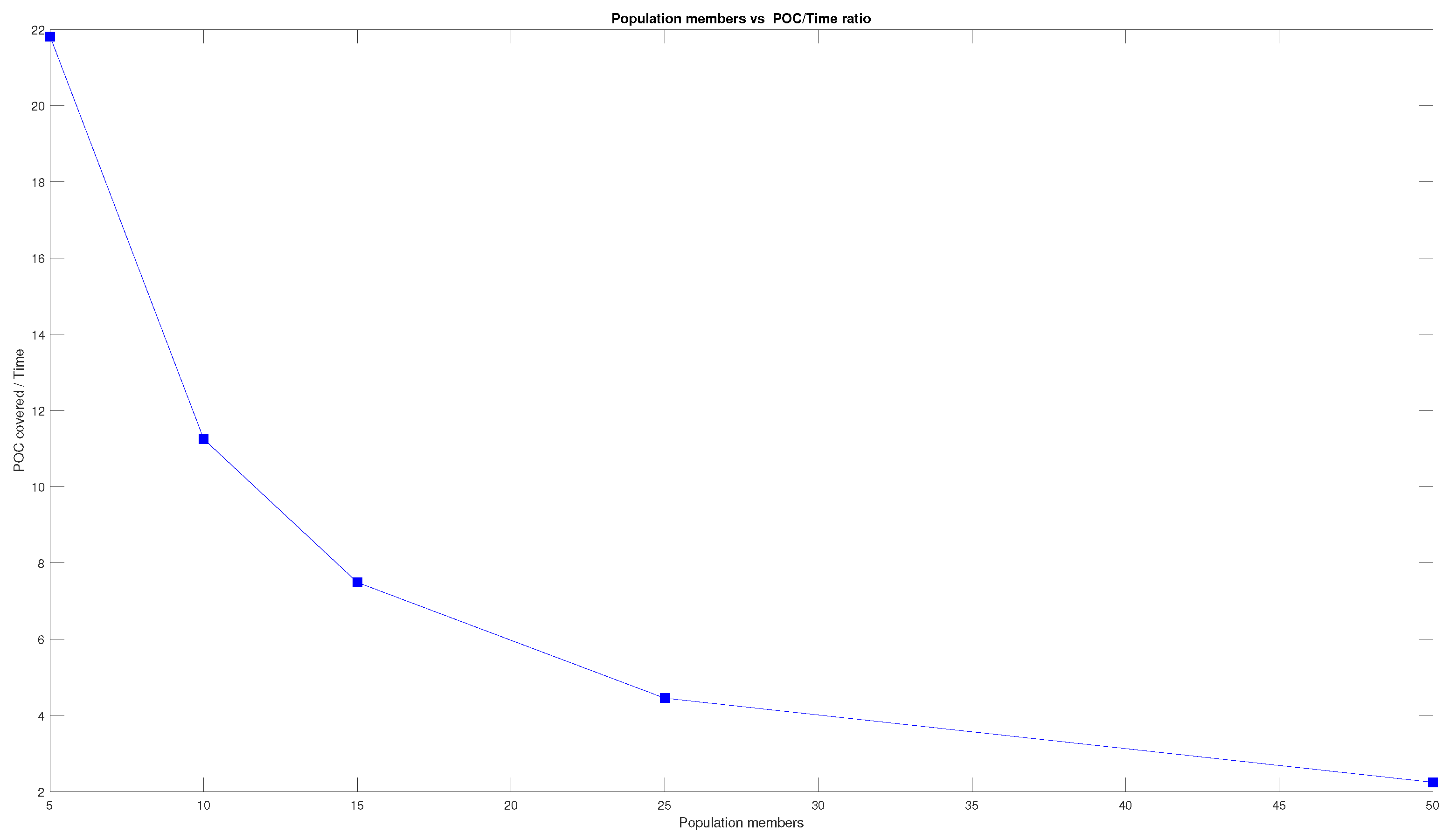
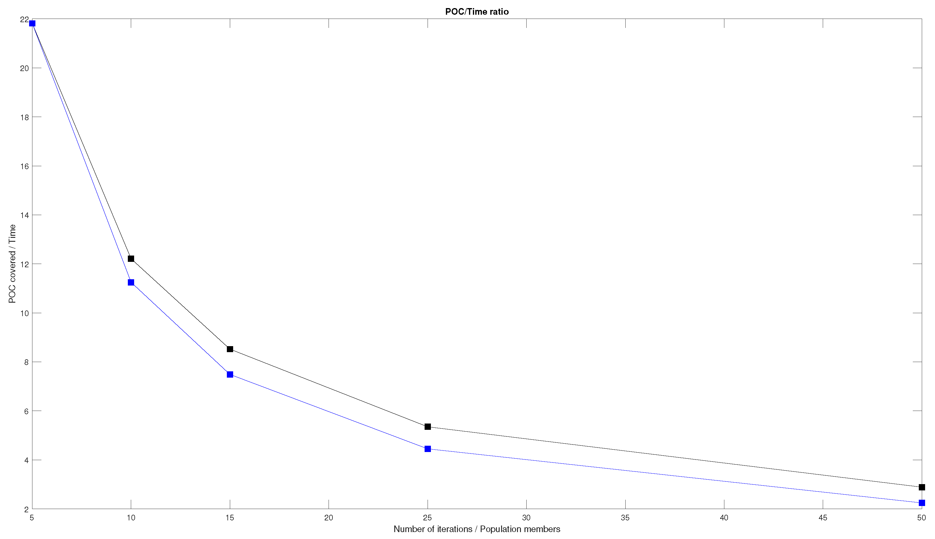
Another interesting piece of data that can be obtained from the tables above is the ratio between the POC covered and the time invested in the calculation of the coverage angle. The evolution of this ratio as the number of members of the population and the number of iterations increase can be seen in
Figure 15 and
Figure 16. As can be seen in the Figures, the ratio is similar for both the increase in the number of iterations and the increase in the number of members of the population.
To better compare the results in both cases, the two graphs are plotted together in
Figure 17. The graph shows that the ratio is in fact similar, even though the one related to the increase in the number of members of the population is slightly greater. This fact does not mean that the POC and execution times are better in this case, as has been debated before in this section, but it means that the relation between the two measures is more distinct.
These graphs show that as the number of members of the population and the number of iterations increase, the ratio between the POC covered and the time invested decreases. This means that we can choose different parameters for the DE algorithm if we want the best possible result not considering the time invested in the calculation of the best angle or a good result obtained in a short amount of time.
Another fact that can be inferred from the data above is that increasing the number of iterations yields a better result than increasing the number of members of the population. As it can be observed in
Table 1 and
Table 2, the final POC covered is greater and the execution time is lower when increasing the number of iterations instead of the number of members of the population.
These results prove the great versatility of the DE algorithm in various situations.
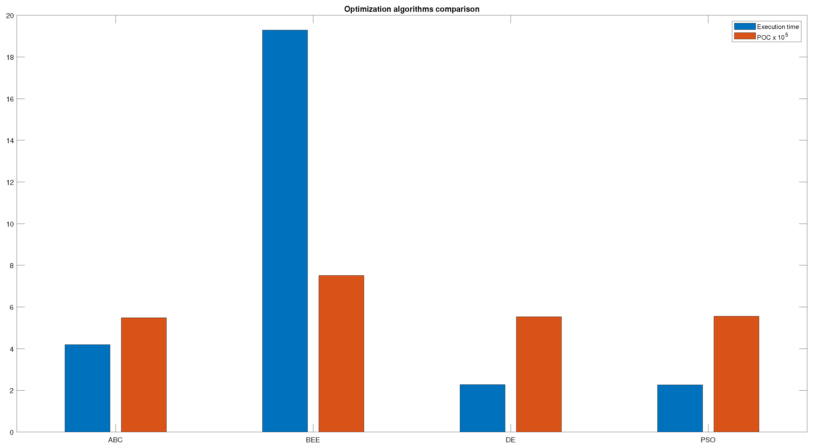
Comparison with Other Optimization Algorithms
As it has been stated in the introduction, this operation could be performed with any optimization algorithm. To further test the results obtained in this work, the path planning algorithm was compared with other known optimization algorithms such as particle swarm optimization (PSO) [
22], the bees algorithm (BEE) [
23], and the artificial bee colony algorithm (ABC) [
24]. The templates for these algorithms are all taken from the work of Yarpiz [
25], including the DE algorithm, to make this comparison fair. Due to that fact, the obtained results for the DE algorithm may differ with the ones shown in the tables above. The parameters for the test are 10 maximum iterations and 25 population members for all algorithms. The comparison can bee seen in
Figure 18:
The red bar indicates the POC and the blue bar represents the execution time needed to complete the optimization. As can be seen in the
Figure 18, all algorithms obtain a similar POC, PSO, and DE being the least time-consuming, while the BEE algorithm obtains the highest POC with the disadvantage of needing as much as 10 times the computation time of the DE and PSO algorithms. Even though the POC obtained by the ABC algorithm is similar to the ones of the PSO and DE algorithms, the execution time is twice as much. These results prove that even though the differential evolution algorithm has been used in this work, any optimization algorithm could achieve similar results. Given that the code for the differential evolution algorithm can be obtained from Yarpiz [
25], a flowchart has been included with the steps of the algorithm (
Figure 8), and the ocean current data have been obtained from the public OSCAR data set [
17], we believe this work is easily reproducible.
To use this algorithm in real missions, the coverage bandwidth and the flight level need to be specified to match the characteristics of the fixed-wing UAV, such as maximum altitude supported and the radius of turn, which is consequently dependent on the airspeed. These parameters need to be properly calculated and specified so that the trajectory calculated by the algorithm is feasible for the UAV.
4. Conclusions
The goal of this study was to design and implement a probabilistic coverage path planning algorithm applied to search tasks in marine environments.
To generate a probability of containment map, a technique involving a marine currents data set and the use of drifters was used. After the drifters were moved by the ocean and wind currents, the probability of containment map was generated by fitting the drifters positions to a Gaussian mixture model.
The differential evolution algorithm was used to test different coverage sweep angles and obtain the best possible solution given a number of members of the population and maximum iterations. Once the best angle was obtained, a feasible coverage path was generated.
The path planning algorithm was tested with a different set of parameters to collect data about the POC covered, the time consumed, and the final coverage angles obtained. From these data, a series of plots was created to better see the evolution of the final result as the members of the population and iterations increased, and to see the evolution of the ratio between time invested in the execution of the algorithm and the results obtained.
All of the steps and the sources for the OSCAR data set and the code used in this work were detailed in this paper; thus, they should be easy to reproduce. Furthermore, the necessary parameters needed to apply the algorithm to any UAV were specified in this paper, so they can be used in real missions.
As a future work, other parameters can be considered for the cost function of the differential evolution algorithm, such as energy consumption of the UAV, and more drones can be added to create a multirobot coverage strategy.


 ,
, 


