
Vision Object-Oriented Augmented Sampling-Based Autonomous Navigation for Micro Aerial Vehicles


Abstract
:1. Introduction
2. Related Work
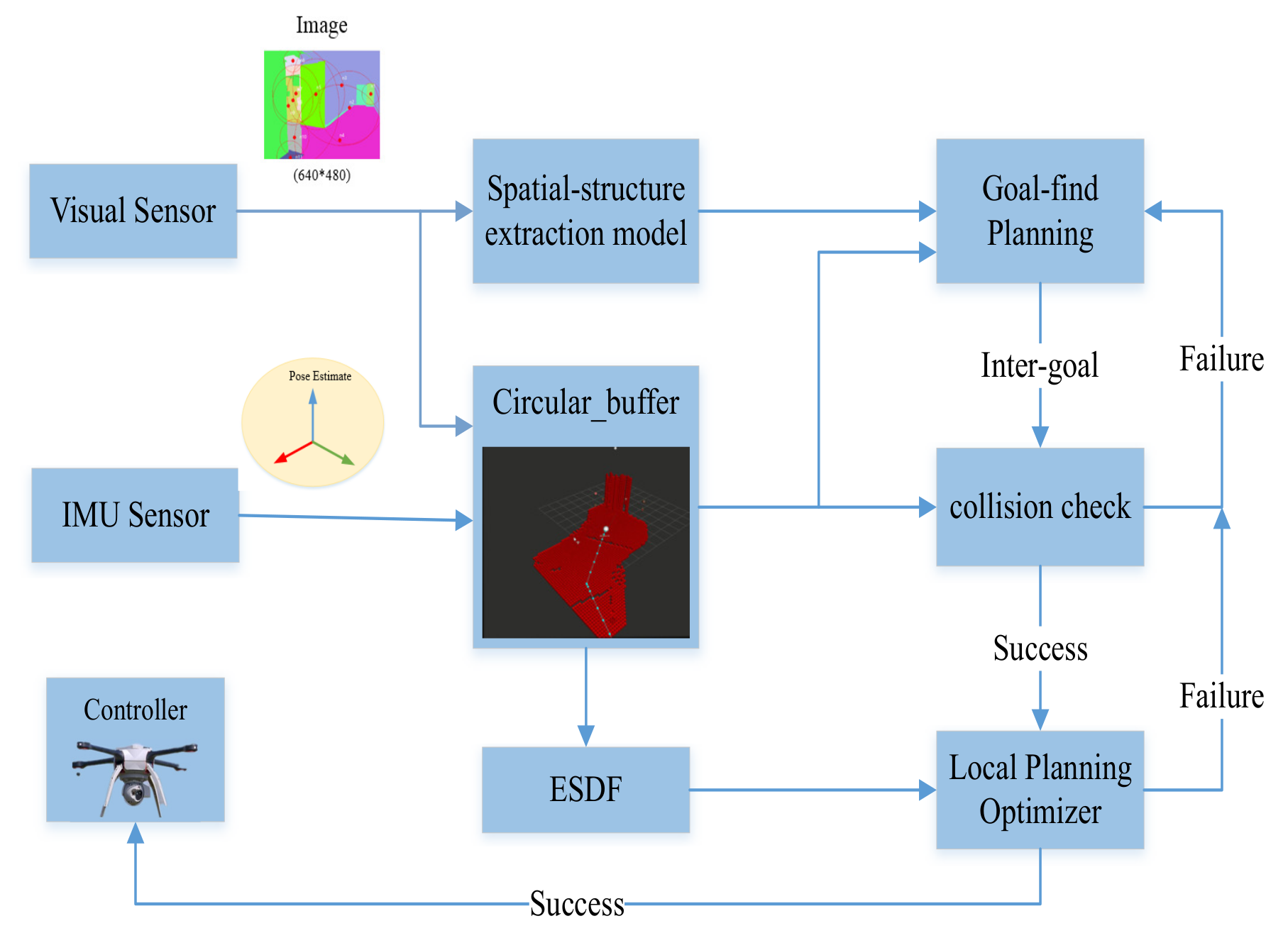
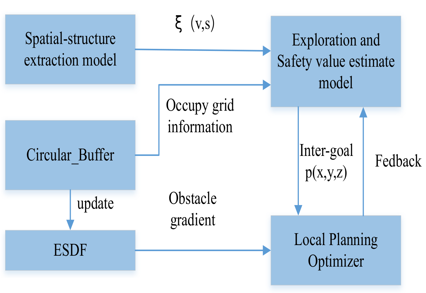
3. System Framework
4. Methods
4.1. Map Representation
4.2. Spatial-Structure Information Extraction
| Algorithm 1 Extracting Spatial-structure Information. |
|
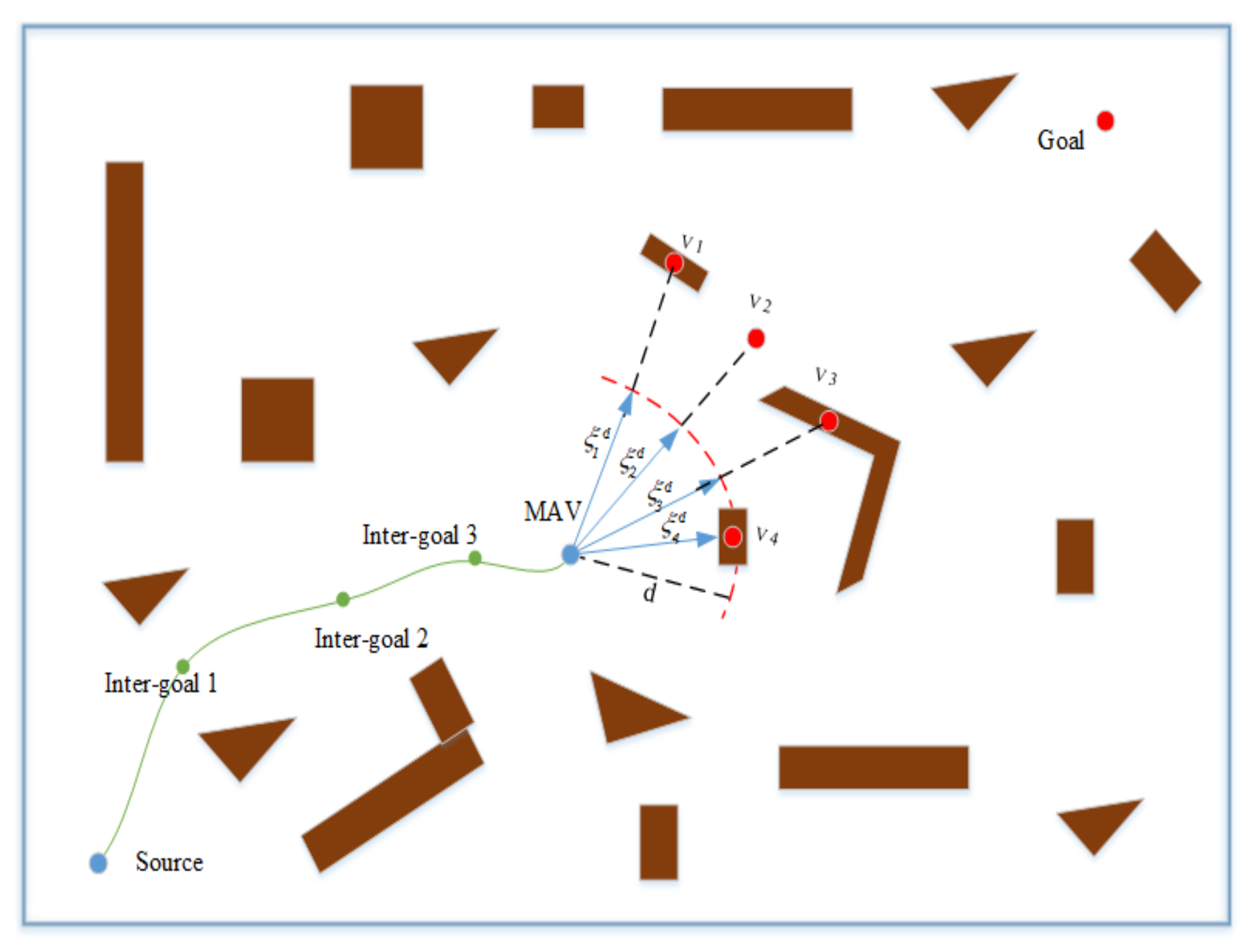
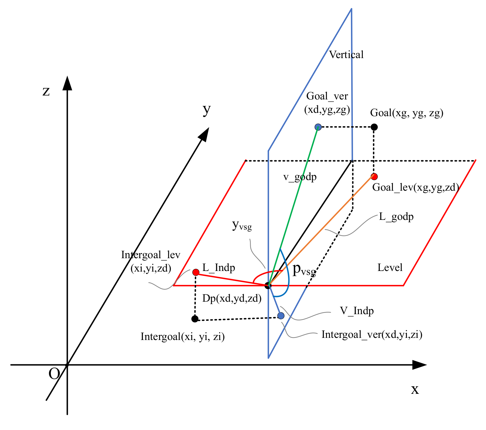
4.3. Intermediate Goal
| Algorithm 2 Obtain Intermediate Goal. |
| Input: Output: for do
|
4.4. Flight Status Switch
| Algorithm 3 Status Swich. |
| Input:
Output: 3: while do switch () 6: case : 9: if then 12: end if if then 15: end if case : 18: if then 21: end if case : 24: if then 27: end if if then 30: end if end switch end while |
4.5. Local Planning Optimization
5. Experimental Results
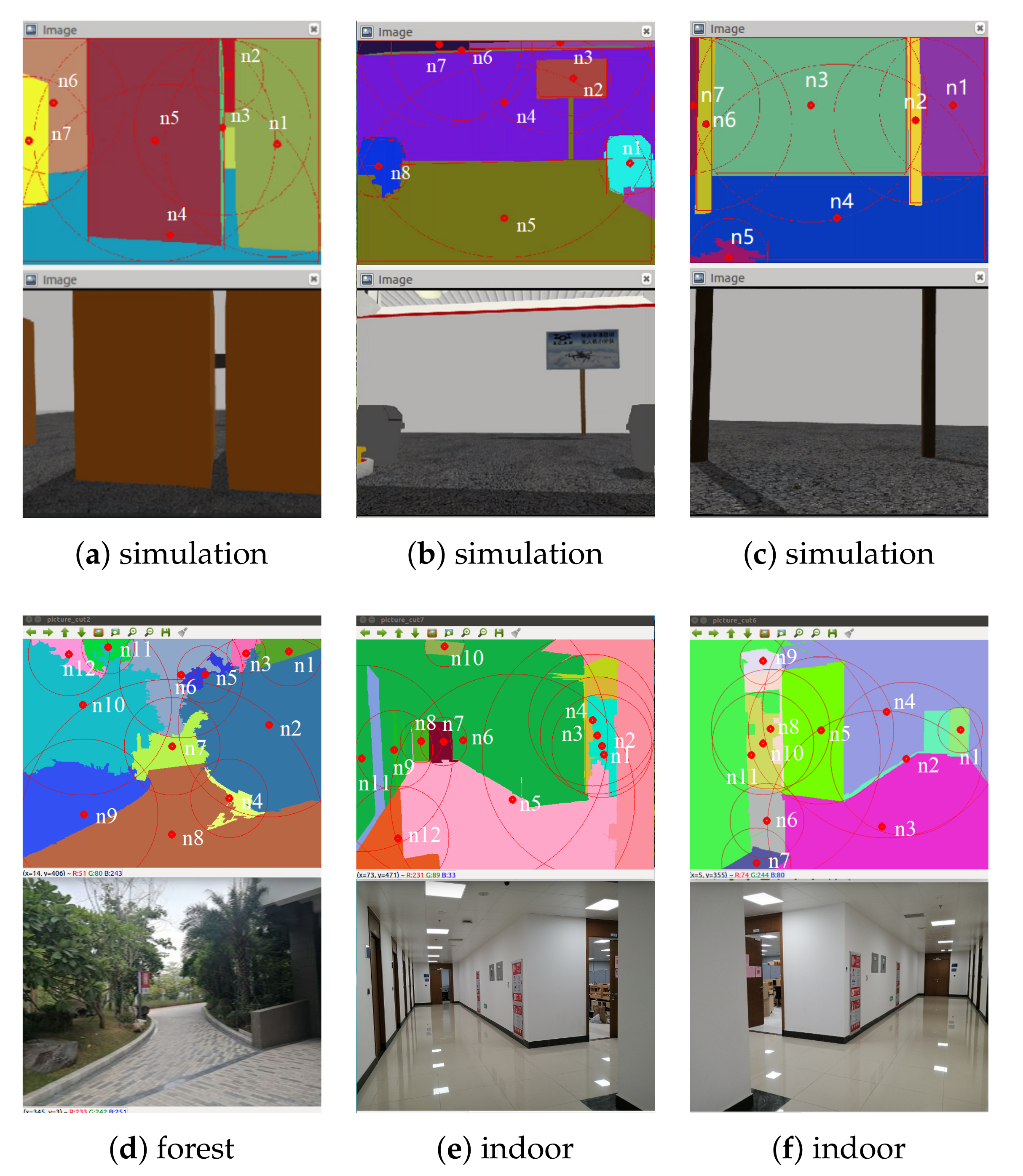
5.1. Spatial-Structure Information Extraction
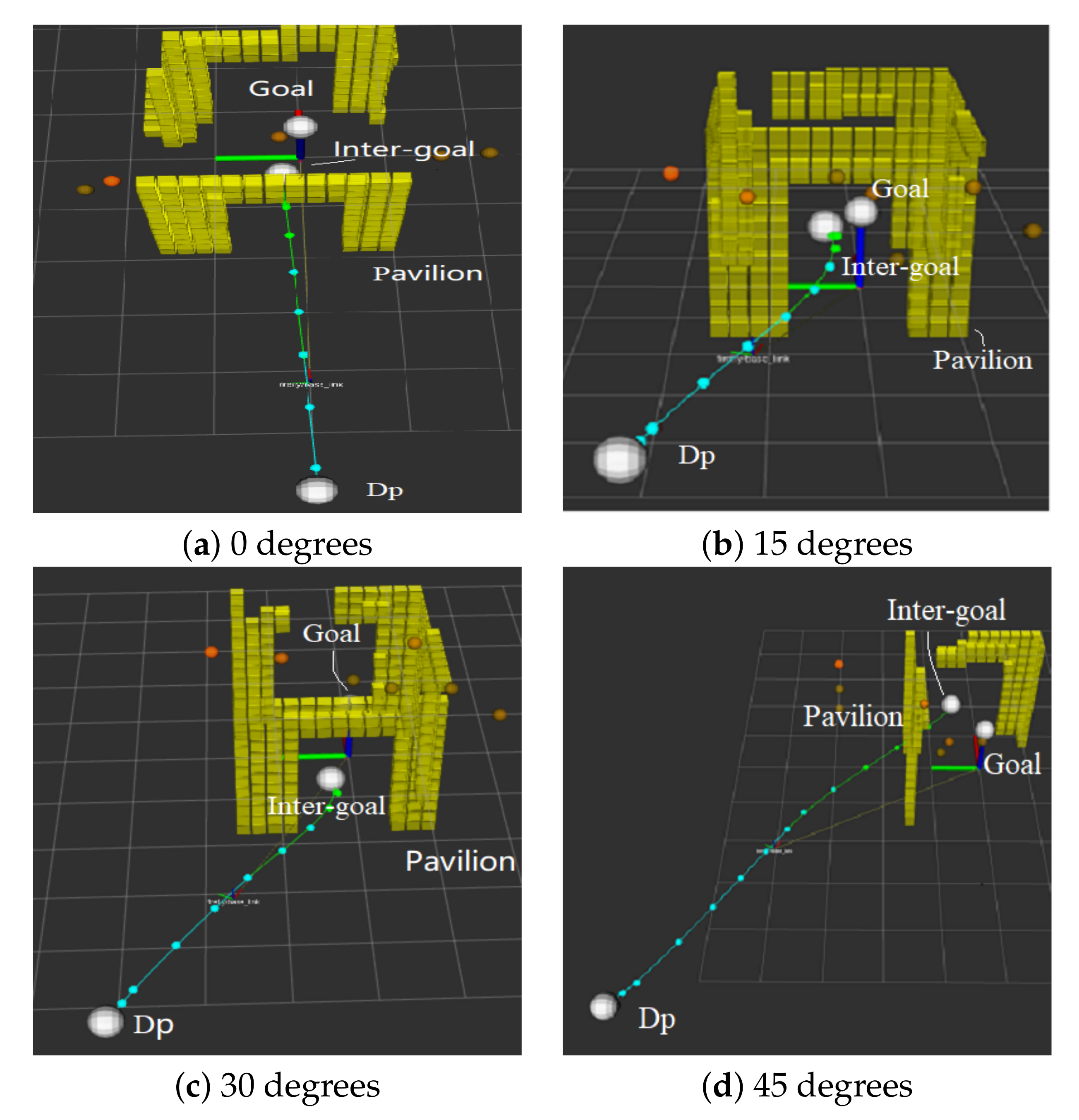
5.2. Across the Gap
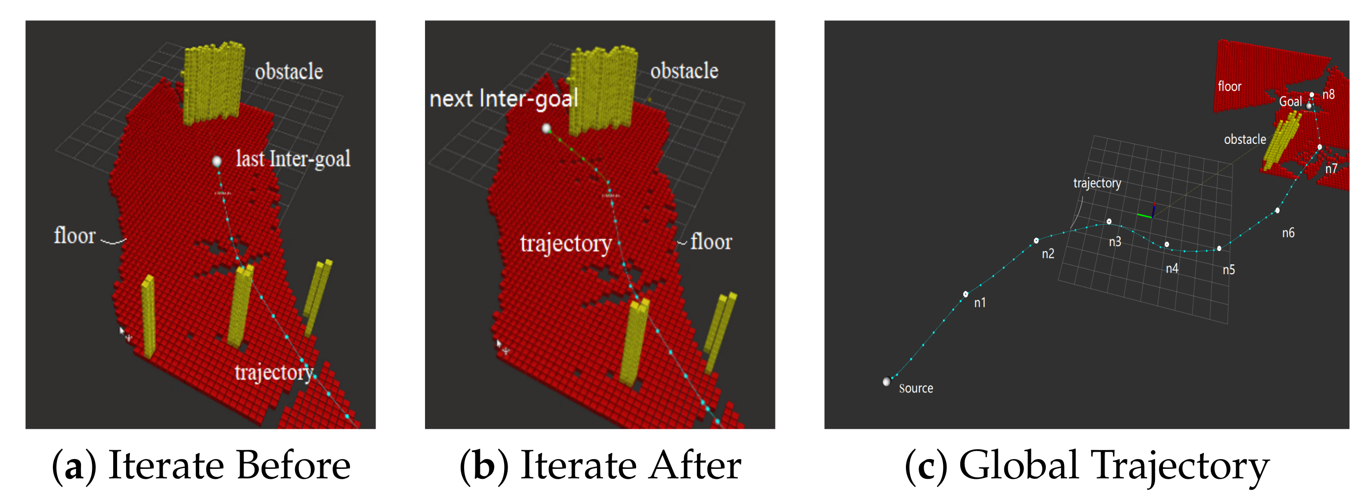
5.3. Local Planning Optimization
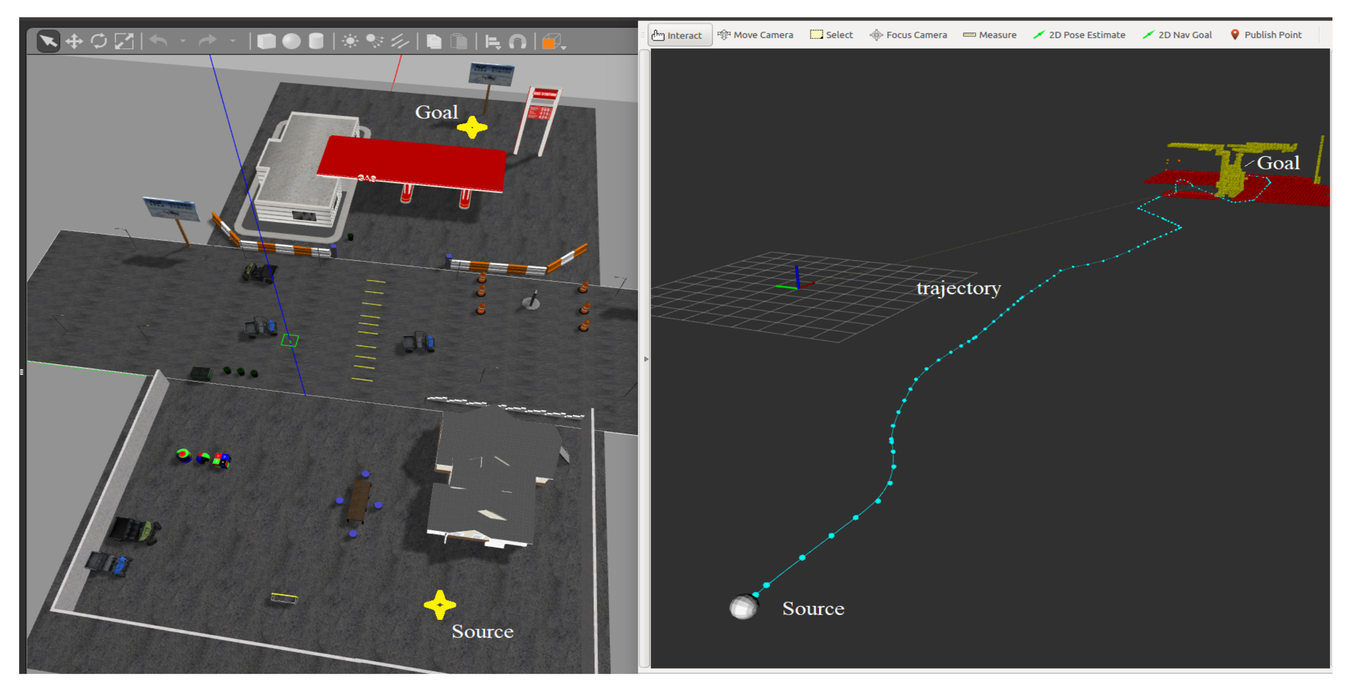
5.4. System Simulation
6. Conclusions
Author Contributions
Funding
Institutional Review Board Statement
Informed Consent Statement
Data Availability Statement
Acknowledgments
Conflicts of Interest
References
- Calisi, D.; Farinelli, A.; Iocchi, L.; Nardi, D. Autonomous exploration for search and rescue robots. In Urban Transport XII: Urban Transport and the Environment in the 21st Century; WIT Press: Southampton, UK, 2007; Volume 94, pp. 305–314. [Google Scholar]
- Thrun, S.; Thayer, S.; Whittaker, W.; Baker, C.; Burgard, W.; Ferguson, D.; Hannel, D.; Montemerlo, M.; Morris, A.; Omohundro, Z.; et al. Autonomous exploration and mapping of abandoned mines. IEEE Robot. Autom. Mag. 2004, 11, 79–91. [Google Scholar] [CrossRef] [Green Version]
- Oleynikova, H.; Taylor, Z.; Siegwart, R.; Nieto, J. Safe Local Exploration for Re-planning in Cluttered Unknown Environments for Microaerial Vehicles. IEEE Robot. Autom. Lett. 2018, 3, 1474–1481. [Google Scholar] [CrossRef] [Green Version]
- Chen, J.; Liu, T.; Shen, S. Online generation of collision-free trajectories for quadrotor flight in unknown cluttered environments. In Proceedings of the 2016 IEEE International Conference on Robotics and Automation (ICRA), Stockholm, Sweden, 16–21 May 2016; pp. 1476–1483. [Google Scholar]
- Alzugaray, I.; Teixeira, L.; Chli, M. Short-term UAV path-planning with monocular-inertial SLAM in the loop. In Proceedings of the 2017 IEEE International Conference on Robotics and Automation (ICRA), Singapore, 29 May–3 June 2017. [Google Scholar]
- Usenko, V.; von Stumberg, L.; Pangercic, A.; Cremers, D. Real-time trajectory re-planning for MAVs using uniform B-splines and 3D circular buffer. In Proceedings of the 2017 IEEE/RSJ International Conference on Intelligent Robots and Systems (IROS), Vancouver, BC, Canada, 24–28 September 2017; pp. 215–222. [Google Scholar]
- Karaman, S.; Frazzoli, E. Incremental Sampling-based Algorithms for Optimal Motion Planning. Int. J. Robot. Res. 2011, 30, 846–894. [Google Scholar] [CrossRef]
- Florence, P.; Carter, J.; Tedrake, R. Integrated Perception and Control at High Speed: Evaluating Collision Avoidance Maneuvers without Maps. In Algorithmic Foundations of Robotics XII; Springer: Cham, Switzerland, 2016. [Google Scholar]
- Lopez, B.T.; How, J.P. Aggressive 3-D collision avoidance for high-speed navigation. In Proceedings of the 2017 IEEE International Conference on Robotics and Automation (ICRA), Singapore, 29 May–3 June 2017; pp. 5759–5765. [Google Scholar]
- Zucker, M.; Ratliff, N.; Dragan, A.D.; Pivtoraiko, M.; Klingensmith, M.; Dellin, C.M.; Bagnell, J.A.; Srinivasa, S.S. CHOMP: Covariant Hamiltonian optimization for motion planning. Int. J. Robot. Res. 2013, 32, 1164–1193. [Google Scholar] [CrossRef] [Green Version]
- Oleynikova, H.; Burri, M.; Taylor, Z.; Nieto, J.; Siegwart, R.; Galceran, E. Continuous-time trajectory optimization for online UAV re-planning. In Proceedings of the 2016 IEEE/RSJ International Conference on Intelligent Robots and Systems (IROS), Daejeon, Korea, 9–14 October 2016; pp. 5332–5339. [Google Scholar]
- LaValle, S.M. Rapidly-Exploring Random Trees: A New Tool for Path Planning; Technical Report; Computer Science Department, Iowa State University: Ames, IA, USA, 1998; pp. 98–111. [Google Scholar]
- Bry, A.; Roy, N. Rapidly-exploring Random Belief Trees for motion planning under uncertainty. In Proceedings of the IEEE International Conference on Robotics and Automation (ICRA), Shanghai, China, 9–13 May 2011. [Google Scholar]
- Bircher, A.; Kamel, M.; Alexis, K.; Oleynikova, H.; Siegwart, R. Receding horizon “next-best-view” planner for 3D exploration. In Proceedings of the 2016 IEEE International Conference on Robotics and Automation (ICRA), Stockholm, Sweden, 16–21 May 2016; pp. 1462–1468. [Google Scholar]
- Dai, A.; Papatheodorou, S.; Funk, N.; Tzoumanikas, D.; Leutenegger, S. Fast Frontier-based Information-driven Autonomous Exploration with an MAV. In Proceedings of the 2020 IEEE International Conference on Robotics and Automation (ICRA), Paris, France, 31 May 2020; pp. 9570–9576. [Google Scholar]
- Witting, C.; Fehr, M.; Behnemann, R.; Oleynikova, H.; Siegwart, R. History-aware autonomous exploration in confined environments using MAVs. In Proceedings of the 2018 IEEE/RSJ International Conference on Intelligent Robots and Systems (IROS), Madrid, Spain, 1–5 October 2018; pp. 1–9. [Google Scholar]
- Amanatides, J.; Woo, A. A fast voxel traversal algorithm for ray tracing. Eurographics 1987, 87, 3–10. [Google Scholar]
- Hornung, A.; Wurm, K.M.; Bennewitz, M.; Stachniss, C.; Burgard, W. OctoMap: An efficient probabilistic 3D mapping framework based on octrees. Auton. Robot. 2013, 34, 189–206. [Google Scholar] [CrossRef] [Green Version]
- Felzenszwalb, P.F.; Huttenlocher, D.P. Efficient Graph-Based Image Segmentation. Int. J. Comput. Vis. 2004, 59, 167–181. [Google Scholar] [CrossRef]
- Burri, M.; Oleynikova, H.; Achtelik, M.W.; Siegwart, R. Real-time visual-inertial mapping, re-localization and planning onboard MAVs in unknown environments. In Proceedings of the 2015 IEEE/RSJ International Conference on Intelligent Robots and Systems (IROS), Hamburg, Germany, 28 September–2 October 2015. [Google Scholar]
- Richter, C.; Bry, A.; Roy, N. Polynomial Trajectory Planning for Aggressive Quadrotor Flight in Dense Indoor Environments. In Robotics Research; Springer: Berlin/Heidelberg, Germany, 2016. [Google Scholar]
- De Boor, C. On calculating with B-splines. J. Approx. Theory 1972, 6, 50–62. [Google Scholar] [CrossRef] [Green Version]
- Cox, M.G. The Numerical Evaluation of B-Splines. IMA J. Appl. Math. 1972, 10, 134–149. [Google Scholar] [CrossRef]
- Furrer, F.; Burri, M.; Achtelik, M.; Siegwart, R. Robot operating system (ROS). In Studies in Computational Intelligence; Springer: Cham, Switzerland, 2016. [Google Scholar]

| Evaluation Metric | Map 1 | Map 2 | Map 3 | Map 4 |
|---|---|---|---|---|
| Path length [m] | 28.284 | 28.284 | 28.284 | 28.284 |
| Ewok time [s] | 25.470 | 25.668 | 28.995 | / |
| Our method time [s] | 32.130 | 36.581 | 39.410 | 36.209 |
| Ewok trajectory length [m] | 28.401 | 32.197 | 33.457 | / |
| Our method trajectory length [m] | 43.830 | 51.220 | 56.469 | 51.343 |
| Ewok success ratio | 100% | 24% | 8% | / |
| Our method success ratio | 100% | 88% | 88% | 92% |
| Evaluation Metric | Map 5 | Map 6 | Map 7 |
|---|---|---|---|
| Path length [m] | 16.0 | 25.0 | 51.0 |
| Our method time [s] | 26.676 | 29.273 | 64.6065 |
| Our method trajectory length [m] | 35.178 | 38.914 | 81.9164 |
| Our method success ratio | 84% | 84% | 64% |
Publisher’s Note: MDPI stays neutral with regard to jurisdictional claims in published maps and institutional affiliations. |
© 2021 by the authors. Licensee MDPI, Basel, Switzerland. This article is an open access article distributed under the terms and conditions of the Creative Commons Attribution (CC BY) license (https://creativecommons.org/licenses/by/4.0/).
Share and Cite
Zhao, X.; Chong, J.; Qi, X.; Yang, Z. Vision Object-Oriented Augmented Sampling-Based Autonomous Navigation for Micro Aerial Vehicles. Drones 2021, 5, 107. https://doi.org/10.3390/drones5040107
Zhao X, Chong J, Qi X, Yang Z. Vision Object-Oriented Augmented Sampling-Based Autonomous Navigation for Micro Aerial Vehicles. Drones. 2021; 5(4):107. https://doi.org/10.3390/drones5040107
Chicago/Turabian StyleZhao, Xishuang, Jingzheng Chong, Xiaohan Qi, and Zhihua Yang. 2021. "Vision Object-Oriented Augmented Sampling-Based Autonomous Navigation for Micro Aerial Vehicles" Drones 5, no. 4: 107. https://doi.org/10.3390/drones5040107
APA StyleZhao, X., Chong, J., Qi, X., & Yang, Z. (2021). Vision Object-Oriented Augmented Sampling-Based Autonomous Navigation for Micro Aerial Vehicles. Drones, 5(4), 107. https://doi.org/10.3390/drones5040107