1. Introduction, Context, and Motivation
In recent years, Unmanned Aerial Vehicles (UAVs) have been proposed for various applications, including inventive delivery methods. In this article, we focus on the specific problem of data delivery with UAVs when radio communication is used and the connectivity is intermittent.
In such networks, UAVs act as data mules in an environment where the communication range is limited, and thus, connectivity is intermittent. UAVs are in charge of collecting data (e.g., messages, videos, images, medical messages, high-resolution photographs [
1]) from a source site and carrying them to a destination site. The use of UAVs is ideally adapted to such scenarios as they provide considerable time savings compared to other types of transport. Nevertheless, these flying vehicles have to operate with limited energy due to their modest size and constrained weight, and they also have limited storage capacity. In addition, for the applications under consideration, data exchanges are subject to time constraints: the UAVs have a time limit for delivering data to destinations. All these constraints have to be taken into account when computing optimized trajectories for UAVs that act as data mules in a collaborative fashion.
The literature is rich with several methods designed to optimize the itineraries of mobile vehicles for predefined delivery missions operating under a set of constraints. Among them, the Pickup and Delivery optimization Problem (PDP) [
2] models the scenario in which a fleet of vehicles must collaboratively achieve a set of transportation tasks. In this model, customers advertise their transportation needs by sending their requests to a headquarter specifying the pickup and/or delivery locations. The aim is then to find a routing solution where vehicles service all requests, satisfying the time windows and vehicle capacity constraints while optimizing a certain objective function such as total distance traveled. Another model is the Pickup and Delivery Problem with a Time Window (PDPTW), which is a generalization of the well-known Vehicle Routing Problem (VRP) [
3] and was originally designed for terrestrial vehicles. The PDPTW optimization problem has inspired much research and has been well studied in the literature in the case of terrestrial vehicles. PDP and PDPTW, as most routing problems, are NP-hard problems [
4]. These classes of problems can only be optimally solved for small instances, and for larger instance, various heuristics are commonly applied. For example, the authors in [
5] proposed a tabu search heuristic to solve the PDP with a time window where vehicles have to transport goods from the origin position to the destination while satisfying load capacity and time constraints. A similar study was proposed in [
6] where the authors considered multiple depots and adopted a genetic algorithm to solve the PDPTW. The work carried out in [
7] also considered multiple depots and proposed three exact solutions to solve the PDPTW optimization problem. A new variant of the PDP called VRP with Simultaneous Delivery and Pickup and Time Windows (VRPSDPTW) was proposed in [
8]. In this variant, the authors introduced five objectives and designed two meta-heuristics, namely Multi-Objective Local Search (MOLS) and the Multi-Objective Memetic Algorithm (MOMA), to solve the proposed optimization problem. Unlike PDPTW for terrestrial vehicles, only a few papers have focused on the PDP optimization problem for flying aerial vehicles. For example, the authors in [
9] focused on data delivery using UAVs. They proposed a SMARTheuristic based on the cluster-first, route-second algorithm to determine UAV routes while minimizing the time needed to satisfy all requests (i.e., pickup data from a source and deliver it to a target). The study in [
10] proposed a pickup and delivery service using both terrestrial and aerial vehicles. The authors developed two algorithms, the vehicle-driven and drone-driven routing heuristics, in order to optimize the planning of the vehicle-drone delivery service. For more details on the extended variants of routing optimization problems for UAV path optimization, the reader can refer to the survey in [
11].
In our study, we focus on the Multi-Objective Evolutionary Algorithm (MOEA) technique to solve the PDPTW using multiple UAVs. We propose to use the elitist Non-dominated Sorting Genetic Algorithm II (NSGA-II) [
12] to find a set of UAV routes minimizing three objective functions described as follows:
Distance traveled: the sum of the distances traveled by all UAVs deployed.
Schedule duration: the total time of all UAVs’ tours. This time starts when a given UAV leaves the depot and ends when it returns. The schedule duration includes the UAV’s flying time to visit the different sites of its tour, the service time at each site, and the refueling time (time to recharge the UAV’s battery), if needed.
The number of vehicles: the total number of UAVs used to perform all tasks.
The solutions sought include not only solutions that minimize one of the objective functions, but also solutions that dominate others over a combination of objectives (e.g., in the sense of Pareto optimality, according to the NSGA-II design). Genetic algorithms, in general, including the NSGA-II, have been applied to several variants of routing problems, such as the Multiple Objective Dial a Ride Problem (MO-DRP) [
13], the bi-objective pickup and delivery problem [
14], or the Pickup and Delivery Problem with Time Windows and Demands (PDPTW-D) [
15].
In [
15], the PDPTW-D optimization problem was proposed for terrestrial vehicles and was formulated as a multi-objective optimization problem. The solutions were then found by an application and adaption of the NSGA-II. To illustrate the efficiency of the proposed NSGA-II algorithm, the authors conducted simulation experiments based on PDPTW test instances created by [
16]. The instances’ definitions and best-known solutions of the PDPTW benchmark problems are available in [
17]. In [
13], the problem was the Dial A Ride Problem (DARP) motivated by the real example of tourist transportation companies in Portugal: a set of drivers are picking up and dropping off customers with minibus vehicles. The multi-objective cost functions that should be minimized are respectively the total distance traveled by the vehicles, the wage difference of the drivers, and the total number of empty seats. The individuals in their NSGA-II variant are vectors that map every customer to a vehicle index. In [
14], the problem was a PDP with just one vehicle (helicopter) and with two objective functions: a total cost that is equivalent to the total distance traveled and the weighted sum of arrival times, where weights give more importance to more urgent requests (unlike our case, which has time windows). The NSGA-II was used as well, and an individual was a single ordered list of sites, corresponding to the pickup site and the delivery site of each task.
The contributions of our study are as follows:
A new formulation of the PDPTW adapted to the UAV context. The new optimization problem is called the PDPTW-UAV.
A new solution of the PDPTW-UAV adapting and applying the NSGA-II algorithm.
Our solution is different from the ones proposed in the literature [
13,
14,
15] because the problem is different. For instance, compared to [
15], our study considers UAVs’ constraints (PDPTW-UAV), whereas their variant was PDPTW-D for vehicles.
A validation of our NSGA-II solution based on the test instances with 100 nodes provided in [
16].
A performance evaluation of our PDPTW-UAV with UAVs’ constraints (such as refueling).
Provide benchmark results for the new PDPTW problem with UAV constraints.
The remainder of our article is organized as follows: In
Section 2, we introduce and precisely define the PDPTW-UAV. In
Section 3, we formalize it as a corresponding mathematical optimization problem. In
Section 4, we describe our adaptation and application of the NSGA-II algorithm, a multi-objective version of a genetic algorithm, to solve the PDPTW-UAV problem. In
Section 5, we first validate the improved NSGA-II, and then, we provide new benchmark PDPTW results for UAVs, useful for researchers in the field. In
Section 6, we discuss some of the sources of uncertainty from the real-world context that can affect our problem solving and how to deal with these issues. Finally, we conclude in
Section 7.
3. PDPTW-UAV: Problem Statement
In our study, we adopted the following notations for the formulation of the proposed PDPTW-UAV. Insights into the mathematical formulation of the variants of the pickup and delivery problems can be found for instance in [
4]. The general case is that each site can be a pickup or delivery site for an arbitrary number of tasks. Our formulation assumes that a site is either the pickup site or the delivery site of exactly one task: this does not lose any of its generality since as many virtual sites can be created at the same location as there are tasks to be picked up or delivered at a site.
N: the set of vertices or sites (any site is either a pickup or a delivery location); it is partitioned as defined below.
n: the number of pickup sites.
p: the number of delivery sites; we consider only the case of paired pickups and deliveries; hence, .
P: the set of pickup vertices .
D: the set of delivery vertices .
0: the depot or central entity location.
K: the set of UAVs.
: the demand/supply at vertex i; .
: the service duration at vertex i; .
: the cost in terms of the duration of the travel of UAV k from vertex i to vertex j.
: the energy consumed by the UAV from vertex i to vertex j.
: the time window for pickup or delivery at vertex i.
: the waiting time at vertex i if a UAV reaches i before .
E: the energy capacity of each UAV.
C: the storage capacity of each UAV.
R: the refueling duration necessary for refueling or changing the battery.
Without loss of generality and for the ease of mathematical formulation, we also assume a numbering such that the pickup task at vertex is paired with a delivery task at vertex with exactly .
3.1. Binary Variables
In our PDPTW-UAV, we define two binary variables:
: one if the kth UAV goes straight from vertex i to vertex j.
: one if the kth UAV refuels its battery at vertex i.
3.2. Fractional Variables
Let and E be three fractional variables used in our problem model for UAV load, UAV service time, and UAV energy, respectively.
: the load of UAV k when leaving vertex i
: the time of the beginning of the service of UAV k at vertex i
: the remaining energy of UAV k after visiting vertex i.
: the additional refueling time of UAV k before leaving vertex i.
3.3. Problem Model
The PDPTW-UAV model can be written by minimizing the following objective functions:
subject to:
The objective function (
1) minimizes the total flight time of UAVs to satisfy all tasks: we assume a constant speed, which is equivalent to minimizing the total flight distance. The objective function (
2) minimizes the total schedule duration, which is the sum of the flight time, waiting time, service time, and refueling duration if needed for all the UAV routes. The last objective function (
3) minimizes the number of UAVs used.
The model constraint (4) ensures that each task is served exactly once. The constraints (5)–(7) guarantee that every UAV leaves the depot and returns to it only once during its tour and that the same UAV that enters a node leaves the node. The constraint (8) is to check the additional schedule time due to the refueling operation. The constraint (9) is the precedence constraint to check that the pickup task is satisfied before its corresponding delivery task, and the constraint (10) ensures that both tasks are serviced by the same UAV. The constraints (11) are the schedule time constraints. Constraints (12) are the time window constraints in which a service time cannot be started after the latest time, and if a UAV arrives before the earliest time, it has to wait until the earliest time to start the service. Constraints (13) and (14) aim at satisfying the storage capacity of each UAV. Finally, the constraints (15) and (16) consist of first checking the remaining UAV energy, then indicating whether refueling is necessary.
4. Solving the PDPTW-UAV Using the NSGA-II
Version 2 of the Non-dominated Sorting Genetic Algorithm [
12] (NSGA-II) is designed to solve multi-objective optimization problems. In our study, we applied the NSGA-II, as illustrated in Algorithm 1, to solve our PDPTW-UAV. The proposed use of the NSGA-II algorithm starts by generating an initial
P population of
N individuals. Then, at each iteration, the NSGA-II randomly selects two individuals called parents from the
P population, applies a crossover operator (
Section 4.1.2) to them to obtain two new individuals called children, which will be mutated (
Section 4.1.3) before being added in the new offspring
Q population. Both parents and offspring populations are merged into a single set called
R. Based on the non-dominated sorting approach and crowding distance sorting [
12], only the best solutions passing the selection step are kept and included in the population of the next iteration
, while the other individuals are removed. Let
, where
is the set of solutions in the Pareto front of level
i.
If only a few solutions of the last front
should be kept in
, these solutions are chosen to have the best crowding distance. Therefore,
solutions will be chosen from the last front set
, where
N is the size of the population and
T is the sum of the size of sets
.
Figure 2 illustrates the non-dominated sorting genetic algorithm process.
The principles of the NSGA-II are based on non-dominating sorting techniques, crowding distance techniques, and elitist techniques. The NSGA-II is characterized by the fact that it first provides solutions close to the Pareto-optimal ones, then it allows for a diversity of solutions, and finally, it preserves the best solution at each iteration for the next iteration.
Although the NSGA-II is an excellent algorithm for solving multi-objective optimization problems, it may require a large number of iterations and a long runtime to converge to the best solutions found. To speed up the convergence of the NSGA-II, we propose to generate good individuals for the initial population, as illustrated in Algorithm 2, and also to improve each individual of the offspring population.
| Algorithm 1 NSGA-II for PDPTW-UAV. |
- 1:
N: {Population size} - 2:
: {Initial population} - 3:
P: {Parent population} - 4:
Q: {Offspring population} - 5:
fordo - 6:
∪ Generate Individual {After improvement} - 7:
end for - 8:
- 9:
whiledo - 10:
for do - 11:
randomly selected from - 12:
Crossover - 13:
Mutate - 14:
Improve {As explained in Section 4.2} - 15:
Compute fitness values of - 16:
Add to - 17:
end for - 18:
{Combing parent and offspring population} - 19:
result of a fast non-dominated sort of - 20:
- 21:
- 22:
while do - 23:
- 24:
- 25:
end while - 26:
{i now corresponds to the first set , which cannot be entirely included in } - 27:
Compute the crowding distance in - 28:
- 29:
- 30:
end while
|
| Algorithm 2 Generate individual. |
- 1:
{list of all tasks} - 2:
{list of tasks served by } - 3:
{task} - 4:
{pickup task} - 5:
{delivery task} - 6:
; {indicates the number of UAVs} - 7:
whileL is not empty do - 8:
- 9:
Select paired tasks randomly from L - 10:
Append to - 11:
Remove from L - 12:
repeat - 13:
the list of paired tasks of L that could be added to without violating constraints (including refueling) - 14:
if T is not empty then - 15:
Select the in T that minimizes the total flying distance increase, when added to - 16:
Append to - 17:
Remove from L - 18:
end if - 19:
until T is empty - 20:
- 21:
Evaluate fitness functions - 22:
end while
|
4.1. Genetic Operations
In this section, we specify the terminologies used for the NSGA-II [
12] and the main elements of the genetic algorithm (individual or chromosome, crossover, and mutation).
4.1.1. Individual Representation
In genetic algorithms, a population is defined as a set of individuals called chromosomes, where each of them could be seen as a solution to the problem to be solved. Each individual is made up of a set of variables known as genes that form the chromosome. In our optimization problem, an individual is a vector of UAV IDs. The size of this vector is equal to the number of tasks to be performed. Each position in the vector refers to a task ID. Then, each UAV is a gene, and it occupies a cell of the vector. In our individual representation, a UAV should appear in at least two cells, reflecting the fact that the pickup task and the corresponding delivery task are served by the same UAV.
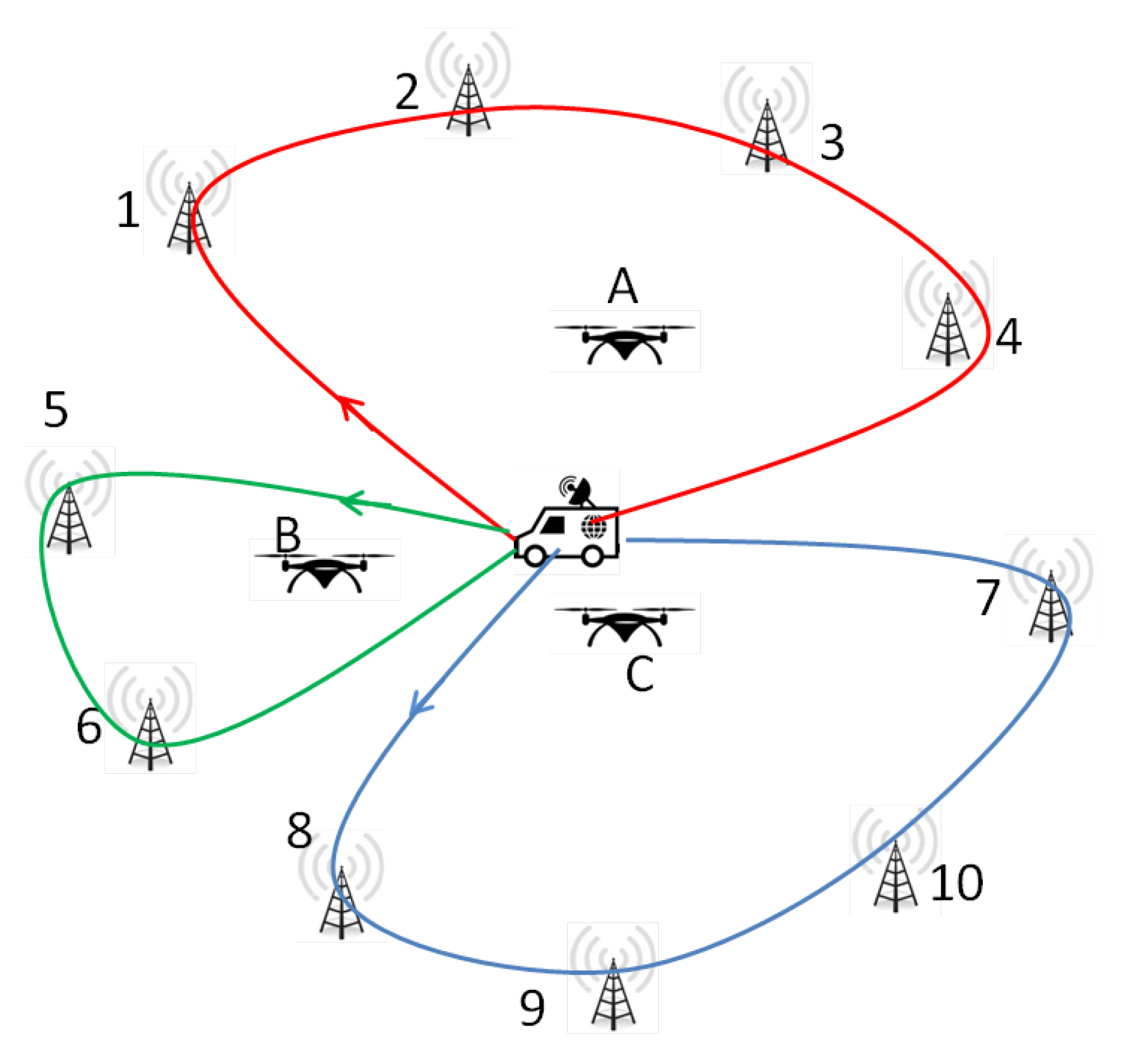
Consider the example of a pickup and delivery problem with 10 tasks specified in
Table 1: each of the tasks, identified by a task ID, is paired with another corresponding task with a different task ID and with the opposite action. The numbering in the problem definition can be arbitrary (contrary to the mathematical formulation), and in the implementation, the “Action” column can be deduced from the action of the associated task.
Figure 3 illustrates an example of an “individual” solution to satisfy the problem.
In this solution, three UAVs are used, denoted:
A,
B, and
C. The UAV
A is associated with tasks with the identifiers 1, 2, 3, and 4; the UAV
B with Tasks 5 and 6; and the UAV
C with Tasks 7, 8, 9, and 10. A possible corresponding tour of the UAV could be represented as in
Figure 1. Although the tour of each UAV starts and ends at the depot, the depot is not considered as a task to be served and does not appear in the individual representation. The order of the tour itself is determined as described in
Section 4.2.1.
We define a valid individual as a solution for which the assignment of tasks to UAVs (represented by the gene vector) satisfies the constraints defined above. In our problem, we generate each initial individual as described in Algorithm 2 to get an initial population of valid individuals and to speed up the convergence of the NSGA II. The random aspect of the generation of individuals comes from the random selection of the first task assigned to a UAV tour.
Then, a greedy selection of the other tasks assigned to the UAV is made as follows. The algorithm iteratively selects the “best” task, i.e., the one that minimizes the distance traveled by the UAV while satisfying the previously mentioned constraints (refueling constraints, capacity constraints, visit time constraints, and maximum travel time constraints). This process is carried out until it is no longer possible to add new tasks to the current UAV tour, in which case, the next UAV tour is generated (if necessary). Thanks to this greedy initialization, the initial individuals not only satisfy the constraints, and are therefore valid individuals, but they already perform well in terms of the objective functions (
1) and (
3).
4.1.2. Crossover Operation
The crossover operation is the action of generating an offspring population from a valid population. It consists of exchanging genes between two parents and creating new children inheriting characteristics of both parents. In our problem, the offspring population is obtained based on the two-point crossover operation [
18]. In this operation, two individuals are selected, and the vector corresponding to each of them is fragmented into three parts on the basis of two randomly chosen vector positions. The first child vector is a recombination of two fragments from Parent 2 and one fragment from Parent 1, and the second child vector is created from the remaining fragments of both parents, as illustrated in
Figure 4.
To obtain an offspring population composed of valid individuals, we make some modifications to the genes of the children to satisfy the constraints of our problem.
4.1.3. Mutation Operation
In genetic algorithms, a mutation is a random alteration of certain genes. In our optimization problem, a mutation operation consists of, on the one hand, randomly selecting a site belonging to the tour of one UAV and, on the other hand, injecting this site into the tour of another UAV. This operation is repeated
k times.
k is randomly selected. The individual resulting from the mutation operation may need a few corrections to become a valid individual, as in the case of the crossover operation. The mutation operation is illustrated in
Figure 5.
4.1.4. Selection Operation
The solutions are first sorted using a non-dominated sorting method in ascending order , and in each Pareto rank, the points are sorted according to crowding distance in descending order. If only a few solutions of the last front need to be added to , these solutions are chosen to have the best crowding distance.
To select the best solutions from the
set that can ensure the preservation diversity, a measure of solution density in the objective space is used. As defined in [
12], we used the crowding distance to estimate the density of solutions surrounding a particular solution in a non-dominated
set. As shown in
Figure 6, the crowding distance of the
solution corresponds to the semi-perimeter of the cuboid whose vertices are the closest neighbors of the solution
i.
4.2. Heuristic Algorithms
In this section, we describe the different heuristics used in the NSGA II algorithm to improve the PDPTW solutions and to speed up its convergence.
4.2.1. Refinement UAV Task List Algorithm
The order in which a UAV visits the set of tasks to be served is very important. It decides the order of the UAV’s tour, its length, its duration, and the number of times the UAV needs to refuel. In our study, we propose a branch and bound algorithm to refine each UAV task list according to the following constraints:
The visiting time for each task must be satisfied. Thus, the UAV must start the task service between its earliest and latest times.
The pickup task must be served before the corresponding delivery task. Note that a UAV can serve several tasks between a pickup and its corresponding delivery task if the UAV’s capacity constraint is fulfilled.
UAV capacity constraints must be met.
The refueling requirement rules must be applied.
The objective is to minimize the travel distance (or equivalently, the duration of the flight). The travel distances of the best candidate solutions, already visited and valid, can be used as the upper bounds in the branch-and-bound search. This allows quickly discarding some branches that would correspond to necessarily worse candidate solutions. This refinement algorithm provides a near-optimal, but not absolutely optimal solution since we do not enumerate all refueling possibilities. In the solutions considered, a UAV only refuels when its remaining energy is not sufficient to reach the next site.
4.2.2. Individual Improvement Algorithm
A valid individual could be improved by reducing the total flight distance of UAVs and the number of UAVs deployed. For this, we first propose a greedy algorithm that, iteratively for each task, tries to place it in the best UAV task list, so that the total flight distance is reduced. Then, we propose an additional greedy algorithm that reduces the number of UAVs used to serve all tasks.
In this algorithm, we reduced the number of UAVs by eliminating the smallest tours if possible. To do this, we sorted the UAV’ tours according to their number of tasks. Then, we tried to insert all the tasks from the smallest UAV tour into the other UAV tour as long as no other changes were made to the individual.
4.2.3. Individual Correction Algorithm
Crossover or mutation operations are very important in genetic algorithms. While the crossover operation enables generating new offspring and finding new solutions that converge to a local minimum, the mutation is a divergence operation that tends to add new genetic characteristics in order to perform a global search on the space of solutions and to avoid the local minimum. After the application of the crossover or mutation operations, the resulting individual may not be valid, as described in
Section 4.1.2 and
Section 4.1.3.
In order to obtain a valid individual after applying the crossover or mutation operations, we proceed as follow:
4.3. Refueling Constraints’ Verification Algorithm
In the previously defined algorithms, the constraints must be checked to ensure the validity of the individuals. Each of them is associated with sub-algorithms. For the specific case of refueling constraints, an algorithm is defined in this section. In order to avoid obtaining an invalid individual, the algorithm checks the refueling constraints each time the individual is modified (generation, mutation, crossover, individual improvement).
Note that energy limitation is one of the major constraints for UAVs. In our study, we assumed that each UAV can refuel during its tour at any site it visits. The refueling process can have an impact on the schedule times. Indeed, the UAV must travel to the site to serve during a time window delimited by the earliest and latest time of the given problem instance. As a result of the refueling process, the UAV may be delayed and be forced to reach a site after the last authorized time. For this purpose, we designed the refueling constraints’ verification algorithm that actually tries to compute the schedule while considering refueling time.
This algorithm is called for each task list of the individual’s UAV. It determines if the individual is valid or not, and if so, it obtains the total schedule time. Algorithm 3 illustrates the steps of calculating the schedule times with refueling.
Algorithm 3 considers two cases to calculate the refueling time: the first one is when a UAV arrives at a site before its earliest time, and the second case is when it arrives after its earliest time and before its latest time. After some initialization (Lines 1–12), the algorithm starts by checking whether the UAV reaches a site before or after its earliest time (Line 13). If the UAV reaches a site before its earliest time, then the algorithm computes a waiting time (Line 14) that could be considered when performing the UAV’s refueling (Line 15). In Lines 15 to 27, the algorithm checks whether the UAV’s refueling is needed or not. If this is the case, then the refueling operation will start at the waiting time, and it can last until the service time (Line 19) or even exceed it (Line 25). Line 28 of the algorithm is executed when the UAV reaches a site after its earliest time and before its latest time. The refueling is performed if the UAV does not have enough energy to serve the current site and reaches the next site (Lines 32–34). Additional time is added to the scheduled time, if the refueling time exceeds the service time (Lines 38–39).
| Algorithm 3 Refueling algorithm for a UAV tour/. |
- 1:
UAV maximum autonomy; {E is the remaining UAV energy expressed in flight duration} - 2:
0; {Waiting time} - 3:
UAV task list - 4:
- 5:
: {time to travel from the previous task site to the site of the i-th task of the task list l} - 6:
: {earliest time} - 7:
: {latest time} - 8:
: {service time} - 9:
: {Full refueling time (constant)} - 10:
fordo - 11:
- 12:
- 13:
if then - 14:
- 15:
if then - 16:
- 17:
- 18:
else - 19:
{need refueling during the service time and the waiting time} - 20:
- 21:
if then - 22:
- 23:
- 24:
else - 25:
- 26:
end if - 27:
end if - 28:
else if then - 29:
if then - 30:
- 31:
- 32:
else - 33:
{need refueling during the service time} - 34:
- 35:
if then - 36:
- 37:
- 38:
else - 39:
- 40:
end if - 41:
end if - 42:
else - 43:
{Refueling not possible; the individual is not valid} - 44:
end if - 45:
end for
|
6. Coping with Uncertainties and a Real-World Scenario
In this article, we considered the PDPTW-UAV, which can be mathematically and exactly formulated as in
Section 3, Equations (
1)–(16). We proposed the NSGA-II algorithm to solve it. However, when considering the problem in the real world, the formulation is no longer accurate.The goal of this section is to give an overview and relevant references to solve the problem when uncertainties exist. Indeed, each constraint, such as the battery capacity, is known up to a certain approximation and, in addition, can be subject to random events, for instance the travel time from Point A to Point B; think of a situation with strong wind. In a case where the constraints are not really strict constraints, it is possible to solve the problem with the expected values, to consider the most pessimistic scenarios, or to include margins of error, for example to add
to the travel time to account for the uncertainties.
However, more methodologically sound approaches have been adopted: many researchers have properly formalized new variants of the considered problems that explicitly take into account randomness and uncertainty. One example of such variants is the “stochastic vehicle routing problem(s)” extending the “vehicle routing problem” with several options, and some related surveys can be found in [
19] or [
20], for instance.
Following [
19], there exist two main approaches to cope with uncertainties. The first one is to write a Chance-Constrained Program (CCP) where the constraints can be satisfied with identified probabilities due to stochasticity; a solution still has to optimize an objective function, but now, the probability that it fails is bounded by an additional parameter. The second is to actually take into account the probability of failing to satisfy a constraint during the plan execution, then being able to react through recourse: these are Stochastic Programs with Recourse (SPRs). In the last case, the recourse might be pre-planned and its cost integrated in the objective function, or alternately, the solution might be updated dynamically during plan execution, or the problem might be solved online [
20]. In all cases, effort is required, as the problem becomes more complex: for instance, for the CCP, the simple calculation of the objective function of a given candidate solution may require the resolution of another optimization problem. Numerous approaches have been proposed; recently, machine learning has been used for solving the class of VRP problems (see [
21]); for intractable settings, it is an example of how stochastic constraints or demands may be incorporated ( see Appendix [C.6] in [
21].
In the following, we list some examples of sources of uncertainties that may affect the problem solving of our UAV planning mission:
general reliability of the drone with respect to the mission (mean time to failure),
external incident (like physical attacks on drones, eagle hunting, etc.),
travel time that can be subject to weather conditions,
consumed energy that can be subject to weather conditions or rotor engine conditions,
energy capacity, which can be affected by battery aging,
service duration, which depends on the actual throughput to transfer data
positioning precision, which depends on the precision of the embedded localization system
The uncertainties may have an impact both on the variables and on the methodology that would be used. For real deployments of the PDPTW-UAV, in general, arguably one of the most important issues is the ability to recover the UAVs; hence, we would suggest formulating an extended version problem with the family of stochastic programs with recourse so that it includes a plan to recover the drone. Our proposal would constitute a baseline and benchmark for such extended approaches.
Real-world context:
Another problem from a real-world scenario that is worth discussing is that of gathering information about the requests of nodes in a network that does not provide full connectivity, in order to compute UAV tours by our algorithm in a centralized manner.
A real-world example could be that of nodes that are capturing images, videos, or time series from sensors with a high sample rate, therefore accumulating large volumes of data. One would make requests for the UAV transport of the data. The requests are considered as small packets and could be collected through a Low-Power Wide-Area Network (LPWAN) with very wide coverage, such as Long Range (LoRa) technology. The LPWAN network would be insufficient to transmit all the raw data (range of several kilometers for a LoRaWAN gateway, but with only a few bytes/seconds available per node with LoRa in practice). Instead, based on the requests, the proposed NSGA-II algorithm will compute the drones’ tour where the large volumes of data can be carried out by these flying vehicles. Another option is to collect requests during the UAVs’ tour while they are serving sites. The collected requests will be used by the NSGA-II to calculate the next tours. Machine learning could also be used to predict and optimize the computation of the upcoming UAVs’ tour.
7. Conclusions
In this paper, we applied the NSGA-II to solve the pickup and delivery optimization problem with a time window with an intermittent connectivity network using UAVs, called PDPTW-UAV.
One of the main differences from previous studies is that we were able to introduce UAV constraints (such as refueling) in our variant of the NSGA-II. We were able to add a refueling constraint verification algorithm to our variant of the NSGA-II, because it is modular. The refueling constraint verification can be modified arbitrarily, to compute the most realistic energy consumption model, etc., without modifying other parts of the algorithm.
For this purpose, we introduced a new representation of individuals (genes), as well as a number of associated heuristics and algorithms for generation, crossover, and mutation. Several experiments were conducted with and without the consideration of a refueling constraint. The results presented in this paper clearly show that NSAG-II is capable of achieving excellent results when applied to the PDPTW-UAV problem.
In our future work, we plan to optimize the management of the refueling operations, and we will also propose a formula to make the refueling time proportional to the amount of energy required by the UAV.


