Deep Learning Classification of 2D Orthomosaic Images and 3D Point Clouds for Post-Event Structural Damage Assessment


Abstract
1. Introduction
2. Literature Review
2.1. Studies Used 2D Images for Detection and Classification
2.2. Studies Used 3D Point Clouds for Detection and Classification
2.3. Knowledge Gap
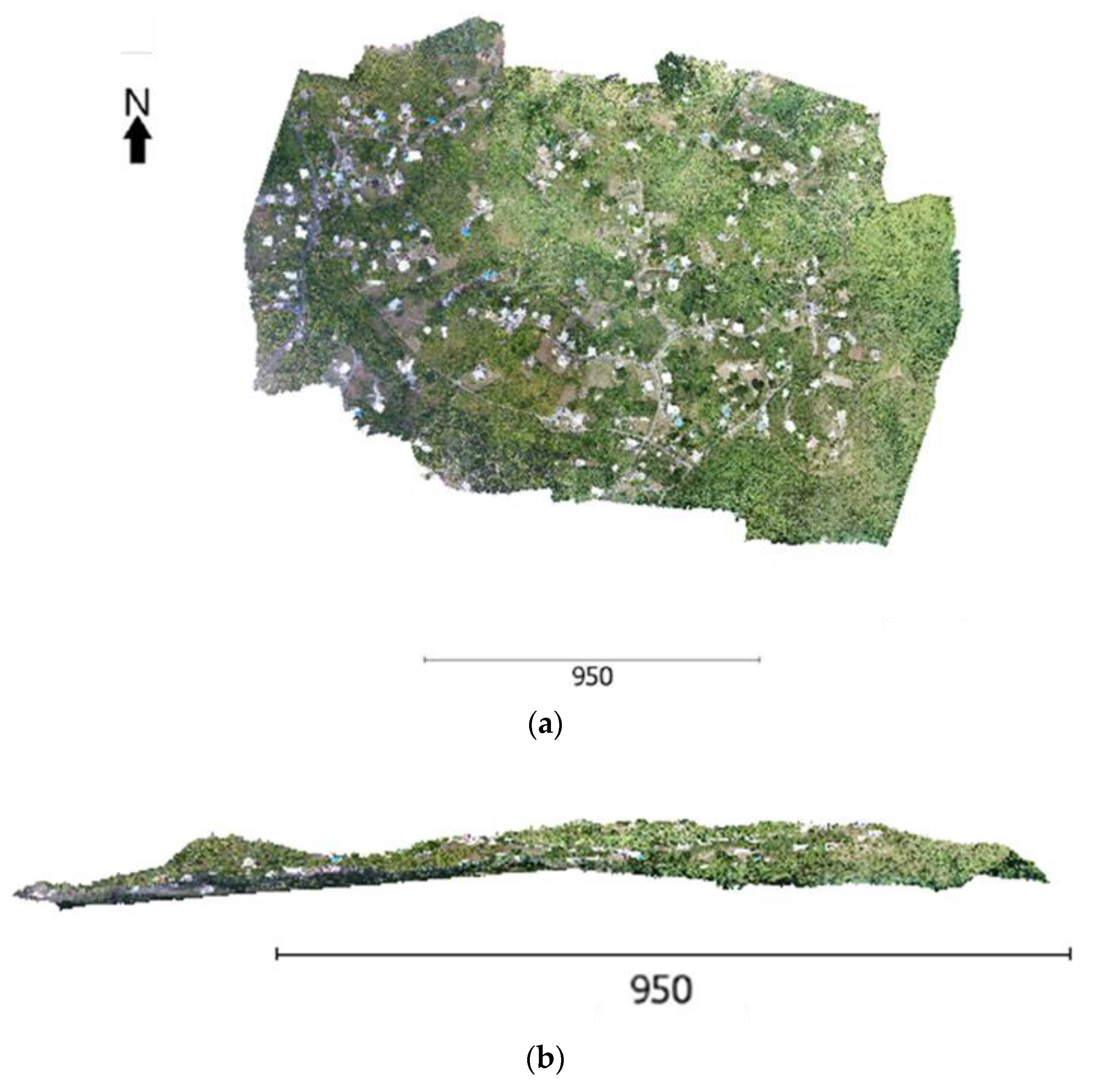
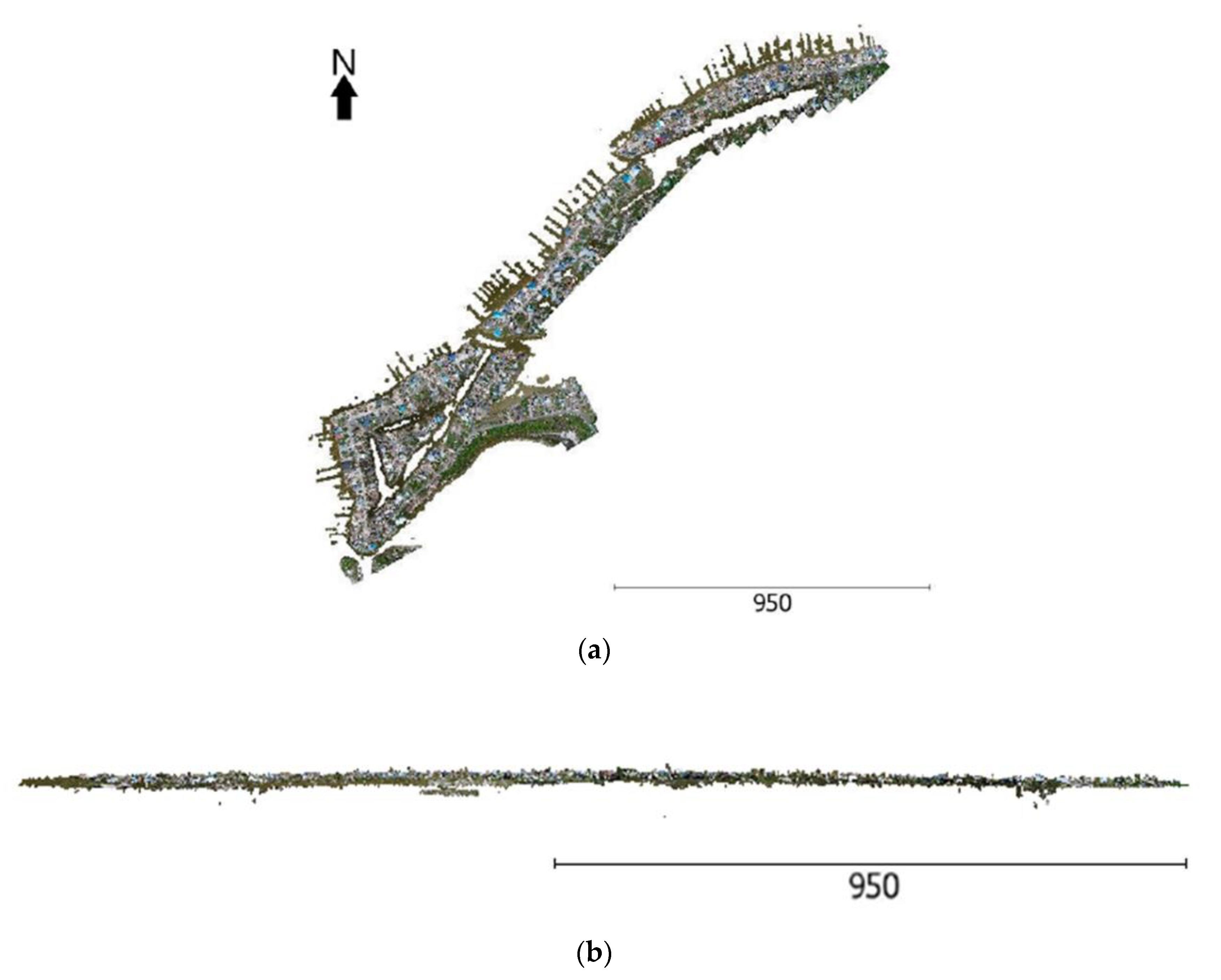
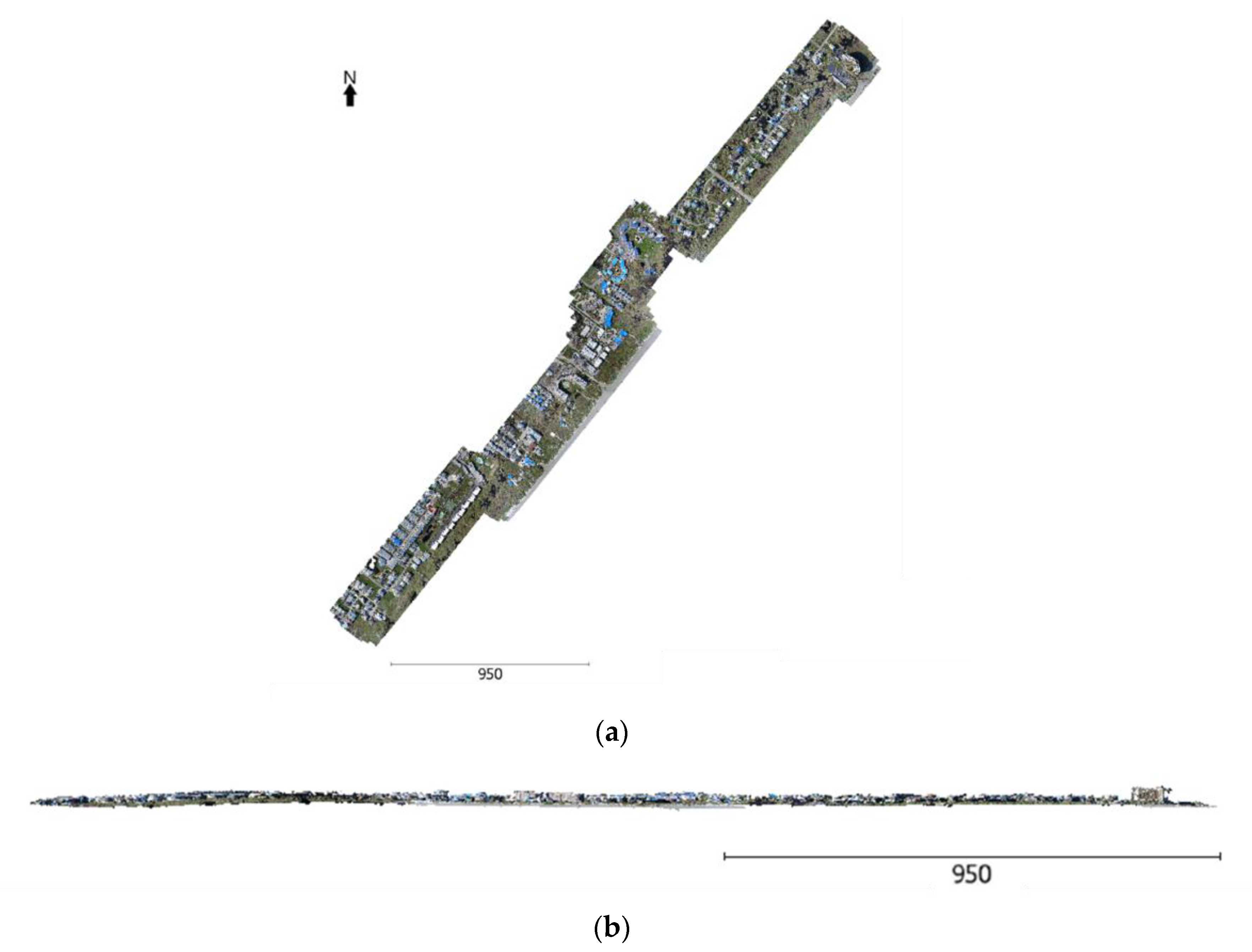
3. Datasets
3.1. Introduction to Hurricane Harvey and Maria
3.2. Data Collection Method
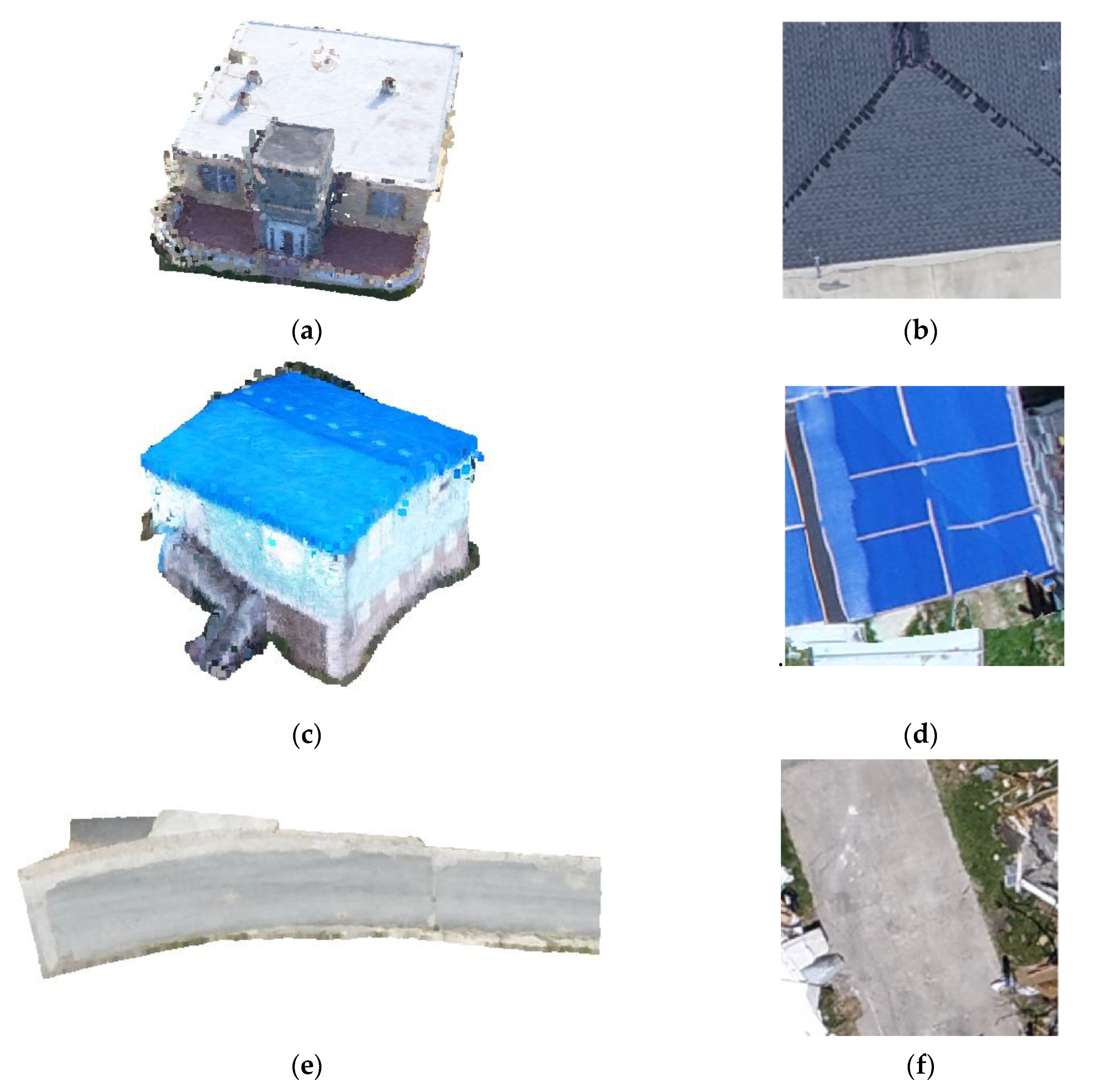
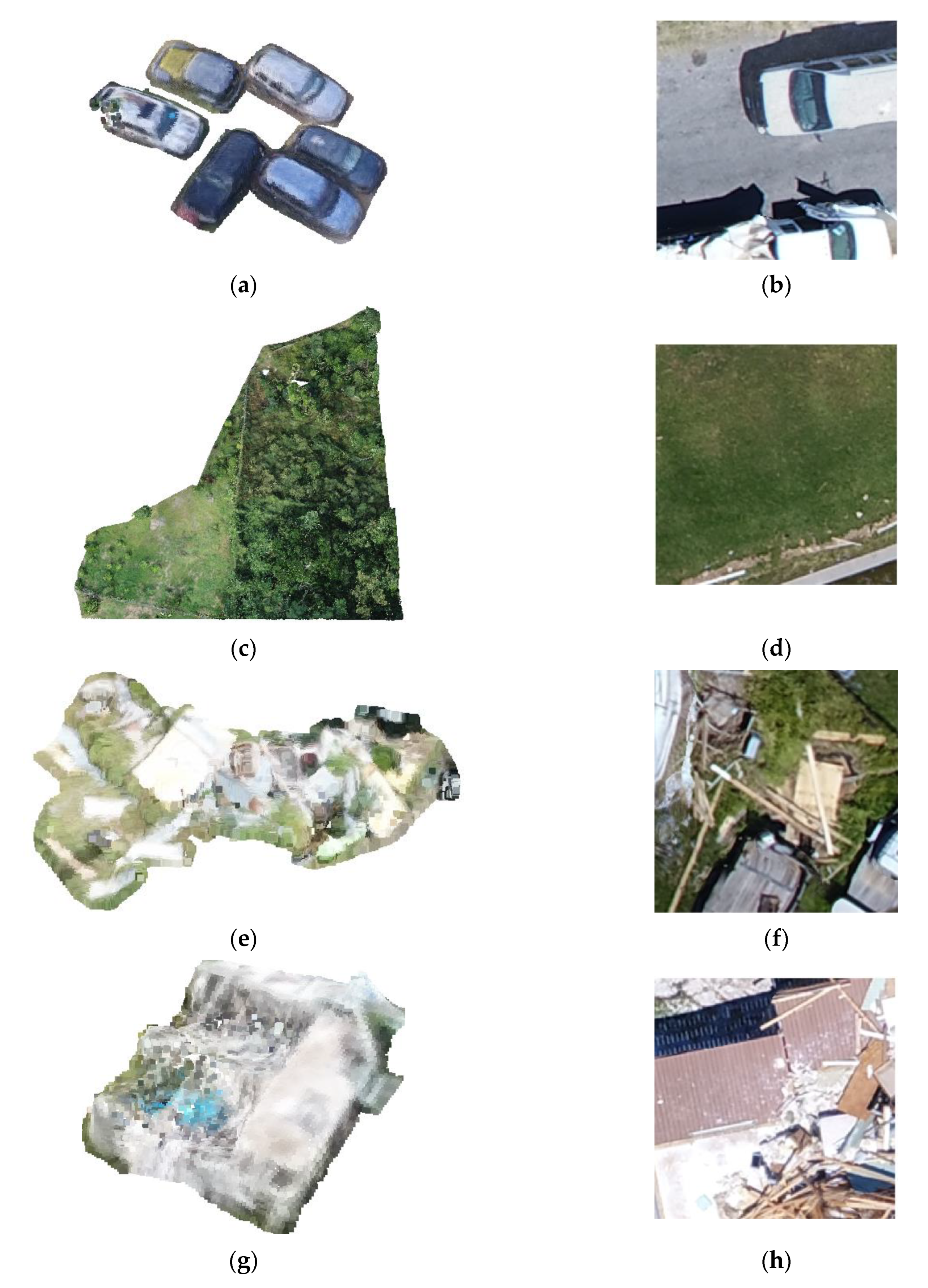
3.3. Dataset Classes
4. Methodology
4.1. Dataset Preparation for 2D Images
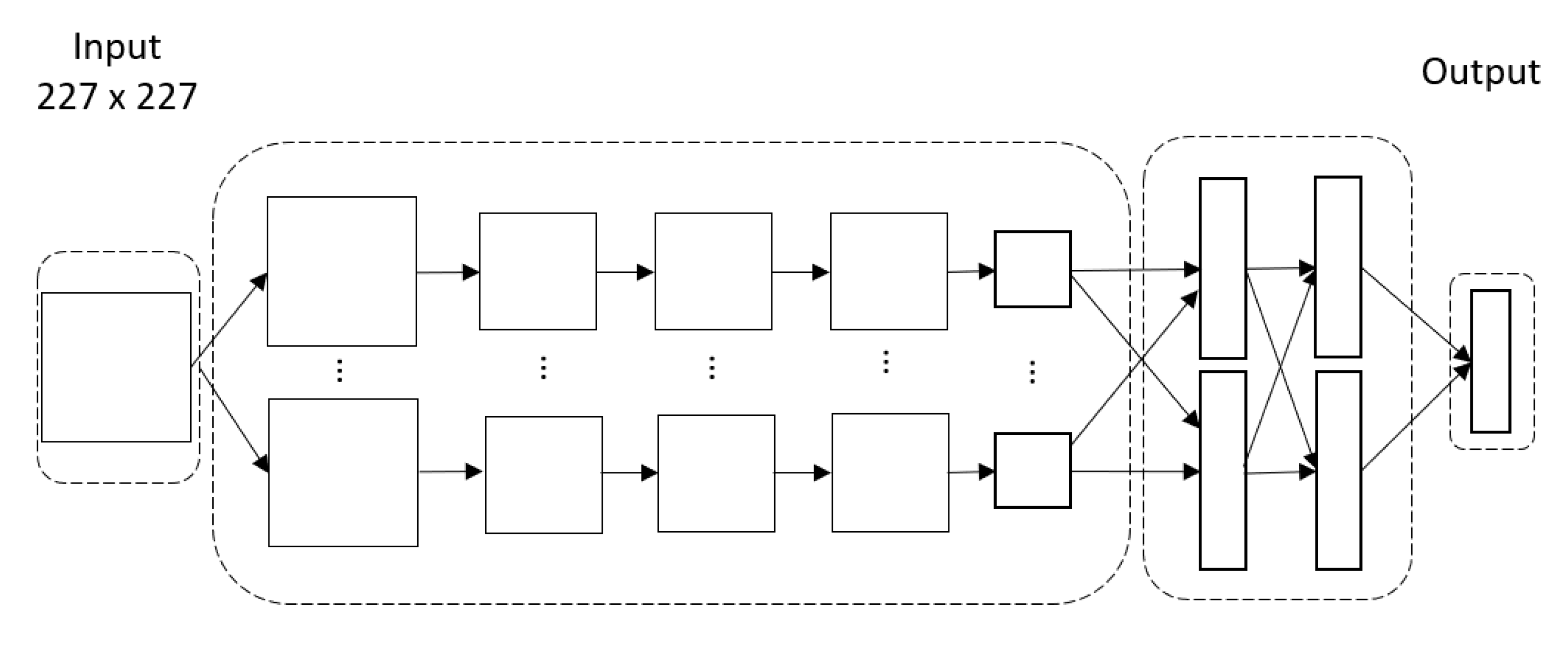
4.2. 2D Convolutional Neural Network Architecture
4.3. Dataset Preparation for 3D Point Clouds
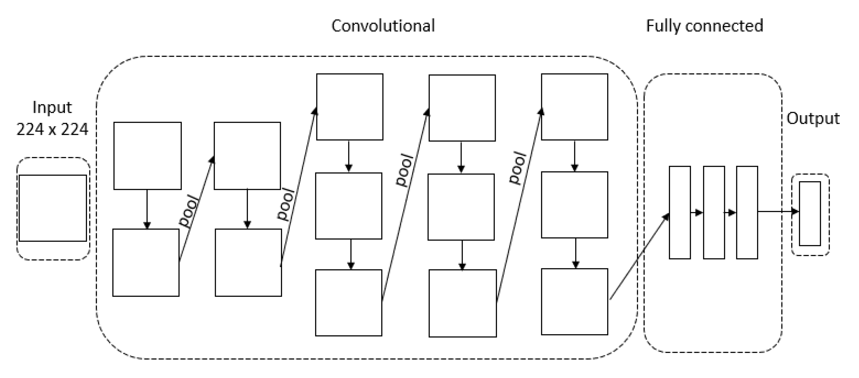
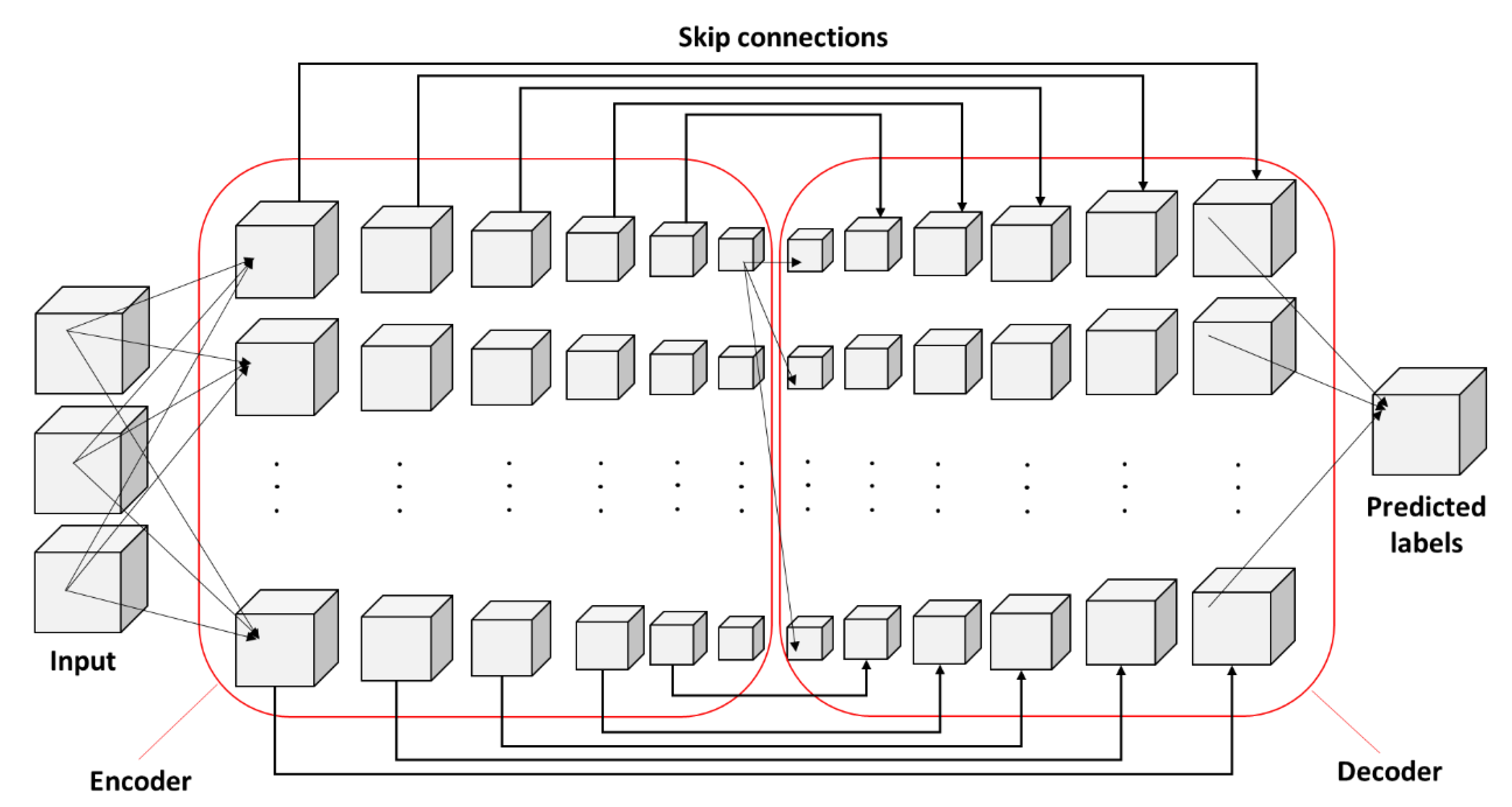
4.4. 3D Fully Convolutional Network Architecture with Skip Connections
5. Discussion
5.1. 2D CNN Experiment
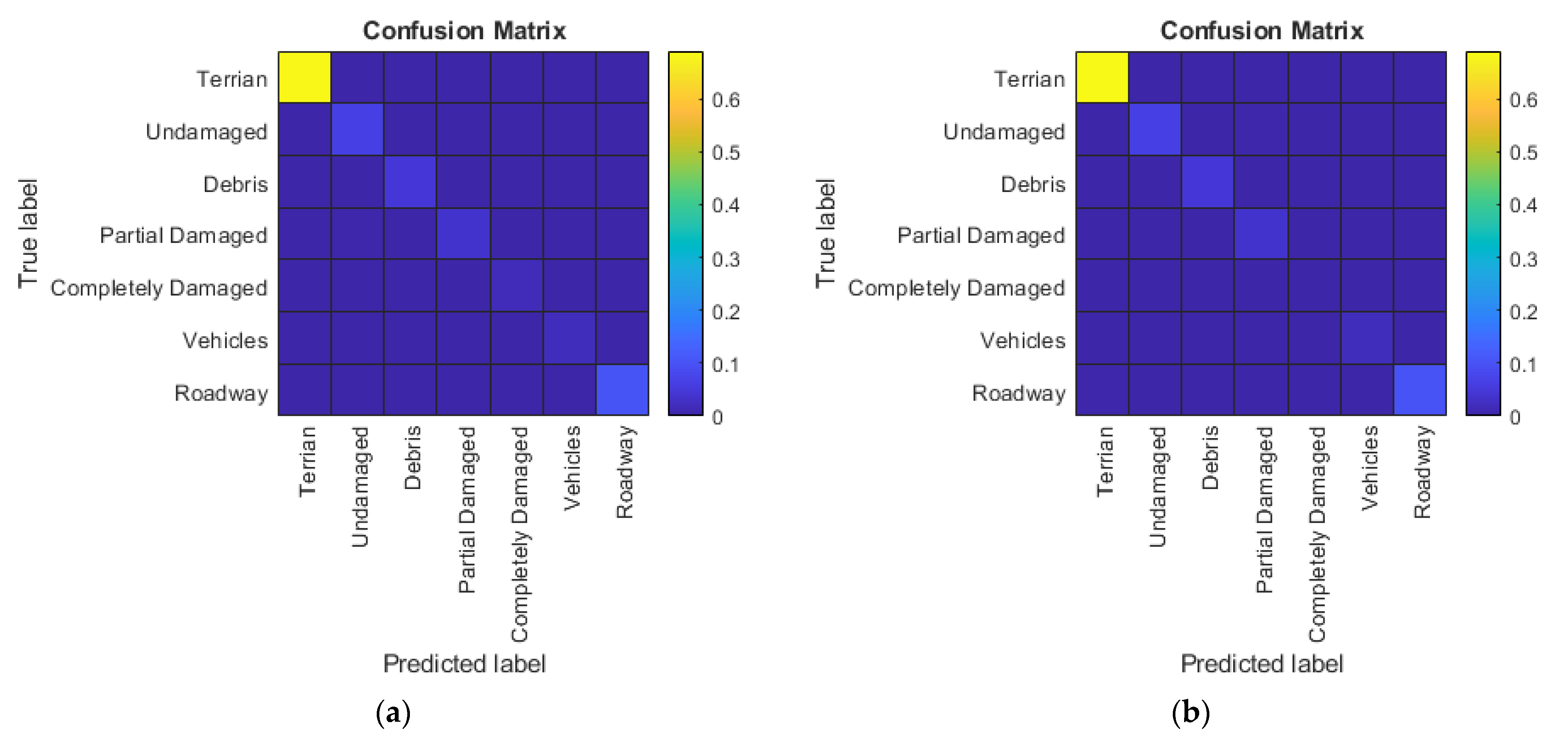
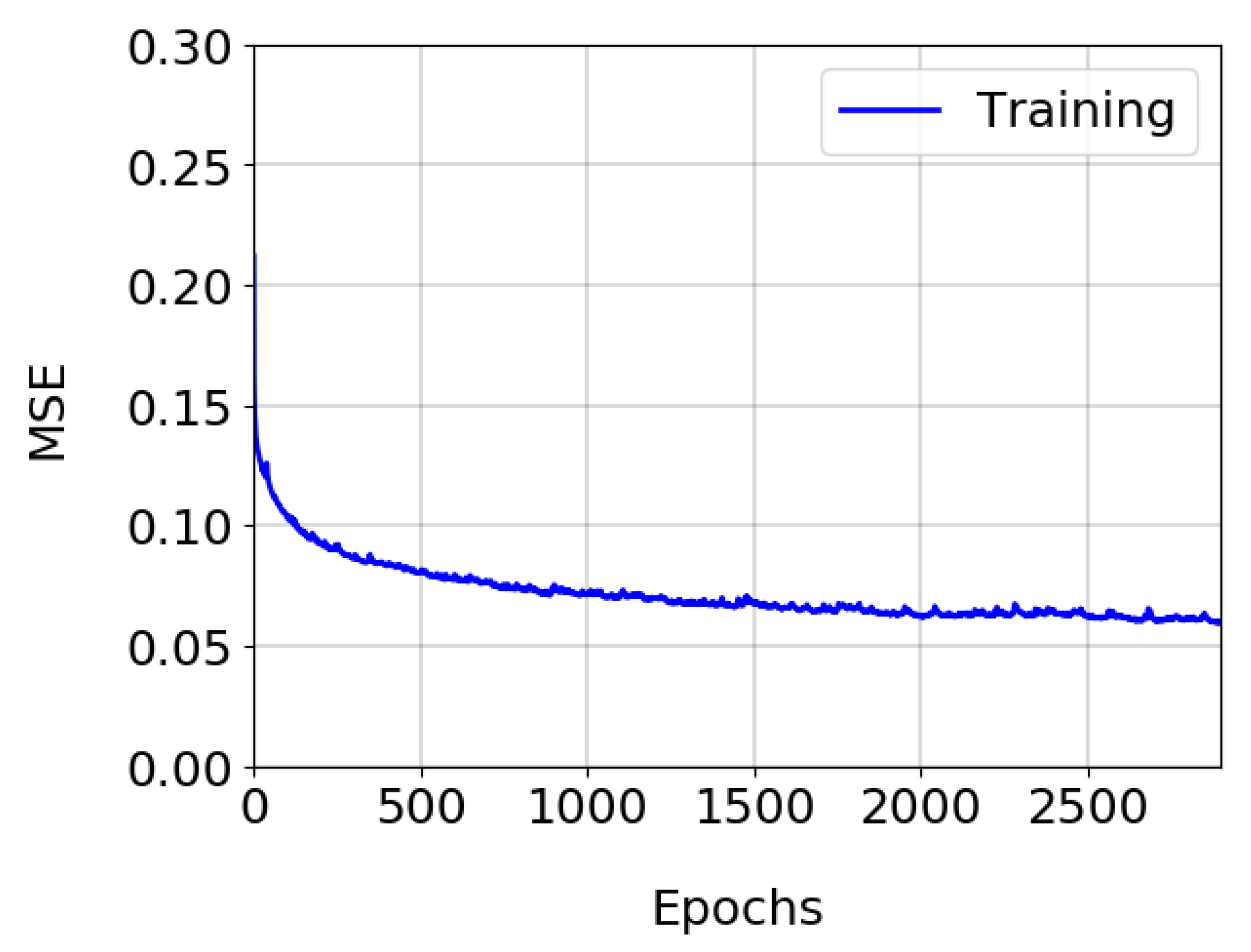
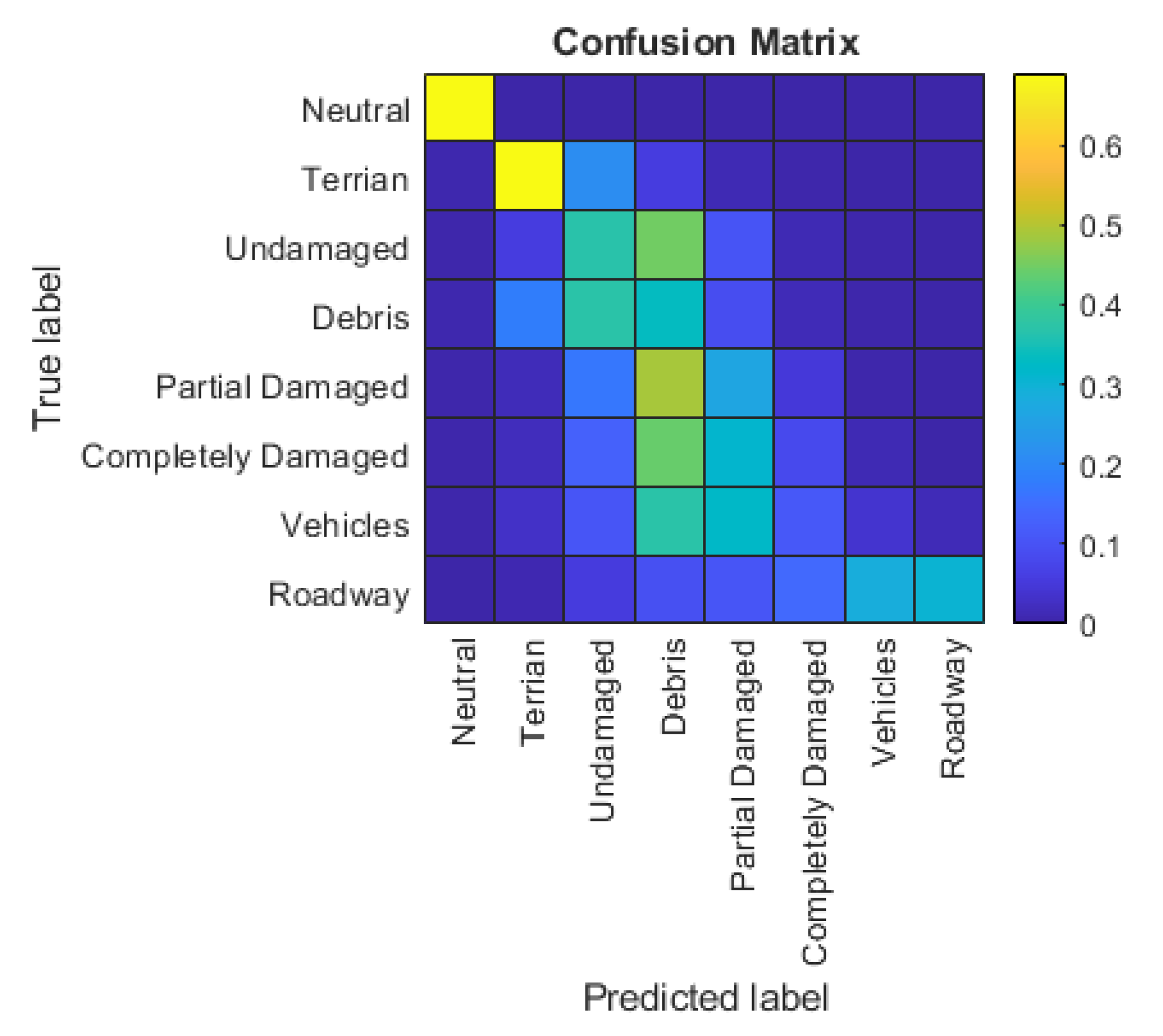
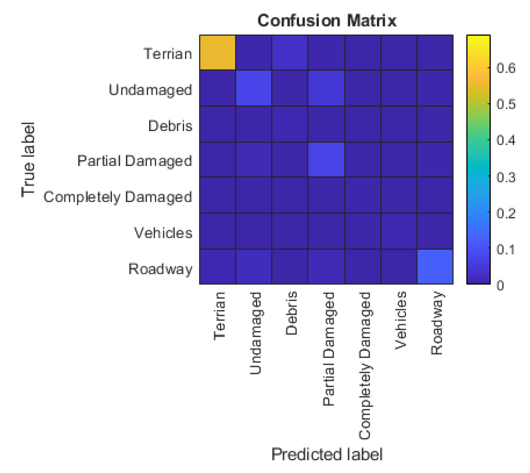
5.2. 3D FCN Experiment
5.3. Comparison of 2D CNN and 3D FCN
6. Conclusions
Author Contributions
Funding
Acknowledgments
Conflicts of Interest
References
- Liao, Y.; Wood, R.L.; Mohammadi, M.E.; Hughes, P.J.; Womble, J.A. Investigation of Rapid Remote Sensing Techniques for Forensic Wind Analyses, 5th, ed.; American Association for Wind Engineering Workshop: Miami, FL, USA, 2018. [Google Scholar]
- Adams, S.M.; Levitan, M.L.; Friedland, C.J. High resolution imagery collection utilizing unmanned aerial vehicles (UAVs) for post-disaster studies. In Advances in Hurricane Engineering: Learning from Our Past; American Society of Civil Engineers: Reston, VA, USA, 2013; pp. 777–793. [Google Scholar]
- Chiu, W.K.; Ong, W.H.; Kuen, T.; Courtney, F. Large structures monitoring using unmanned aerial vehicles. Procedia Eng. 2017, 188, 415–423. [Google Scholar] [CrossRef]
- Zhou, Z.; Gong, J.; Guo, M. Image-based 3D reconstruction for posthurricane residential building damage assessment. J. Comput. Civil Eng. 2016, 30, 04015015. [Google Scholar] [CrossRef]
- Fernandez Galarreta, J.; Kerle, N.; Gerke, M. UAV-based urban structural damage assessment using object-based image analysis and semantic reasoning. Nat. Hazards Earth Syst. Sci. Discuss. 2014, 2, 5603–5645. [Google Scholar] [CrossRef]
- Shin, H.-C.; Roth, H.R.; Gao, M.; Lu, L.; Xu, Z.; Nogues, I.; Yao, J.; Mollura, D.; Summers, R.M. Deep convolutional neural networks for computer-aided detection: CNN architectures, dataset characteristics and transfer learning. IEEE Trans. Med. Imaging 2016, 35, 1285–1298. [Google Scholar] [CrossRef] [PubMed]
- Mohammadi, M.E.; Watson, D.P.; Wood, R.L. Deep Learning-Based Damage Detection from Aerial SfM Point Clouds. Drones 2019, 3, 68. [Google Scholar] [CrossRef]
- Bengio, Y. Deep learning of representations for unsupervised and transfer learning. In Proceedings of ICML Workshop on Unsupervised and Transfer Learning; Workshop and Conference Proceedings: Pittsburgh, PA, USA, 2012; pp. 17–36. [Google Scholar]
- Krizhevsky, A.; Sutskever, I.; Hinton, G.E. Imagenet classification with deep convolutional neural networks. In Proceedings of Advances in Neural Information Processing Systems; Communication of the ACM: Silicon Valley, CA, USA, 2017; pp. 1097–1105. [Google Scholar]
- Berg, A.; Deng, J.; Fei-Fei, L. Large Scale Visual Recognition Challenge. 2010. Available online: http://www.image-net.org/challenges/LSVRC/2010/ (accessed on 1 May 2010).
- Oquab, M.; Bottou, L.; Laptev, I.; Sivic, J. Learning and transferring mid-level image representations using convolutional neural networks. In Proceedings of the IEEE Conference on Computer Vision and Pattern Recognition, Columbus, OH, USA, 23–28 June 2014; pp. 1717–1724. [Google Scholar]
- Hoskere, V.; Narazaki, Y.; Hoang, T.A.; Spencer, B.F., Jr. Towards automated post-earthquake inspections with deep learning-based condition-aware models. arXiv 2018, arXiv:1809.09195. [Google Scholar]
- Xu, Z.; Chen, Y.; Yang, F.; Chu, T.; Zhou, H. A Post-earthquake Multiple Scene Recognition Model Based on Classical SSD Method and Transfer Learning. ISPRS Int. J. Geo-Inf. 2020, 9, 238. [Google Scholar] [CrossRef]
- Simonyan, K.; Zisserman, A. Very deep convolutional networks for large-scale image recognition. arXiv 2014, arXiv:1409.1556. [Google Scholar]
- Gao, Y.; Mosalam, K.M. Deep transfer learning for image-based structural damage recognition. Comput. Aided Civil Infrastruct. Eng. 2018, 33, 748–768. [Google Scholar] [CrossRef]
- Olsen, M.J.; Kayen, R. Post-earthquake and tsunami 3D laser scanning forensic investigations. In Forensic Engineering 2012: Gateway to a Safer Tomorrow; Sixth Congress on Forensic Engineering: San Francisco, CA, USA, 2013; pp. 477–486. [Google Scholar]
- Womble, J.A.; Wood, R.L.; Mohammadi, M.E. Multi-scale remote sensing of tornado effects. Front. Built Environ. 2018, 4, 66. [Google Scholar] [CrossRef]
- Aixia, D.; Zongjin, M.; Shusong, H.; Xiaoqing, W. Building damage extraction from post-earthquake airborne LiDAR data. Acta Geol. Sin. -Engl. Ed. 2016, 90, 1481–1489. [Google Scholar] [CrossRef]
- Hackel, T.; Wegner, J.D.; Schindler, K. Fast Semantic Segmentation of 3d Point Clouds with Strongly Varying Density. Int. Arch. Photogramm 2016, 3, 177–184. [Google Scholar] [CrossRef]
- Xing, X.-F.; Mostafavi, M.A.; Edwards, G.; Sabo, N. An improved automatic pointwise semantic segmentation of a 3D urban scene from mobile terrrstrial and airborne lidar point clouds: a mechine learning approach. ISPRS Ann. Photogramm. Remote Sens. Spat. Inf. Sci. 2019, 4. [Google Scholar]
- Prokhorov, D. A convolutional learning system for object classification in 3-D lidar data. IEEE Trans. Neural Netw. 2010, 21, 858–863. [Google Scholar] [CrossRef]
- Weng, J.; Luciw, M. Dually optimal neuronal layers: Lobe component analysis. IEEE Trans. Auton. Ment. Dev. 2009, 1, 68–85. [Google Scholar] [CrossRef]
- Maturana, D.; Scherer, S. Voxnet: A 3d convolutional neural network for real-time object recognition. In Proceedings of the 2015 IEEE/RSJ International Conference on Intelligent Robots and Systems (IROS), Hamburg, Germany, 28 September–2 October 2015; pp. 922–928. [Google Scholar]
- Hackel, T.; Savinov, N.; Ladicky, L.; Wegner, J.D.; Schindler, K.; Pollefeys, M. Semantic3d. net: A new large-scale point cloud classification benchmark. arXiv 2017, arXiv:1704.03847. [Google Scholar]
- Zhang, F.; Guan, C.; Fang, J.; Bai, S.; Yang, R.; Torr, P.; Prisacariu, V. Instance segmentation of lidar point clouds. ICRA Cited 2020, 4. [Google Scholar]
- Blake, E.S.; Zelinsky, D.A. National Hurricane Center Tropical Cyclone Report: Hurricane Harvey; National Hurricane Center, National Oceanographic and Atmospheric Association: Washington, DC, USA, 2018.
- Smith, A.; Lott, N.; Houston, T.; Shein, K.; Crouch, J.; Enloe, J. US Billion-Dollar Weather and Climate Disasters 1980–2018; National Oceanic and Atmospheric Administration: Washington, DC, USA, 2018.
- Pasch, R.J.; Penny, A.B.; Berg, R. National Hurricane Center Tropical Cyclone Report: Hurricane Maria; Tropical Cyclone Report Al152017; National Oceanic And Atmospheric Administration and the National Weather Service: Washington, DC, USA, 2018; pp. 1–48.
- ASCE (American Society of Civil Engineers). Minimum design loads and associated criteria for buildings and other structures. ASCE standard ASCE/SEI 7–16. Available online: https://ascelibrary.org/doi/book/10.1061/9780784414248 (accessed on 1 May 2019).
- Beale, M.H.; Hagan, M.T.; Demuth, H.B. Neural Network Toolbox™ User’s Guide; The MathWorks: Natick, MA, USA, 2010. [Google Scholar]
- Srivastava, N.; Hinton, G.; Krizhevsky, A.; Sutskever, I.; Salakhutdinov, R. Dropout: a simple way to prevent neural networks from overfitting. J. Mach. Learn. Res. 2014, 15, 1929–1958. [Google Scholar]
- Ghazi, M.M.; Yanikoglu, B.; Aptoula, E. Plant identification using deep neural networks via optimization of transfer learning parameters. Neurocomputing 2017, 235, 228–235. [Google Scholar] [CrossRef]
- Long, J.; Shelhamer, E.; Darrell, T. Fully convolutional networks for semantic segmentation. In Proceedings of the IEEE Conference on Computer Vision and Pattern Recognition, Boston, MA, USA, 7–12 June 2015; pp. 3431–3440. [Google Scholar]
- Ronneberger, O.; Fischer, P.; Brox, T. U-net: Convolutional networks for biomedical image segmentation. In Proceedings of the International Conference on Medical Image Computing and Computer-Assisted Intervention, Munich, Germany, 5–9 October 2015; pp. 234–241. [Google Scholar]


| Dataset | Characteristics | ||
|---|---|---|---|
| GSD (cm) | Orthomosaic Dimensions (pixels) | Point Cloud Number of Vertices (count) | |
| Puerto Rico | 1.09 | 29,332 × 39,482 | 393,764,295 |
| Texas – Salt Lake | 2.73 | 61,395 × 61,937 | 78,830,950 |
| Texas – Port Aransas | 2.69 | 96,216 × 84,611 | 131,902,480 |
| Instance | Number of Instances | ||
|---|---|---|---|
| Texas-Salt Lake | Puerto Rico | Texas-Port Aransas | |
| Terrain | 719 | 224 | 665 |
| Undamaged Structure | 307 | 97 | 355 |
| Debris | 404 | 764 | 257 |
| Partially Damaged Structure | 99 | 76 | 115 |
| Completely Damaged Structure | 146 | 364 | 76 |
| Vehicle | 256 | 198 | 224 |
| Roadway | 57 | 166 | 87 |
| Instance | Number of Instances | ||
|---|---|---|---|
| Texas-Salt Lake | Puerto Rico | Texas-Port Aransas | |
| Terrain | 1972 | 5238 | 3288 |
| Undamaged Structure | 138 | 610 | 688 |
| Debris | 296 | 247 | 71 |
| Partially Damaged Structure | 236 | 223 | 485 |
| Completely Damaged Structure | 152 | 74 | 33 |
| Vehicle | 67 | 160 | 53 |
| Roadway | 246 | 864 | 904 |
| Classes | 3D FCN | |
|---|---|---|
| Precision | Recall | |
| Neutral | 100 | 100 |
| Terrain | 85 | 70 |
| Undamaged Structure | 15 | 37 |
| Debris | 31 | 33 |
| Partially Damaged Structure | 8 | 26 |
| Completely Damaged Structure | 14 | 8 |
| Vehicle | 4 | 4 |
| Roadway | 94 | 94 |
| Classes | 3D FCN | |
|---|---|---|
| Precision | Recall | |
| Neutral | 100 | 100 |
| Terrain | 61 | 31 |
| Undamaged Structure | 12 | 28 |
| Debris | 3 | 40 |
| Partially Damaged Structure | 10 | 29 |
| Completely Damaged Structure | 1 | 4 |
| Vehicle | 1 | 2 |
| Roadway | 95 | 13 |
© 2020 by the authors. Licensee MDPI, Basel, Switzerland. This article is an open access article distributed under the terms and conditions of the Creative Commons Attribution (CC BY) license (http://creativecommons.org/licenses/by/4.0/).
Share and Cite
Liao, Y.; Mohammadi, M.E.; Wood, R.L. Deep Learning Classification of 2D Orthomosaic Images and 3D Point Clouds for Post-Event Structural Damage Assessment. Drones 2020, 4, 24. https://doi.org/10.3390/drones4020024
Liao Y, Mohammadi ME, Wood RL. Deep Learning Classification of 2D Orthomosaic Images and 3D Point Clouds for Post-Event Structural Damage Assessment. Drones. 2020; 4(2):24. https://doi.org/10.3390/drones4020024
Chicago/Turabian StyleLiao, Yijun, Mohammad Ebrahim Mohammadi, and Richard L. Wood. 2020. "Deep Learning Classification of 2D Orthomosaic Images and 3D Point Clouds for Post-Event Structural Damage Assessment" Drones 4, no. 2: 24. https://doi.org/10.3390/drones4020024
APA StyleLiao, Y., Mohammadi, M. E., & Wood, R. L. (2020). Deep Learning Classification of 2D Orthomosaic Images and 3D Point Clouds for Post-Event Structural Damage Assessment. Drones, 4(2), 24. https://doi.org/10.3390/drones4020024