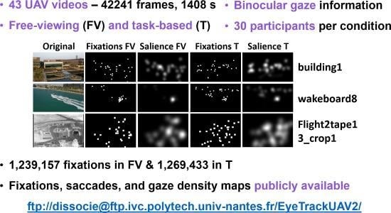
EyeTrackUAV2: A Large-Scale Binocular Eye-Tracking Dataset for UAV Videos

Abstract

The fast and tremendous evolution of the unmanned aerial vehicle (UAV) imagery gives place to the multiplication of applications in various fields such as military and civilian surveillance, delivery services, and wildlife monitoring. Combining UAV imagery with study of dynamic salience further extends the number of future applications. Indeed, considerations of visual attention open the door to new avenues in a number of scientific fields such as compression, retargeting, and decision-making tools. To conduct saliency studies, we identified the need for new large-scale eye-tracking datasets for visual salience in UAV content. Therefore, we address this need by introducing the dataset EyeTrackUAV2. It consists of the collection of precise binocular gaze information (1000 Hz) over 43 videos (RGB, 30 fps, 1280 × 720 or 720 × 480). Thirty participants observed stimuli under both free viewing and task conditions. Fixations and saccades were then computed with the dispersion-threshold identification (I-DT) algorithm, while gaze density maps were calculated by filtering eye positions with a Gaussian kernel. An analysis of collected gaze positions provides recommendations for visual salience ground-truth generation. It also sheds light upon variations of saliency biases in UAV videos when opposed to conventional content, especially regarding the center bias.

1. Introduction

For a couple of decades now, we have witnessed the fast advances and growing use of UAV for multiple critical applications. UAV refers here to unmanned aerial vehicles, autonomous or monitored from remote sites. This imagery enables a broad range of uses, from making vacation movies to drone races for mainstream civilian applications. Tremendous professional services are developed, among others fire detection [1], wildlife counting [2], journalism [3], precision agriculture, and delivery services. But most applications are military, from aerial surveillance [4], drone-based warfare [5] to moving targets tracking [6], object, person, and anomaly detection [7,8,9].

The UAV imagery proposes a new representation of visual scenes that makes all these new applications possible. UAV vision is dominant and hegemonic [10]. The bird point of view modifies the perspective, size and features of objects [11]. It introduces a loss of pictorial depth cues [12] such as horizontal line [13]. Also, UAV high autonomy in conjunction with large-field of view camera permits to cover large areas in limited time duration. Besides, embedded sensors can be multi-modal and can include RGB, thermal, IR, or multi-spectral sensors. Multiplying imagery modalities allows overcoming possible weaknesses of RGB-only cameras [10]. For instance, occlusions may be compensated by thermal information, and the capture of IR is desired for low-luminance environments [14].

UAV scene depiction is rich, comprehensive, and promising, which explains its success. However, challenges to come are even more compelling. Edney-Browne [10] wondered how the capacity of UAV capturing the external reality (visuality) is related to perceptual and cognitive vision in humans. Variations in UAV characteristics such as perspective view and object size may change viewers’ behavior towards content. Consequently, new visual attention processes may be triggered for this specific imaging. This means that studying UAV imagery in light of human visual attention not only opens the door to plenty of applications but could also enable to gather further knowledge on perceptual vision and cognition.

In the context of UAV content, there are very few eye-tracking datasets. This is the reason why we propose and present in this paper a new large-scale eye-tracking dataset, freely downloadable from the internet. This dataset aims to strengthen our knowledge on human perception and could play a fundamental role for designing new computational models of visual attention.

The paper is organized as follows. In Section 2, we first justify and elaborate on the need for large-scale eye-tracking databases for UAV videos. Then, we introduce the entire process of dataset creation in Section 3. It describes the content selection, the experiment set up, and the implementation of fixations, saccades, and gaze density maps. Section 4 presents an in-depth analysis of the dataset. The study is two-fold: it explores what ground truth should be used for salience studies, and brings to light the fading of conventional visual biases UAV stimuli. Finally, conclusions are provided in Section 5.

2. Related Work

Visual attention occurs to filter and sort out visual clues. Indeed, it is impossible to process simultaneously all the information of our visual field. Particular consideration should be dedicated to identifying which attentional processes are involved as they are diverse and aim at specific behaviors. For instance, one must make the distinction between overt and covert attention [15]. The former refers to a direct focus where eyes and head point. The latter relates to the peripheral vision, where attention is directed without eye movement towards it. In practice, when an object of interest is detected in the area covered by the covert attention, one may make a saccade movement to direct the eyes from the overt area to this position. The context of visualization is also important. For instance, we make a distinction between two content exploration processes [16]: (1) A no constraint examination named free viewing. The observer is rather free from cognitive loads and is supposed to mainly use bottom-up or exogenous attention processes driven by external factors, e.g., content and environment stimuli. (2) A task-based visualization, such as surveillance for instance. Cognitive processes such as prior knowledge, wilful plans, and current goals guide the viewer’s attention. This is known as top-down or endogenous attention. A strict division is slightly inaccurate in that both top-down and bottom-up processes are triggered during a visual stimuli in a very intricate interaction [17,18].

In computer science, it is common to study bottom-up and top-down processes through the visual salience. Visual salience is a representation of visual attention in multimedia content as a probability distribution per pixels [19]. Salience analyses rest on the relation of visual attention to eye movements, and these latter are obtained through gaze collection with eye-trackers [20]. Saliency predictions help to understand computational cognitive neuroscience as it reveals attentional behaviors and systematic viewing tendencies such as center bias [17]. Multiple applications derive from saliency predictions such as compression [21], content-aware re-targeting, object segmentation [22], and detection [23,24].

Recently, there has been a growing interest on one particular application, which combines visual salience and UAV content. Information overload in the drone program and fatigue in military operators may have disastrous consequences for military applications [10]. New methods and approaches are required to detect anomaly in UAV footages and to ease the decision-making. Among them, we believe that computational models of visual attention could be used to simulate operators’ behaviors [25]. Eventually, thanks to predictions, operators’ workloads can be reduced by eliminating unnecessary footages segments. Other works support the use of salience to enhance the efficiency of target-detection task completion. For instance Brunyé et al. [26] studied the combination of salience (in terms of opacity with the environment) and biological motion (presence and speed) in textured backgrounds. They concluded that salience is very important for slowly moving objects, such as camouflaged entities. Meanwhile, fast biological movements are highly attention-grabbing, which diminishes the impact of static salience. Accordingly, it makes sense to develop dynamic saliency models tailored to UAV content.

However, we demonstrate in [27] that current saliency models lack efficiency in terms of prediction for UAV content. This applies to all types of prediction models, handcrafted features and architecture implementing deep learning to a lesser extent, whether they are static or dynamic schemes. Typical handcrafted and low-level features learnt on conventional imaging may not suit UAV content. Besides, in conventional imaging the center position is the best location to have access to most visual information of a content [28]. This fact leads to a well-known bias in visual attention named central bias. This effect may be associated with various causes. For instance, Tseng et al. [29] showed a contribution of photographer bias, viewing strategy, and to a lesser extent, motor, re-centering, and screen center biases to the center bias. They are briefly described below:

• The photographer bias often emphasizes objects in the content center through composition and artistic intent [29].
• Directly related to photographer bias, observers tend to learn the probability of finding salient objects at the content center. We refer to this behavior as a viewing strategy.
• With regards to the human visual system (HVS), the central orbital position, that is when looking straight ahead, is the most comfortable eye position [30], leading to a recentering bias.
• Additionally, there is a motor bias, in which one prefers making short saccades and horizontal displacements [31,32].
• Lastly, onscreen presentation of visual content pushes observers to stare at the center of the screen frame [28,33]. This experimental bias is named the screen center bias.

The central bias is so critical in the computational modelling of visual attention that saliency models include this bias as prior knowledge or use it as a baseline to which saliency predictions are being compared [34]. The center bias is often represented by a centered isotropic Gaussian stretched to the video frame aspect ratio [35,36]. The presence of this bias in UAV videos has already been questioned in our previous work [27]. We showed that saliency models that heavily rely on the center bias were less efficient on Unmanned Aerial Vehicle (UAV) videos than on conventional video sequences. Therefore, we believe that the central bias could be less significant in drone footage as a result of the lack of photographer bias or due to UAV content characteristics. It would be beneficial to evaluate qualitatively and quantitatively the center bias on a larger dataset of UAV videos to support our assumption.

While it is now rather easy to find eye tracking data on typical images [35,37,38,39,40,41,42,43,44,45] or videos [46,47,48,49,50], and that there are many UAV content datasets [7,51,52,53,54,55,56,57,58,59,60,61,62], it turns out to be extremely difficult to find eye-tracking data on UAV content. This is even truer when we consider dynamic salience, which refers to salience for video content. To the best of our knowledge, EyeTrackUAV1 dataset released in 2018 [11] is the only public dataset available for studying the visual deployment over UAV video. There exists another dataset AVS1K [63]. However, AVS1K is, to the present day, not publicly available. We thus focus here on EyeTrackUAV1, with the awareness that all points below but the last apply to AVS1K.

EyeTrackUAV1 consists of 19 sequences (1280 × 720 and 30 fps) extracted from the UAV123 database [55]. The sequence selection relied on content characteristics, which are the diversity of environment, distance and angle to the scene, size of the principal object, and the presence of sky. Precise binocular gaze data (1000 Hz) of 14 observers were recorded under free viewing condition, for every content. Overall, the dataset comprises eye-tracking information on 26,599 frames, which represents 887 seconds of video. In spite of a number of merits, this dataset presents several limitations for saliency prediction applications. These limitations have been listed in [27]. We briefly summarize them below:

• UAV may embed multi-modal sensors during the capture of scenes. Besides conventional RGB cameras, to name but a few thermal, multi-spectral, and infrared cameras consist of typical UAV sensors. Unfortunately, EyeTrackUAV1 lacks non-natural content, which is of great interest for the dynamic field of salience. As already mentioned, combining content from various imagery in datasets is advantageous for numerous reasons. It is necessary to continue efforts toward the inclusion of more non-natural content in databases.
• In general, the inclusion of more participants in the collection of human gaze is encouraged. Indeed, reducing variable errors by including more participants in the eye tracking experiment is beneficial. It is especially true in the case of videos as salience is sparse due to the short displaying duration of a single frame. With regards to evaluation analyses, some metrics measuring similarity between saliency maps consider fixation locations for saliency comparison (e.g., any variant of area under the curve (AUC), normalized scanpath saliency (NSS), and information gain (IG)). Having more fixation points is more convenient for the use of such metrics.
• EyeTrackUAV1 contains eye-tracking information recorded during free-viewing sessions. That is, no specific task was assigned to observers. Several applications for UAV and conventional imaging could benefit from the analysis and reproduction of more top-down attention, related to a task at hand. More specifically, for UAV content, there is a need for specialized computational models for person or anomaly detection.
• Even though there are about 26,599 frames in EyeTrackUAV, they come from only 19 videos. Consequently, this dataset just represents a snapshot of the reality. We aim to go further by introducing more UAV content.

To extend and complete the previous dataset and to tackle these limitations, we have created the EyeTrackUAV2 dataset, introduced below.

3. EyeTrackUAV2 Dataset

This section introduces the new dataset EyeTrackUAV2 aiming at tackling issues mentioned above. EyeTrackUAV2 includes more video content than its predecessor EyeTrackUAV1. It involves more participants, and considers both free and task-based viewing. In the following subsections, we first elaborate on the selection of video content, followed by a description of the eye-tracking experiment. It includes the presentation of the eye-tracking apparatus, the experiment procedure and setup, and the characterization of population samples. Finally, we describe the generation of the human ground truth, i.e., algorithms for fixation and saccade detection as well as gaze density map computation.

3.1. Content Selection

Before collecting eye-tracking information, experimental stimuli were selected from multiple UAV video datasets. We paid specific attention to select videos suitable for both free and task-based viewing as experimental conditions. Also, the set of selected videos had to cover multiple UAV flight altitudes, main surrounding environments, main sizes of observed objects and angles between the aerial vehicle and the scene, as well as the presence or not of sky. We consider these characteristics favor the construction of a representative dataset of typical UAV videos, as suggested in [11].

We examined the following UAV datasets: UCF’s dataset (http://crcv.ucf.edu/data/UCF_Aerial_Action.php), VIRAT [51], MRP [52], the privacy-based mini-drones dataset [53], the aerial videos dataset described in [54], UAV123 [55], DTB70 [57], Okutama-Action [58], VisDrone [64], CARPK [59], SEAGULL [60], DroneFace [61], and the aerial video dataset described in [56]). A total of 43 videos (RGB, 30 frame per second (fps), 1280 × 720 or 720 × 480) were selected from databases VIRAT, UAV123, and DTB70. These three databases exhibited different contents for various applications, which made the final selection representative of the UAV ecosystem. We present below the main characteristics of the three selected datasets:

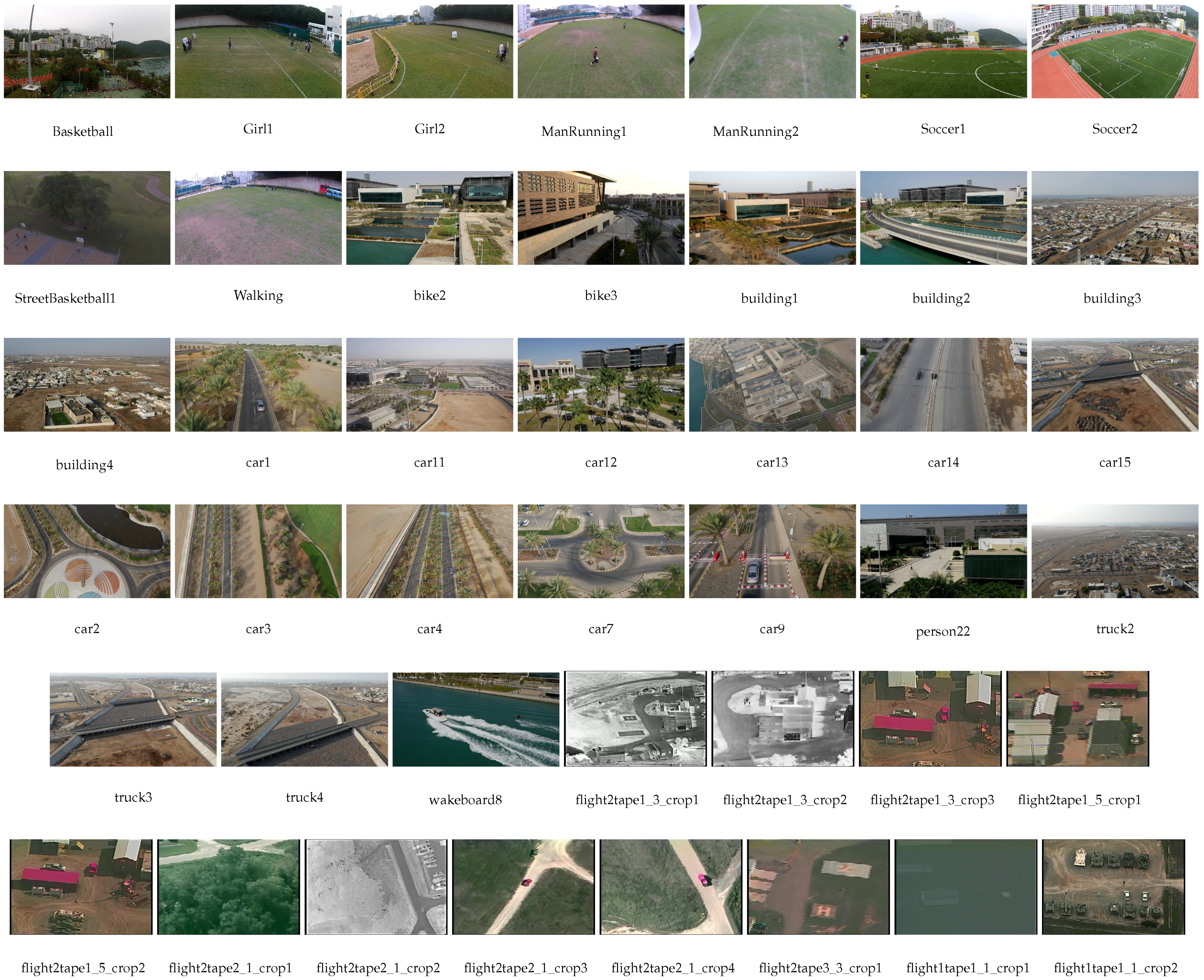
• UAV123 included challenging UAV content annotated for object tracking. We restricted the content selection to the first set, which included 103 sequences (1280 × 720 and 30 fps) captured by an off-the-shelf professional-grade UAV (DJI S1000) tracking various objects in a range of altitudes comprised between 5–25 m. Sequences included a large variety of environments (e.g., urban landscapes, roads, and marina), objects (e.g., cars, boats, and persons) and activities (e.g., walking, biking, and swimming) as well as presenting many challenges for object tracking (e.g., long- and short-term occlusions, illumination variations, viewpoint change, background clutter, and camera motion).
• Aerial videos in the VIRAT dataset were manually selected (for smooth camera motion and good weather conditions) from rushes of a total amount of 4 h in outdoor areas with broad coverage of realistic scenarios for real-world surveillance. Content included “single person”, “person and vehicle”, and “person and facility” events, with changes in viewpoints, illumination, and visibility. The dataset came with annotations of moving object tracks and event examples in sequences. The main advantage of VIRAT videos was its perfect fit for military applications. It covered fundamental environment contexts (events), conditions (rather poor quality and weather condition impairments), and imagery (RGB and IR). We decided to keep the original resolution of videos (720 × 480) to prevent the introduction of unrelated artifacts.
• The 70 videos (RGB, 1280 × 720 and 30 fps) from DTB70 dataset were manually annotated with bounding boxes for tracked objects. Sequences were shot with a DJI Phantom 2 Vision+ drone or were collected from YouTube to add diversity in environments and target types (mostly humans, animals, and rigid objects). There was also a variety of camera movements (both translation and rotation), short- and long-term occlusions, and target deformability.

Table 1. Stimuli original datasets.

Dataset	Native Resolution	Proportion of Content Seen Per Degree of Visual Angle (%)	Videos Number	Frames Number (30 fps)	Duration (s)
VIRAT [51]	720 × 480	1.19	12	17,851	595.03
UAV123 [55]	1280 × 720	0.44	22	20,758	691.93
DTB70 [57]	1280 × 720	0.44	9	3632	121.07
Overall			43	42,241	1408.03 (23:28 min)

reports for each database the number of sequences selected, their native resolution, duration and frame number.

Table 2. Basic statistics on selected videos.

	Number of Frames				Duration (MM:SS)
	VIRAT	UAV123	DTB70	Overall	VIRAT	UAV123	DTB70	Overall
Total	17,851	20,758	3632	42,241	09:55	11:32	02:01	23:28
Average	1488	944	404	982	00:50	00:31	00:13	00:33
Standard Deviation	847	615	177	727	00:28	00:21	00:06	00:24
Minimum	120	199	218	120	00:04	00:07	00:07	00:04
Maximum	3178	2629	626	3178	01:46	01:28	00:21	01:46

presents basic statistics of the database in terms of number of frames and duration.

3.2. Content Diversity

Figure 1 presents the diversity of selected UAV sequences by illustrating the first frame of every content. Visual stimuli cover a variety of visual scenes in different environments (e.g., public and military environments, roads, buildings, sports, port areas, etc.) and different moving or fixed objects (e.g., people, groups of people, cars, boats, bikes, motorbikes, etc.). Selected videos were captured from various flight heights and different angles between the UAV and the ground (allowing or not the presence of sky during their observation). Also, three sequences, extracted from the VIRAT dataset, were captured by IR cameras. Additionally, we considered various video duration as the length of the video may possibly impact the behavior of observers due to fatigue, resulting in a lack of attention and more blinking artifacts [10,65].

To quantitatively show the diversity of selected videos, we have computed temporal and spatial complexity [66], named temporal index (TI) ($\in \left[0,+\infty \right[$) and spatial index (SI) ($\in \left[0,+\infty \right[$), respectively. These features are commonly used in image quality domain for describing the properties of selected images. They characterize the maximum standard deviation of spatial and temporal discrepancies over the entire sequence. The higher a measure is, the more complex the content. TI and SI are reported per sequence in

Table 3. Stimuli ID and name, their original dataset, number of frames together with starting and ending frame number, duration, and native resolution.

ID	Video	Dataset	Number of Frames	Start Frame	End Frame	Duration (ms)	SI	TI	Altitude	Environment	Object Size	Horizontal Line (Sea, Sky)	Main Angle
1	09152008flight2tape1_3 (crop 1)	VIRAT	120	1	120	4000	0.455	32	High	Urban military - IR	Small	False	Oblique
2	09152008flight2tape1_3 (crop 2)		367	137	503	12,234	0.474	35	High	Urban military - IR	Small	False	Oblique
3	09152008flight2tape1_3 (crop 3)		3178	4735	7912	105,934	0.452	43	Intermediate	Urban military	Medium, Small	False	Oblique
4	09152008flight2tape1_5 (crop 1)		972	218	1189	32,400	0.467	37	Intermediate	Urban military	Medium, Small	False	Oblique
5	09152008flight2tape1_5 (crop 2)		1715	4555	6269	57,167	0.461	45	Intermediate	Urban military	Medium, Small	False	Oblique
6	09152008flight2tape2_1 (crop 1)		1321	1	1321	44,034	0.484	40	Intermediate, Low	Urban military	Medium, Big	False	Oblique
7	09152008flight2tape2_1 (crop 2)		1754	2587	4340	58,467	0.484	41	High	Roads rural - IR	Small	False	Oblique
8	09152008flight2tape2_1 (crop 3)		951	4366	5316	31,700	0.482	33	Intermediate	Urban military	Medium, Big	False	Oblique
9	09152008flight2tape2_1 (crop 4)		1671	6482	8152	55,700	0.452	32	High	Roads rural	Medium	False	Oblique, Vertical
10	09152008flight2tape3_3 (crop 1)		2492	3067	5558	83,067	0.474	42	Intermediate	Urban military	Small	False	Oblique
11	09162008flight1tape1_1 (crop 1)		1894	1097	2990	63,134	0.448	39	Low	Urban military, Roads rural	Medium, Small	False	Oblique
12	09162008flight1tape1_1 (crop 2)		1416	4306	5721	47,200	0.477	29	Intermediate, High	Urban military	Small	False	Oblique
	Average		1488			50,000	0.468	37.33
	Standard deviation		847			28,000	0.01	5.10
13	bike2	UAV123	553	1	553	18,434	0.468	22	Intermediate	Urban, building	Small, Very small	True	Horizontal
14	bike3		433	1	433	14,434	0.462	19	Intermediate	Urban, building	Small	True	Horizontal
15	building1		469	1	469	15,634	0.454	12	Intermediate	Urban, building	Very Small	True	Horizontal
16	building2		577	1	577	19,234	0.471	37	Intermediate	Urban, building	Medium, Small	True	Horizontal
17	building3		829	1	829	27,634	0.451	27	High	Urban in desert	Small	True	Horizontal
18	building4		787	1	787	26,234	0.464	29	High, Intermediate	Urban in desert	None	True, False	Horizontal, Oblique
19	car1		2629	1	2629	87,634	0.471	59	Low, Intermediate	Road rural	Big, Medium	True	Oblique
20	car11		337	1	337	11,234	0.467	31	High	Suburban	Small	True, False	Horizontal, Oblique
21	car12		499	1	499	16,634	0.467	39	Low	Road urban, sea	Medium, Small	True	Horizontal
22	car13		415	1	415	13,834	0.461	26	High	Urban	Very very small	False	Oblique, Vertical
23	car14		1327	1	1327	44,234	0.471	25	Low	Road suburban	Medium	False	Oblique
24	car15		469	1	469	15,634	0.471	18	Intermediate	Road towards urban	Small, Very small	True	Oblique
25	car2		1321	1	1321	44,034	0.464	24	Intermediate	Road rural	Medium	False	Oblique, Vertical
26	car3		1717	1	1717	57,234	0.467	27	Intermediate	Road rural	Medium	False	Oblique, Vertical
27	car4		1345	1	1345	44,834	0.462	23	Intermediate, Low	Road rural	Big	False	Oblique, Vertical
28	car7		1033	1	1033	34,434	0.464	18	Intermediate	Road suburban	Medium	False	Oblique
29	car9		1879	1	1879	62,634	0.470	23	Intermediate, Low	Road suburban	Medium	False, True	Oblique, Horizontal
30	person22		199	1	199	6634	0.456	31	Low	Urban sea	Medium, Big	True	Horizontal
31	truck2		601	1	601	20,034	0.453	24	High	Urban road	Small	True	Horizontal
32	truck3		535	1	535	17,834	0.472	18	Intermediate	Road towards urban	Small, Very small	True	Oblique
33	truck4		1261	1	1261	42,034	0.466	17	Intermediate	Road towards urban	Small	True	Oblique, Horizontal
34	wakeboard8		1543	1	1543	51,434	0.472	39	Low	Sea urban	Medium, Big	True, False	Oblique, Vertical, Horizontal
	Average		944			31,000	0.465	26.73
	Standard deviation		615			21,000	0.01	10.14
35	Basketball	DTB70	427	1	427	14,234	0.477	48	Intermediate	Field suburban	Medium	True	Oblique
36	Girl1		218	1	218	7267	0.481	31	Low	Field suburban	Big	True	Horizontal
37	Girl2		626	1	626	20,867	0.482	30	Low	Field suburban	Big	True	Horizontal
38	ManRunning1		619	1	619	20,634	0.483	23	Low	Field suburban	Big	True	Horizontal, Oblique
39	ManRunning2		260	1	260	8667	0.484	27	Low	Field suburban	Very big	False	Vertical, Oblique
40	Soccer1		613	1	613	20,434	0.476	57	Low, Intermediate	Field suburban	Very big, Big	True	Horizontal
41	Soccer2		233	1	233	7767	0.475	24	High	Field suburban	Small	True	Oblique
42	StreetBasketball1		241	1	241	8034	0.379	37	Low	Field urban	Big	True, False	Oblique, Vertical
43	Walking		395	1	395	13,167	0.476	31	Low	Field suburban	Big, Very big	True	Oblique
	Average		404			13,000	0.468	34.22
	Standard deviation		177			6000	0.03	11.39
Average			982			33 s	0.466	31.26
Standard deviation			727			24 s	0.02	10.30
Overall			42,241			1408 s

. The range of temporal complexity in sequences is broad, displaying the variety of movements present in sequences. Spatial measures are more homogeneous. Indeed, the spatial complexity is due to the bird point of view of the sensor. The aircraft high up position offers access to a large amount of information. Table 3 reports a number of information for all selected sequences.

3.3. Experimental Design

To record the gaze deployment of subjects while viewing UAV video sequences displayed onscreen, it was required to define an experimental methodology. All the details are presented below.

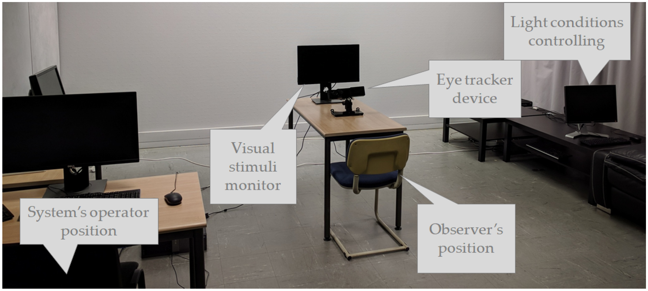
3.3.1. Eye-Tracking Apparatus

A specific setup was designed to capture eye-tracking information on video stimuli. It included a rendering monitor, an eye-tracking system, a control operating system, and a controlled laboratory test room. Figure 2 illustrates the experimental setup used during the collection of gaze information. We can observe the arrangement of all the systems described below.

To run the experiment and collect gaze information, we used the EyeLink^® 1000 Plus eye-tracking system (https://www.sr-research.com/eyelink-1000-plus/), in the head free-to-move remote mode, taking advantage of its embedded 25 mm camera lens. The eye tracker principle is to detect and record the IR illuminator reflection rays on the observer’s pupil [65]. This system enables the collection of highly precise gaze data at a temporal frequency of 1000 Hz and a spatial accuracy between the visual angle range of 0.25 and 0.50 degree, according to the manufacturer. The eye tracker’s camera was configured for each subject, without affecting the corresponding distance between them. This configuration guarantees to achieve an optimal detection of the observer’s eyes and head sticker.

The experimental monitor which displayed stimuli was a 23.8-inch (52.70 × 29.65 cm) DELL P2417H computer monitor display (https://www.dell.com/cd/business/p/dell-p2417h-monitor/pd) with full HD resolution (1920 × 1080) at 60 Hz and with a response time of 6 ms. As suggested by both the International Telecommunication Union (ITU)-Broadcasting Service (television) (BT).710 [67] and manufacturer, observers sat in distances of about 3 H (1 m ± 10 cm) from the monitor, where H corresponds to the stimuli display height so that observers had an assumed spatial visual angle acuity of one degree. Moreover, the eye tracker camera was placed 43 cm away from the experimental display, and thus about 67 cm from participants. Based on this setting, there were 64 pixels per degree of visual angle in each dimension, and the display resolution was about 30 × 17 visual degrees.

Regarding software, the MPC-HC video player (https://mpc-hc.org/), considered as one of the most lightweight open-source video players, rendered the experimental video stimuli. Also, we took advantage of the Eyelink toolbox [68] as it is part of the third version of Psychophysics Toolbox Psychtoolbox-3 (PTB-3) (http://psychtoolbox.org/) and added in-house communication processes (LS2N, University of Nantes) for sync between control and display systems. The control system consists of an additional computer, used by the experimenter to configure and control the eye-tracking system with an Ethernet connection.

Eventually, eye-tracking tests were performed in a room with controlled constant light conditions. The performed calibration set the constant ambient light conditions at approximately 36.5 cd/${\mathrm{m}}^2$, i.e., 15% of the maximum stimuli monitor brightness—249 cm/${\mathrm{m}}^2$—as recommended by the ITU-BT.500 [69], with the i1 Display Pro X-Rite^® system.

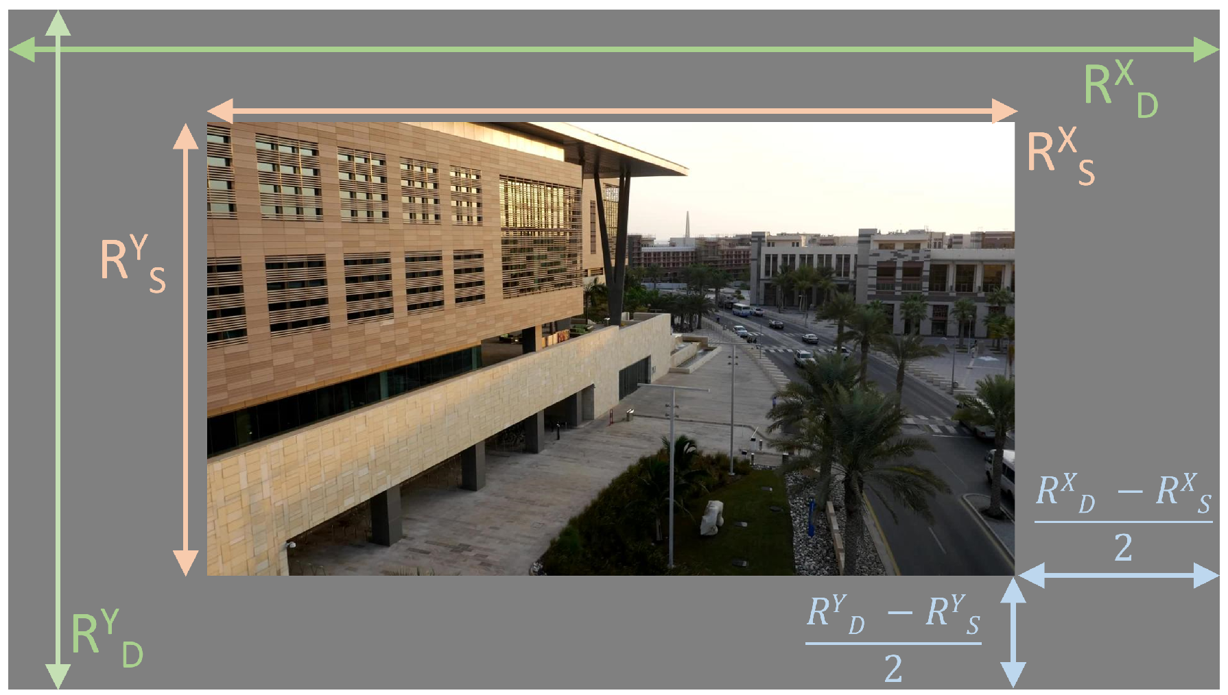
3.3.2. Stimuli Presentation

The random presentation of stimuli in their native resolution centered on the screen prevents ordering, resizing, and locating biases. Knowing that the monitor resolution is higher than that of selected sequences, video stimuli were padded with mid-grey. Additionally, to avoid possible biases in gaze allocation, a 2-second sequence of mid-gray frames was presented before playing a test sequence. Please note that the amount of original information contained in a degree of visual angle was not the same for VIRAT sequences than for other database content, as specified in Table 1.

Before starting the experiment, a training session was organized to get the subject familiar with the experiment design. It included a calibration procedure and its validation followed by the visualization of one video. This UAV video was the sequence car4 from the DTB70 dataset. To avoid any memory bias, this sequence was not included in test stimuli. Once subjects completed the training session, they could ask questions to experimenters before taking part into test sessions.

Regarding test sessions, they started with calibration and its validation. Then followed the visualization of nine videos during which subjects did or did not perform a task. To ensure the optimal quality of the collected gaze data, each participant took part in five test sessions. Splitting the experiment into sessions decreased the tiredness and lack of attention in observers. Also, this design enabled frequent calibration so that recordings did not suffer from the decrease of accuracy in gaze recordings with time [65].

With regards to calibration, the eye-tracking system was calibrated for each participant, following a typical 13 fixed-point detection procedure [65]. Actually, experimenters started tests with a nine-point strategy for calibration (subject 1 to 17 in free viewing (FV)) but realized that using a 13-point calibration produced more accurate gaze collection. The calibration reached validation when the overall deviation of both eye positions was approximately below the fovea vision accuracy (e.g., a degree of visual angle [65,70]). The calibration procedure was repeated until validation.

The participation of an observer in the experiment lasted about 50 min. It included test explanations, forms signing, and taking part in the training and the five test sessions. This duration was acceptable regarding the number of sessions and the fatigue in subjects.

3.3.3. Visual Tasks to Perform

EyeTrackUAV2 aimed to investigate two visual tasks. Indeed, we wanted to be able to witness visual attention processes triggered by top-down (or goal-directed) and bottom-up (or stimulus-driven) attention. Accordingly, we defined two visual tasks participants had to perform: the first condition was an FV task while the second relates to a surveillance viewing task (Task). The former task is rather common in eye-tracking tests [32,37,43,45,50,71]. Observers were simply asked to observe visual video stimuli without performing any task. For the surveillance-viewing task, participants were required to watch video stimuli and to push a specific button on a keyboard each time they observe a new—meaning not presented before—moving object (e.g., people, vehicle, bike, etc.) in the video. The purpose of this task was to simulate one of the basic surveillance procedures in which targets could be located anywhere when the visual search process was performed [72]. After reviewing typical surveillance systems’ abilities [73], we decided to define our task as object detection. The defined object detection task was compelling in that it encompassed target-specific training (repeated discrimination of targets and non-targets) and visual search scanning (targets potentially located anywhere) [72]. The surveillance-viewing task is especially interesting for a military context, in which operators have to detect anomaly in drone videos.

3.3.4. Population

Overall, 30 observers participated in each phase of the test. Tested population samples were different for these two viewing conditions. They were carefully selected to be as diverse as possible. For instance, they include people from more than 12 different countries, namely Algeria (3%), Brazil, Burundi, China, Colombia (10%), France (67%), Gabon, Guinea, South Arabia, Spain, Tunisia, and Ukraine. Additionally, we achieved gender and almost eye-dominance balance in both phases tests.

Table 4. Population characteristics.

Sample Statistics	FV	Task	Total
Participants	30	30	60
Female	16	16	32
Male	14	14	28
Average age	31.7	27.9	29.8
Std age	11.0	8.5	10.0
Min age	20	19	19
Max age	59	55	59
Left dominant eye	19	9	28
Right dominant eye	11	21	32
Participants with glasses	0	4	4

presents the detailed population characteristics for both tasks.

Each observer had been tested for visual acuity and color vision with Ishihara and Snellen tests [74,75]. Any failure of these tests motivated the dismissal of the person from the experiment. Before running the test, the experimenter provided subjects with written consent and information forms, together with oral instructions. This process made sure of the consent of participants and their understanding of the experiment process. It also ensured anonymous data collection.

3.4. Post-Processing of Eye-Tracking Data

First, we transformed collected raw signals into the pixel coordinate system of the original sequence. This conversion led to what we refer to as binocular gaze data. Let us be precise that the origin of coordinates was the top-left corner. Then, any gaze coordinates out of range were evicted, as they did not represent visual attention on stimuli. Once transformed and filtered, we extracted fixation and saccade information and created gaze density maps from gaze data. The remainder of this section describes all post-processing functions.

3.4.1. Raw Data

At first, coordinates of the collected binocular gaze data were transformed into the pixel coordinate system of the visual stimulus. Additionally, we addressed the original resolution of sequences. Coordinates outside the boundaries of the original resolution of the stimulus were filtered out as they were not located in the video stimuli display area. The following formula presents how the collected coordinates are transformed for both eyes:

$$\left\{\begin{array}{cc}{x}_S\hfill & =\lfloor x_D-\frac{R_D^X-R_S^X}{2}\rfloor \hfill \\ y_S\hfill & =\lfloor y_D-\frac{R_D^Y-R_S^Y}{2}\rfloor \hfill \end{array}\right.$$

(1)

where, $(x_S,y_S)$ and $(x_D,y_D)$ are the spatial coordinates on the stimulus and on the display, respectively. The operator $\lfloor .\rfloor$ allowed us to keep the coordinates if the coordinates were within the frame of the stimulus. Otherwise, the coordinate was discarded. $(R_S^X,R_S^Y)$ and $(R_D^X,R_D^Y)$ represent the stimulus resolution and the display resolution, respectively. For more clarity, Figure 3 displays the terms of the equation. Once this remapping had been done for both eyes, the spatial binocular coordinates were simply given by the average of the spatial coordinates of left and right eyes.

During the surveillance-viewing task, subjects pushed a button when detecting an object (never seen before) in the content. Triggering this button action was included in raw data. Consequently, we denotde in raw data a button activation (respectively no detection reaction) with the Boolean value 1 (respectively 0). Besides, for convenience, we extracted the positions of the observer’s dominant eyes and included them in raw gaze data.

3.4.2. Fixation and Saccade Event Detection

To retrieve fixations from eye positions, we used the dispersion-threshold identification (I-DT) [76] from the EyeMMV and LandRate toolboxes [77,78]. This algorithm performed “two-step” spatial and temporal thresholds. As exposed in [78,79], thanks to the very high precision of our eye-tracking equipment, we could combine the two-step spatial thresholds into one operation, as both thresholds had the same value. Ultimately, in our context, this algorithm conceptually implemented a spatial noise removal filter and a temporal threshold indicating the minimum fixation duration. We have selected the minimum threshold values from the state of the art to ensure the performance of the fixation detection algorithm. Accordingly, spatial and temporal thresholds were selected to be equal to $0.7$ degree of visual angle and 80 ms [80], respectively. Finally, saccade events were calculated based on the computed fixations considering that a saccade corresponds to eye movements between two successive fixation points. When considering raw data of the dominant eye, I-DT exhibited a total number of fixations of 1,239,157 in FV and 1,269,433 in Task.

3.4.3. Human Saliency Maps

Saliency maps are a 2D topographic representation indicating the ability of an area to attract observers’ attention. It is common to represent the salience of an image thanks to either its saliency map or by its colored representation, called heatmap. Human saliency maps are usually computed by convolving the fixation map, gathering observers’ fixations, with a Gaussian kernel representing the foveal part of our retina. More details can be found in [71]. In our context, we did not compute convolved fixation maps. We took benefit from the high frequency of acquisition of the eye-tracker system to compute human saliency maps directly from raw gaze data (in pixel coordinates). For the sake of clarity, we from now will refer to the generated saliency maps as gaze density maps.

To represent salient regions of each frame, we followed the method described in [77]. We derived parameters from the experimental setup (e.g., a grid size of a pixel, a standard deviation of 0.5 degree of angle i.e., $\sigma$ = 32 pixels, and a kernel size of 6$\sigma$). For visualization purposes, gaze density maps were normalized between 0 and 255. Figure 4 presents gaze density maps obtained for both attention conditions in frame 100 of seven sequences. We selected frame 100 to get free from the initial center-bias in video exploration occurring during the first seconds. These examples illustrate the sparsity of salience in videos in free viewing, while task-based attention usually presents more salient points, more dispersed in the content than FV, depending on the task and attention-grabbing objects.

3.5. EyeTrackUAV2 in Brief

We have created a dataset containing binocular gaze information collected during two viewing conditions (free viewing and task) over 43 UAV videos (30 fps, 1280 × 720 and 720 × 480—42,241 frames, 1408 s) observed by 30 participants per condition, leading to 1,239,157 fixations in free-viewing and 1,269,433 in task-viewing for dominant eyes positions. Notably, selected UAV videos show diversity in rendered environments, movement and size of objects, aircraft flight heights and angles to the ground, duration, size, and quality. This dataset overcomes the limitations of EyeTrackUAV1 in that it enables investigations of salience in more test sequences, on larger population samples, and for both free-viewing and task-based attention. Additionally, and even though they are still too few, three IR videos are part of visual stimuli.

Fixations, saccades, and gaze density maps were computed—for both eyes in additive and averaged fashions (see Binocular and BothEyes scenarios described later) and for the dominant eye—and are publicly available with original content and raw data on our FTP ftp://[email protected]/EyeTrackUAV2/. The code in MATLAB to generate all ground truth information is also made available.

4. Analyses

In this section, we characterize the proposed EyeTrackUAV2 database. On one hand, we compare salience between six ground truth generation scenarios. This study can be beneficial to the community to know what is the potential error made when selecting a specific ground truth scenario over another. On the other hand, UAV videos induce new visual experiences. Consequently, observers exhibit different behaviors towards this type of stimuli. Therefore, we investigate whether the center bias, one of the main viewing tendencies [28], still applies to EyeTrackUAV2 content.

4.1. Six Different Ground Truths

The first question we address concerns the method used to determine the ground truth. In a number of papers, researchers use the ocular dominance theory in order to generate the ground truth. This theory relies on the fact that the human visual system favors the input of one eye over the other should binocular images be too disparate on the retinas. However, the cyclopean theory gains more and more momentum [81,82]. It alleges that vision processes approximate a central point between two eyes, from which an object is perceived. Furthermore, lately, manufacturers achieved major improvements in eye-tracking systems. They are now able to record and calibrate the positions of both eyes separately. This allows for exploring what best practices to create salient ground truth are [81,82,83].

When examining the mean of absolute error between eye positions of all scenarios, we have found a maximum value of about 0.6 degrees of visual angle. That value is rather small compared to the Gaussian kernel convolved on eye positions. Thus, we question whether selecting a ground truth scenario over another makes a significant difference for saliency studies. Consequently, we compared gaze density maps generated for the six scenarios defined below.

We proposed to evaluate the potential errors made when different methods for creating the ground truth are used. Note that the true position of the user gaze is not available. Accordingly, we need to run a cross-comparison between several well-selected and representative ground truths. Scenarios highly similar to all others are the ones that will make fewer errors. In such a context, the more scenarios are included, the more complete and reliable the study is.

We tested six methods, namely left (L), right (R), binocular (B), dominant (D), non-dominant (nD), and both eyes (BE). B corresponds to the average position between the left and right eyes and can be called version signal (see Equation (2)). BE includes the positions of both L and R eyes, and hence comprises twice as much information as other scenarios (see Equation (3)). nD has been added to estimate the gain made when using dominant eye information. The two visual attention conditions FV and Task were examined in this study. Illustrations of scenarios gaze density maps and fixations as well as methods comparisons are presented in Figure 5. Below is presented the quantitative evaluation.

$$\left\{\begin{array}{cc}{x}_B\hfill & =\lfloor \frac{x_L+x_R}{2}\rfloor \hfill \\ y_B\hfill & =\lfloor \frac{y_L+y_R}{2}\rfloor \hfill \end{array}\right.$$

(2)

$$\left\{\begin{array}{cc}{x}_{BE}\hfill & =x_L\cup x_R\hfill \\ y_{BE}\hfill & =y_L\cup y_R\hfill \end{array}\right.$$

(3)

We ran a cross-comparison on six well-used saliency metrics: correlation coefficient (CC) ($\in \left[-1,1\right]$), similarity (SIM) ($\in \left[0,1\right]$) the intersection between histograms of saliency, area under the curve (AUC) Judd and Borji ($\in \left[0,1\right]$), normalized scanpath saliency (NSS) ($\in \left]-\infty ,+\infty \right[$), and information gain (IG) ($\in \left[0,+\infty \right[$), which measures on average the gain in information contained in the saliency map compared to a prior baseline ($\in \left[0,+\infty \right[$). We did not report Kullback–Leibler divergence (KL) ($\in \left[0,+\infty \right[$) as we favored symmetric metrics. Moreover, even though symmetric in absolute value, IG provides different scores depending on fixations under consideration. We thus compared scenarios for fixations of both methods, which leads to two IG measures. More details on metrics and metrics behaviors are given in [36,71,84].

Table 5. Correlation coefficient (CC), similarity (SIM), and information gain (IG) results for scenarios cross-comparison. Red indicates the best scores and blue the least.

		FV				Task
		CC ↑	SIM ↑	IG ↓		CC ↑	SIM ↑	IG ↓
SM1	SM2			SM1-Fix1-SM2	SM2-Fix2-SM1			SM1-Fix1-SM2	SM2-Fix2-SM1
Binocular	Dominant	0.94	0.83	0.377	0.300	0.952	0.850	0.276	0.148
Binocular	EyeNonDom	0.95	0.84	0.370	0.301	0.952	0.849	0.283	0.163
Binocular	Left	0.94	0.83	0.371	0.301	0.948	0.843	0.264	0.192
Binocular	Right	0.94	0.83	0.390	0.324	0.944	0.838	0.304	0.152
Binocular	BothEyes	0.98	0.90	0.246	0.139	0.983	0.916	0.177	0.012
Dominant	BothEyes	0.96	0.87	0.158	0.374	0.967	0.873	0.143	0.248
EyeNonDom	BothEyes	0.97	0.87	0.167	0.394	0.966	0.872	0.144	0.228
Left	BothEyes	0.96	0.86	0.166	0.387	0.960	0.861	0.174	0.232
Right	BothEyes	0.96	0.86	0.181	0.416	0.960	0.862	0.147	0.279
Dominant	EyeNonDom	0.87	0.74	1.115	1.069	0.873	0.747	0.743	0.781
Dominant	Left	0.95	0.88	0.341	0.339	0.903	0.792	0.520	0.582
Dominant	Right	0.91	0.79	0.810	0.757	0.957	0.884	0.256	0.233
EyeNonDom	Right	0.96	0.88	0.346	0.342	0.902	0.793	0.587	0.519
Left	EyeNonDom	0.91	0.79	0.792	0.754	0.957	0.884	0.256	0.231
Left	Right	0.85	0.72	1.176	1.121	0.850	0.725	0.877	0.782
Mean		0.937	0.832	0.467	0.488	0.938	0.839	0.343	0.319
Std		0.037	0.052	0.340	0.295	0.038	0.053	0.230	0.234

presents the results of measures when comparing gaze density maps of two scenarios.

Here are some insights extracted from the results:

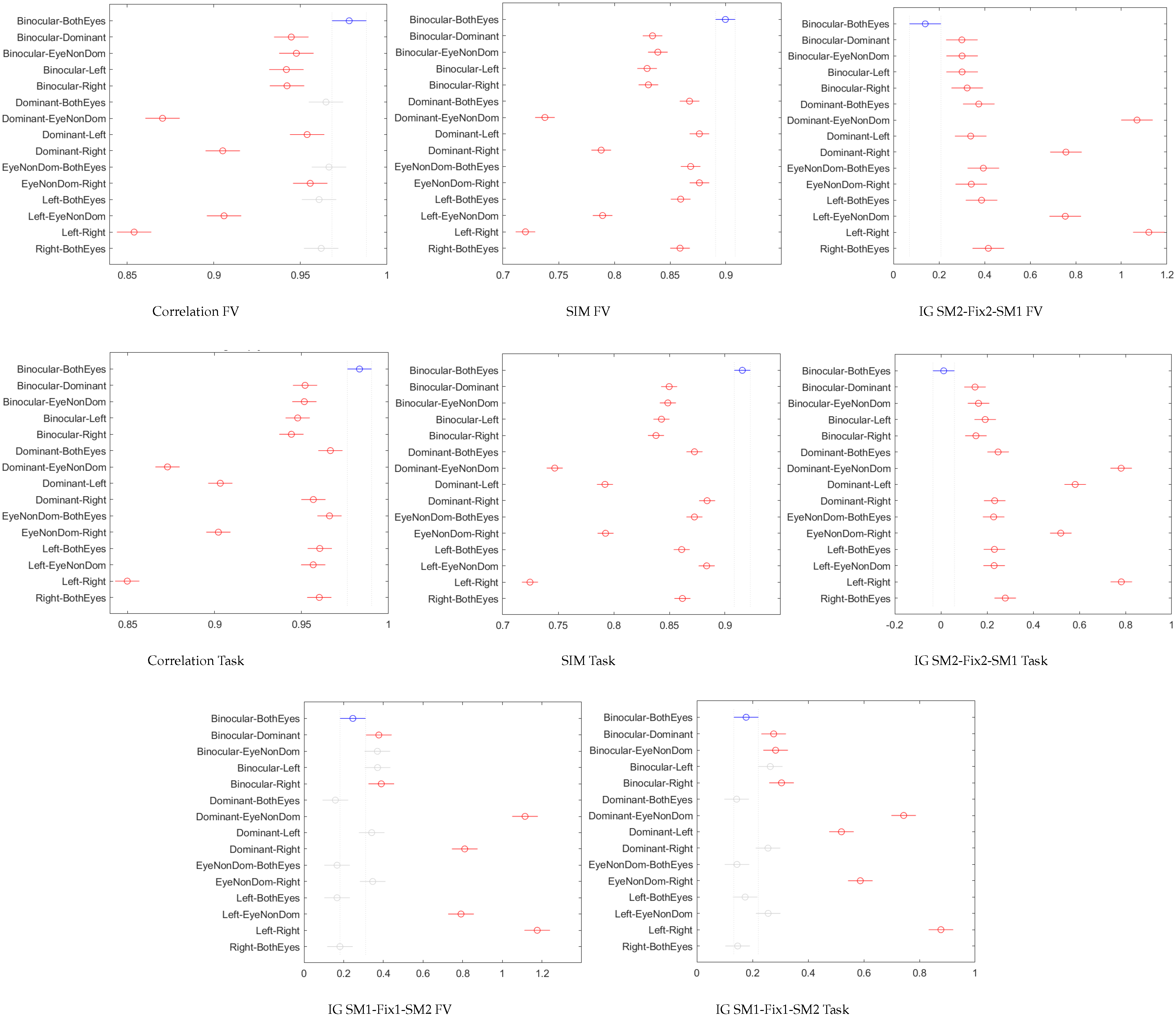
• There was a high similarity between scenario gaze density maps. As expected, scores were pretty high (respectively low for IG), which indicates the high similarity between scenarios.
• All metrics showed the best results for comparisons including Binocular and BothEyes scenarios, the highest being the Binocular-BothEyes comparison.
• Left–Right and Dominant–NonDominant comparisons achieved worst results.
• It was possible to know the population main dominant eye through scenario comparisons (not including two eyes information). When describing the population, we saw that a majority of left-dominant-eye subjects participated in the FV test, while the reverse happened for the Task experiment. This fact is noticeable in metric scores.

To verify whether scenarios present statistically significant differences, we have conducted an analysis of variance (ANOVA) on the scores obtained by the metrics. ANOVA results are presented in

Table 6. ANOVA analysis.

		FV		Task
		F-Value	p-Value	F-Value	p-Value
$p<0.05$	CC	F(14,630) = 77.72	$5\times {10}^{-127}$	F(14,630) = 172.55	$9\times {10}^{-205}$
	SIM	F(14,630) = 200.07	$5\times {10}^{-221}$	F(14,630) = 309.43	$2\times {10}^{-271}$
	IG	F(14,630) = 158.96	$5\times {10}^{-196}$	F(14,630) = 156.16	$4\times {10}^{-194}$
$p>0.05$	AUCJ	F(14,630) = 0.36	0.9857	F(14,630) = 0.4	0.9742
	AUCB	F(14,630) = 0.22	0.9989	F(14,630) = 0.05	1
	NSS	F(14,630) = 0.95	0.5036	F(14,630) = 0.92	0.5344

. All metrics showed statistically different results ($p<0.05$) except for AUC Borji, AUC Judd, and NSS. It shows that, with regard to these three metrics, using a scenario over another makes no significant difference. This also explains why we did not report AUC and NNS results in Table 5. We further explore the other metrics, namely CC, SIM, and IG, through the Tukey’s multiple comparison post-hoc test [85] ($\alpha =0.05$).

Results are presented in Figure 6. On the charts, we can see where stands group means and comparison intervals for each scenario over the entire dataset. Scenarios having non-overlapping intervals are statistically different.

In details, our results show three statistically distinct categories for all metrics.

• The first category showed the best similarities (i.e., highest for CC and SIM, and lowest for IGs) between scenarios, include all comparisons involving B and BE scenarios. There are also comparisons between single eye signals being the most and the least representative of the population’s eyedness (e.g., D vs L and nD vs R for FV, D vs R and nD vs L for Task).
• The second category included the comparison of single eye signals that do not represent the “same” population’s eyedness (i.e., D vs R and nD vs L for FV, D vs L and nD vs R for Task)
• Lastly, the third category presented the least similar scenario comparisons, in terms of the four evaluated metrics. Those comparisons are the single eye signals that come from different eyes (i.e., L vs R and D vs nD). Let us note that metrics gave reasonably good similarity scores, even for these two scenarios.

Also, there are some behaviors not common to all metrics that are worth mentioning. On one hand, for SIM and IG SM2–Fix2–SM1 in FV and Task, as well as for CC Task, scenario B vs. BE statistically achieved the best similarity scores. This strengthens even more the interest to use B or BE scenarios. On the other hand, for all metrics under the Task condition, and for SIM FV, the scenario L vs R was statistically different from D vs. nD. It also presented the least CC and SIM and the highest IG scores. This shows that under certain conditions, especially for Task attention in our context, D and nD scenarios may be favored over L and R signals.

Overall, over six metrics, three did not find significant differences between the scenarios’ gaze density maps. The four others did, and indicated that using both eye information can be encouraged. Then, if not possible, eye-dominance-based signals may be favored over left and right eye scenarios, in particular under task-based attention. We stress out that overall, the difference between scenarios is rather small, as three metrics could not differentiate them.

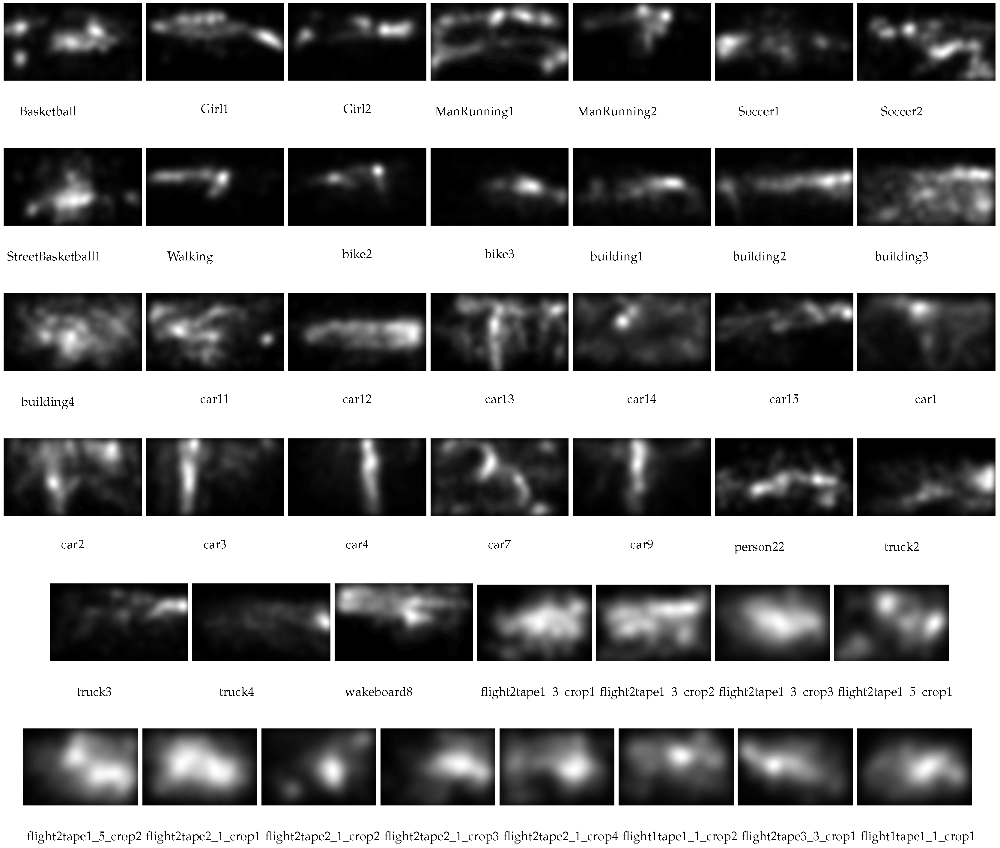
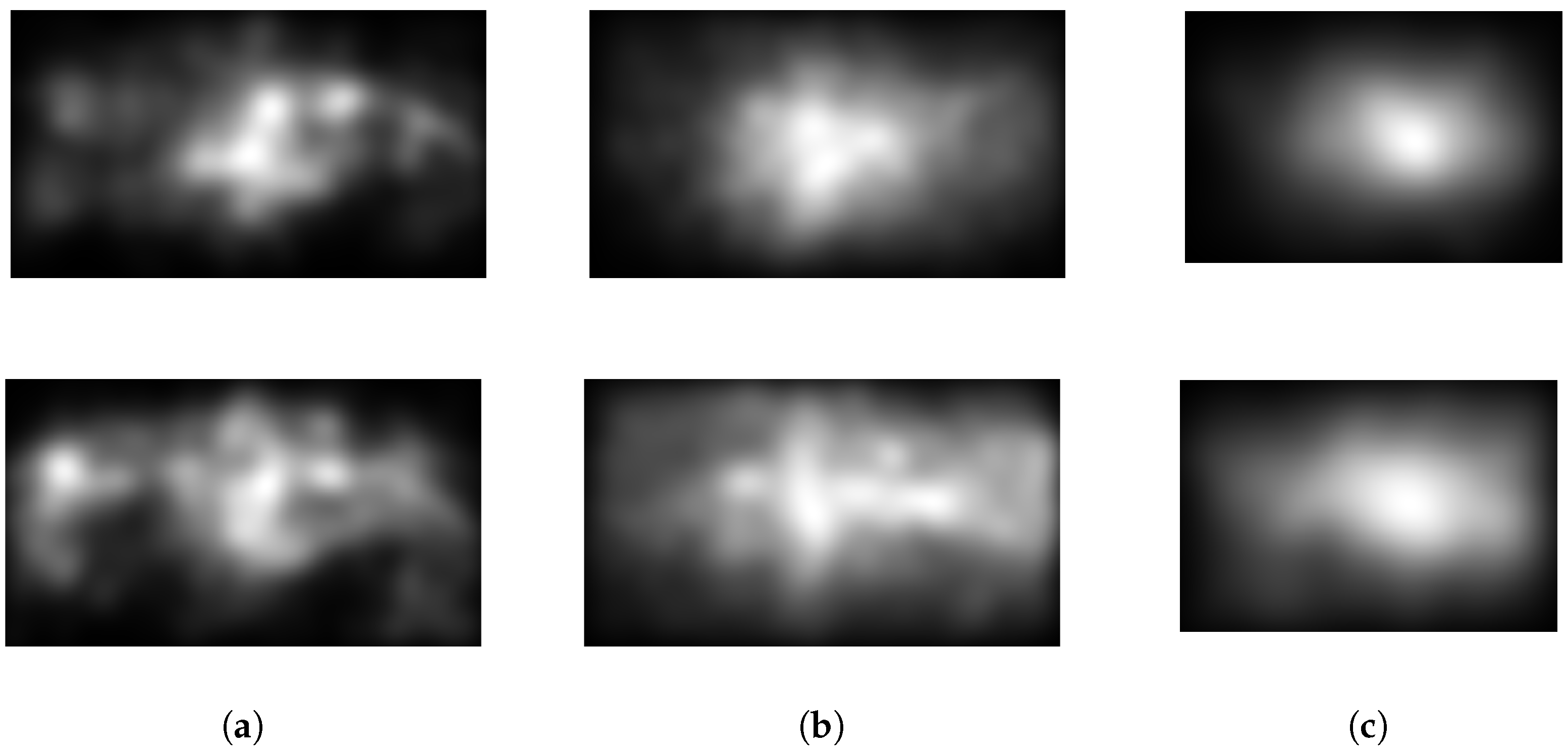
4.2. Biases in UAV Videos

The importance of the center bias in visual saliency for conventional imaging has been shown in Section 2. We wondered whether the center bias is systematically present in UAV content. This section aims to shed light on this question, qualitatively and quantitatively.

4.2.1. Qualitative Evaluation of Biases in UAV Videos

We evaluated the viewing tendencies of observers thanks to the average gaze density map, computed over the entire sequence. It was representative of the average position of gaze throughout the video. It was used to observe potential overall biases, as it could be the case with the center bias. Figure 7 and Figure 8 show the average gaze density map for all sequences of EyeTrackUAV2 dataset, generated from D scenario, for both free-viewing and task-viewing conditions. Several observations can be made.

Content-dependent center bias. We verify here the content-dependence of the center bias in UAV videos. For both attention conditions, the scene environment and movements exacerbates or not UAV biases. For instance, in sequences car 2–9 (fourth row), the aircraft is following cars on a road. Associated average gaze density maps display the shape of the road and its direction, i.e., vertical route for all and roundabout for car7. Car 14 (third row), a semantically similar content except that it displays only one object on the road with a constant reframing (camera movement) which keeps the car at the same location, presents an average gaze density map centered on the tracked object.

Original database-specific center bias. We can observe that a center bias was present in VIRAT sequences, while videos from other datasets, namely UAV123 and DTB70, did not present this bias systematically. The original resolution of content and the experimental setup are possibly the sources of this result. Indeed, the proportion of content seen at once was not the same for all sequences: 1.19% of a VIRAT content was seen per degree of visual angle, whereas it was 0.44% for the two other original databases. VIRAT gaze density maps were thus smoother, which resulted in higher chances to present a center bias. To verify this assumption based on qualitative assessment, we computed the overall gaze density maps for sequences coming from each original dataset, namely DTB70, UAV123, and VIRAT. These maps are shown in Figure 9. VIRAT gaze density maps are much more concentrated and centered. This corroborates that biases can be original-database-specific.

Task-related gaze density maps seemed more spread out. Task-based gaze density maps covered more content when compared to free-viewing condition for most sequences (e.g., in about 58% of videos such as basketball, car11, car2, and wakeboard). This behavior is also illustrated in Figure 9. We correlate this response with the object detection task. Visual search scanning implies an extensive exploration of the content. However, 21% of the remaining sequences (i.e., soccer1, bike2–3, building 1–2, car1 and 15, and truck3–4) show less discrepancies in the task-viewing condition than in free-viewing condition. We do not find correlation between such behavior and sequences characteristics given in Table 3. This leaves room for further exploration of differences between task-based and free viewing attention.

Overall, there was no generalization of center bias for UAV content. As stated earlier, we do not observe a systematic center bias, except for VIRAT sequences. This is especially true for task-related viewing. However, we observe specific patterns. Indeed, vertical and horizontal potato-shaped salient areas are quite present in average gaze density maps of EyeTrackUAV2. Such patterns are also visible in UAV2 and DTB70 overall gaze density maps, especially in task-viewing condition. This indicates future axes of developments for UAV saliency-based applications. For instance, instead of using a center bias, one may introduce priors as a set of prevalent saliency area shapes with different directions and sizes [86].

4.2.2. Quantitative Evaluation of the Central Bias in UAV Videos

To go further into content-dependencies, we investigated quantitatively the similarity of dominant-eye-generated gaze density maps with a pre-defined center bias. Figure 10 presents the center bias baseline created in this purpose as suggested in [35,36].

We performed the evaluation based on four well-used saliency metrics: CC, SIM, KL, and IG. Results are presented in

Table 7. Comparison of gaze density maps with the center bias presented in Figure 10. Are displayed in red the numbers over (or under for Kullback–Leibler divergence (KL) and IG) measures average, indicated in the last row.

	FV				Task
	CC ↑	SIM ↑	KL ↓	IG ↓	CC↑	SIM ↑	KL ↓	IG ↓
VIRAT_09152008flight2tape1_3_crop1	0.50	0.48	7.17	1.53	0.46	0.48	6.85	1.62
VIRAT_09152008flight2tape1_3_crop2	0.49	0.52	5.59	1.50	0.36	0.48	6.42	1.75
VIRAT_09152008flight2tape1_3_crop3	0.46	0.43	8.46	1.91	0.37	0.43	7.98	1.99
VIRAT_09152008flight2tape1_5_crop1	0.27	0.38	9.77	2.29	0.18	0.36	10.14	2.49
VIRAT_09152008flight2tape1_5_crop2	0.42	0.44	8.05	1.90	0.30	0.45	7.41	1.87
VIRAT_09152008flight2tape2_1_crop1	0.41	0.39	9.34	2.05	0.38	0.42	8.55	1.97
VIRAT_09152008flight2tape2_1_crop2	0.40	0.35	10.90	2.50	0.32	0.42	8.01	2.01
VIRAT_09152008flight2tape2_1_crop3	0.42	0.40	9.46	2.11	0.28	0.39	9.30	2.24
VIRAT_09152008flight2tape2_1_crop4	0.36	0.36	10.35	2.34	0.28	0.38	9.79	2.30
VIRAT_09152008flight2tape3_3_crop1	0.42	0.43	8.16	1.96	0.35	0.43	7.84	2.03
VIRAT_09162008flight1tape1_1_crop1	0.47	0.45	7.76	1.80	0.37	0.42	8.40	2.00
VIRAT_09162008flight1tape1_1_crop2	0.40	0.40	9.14	2.14	0.27	0.40	8.91	2.22
UAV123_bike2	0.39	0.34	11.51	2.43	0.34	0.29	13.21	2.82
UAV123_bike3	0.39	0.34	11.71	2.37	0.29	0.26	14.34	2.96
UAV123_building1	0.40	0.37	10.64	2.18	0.32	0.31	12.74	2.69
UAV123_building2	0.30	0.33	11.89	2.43	0.18	0.27	13.87	3.06
UAV123_building3	0.27	0.34	11.50	2.42	0.17	0.32	11.82	2.56
UAV123_building4	0.39	0.36	10.82	2.20	0.35	0.39	9.72	2.10
UAV123_car11	0.37	0.32	12.37	2.58	0.21	0.30	12.68	2.67
UAV123_car12	0.21	0.28	13.35	2.80	0.26	0.29	13.12	2.69
UAV123_car13	0.30	0.34	11.48	2.39	0.20	0.33	11.50	2.44
UAV123_car14	0.20	0.25	14.47	3.16	0.12	0.31	12.28	2.71
UAV123_car15	0.31	0.34	11.52	2.47	0.10	0.30	12.70	2.81
UAV123_car1	0.21	0.26	14.33	3.10	0.13	0.30	12.61	2.77
UAV123_car2	0.22	0.27	13.91	3.02	0.13	0.30	12.68	2.80
UAV123_car3	0.16	0.24	14.77	3.19	0.14	0.28	13.39	2.93
UAV123_car4	0.22	0.20	16.27	3.55	0.20	0.24	14.76	3.23
UAV123_car7	0.22	0.23	15.11	3.16	0.11	0.28	13.13	2.92
UAV123_car9	0.26	0.23	15.41	3.27	0.21	0.28	13.69	2.86
UAV123_person22	0.35	0.31	12.44	2.60	0.27	0.31	12.45	2.68
UAV123_truck2	0.27	0.32	12.29	2.56	0.09	0.27	13.66	3.01
UAV123_truck3	0.27	0.35	11.14	2.34	0.12	0.31	12.23	2.73
UAV123_truck4	0.29	0.36	10.71	2.34	0.16	0.29	13.18	3.03
UAV123_wakeboard8	0.23	0.21	15.91	3.45	0.11	0.24	14.93	3.29
DTB70_Basketball	0.38	0.27	14.13	2.89	0.30	0.31	12.30	2.59
DTB70_Girl1	0.16	0.28	13.47	2.90	0.15	0.25	14.54	3.18
DTB70_Girl2	0.20	0.20	16.04	3.60	0.19	0.23	15.04	3.34
DTB70_ManRunning1	0.02	0.16	17.45	4.09	0.00	0.20	16.11	3.73
DTB70_ManRunning2	0.12	0.13	18.40	4.31	0.10	0.15	17.99	4.24
DTB70_Soccer1	0.21	0.26	14.23	3.04	0.17	0.26	14.03	3.18
DTB70_Soccer2	0.21	0.22	15.56	3.33	0.22	0.32	11.86	2.69
DTB70_StreetBasketball1	0.33	0.26	14.29	2.94	0.28	0.26	14.29	3.00
DTB70_Walking	0.29	0.20	16.14	3.51	0.27	0.22	15.81	3.51
mean	0.31	0.32	12.27	2.67	0.23	0.32	12.01	2.69

. They support the observations we made in the previous section. Overall scores do not reveal a high similarity with the center prior (e.g., maximum CC and SIM of about 0.5, high KL and IG). On the other hand, we observe content-specific center prior in UAV123 and DTB70. For instance, videos more prone to center bias includes sequences extracted from VIRAT and building1,3,4, and car13. On the contrary, sequences Girl1-2, ManRunning1-2, Walking, car4, and wakeboard8 are not likely to present center bias. This confirms there is no generalization of center bias for UAV content. Regarding differences between free-viewing and task-viewing conditions, results are inconclusive as no systematic behavior is clearly visible from this analysis.

5. Conclusions

UAV imaging modifies the perceptual clues of typical scenes due to its bird point of view, the presence of camera movements and the high distance and angle to the scene. For instance, low-level visual features, and size of objects change and depth information is flattened or disappears (e.g., presence of sky). To understand observers’ behaviors toward these new features, especially in terms of visual attention and deployment, there is a need for large-scale eye-tracking databases for saliency in UAV videos. This dataset is also a key factor in the field of computational models of visual attention, in which large scale datasets are required to train the latest generation of deep-based models.

This need is even stronger with the fast expansion of applications related to UAV, for leisure and professional civilian activities and a wide range of military services. Combining UAV imagery with one of the most dynamic research fields in vision, namely salience, is highly promising, especially for videos that are gaining more and more attention these last years.

This work addresses the need for such a dedicated dataset. An experimental process has been designed in order to build a new dataset, EyeTrackUAV2. Gaze data were collected during the observation of UAV videos under controlled laboratory conditions for both free viewing and object-detection surveillance task conditions. Gaze positions have been collected on 30 participants for each attention condition, on 43 UAV videos in 30 fps, 1280 × 720 or 720 × 480, consisting of 42,241 frames and 1408 s. Overall, 1,239,157 fixations in free-viewing and 1,269,433 in task-viewing were extracted from the dominant eye positions. Test stimuli were carefully selected from three original datasets, i.e., UAV123, VIRAT, and DTB70, to be representative as much as possible of the UAV ecosystem. Accordingly, they present variations in terms of environments, camera movement, size of objects, aircraft flight heights and angles to the ground, video duration, resolution, and quality. Also, three sequences were recorded in infra-red.

The collected gaze data were analyzed and transformed into fixation and saccade eye movements using an I-DT-based identification algorithm. Moreover, the eye-tracking system high frequency of acquisition enabled the production of gaze density maps for each experimental frame of the examined video stimuli directly from raw data. The dataset is publicly available and includes, for instance, raw binocular eye positions, fixation, and gaze density maps generated from the dominant eye and both eyes information.

We further characterized the dataset considering two different aspects. On one hand, six scenarios, namely binocular, both eyes, dominant eye, non-dominant eye, left, and right can be envisioned to generate gaze density maps. We wondered whether a scenario should be favored over another or not. Comparisons of scenarios have been conducted on six typical saliency metrics for gaze density maps. Overall, all scenarios are pretty similar: over the six evaluated metrics, three could not make a distinction between scenarios. The three last metrics present mild but statistically significant differences. Accordingly, the information of both eyes may be favored to study saliency. If not possible, choosing information from the dominant eye is encouraged. This advice is not a strict recommendation. On the other hand, we notice that conventional biases in saliency do not necessarily apply to UAV content. Indeed, the center bias is not systematic in UAV sequences. This bias is content-dependent as well as and task-condition-dependent. We observed new prior patterns that must be examined in the future.

In conclusion, the EyeTrackUAV2 dataset enables in-depth studies of visual attention through the exploration of new salience biases and prior patterns. It establishes in addition a solid basis on which dynamic salience for UAV imaging can build upon, in particular for the development of deep-learning saliency models.

References

1. Zhao, Y.; Ma, J.; Li, X.; Zhang, J. Saliency detection and deep learning-based wildfire identification in UAV imagery. Sensors 2018, 18, 712. [Google Scholar] [CrossRef] [Green Version]
2. Van Gemert, J.C.; Verschoor, C.R.; Mettes, P.; Epema, K.; Koh, L.P.; Wich, S. Nature conservation drones for automatic localization and counting of animals. In Workshop at the European Conference on Computer Vision; Springer: Zurich, Switzerland, 2014; pp. 255–270. [Google Scholar]
3. Postema, S. News Drones: An Auxiliary Perspective; Edinburgh Napier University: Scotland, UK, 2015. [Google Scholar]
4. Agbeyangi, A.O.; Odiete, J.O.; Olorunlomerue, A.B. Review on UAVs used for aerial surveillance. J. Multidiscip. Eng. Sci. Technol. 2016, 3, 5713–5719. [Google Scholar]
5. Lee-Morrison, L. State of the Art Report on Drone-Based Warfare; Division of Art History and Visual Studies, Department of Arts and Cultural Sciences, Lund University: Lund, Sweden, 2014. [Google Scholar]
6. Zhou, Y.; Tang, D.; Zhou, H.; Xiang, X.; Hu, T. Vision-based online localization and trajectory smoothing for fixed-wing UAV tracking a moving target. In Proceedings of the IEEE International Conference on Computer Vision Workshops, Seoul, Korea, 27 October–2 November 2019. [Google Scholar]
7. Zhu, P.; Du, D.; Wen, L.; Bian, X.; Ling, H.; Hu, Q.; Peng, T.; Zheng, J.; Wang, X.; Zhang, Y.; et al. VisDrone-VID2019: The vision meets drone object detection in video challenge results. In Proceedings of the IEEE International Conference on Computer Vision Workshops, Seoul, Korea, 27 October–2 November 2019. [Google Scholar]
8. Aguilar, W.G.; Luna, M.A.; Moya, J.F.; Abad, V.; Ruiz, H.; Parra, H.; Angulo, C. Pedestrian detection for UAVs using cascade classifiers and saliency maps. In Proceedings of the International Work-Conference on Artificial Neural Networks, Càdiz, Spain, 14–16 June 2017; pp. 563–574. [Google Scholar]
9. Dang, T.; Khattak, S.; Papachristos, C.; Alexis, K. Anomaly detection and cognizant path planning for surveillance operations using aerial robots. In Proceedings of the 2019 International Conference on Unmanned Aircraft Systems (ICUAS), Atlanta, GA, USA, 11–14 June 2019; pp. 667–673. [Google Scholar]
10. Edney-Browne, A. Vision, visuality, and agency in the US drone program. In Technology and Agency in International Relations; Routledge: Abingdon, UK, 2019; p. 88. [Google Scholar]
11. Krassanakis, V.; Perreira Da Silva, M.; Ricordel, V. Monitoring human visual behavior during the observation of unmanned aerial vehicles (UAVs) videos. Drones 2018, 2, 36. [Google Scholar] [CrossRef] [Green Version]
12. Howard, I.P.; Rogers, B. Depth perception. Stevens Handb. Exp. Psychol. 2002, 6, 77–120. [Google Scholar]
13. Foulsham, T.; Kingstone, A.; Underwood, G. Turning the world around: Patterns in saccade direction vary with picture orientation. Vis. Res. 2008, 48, 1777–1790. [Google Scholar] [CrossRef] [PubMed]
14. Papachristos, C.; Khattak, S.; Mascarich, F.; Dang, T.; Alexis, K. Autonomous aerial robotic exploration of subterranean environments relying on morphology–aware path planning. In Proceedings of the 2019 International Conference on Unmanned Aircraft Systems (ICUAS), Atlanta, GA, USA, 11–14 June 2019; pp. 299–305. [Google Scholar]
15. Itti, L.; Koch, C. Computational modelling of visual attention. Nat. Rev. Neurosci. 2001, 2, 194. [Google Scholar] [CrossRef] [Green Version]
16. Katsuki, F.; Constantinidis, C. Bottom-up and top-down attention: Different processes and overlapping neural systems. Neuroscientist 2014, 20, 509–521. [Google Scholar] [CrossRef]
17. Krasovskaya, S.; MacInnes, W.J. Salience models: A computational cognitive neuroscience review. Vision 2019, 3, 56. [Google Scholar] [CrossRef] [Green Version]
18. Rai, Y.; Le Callet, P.; Cheung, G. Quantifying the relation between perceived interest and visual salience during free viewing using trellis based optimization. In Proceedings of the 2016 IEEE 12th Image, Video, and Multidimensional Signal Processing Workshop (IVMSP), Bordeaux, France, 11–12 July 2016; pp. 1–5. [Google Scholar]
19. Kummerer, M.; Wallis, T.S.; Bethge, M. Saliency benchmarking made easy: Separating models, maps and metrics. In Proceedings of the European Conference on Computer Vision (ECCV), Munich, Germany, 8–14 September 2018; pp. 770–787. [Google Scholar]
20. Riche, N.; Duvinage, M.; Mancas, M.; Gosselin, B.; Dutoit, T. Saliency and human fixations: State-of-the-art and study of comparison metrics. In Proceedings of the IEEE International Conference on Computer Vision, Sydney, Australia, 1–8 December 2013; pp. 1153–1160. [Google Scholar]
21. Guo, C.; Zhang, L. A novel multiresolution spatiotemporal saliency detection model and its applications in image and video compression. IEEE Trans. Image Process. 2009, 19, 185–198. [Google Scholar]
22. Jain, S.D.; Xiong, B.; Grauman, K. Fusionseg: Learning to combine motion and appearance for fully automatic segmentation of generic objects in videos. In Proceedings of the 2017 IEEE Conference on Computer Vision and Pattern Recognition, Honolulu, HI, USA, 21–26 July 2017; pp. 2117–2126. [Google Scholar]
23. Wang, W.; Shen, J.; Shao, L. Video salient object detection via fully convolutional networks. IEEE Trans. Image Process. 2017, 27, 38–49. [Google Scholar] [CrossRef] [Green Version]
24. Li, G.; Xie, Y.; Wei, T.; Wang, K.; Lin, L. Flow guided recurrent neural encoder for video salient object detection. In Proceedings of the IEEE Conference on Computer Vision and Pattern Recognition, Salt Lake City, UT, USA, 18–22 June 2018; pp. 3243–3252. [Google Scholar]
25. Le Meur, O.; Coutrot, A.; Liu, Z.; Rämä, P.; Le Roch, A.; Helo, A. Visual attention saccadic models learn to emulate gaze patterns from childhood to adulthood. IEEE Trans. Image Process. 2017, 26, 4777–4789. [Google Scholar] [CrossRef] [PubMed] [Green Version]
26. Brunye, T.T.; Martis, S.B.; Horner, C.; Kirejczyk, J.A.; Rock, K. Visual salience and biological motion interact to determine camouflaged target detectability. Appl. Ergon. 2018, 73, 1–6. [Google Scholar] [CrossRef] [PubMed]
27. Perrin, A.F.; Zhang, L.; Le Meur, O. How well current saliency prediction models perform on UAVs videos? In Proceedings of the International Conference on Computer Analysis of Images and Patterns, Salerno, Italy, 2–6 Spetember 2019; pp. 311–323. [Google Scholar]
28. Bindemann, M. Scene and screen center bias early eye movements in scene viewing. Vis. Res. 2010, 50, 2577–2587. [Google Scholar] [CrossRef] [Green Version]
29. Tseng, P.H.; Carmi, R.; Cameron, I.G.; Munoz, D.P.; Itti, L. Quantifying center bias of observers in free viewing of dynamic natural scenes. J. Vis. 2009, 9, 4. [Google Scholar] [CrossRef] [PubMed]
30. Van Opstal, A.; Hepp, K.; Suzuki, Y.; Henn, V. Influence of eye position on activity in monkey superior colliculus. J. Neurophysiol. 1995, 74, 1593–1610. [Google Scholar] [CrossRef] [PubMed]
31. Tatler, B.W. The central fixation bias in scene viewing: Selecting an optimal viewing position independently of motor biases and image feature distributions. J. Vis. 2007, 7, 4. [Google Scholar] [CrossRef] [PubMed] [Green Version]
32. Le Meur, O.; Liu, Z. Saccadic model of eye movements for free-viewing condition. Vis. Res. 2015, 116, 152–164. [Google Scholar] [CrossRef]
33. Vigier, T.; Da Silva, M.P.; Le Callet, P. Impact of visual angle on attention deployment and robustness of visual saliency models in videos: From SD to UHD. In Proceedings of the 2016 IEEE International Conference on Image Processing (ICIP), Phoenix, AZ, USA, 25–28 September 2016; pp. 689–693. [Google Scholar]
34. Zhang, K.; Chen, Z. Video saliency prediction based on spatial-temporal two-stream network. IEEE Trans. Circuits Syst. Video Technol. 2018. [Google Scholar] [CrossRef]
35. Le Meur, O.; Le Callet, P.; Barba, D.; Thoreau, D. A coherent computational approach to model bottom-up visual attention. IEEE Trans. Pattern Anal. Mach. Intell. 2006, 28, 802–817. [Google Scholar] [CrossRef] [Green Version]
36. Bylinskii, Z.; Judd, T.; Oliva, A.; Torralba, A.; Durand, F. What do different evaluation metrics tell us about saliency models? IEEE Trans. Pattern Anal. Mach. Intell. 2019, 41, 740–757. [Google Scholar] [CrossRef] [Green Version]
37. Paglin, M.; Rufolo, A.M. Heterogeneous human capital, occupational choice, and male-female earnings differences. J. Labor Econ. 1990, 8, 123–144. [Google Scholar] [CrossRef]
38. Ehinger, K.A.; Hidalgo-Sotelo, B.; Torralba, A.; Oliva, A. Modelling search for people in 900 scenes: A combined source model of eye guidance. Vis. Cogn. 2009, 17, 945–978. [Google Scholar] [CrossRef] [PubMed] [Green Version]
39. Liu, H.; Heynderickx, I. Studying the added value of visual attention in objective image quality metrics based on eye movement data. In Proceedings of the 2009 16th IEEE International Conference on Image Processing (ICIP), Cairo, Egypt, 7–10 November 2009; pp. 3097–3100. [Google Scholar]
40. Judd, T.; Durand, F.; Torralba, A. A Benchmark of Computational Models of Saliency to Predict Human Fixations; Computer Science and Artificial Intelligence Laboratory Technical Report; MIT Library: Cambridge, MA, USA, 2012. [Google Scholar]
41. Ma, K.T.; Sim, T.; Kankanhalli, M. VIP: A unifying framework for computational eye-gaze research. In Proceedings of the International Workshop on Human Behavior Understanding, Barcelona, Spain, 22 October 2013; pp. 209–222. [Google Scholar]
42. Koehler, K.; Guo, F.; Zhang, S.; Eckstein, M.P. What do saliency models predict? J. Vis. 2014, 14, 14. [Google Scholar] [CrossRef] [PubMed]
43. Borji, A.; Itti, L. Cat2000: A large scale fixation dataset for boosting saliency research. arXiv 2015, arXiv:1505.03581. [Google Scholar]
44. Bylinskii, Z.; Isola, P.; Bainbridge, C.; Torralba, A.; Oliva, A. Intrinsic and extrinsic effects on image memorability. Vis. Res. 2015, 116, 165–178. [Google Scholar] [CrossRef] [PubMed]
45. Fan, S.; Shen, Z.; Jiang, M.; Koenig, B.L.; Xu, J.; Kankanhalli, M.S.; Zhao, Q. Emotional attention: A study of image sentiment and visual attention. In Proceedings of the IEEE Conference on Computer Vision and Pattern Recognition, Salt Lake City, UT, USA, 18–22 June 2018; pp. 7521–7531. [Google Scholar]
46. McCamy, M.B.; Otero-Millan, J.; Di Stasi, L.L.; Macknik, S.L.; Martinez-Conde, S. Highly informative natural scene regions increase microsaccade production during visual scanning. J. Neurosci. 2014, 34, 2956–2966. [Google Scholar] [CrossRef] [Green Version]
47. Gitman, Y.; Erofeev, M.; Vatolin, D.; Andrey, B.; Alexey, F. Semiautomatic visual-attention modeling and its application to video compression. In Proceedings of the 2014 IEEE International Conference on Image Processing (ICIP), Paris, France, 27–30 October 2014; pp. 1105–1109. [Google Scholar]
48. Coutrot, A.; Guyader, N. How saliency, faces, and sound influence gaze in dynamic social scenes. J. Vis. 2014, 14, 5. [Google Scholar] [CrossRef]
49. Coutrot, A.; Guyader, N. An efficient audiovisual saliency model to predict eye positions when looking at conversations. In Proceedings of the 2015 23rd European Signal Processing Conference (EUSIPCO), Nice, France, 31 August–4 September 2015; pp. 1531–1535. [Google Scholar]
50. Wang, W.; Shen, J.; Xie, J.; Cheng, M.M.; Ling, H.; Borji, A. Revisiting video saliency prediction in the deep learning era. IEEE Trans. Pattern Anal. Mach. Intell. 2019. [Google Scholar] [CrossRef] [Green Version]
51. Oh, S.; Hoogs, A.; Perera, A.; Cuntoor, N.; Chen, C.C.; Lee, J.T.; Mukherjee, S.; Aggarwal, J.; Lee, H.; Davis, L.; et al. A large-scale benchmark dataset for event recognition in surveillance video. In Proceedings of the 24th IEEE Conference on Computer Vision and Pattern Recognition (CVPR 2011), Colorado Springs, CO, USA, 20–25 June 2011; pp. 3153–3160. [Google Scholar]
52. Layne, R.; Hospedales, T.M.; Gong, S. Investigating open-world person re-identification using a drone. In Proceedings of the European Conference on Computer Vision, Zurich, Switzerland, 6–12 September 2014; pp. 225–240. [Google Scholar]
53. Bonetto, M.; Korshunov, P.; Ramponi, G.; Ebrahimi, T. Privacy in mini-drone based video surveillance. In Proceedings of the 2015 11th IEEE International Conference and Workshops on Automatic Face and Gesture Recognition (FG), Ljubljana, Slovenia, 4–8 May 2015; pp. 1–6. [Google Scholar]
54. Shu, T.; Xie, D.; Rothrock, B.; Todorovic, S.; Chun Zhu, S. Joint inference of groups, events and human roles in aerial videos. In Proceedings of the IEEE Conference on Computer Vision and Pattern Recognition, Boston, MA, USA, 7–12 June 2015; pp. 4576–4584. [Google Scholar]
55. Mueller, M.; Smith, N.; Ghanem, B. A benchmark and simulator for uav tracking. In Proceedings of the European Conference on Computer Vision, Amsterdam, The Netherlands, 11–14 October 2016; pp. 445–461. [Google Scholar]
56. Robicquet, A.; Sadeghian, A.; Alahi, A.; Savarese, S. Learning social etiquette: Human trajectory understanding in crowded scenes. In Proceedings of the European Conference on Computer Vision, Amsterdam, The Netherlands, 11–14 October 2016; pp. 549–565. [Google Scholar]
57. Li, S.; Yeung, D.Y. Visual object tracking for unmanned aerial vehicles: A benchmark and new motion models. In Proceedings of the Thirty-First AAAI Conference on Artificial Intelligence, San Francisco, CA, USA, 4–9 February 2017. [Google Scholar]
58. Barekatain, M.; Martí, M.; Shih, H.F.; Murray, S.; Nakayama, K.; Matsuo, Y.; Prendinger, H. Okutama-action: An aerial view video dataset for concurrent human action detection. In Proceedings of the IEEE Conference on Computer Vision and Pattern Recognition Workshops, Honolulu, HI, USA, 21–26 July 2017; pp. 28–35. [Google Scholar]
59. Hsieh, M.R.; Lin, Y.L.; Hsu, W.H. Drone-based object counting by spatially regularized regional proposal network. In Proceedings of the IEEE International Conference on Computer Vision, Venice, Italy, 22–29 October 2017; pp. 4145–4153. [Google Scholar]
60. Ribeiro, R.; Cruz, G.; Matos, J.; Bernardino, A. A dataset for airborne maritime surveillance environments. IEEE Trans. Circuits Syst. Video Technol. 2017. [Google Scholar] [CrossRef]
61. Hsu, H.J.; Chen, K.T. DroneFace: An open dataset for drone research. In Proceedings of the 8th ACM on Multimedia Systems Conference, Taipei, Taiwan, 20–23 June 2017; pp. 187–192. [Google Scholar]
62. Božić-Štulić, D.; Marušić, Ž.; Gotovac, S. Deep learning approach in aerial imagery for supporting land search and rescue missions. Int. J. Comput. Vis. 2019, 127, 1256–1278. [Google Scholar] [CrossRef]
63. Fu, K.; Li, J.; Shen, H.; Tian, Y. How drones look: Crowdsourced knowledge transfer for aerial video saliency prediction. arXiv 2018, arXiv:1811.05625. [Google Scholar]
64. Zhu, P.; Wen, L.; Bian, X.; Ling, H.; Hu, Q. Vision meets drones: A challenge. arXiv 2018, arXiv:1804.07437. [Google Scholar]
65. Nyström, M.; Andersson, R.; Holmqvist, K.; Van De Weijer, J. The influence of calibration method and eye physiology on eyetracking data quality. Behav. Res. Methods 2013, 45, 272–288. [Google Scholar] [CrossRef] [PubMed]
66. ITU-T Recommendations. Subjective Video Quality Assessment Methods for Multimedia Applications; Standardization (T), Telephone transmission quality, telephone installations, local line networks (P); International Telecommunication Union: Geneva, Switzerland, 2008. [Google Scholar]
67. Rec, I. Subjective Assessment Methods for Image Quality in High-Definition Television; BT. 710-4, Recommendations (R), Broadcasting service TV (BT); International Telecommunication Union: Geneva, Switzerland, 1998. [Google Scholar]
68. Cornelissen, F.W.; Peters, E.M.; Palmer, J. The Eyelink Toolbox: Eye tracking with MATLAB and the Psychophysics Toolbox. Behav. Res. Methods Instrum. Comput. 2002, 34, 613–617. [Google Scholar] [CrossRef] [PubMed] [Green Version]
69. Rec, I. Methodology for the Subjective Assessment of the Quality of Television Pictures; BT. 500-13, Recommendations (R), Broadcasting service TV (BT); International Telecommunication Union: Geneva, Switzerland, 1998. [Google Scholar]
70. Wandell, B.; Thomas, S. Foundations of vision. Psyccritiques 1997, 42, 649. [Google Scholar]
71. Le Meur, O.; Baccino, T. Methods for comparing scanpaths and saliency maps: Strengths and weaknesses. Behav. Res. Methods 2013, 45, 251–266. [Google Scholar] [CrossRef] [Green Version]
72. Guznov, S.; Matthews, G.; Warm, J.S.; Pfahler, M. Training techniques for visual search in complex task environments. Hum. Factors 2017, 59, 1139–1152. [Google Scholar] [CrossRef] [Green Version]
73. Shah, M.; Javed, O.; Shafique, K. Automated visual surveillance in realistic scenarios. IEEE MultiMedia 2007, 14, 30–39. [Google Scholar] [CrossRef]
74. Snellen, H. Test-Types for the Determination of the Acuteness of Vision; Williams and Norgate: Utrecht, The Netherlands, 1868. [Google Scholar]
75. Ishihara, S. Test for Colour-Blindness; Kanehara: Tokyo, Japan, 1987. [Google Scholar]
76. Salvucci, D.D.; Goldberg, J.H. Identifying fixations and saccades in eye-tracking protocols. In Proceedings of the 2000 Symposium on Eye Tracking Research & Applications, Palm Beach Gardens, FL, USA, 6–8 November 2000; pp. 71–78. [Google Scholar]
77. Krassanakis, V.; Filippakopoulou, V.; Nakos, B. EyeMMV toolbox: An eye movement post-analysis tool based on a two-step spatial dispersion threshold for fixation identification. J. Eye Mov. Res. 2014, 7. [Google Scholar] [CrossRef]
78. Krassanakis, V.; Misthos, L.M.; Menegaki, M. LandRate toolbox: An adaptable tool for eye movement analysis and landscape rating Eye Tracking for Spatial Research. In Proceedings of the 3rd International Workshop, Zurich, Switzerland, 14 January 2018. [Google Scholar]
79. Krassanakis, V.; Filippakopoulou, V.; Nakos, B. Detection of moving point symbols on cartographic backgrounds. J. Eye Mov. Res. 2016, 9. [Google Scholar] [CrossRef]
80. Ooms, K.; Krassanakis, V. Measuring the spatial noise of a low-cost eye tracker to enhance fixation detection. J. Imaging 2018, 4, 96. [Google Scholar] [CrossRef] [Green Version]
81. Cui, Y.; Hondzinski, J.M. Gaze tracking accuracy in humans: Two eyes are better than one. Neurosci. Lett. 2006, 396, 257–262. [Google Scholar] [CrossRef] [PubMed]
82. Holmqvist, K.; Nyström, M.; Mulvey, F. Eye tracker data quality: What it is and how to measure it. In Proceedings of the Symposium on Eye Tracking Research and Applications, Santa Barbara, CA, USA, 28–30 March 2012; pp. 45–52. [Google Scholar]
83. Hooge, I.T.; Holleman, G.A.; Haukes, N.C.; Hessels, R.S. Gaze tracking accuracy in humans: One eye is sometimes better than two. Behav. Res. Methods 2018. [Google Scholar] [CrossRef] [PubMed]
84. Bylinskii, Z.; Judd, T.; Borji, A.; Itti, L.; Durand, F.; Oliva, A.; Torralba, A. MIT Saliency Benchmark; MIT Technical Report; MIT: Cambridge, MA, USA, 2015. [Google Scholar]
85. Abdi, H.; Williams, L.J. Tukey’s honestly significant difference (HSD) test. In Encyclopedia of Research Design; Sage: Thousand Oaks, CA, USA, 2010; pp. 1–5. [Google Scholar]
86. Le Meur, O.; Coutrot, A. Introducing context-dependent and spatially-variant viewing biases in saccadic models. Vis. Res. 2016, 121, 72–84. [Google Scholar] [CrossRef] [PubMed]
Figure 1. EyeTrackUAV2 dataset: first frame of each sequence.
Drones 04 00002 g001
Figure 2. Experiment setup.
Drones 04 00002 g002
Figure 3. Stimulus displayed in its native resolution, and padded with mid-gray to be centered. Colored information relates to Equation (1).
Drones 04 00002 g003
Figure 4. Frame 100 of seven sequences of EyeTrackUAV2 dataset, together with gaze density and fixation maps generated based on gaze data of dominant eye. Results are presented for both types of attention. The first row presents sequences hundredth frame, the second fixations for free viewing (FV), the third gaze density maps for FV, the fourth fixations for the surveillance-viewing task (called Task), and the fifth gaze density maps for Task.
Drones 04 00002 g004
Figure 5. Qualitative comparison of gaze density maps for all scenarios on basketball, frame 401. Gaze density and fixations are displayed in transparency over the content. The last row compares scenarios: first scenario is attributed to the red channel, the second to green and the last to blue. When fully overlapping, the pixel turns white.
Drones 04 00002 g005
Figure 6. Tuckey’s multiple comparison post-hoc test on scenarios for CC, SIM and IGs measures.
Drones 04 00002 g006
Figure 7. Average gaze density maps for all sequences of EyeTrackUAV2 dataset, generated from Dominant (D) scenario, for the free-viewing condition.
Drones 04 00002 g007
Figure 8. Average gaze density maps for all sequences of EyeTrackUAV2 dataset, generated from D scenario, for the task-viewing condition.
Drones 04 00002 g008
Figure 9. Overall average gaze density maps per original dataset, generated from dominant (D) scenario, in free-viewing (top-row) and Task-viewing (bottom row) for original datasets: (a) DTB70; (b) UAV123; (c) VIRAT.
Drones 04 00002 g009
Figure 10. Center prior baseline.
Drones 04 00002 g010