Prediction of Optical and Non-Optical Water Quality Parameters in Oligotrophic and Eutrophic Aquatic Systems Using a Small Unmanned Aerial System


Abstract
:1. Introduction
2. Materials and Methods
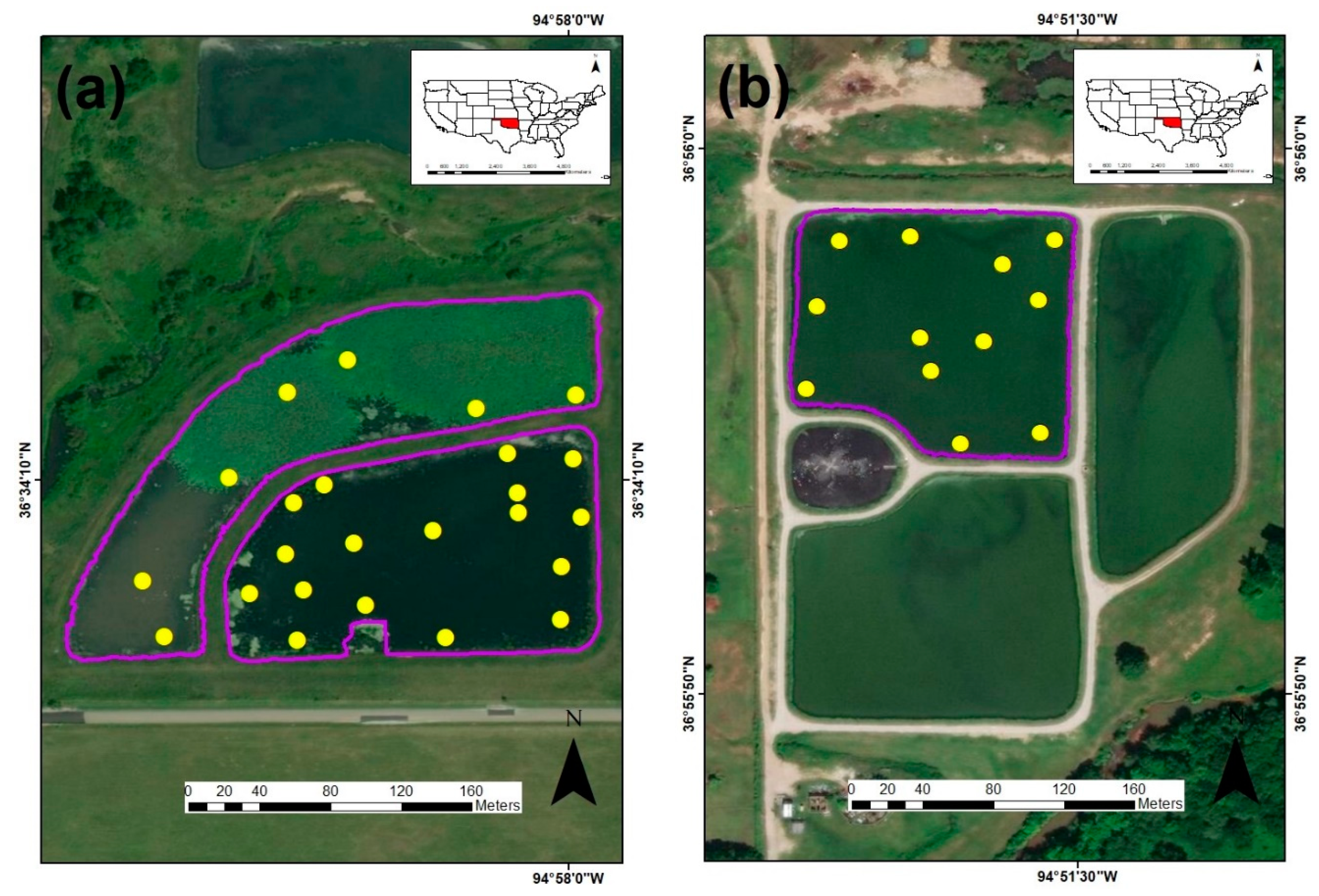
2.1. Study Areas
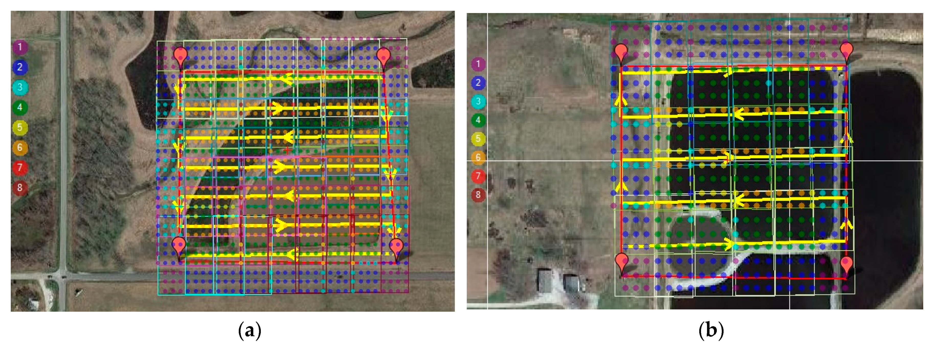
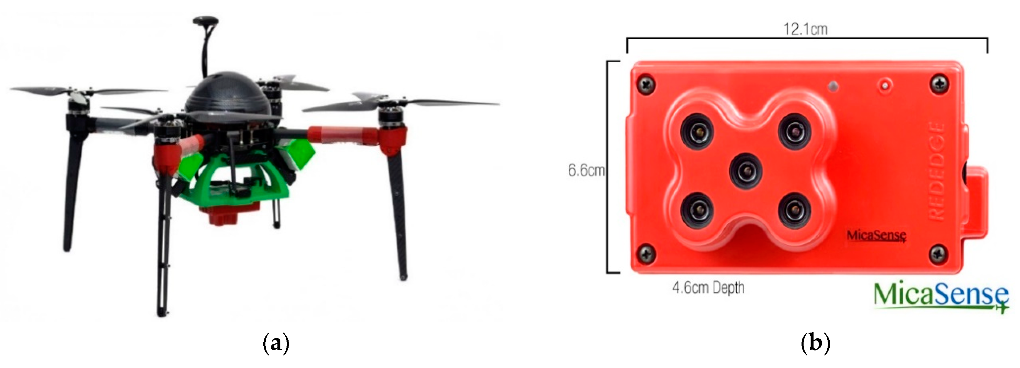
2.2. Water Quality and Multispectral Imagery Data Collection
2.3. Methodology
2.3.1. Data Collection
2.3.2. Data Processing
Laboratory Analysis
Reflectance Extraction
2.3.3. Model Development and Validation
3. Results
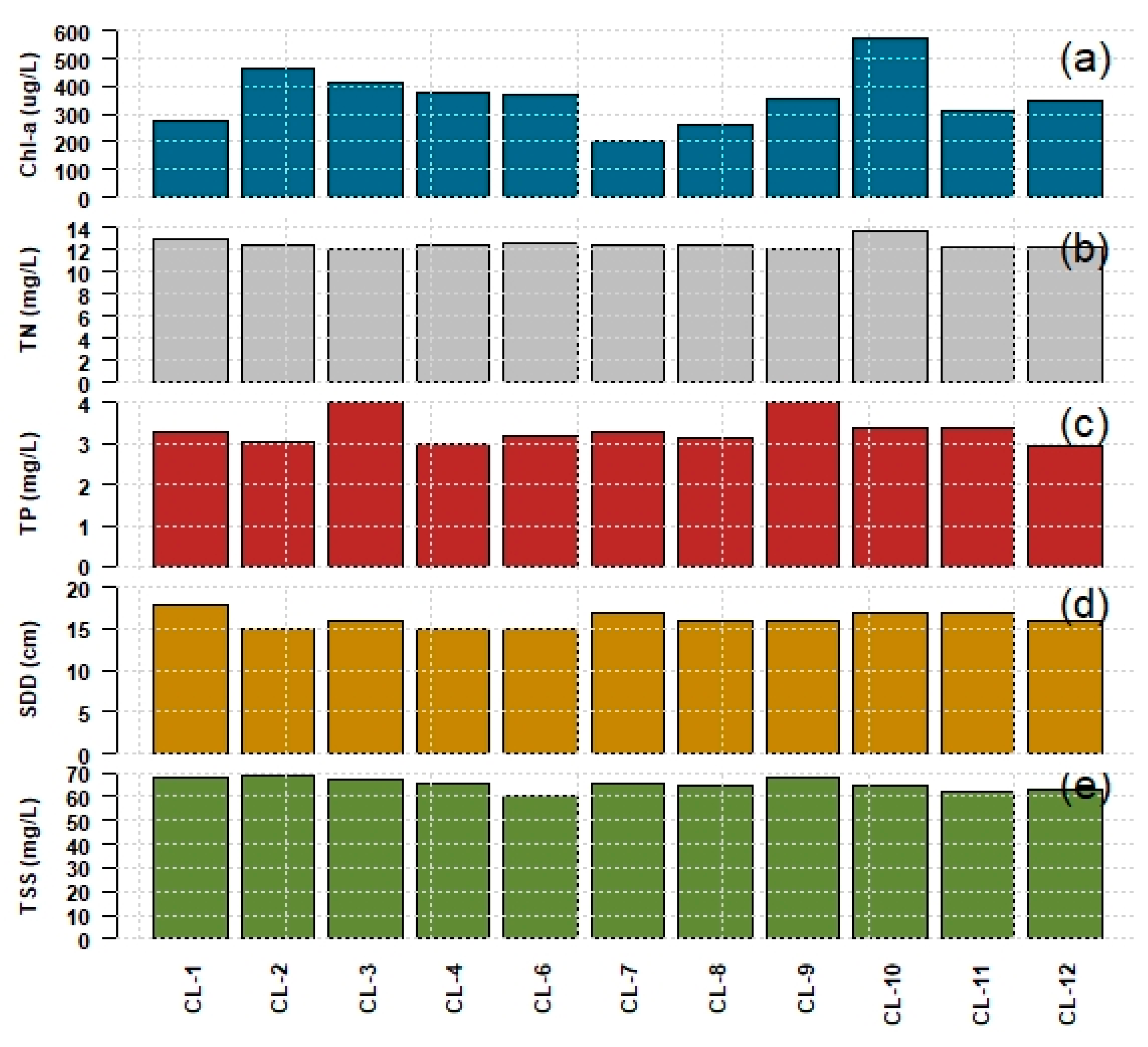
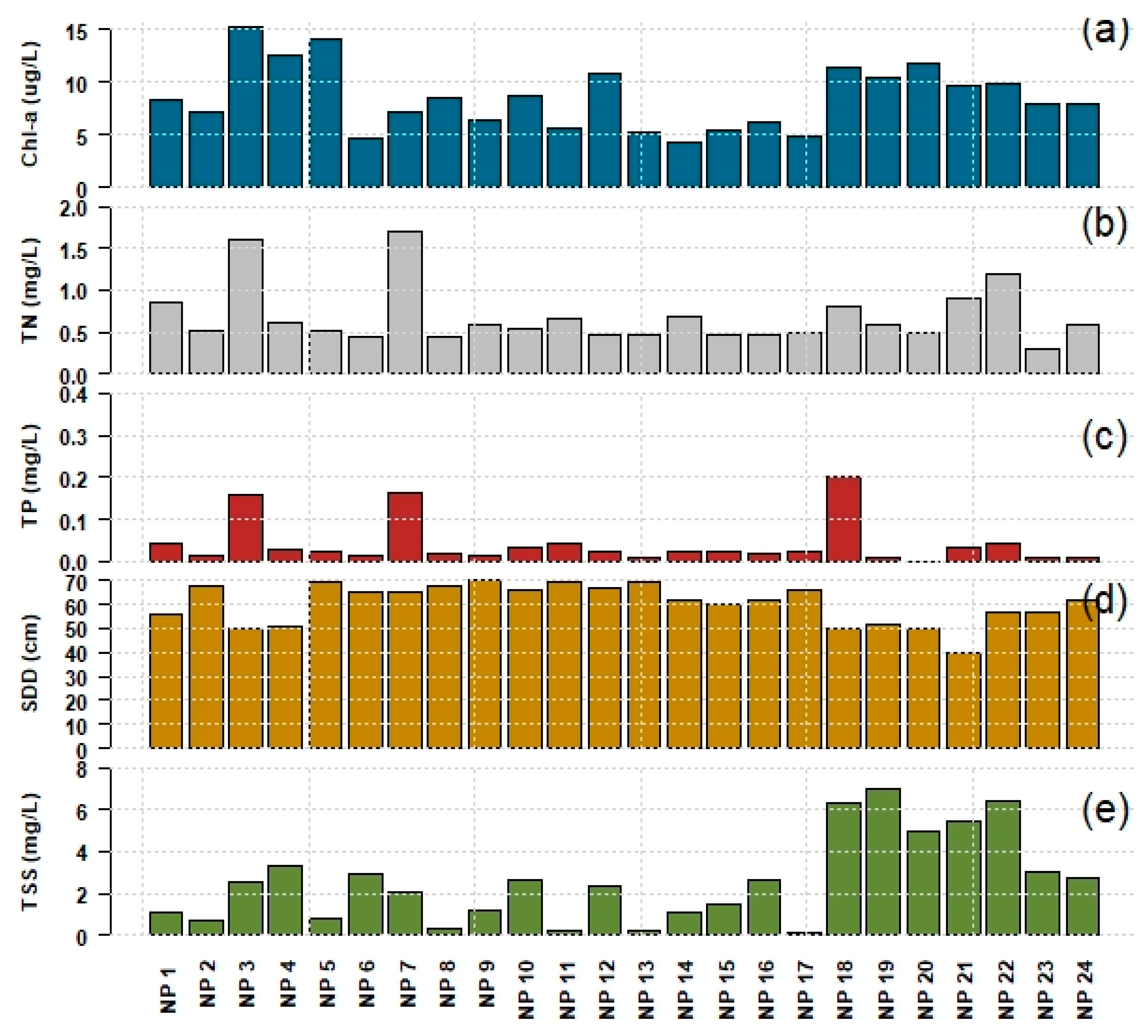
3.1. Water Quality
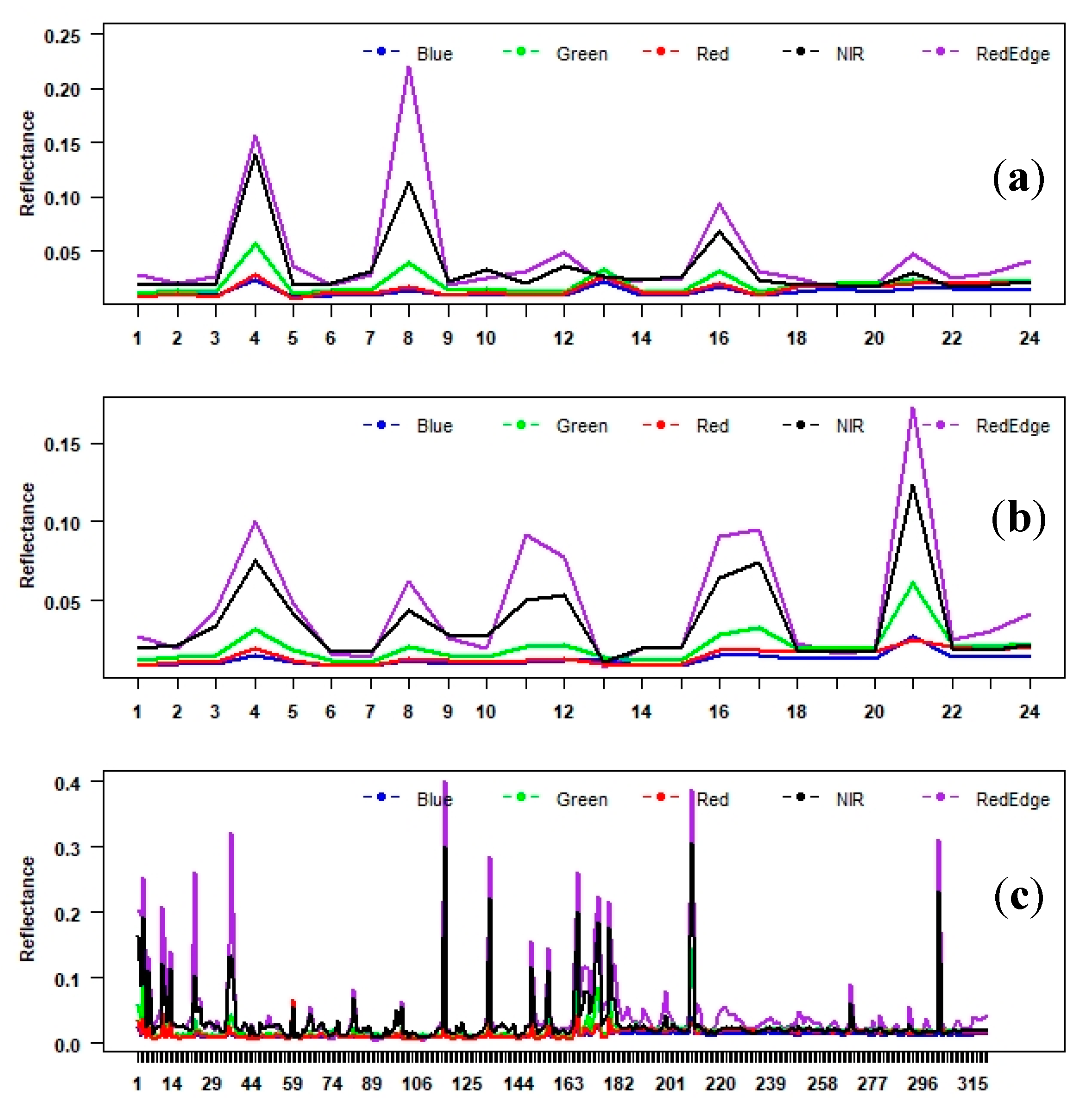
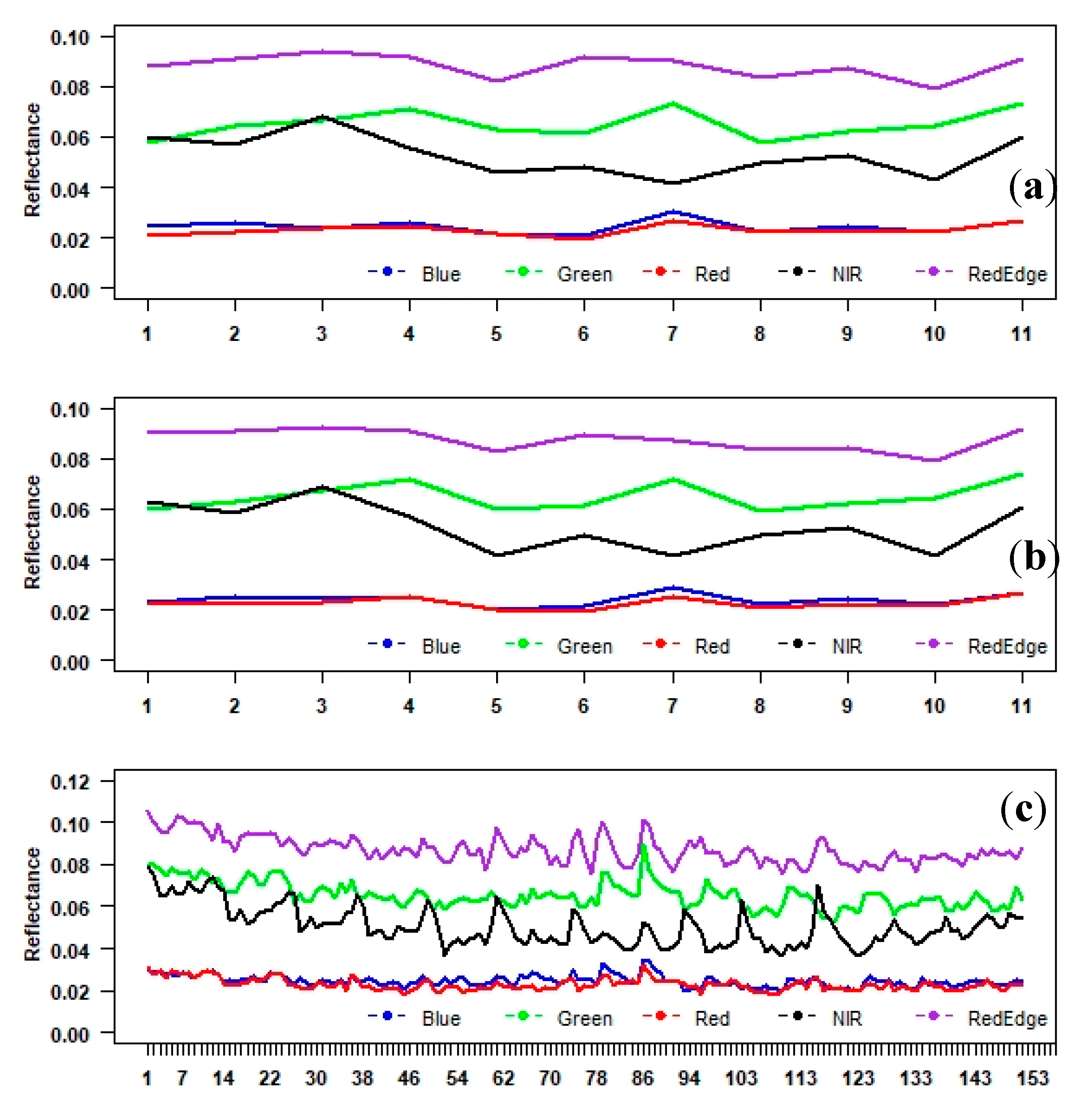
3.2. Reflectance Extraction
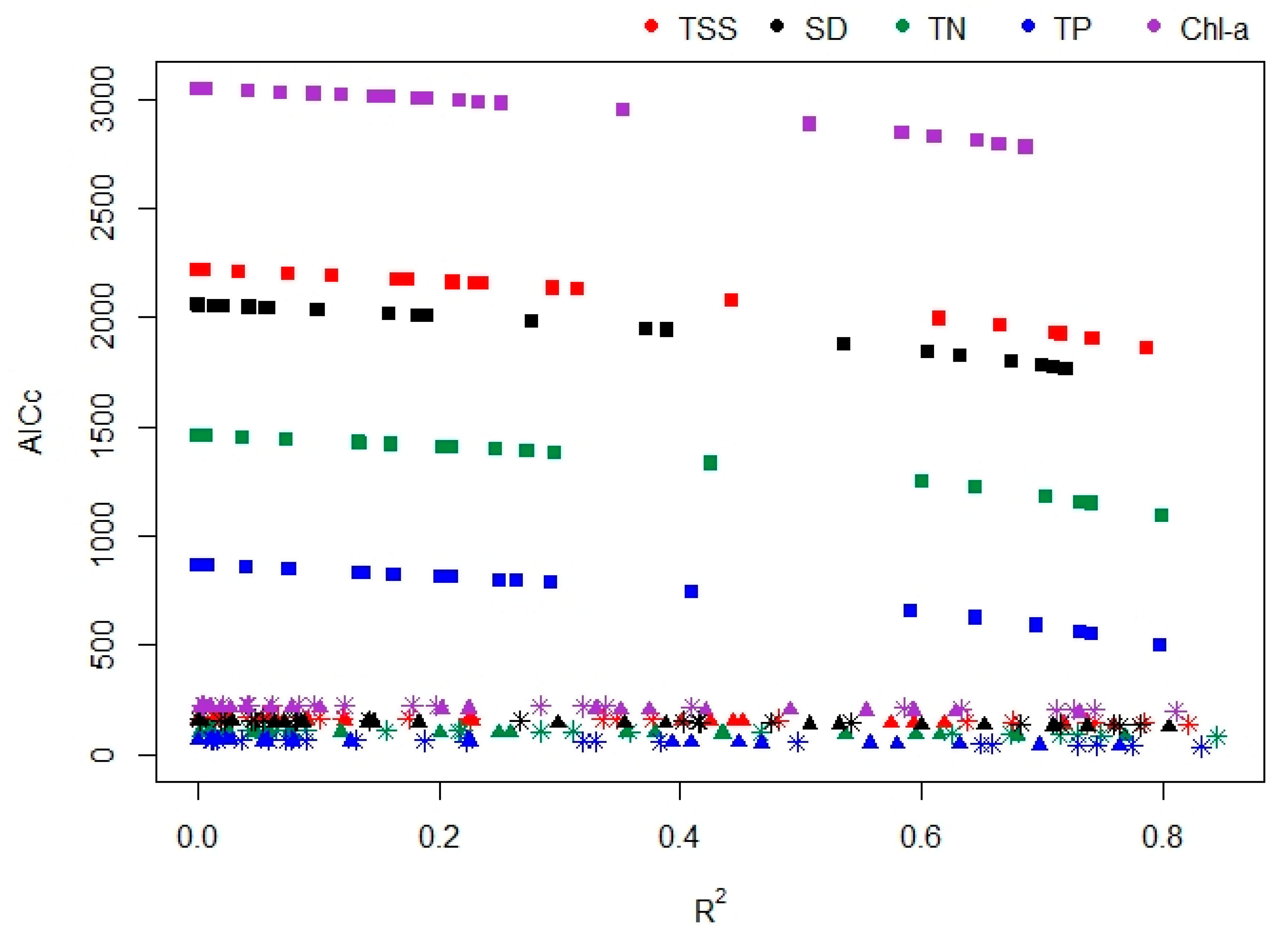
3.3. Models Development and Extraction Scenarios Evaluation
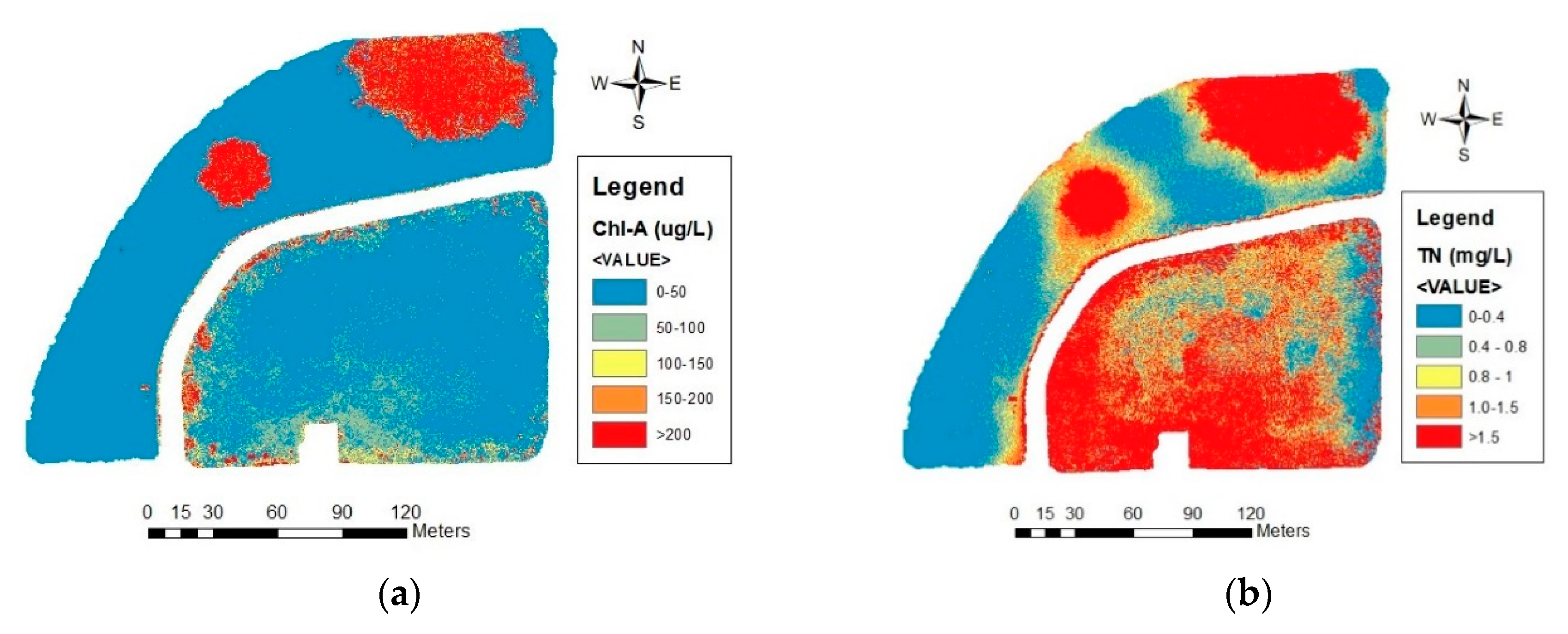
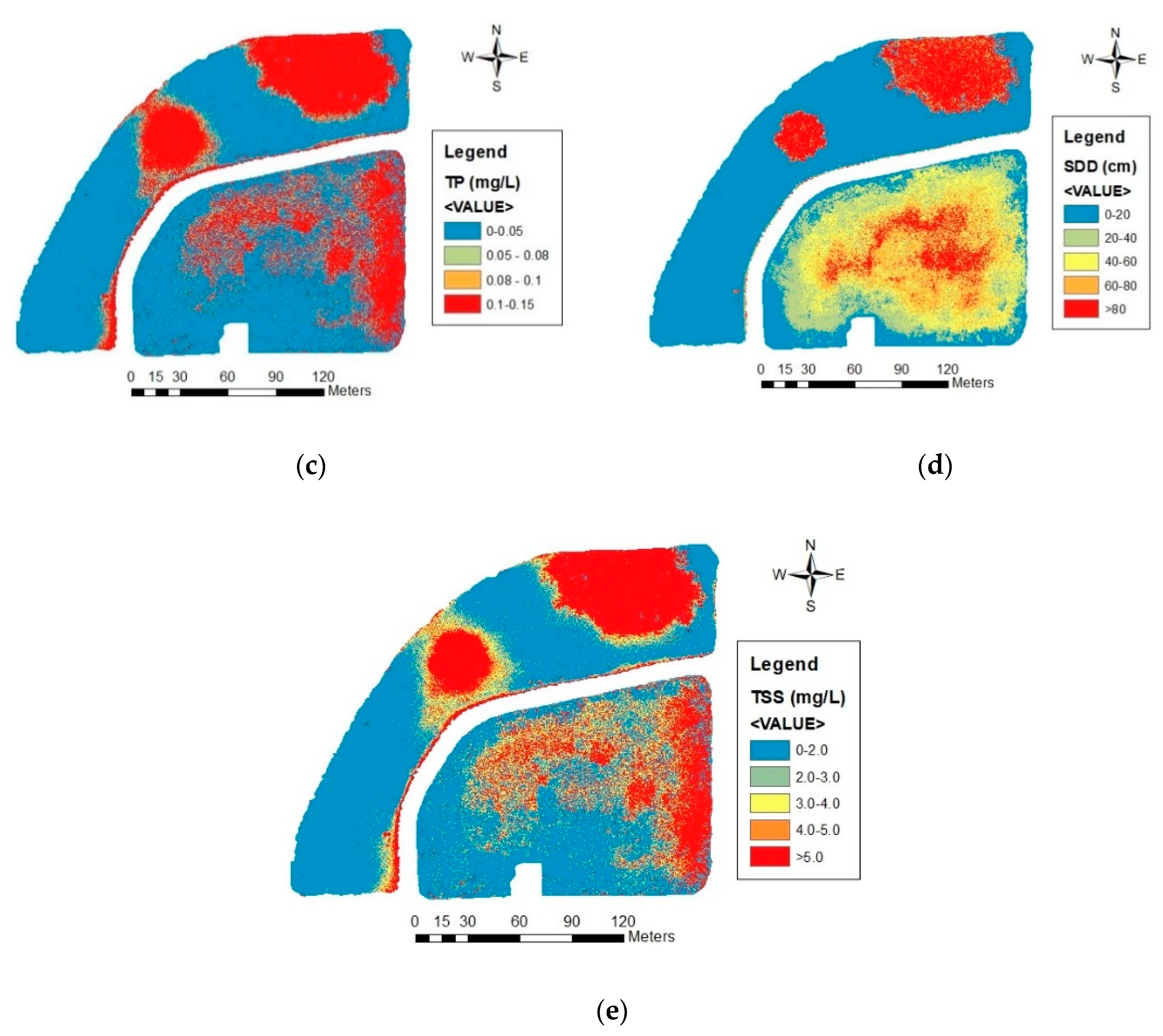
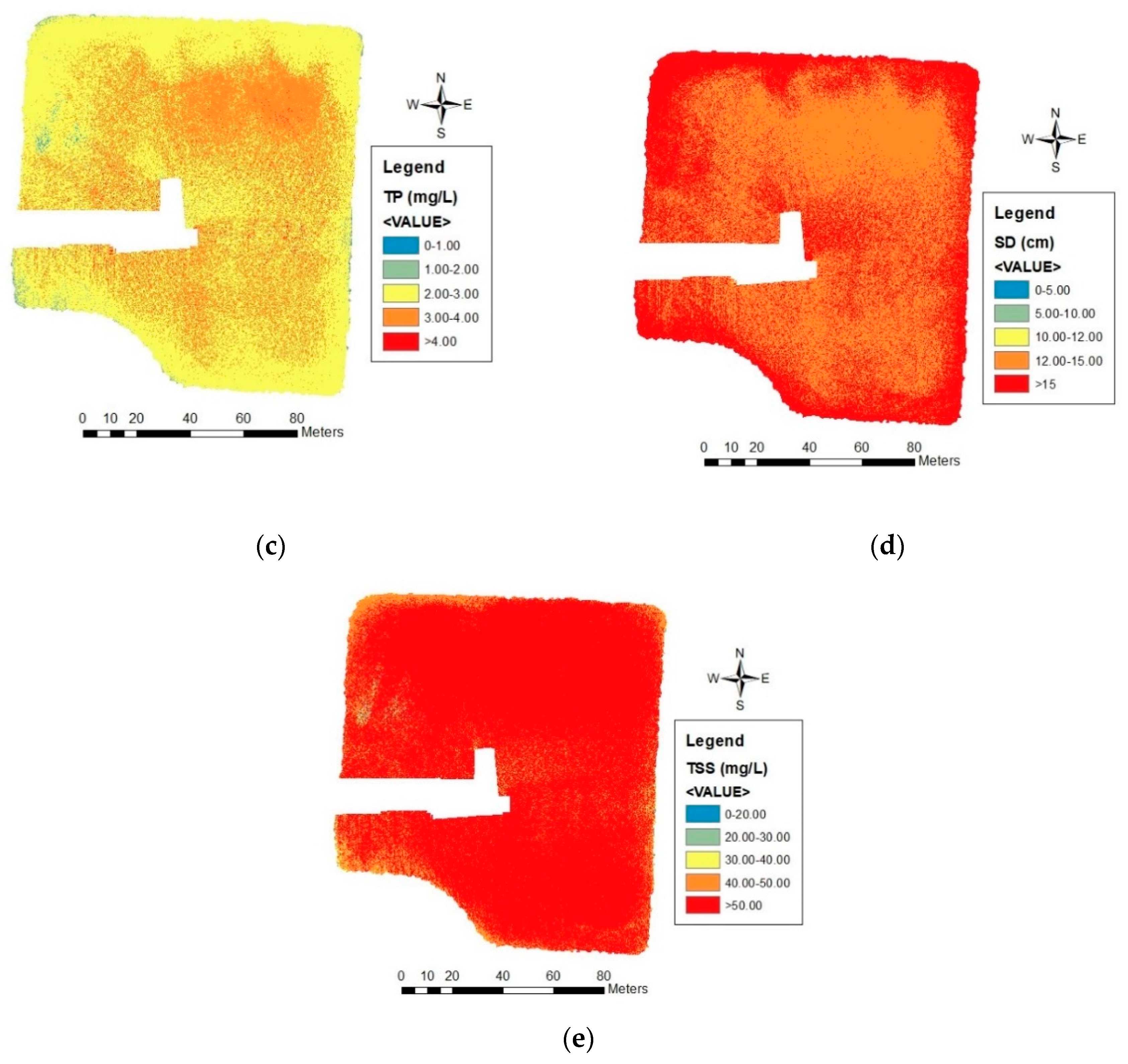
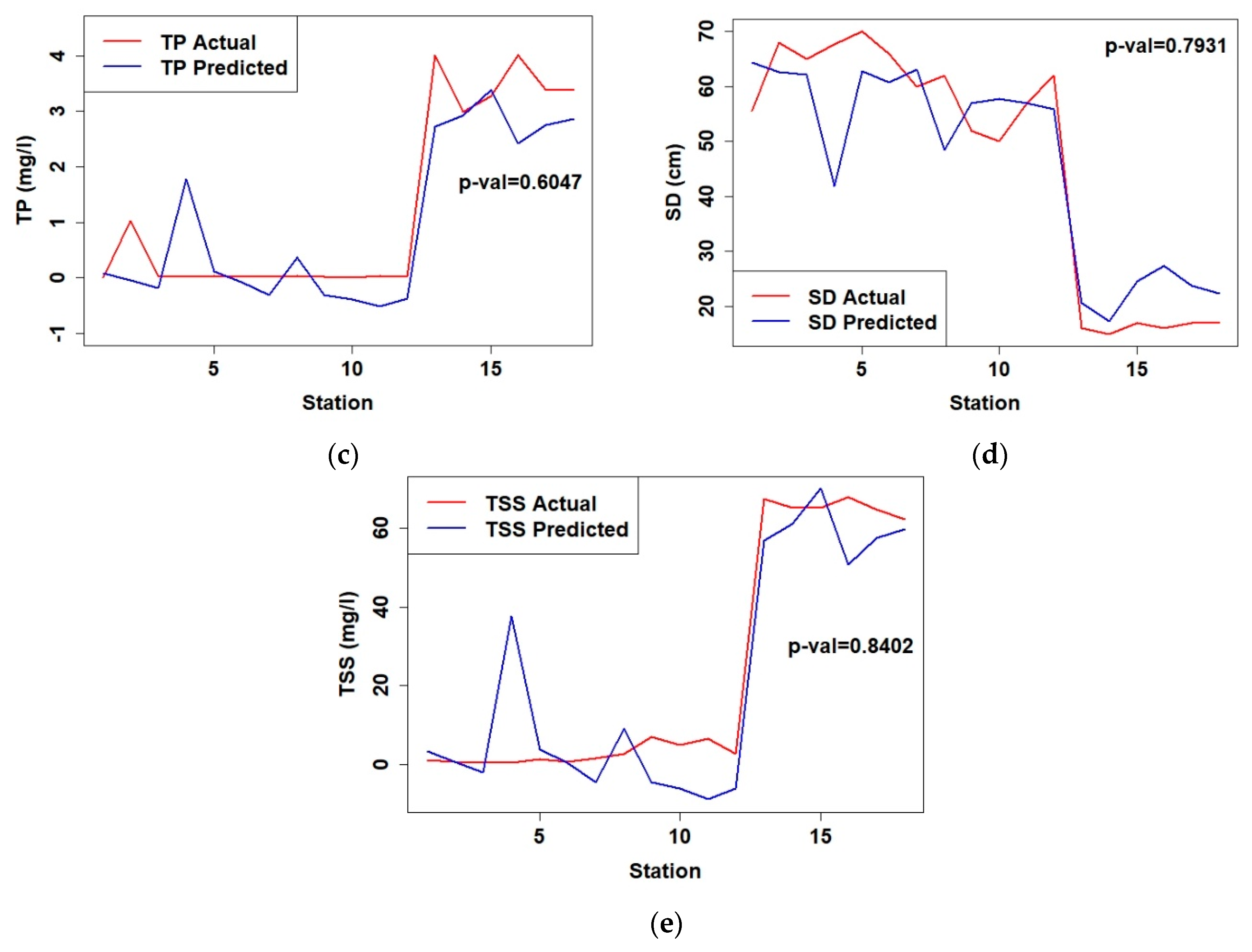
3.4. Validation and Spatial Distribution Maps
4. Discussion
5. Conclusions
Author Contributions
Funding
Acknowledgments
Conflicts of Interest
References
- United States Geological Survey. Measuring and Monitoring Water. Available online: https://www.usgs.gov/mission-areas/water-resources/science/measuring-and-monitoring-water (accessed on 10 December 2019).
- Wilde, F.D. Field Measurements: U.S. Geological Survey Techniques of Water-Resources Investigations. Available online: http://pubs.water.usgs.gov/twri9A6/ (accessed on 10 December 2019).
- Kloiber, S.M.; Brezonik, P.L.; Olmanson, L.G.; Bauer, M.V. A procedure for regional lake water clarity assessment using landsat multispectral data. Remote Sens. Environ. 2002, 82, 38–47. [Google Scholar] [CrossRef]
- Zhao, D.; Cai, Y.; Jiang, H.; Xu, D.; Zhang, W.; An, S. Estimation of water clarity in taihu lake and surrounding rivers using landsat imagery. Adv. Water Resour. 2011, 34, 165–173. [Google Scholar] [CrossRef]
- Ritchie, J.C.; Zimba, P.V.; Everitt, J.H. Remote sensing techniques to assess water quality. Am. Soc. Photogramm. Remote Sens. 2003, 6, 695–704. [Google Scholar] [CrossRef] [Green Version]
- Olmanson, L.G.; Bauer, M.E.; Brezonik, P.L. A 20-year landsat water clarity census of minnesota’s 10,000 lakes. Remote Sens. Environ. 2008, 112, 4086–4097. [Google Scholar] [CrossRef]
- Brezonik, P.L.; Olmanson, L.G.; Finlay, J.C.; Bauer, M.E. Factors affecting the measurement of CDOM by remote sensing of optically complex inland waters. Remote Sens. Environ. 2015, 157, 199–215. [Google Scholar] [CrossRef]
- Baban, S.J. Detecting water quality parameters in the norfolk broads, U.K., using landsat imagery. Int. J. Remote Sens. 2007, 14, 1247–1267. [Google Scholar] [CrossRef]
- Dominguez, J.A.; Chuvieco, E.; Sastre-Merlin, A. Monitoring transparency in inland water bodies using multispectral images. Int. J. Remote Sens. 2009, 30, 1567–1586. [Google Scholar] [CrossRef]
- Duan, H.; Ma, R.; Hu, C. Evaluation of remote sensing algorithms for cyanobacterial pigment retrievals during spring bloom formation in several lakes of east China. Remote Sens. Environ. 2012, 126, 126–135. [Google Scholar] [CrossRef]
- Matthews, M.W.; Bernard, S.; Robertson, L. An algorithm for detecting trophic status (chlorophyll-a), cyanobacterial-dominance, surface scums and floating vegetation in inland and coastal waters. Remote Sens. Environ. 2012, 124, 637–652. [Google Scholar] [CrossRef]
- Ma, J.; Qin, B.; Wu, P.; Zhou, J.; Niu, C.; Deng, J.; Niu, H. Controlling cyanobacteria blooms by managing nutrient ratio and limitation in large hyper-eutrophic lake: Lake Taihu, China. J. Environ. Sci. 2015, 27, 80–86. [Google Scholar] [CrossRef]
- Mobley, C.; Stramski, D.; Bissett, W.; Boss, E. Optical modeling of ocean waters: Is the Case 1–Case 2 classification still useful? Oceanography 2004, 17, 60–67. [Google Scholar] [CrossRef]
- Morel, A.; Belanger, S. Improved detection of turbid waters from ocean color sensors information. Remote Sens. Environ. 2006, 102, 237–249. [Google Scholar] [CrossRef]
- Forget, P.; Ouillon, S.; Lahet, F.; Broche, P. Inversion of reflectance spectra of nonchlorophyllous turbid coastal waters. Remote Sens. Environ. 1999, 68, 264–272. [Google Scholar] [CrossRef]
- Lee, Z.; Hu, C. Global distribution of Case-1 waters: An analysis from seawifs measurements. Remote Sens. Environ. 2006, 101, 270–276. [Google Scholar] [CrossRef]
- Kirk, J.T.O. Optical water quality—What does it mean and how should we measure it? J. Water Pollut. Control Fed. 1988, 60, 194–197. [Google Scholar]
- International Ocean-Colour Coordinating Group (IOCCG). Why the Ocean Color? The Societal Benefits of Ocean-Colour Technology; International Ocean Colour Coordinating Group (IOCCG): Dartmouth, NS, Canada, 2008; p. 141. [Google Scholar]
- International Ocean-Colour Coordinating Group (Ioccg). Earth Observations in Support of Global Water Quality Monitoring; International Ocean Colour Coordinating Group (IOCCG): Dartmouth, NS, Canada, 2018; p. 132. [Google Scholar]
- Lillesand, T.M.; Johnson, W.L.; Deuell, R.L.; Lindstrom, O.M.; Meisner, D.E. Use of landsat data to predict the trophic state of minnesota lakes. Photogramm. Eng. Remote Sens. 1983, 49, 219–229. [Google Scholar]
- Giardino, C.; Pepe, M.; Brivio, P.A.; Ghezzi, P.; Zilioli, E. Detecting chlorophyll, secchi disk depth and surface temperature in a sub-alpine lake using landsat imagery. Sci. Total. Environ. 2001, 268, 19–29. [Google Scholar] [CrossRef]
- Asner, G.P. Cloud cover in landsat observations of the brazilian amazon. Int. J. Remote Sens. 2010, 22, 3855–3862. [Google Scholar] [CrossRef]
- Nelson, S.; Soranno, P.A.; Spence Cheruvelil, K.; Batzli, S.; Skole, D.L. Regional assessment of lake water clarity using satellite remote sensing. Educ. J. Limnol. 2003, 32, 27–32. [Google Scholar] [CrossRef] [Green Version]
- Torbick, N.; Hu, F.; Zhang, J.; Qi, J.; Zhang, H.; Becker, B. Mapping chlorophyll-a concentrations in west lake, China using landsat 7 ETM+. J. Great Lakes Res. 2008, 34, 559–565. [Google Scholar] [CrossRef]
- Guan, X.; Li, J.; Booty, W.G. Monitoring lake simcoe water clarity using landsat-5 TM images. Water Resour. Manag. 2011, 25, 2015–2033. [Google Scholar] [CrossRef]
- Bonansea, M.; Rodriguez, M.C.; Pinotti, L.; Ferrero, S. Using multi-temporal landsat imagery and linear mixed models for assessing water quality parameters in río tercero reservoir (argentina). Remote Sens. Environ. 2015, 158, 28–41. [Google Scholar] [CrossRef]
- Colomina, I.; Molina, P. Unmanned aerial systems for photogrammetry and remote sensing: A review. ISPRS J. Photogramm. Remote Sens. 2014, 92, 79–97. [Google Scholar] [CrossRef] [Green Version]
- Rusnak, M.; Sladek, J.; Kidova, A.; Lehotsky, M. Template for high-resolution river landscape mapping using UAV technology. Measurement 2018, 115, 139–151. [Google Scholar] [CrossRef]
- Louhaichi, M.; Petersen, S.; Gomez, T.; Jensen, R.R.; Morgan, G.R.; Butterfield, C. Remote spectral imaging using a low cost sUAV system for monitoring rangelands. Adv. Remote Sens. Geo Inform. Appl. 2018, 1, 143–145. [Google Scholar] [CrossRef]
- Doughty, C.; Cavanaugh, K. Mapping coastal wetlands biomass from high resolution unmanned aerial vehicle (UAV) imagery. Remote Sens. 2019, 11, 540. [Google Scholar] [CrossRef] [Green Version]
- Melville, B.; Fisher, A.; Lucieer, A. Ultra-high spatial resolution fractional vegetation cover from unmanned aerial multispectral imagery. Int. J. Appl. Earth Obs. Geoinf. 2019, 78, 14–24. [Google Scholar] [CrossRef]
- Berni, J.A.; Zarco-Tejada, P.J.; Suarez, L.; Fereres, E. Thermal and narrowband multispectral remote sensing for vegetation monitoring from an unmanned aerial vehicle. IEEE Trans. Geosci. Remote Sens. 2009, 47, 722–738. [Google Scholar] [CrossRef] [Green Version]
- Nebiker, S.; Lack, N.; Abacherli, M. Light-weight multispectral UAV sensors and their capabilities for predicting grain yield and detecting plant diseases. Int. Arch. Photogramm. Remote Sens. Spat. Inf. Sci. 2016, XLI-B1, 963–970. [Google Scholar] [CrossRef]
- Su, T.; Chou, H. Application of multispectral sensors carried on unmanned aerial vehicle (UAV) to trophic state mapping of small reservoirs: A case study of tain-pu reservoir in Kinmen, Taiwan. Remote Sens. 2015, 7, 10078–10097. [Google Scholar] [CrossRef] [Green Version]
- Kageyama, Y.; Takahashi, J.; Nishida, M.; Kobori, B.; Nagamoto, D. Analysis of water quality in Miharu dam reservoir, Japan, using UAV data. IEEJ Trans. Electr. Electron. Eng. Jpn. 2016, 11, 183–185. [Google Scholar] [CrossRef]
- Anderson, C.R.; Berdalet, E.; Kudela, R.M.; Cusack, C.K.; Silke, J.; O’Rourke, E.; Dugan, D.; McCammon, M.; Newton, J.A.; Moore, S.K.; et al. Scaling up from regional case studies to a global harmful algal bloom observing system. Front. Mar. Sci. 2019, 6. [Google Scholar] [CrossRef]
- Schmale, D.G.; Ault, A.P.; Saad, W.; Scott, D.T.; Westrick, J.A. Perspectives on harmful algal blooms (HABs) and the cyberbiosecurity of freshwater systems. Front. Bioeng. Biotechnol. 2019, 7. [Google Scholar] [CrossRef] [PubMed] [Green Version]
- Carlson, R.E. A trophic state index for lakes. Limnol. Oceanogr. 1977, 22, 361–369. [Google Scholar] [CrossRef] [Green Version]
- Davis, T.W.; Stumpf, R.; Bullerjahn, G.S.; McKay, R.M.; Chaffin, J.D.; Bridgeman, T.B.; Winslow, C. Science meets policy: A framework for determining impairment designation criteria for large waterbodies affected by cyanobacterial harmful algal blooms. Harmful Algae 2019, 81, 59–64. [Google Scholar] [CrossRef] [PubMed]
- Mesonet. Local Conditions. Available online: https://www.mesonet.org/index.php/weather/local (accessed on 10 December 2019).
- Oklahoma Department of Environmental Quality. Lagoon Sewage Treatment Systems. Available online: https://www.deq.ok.gov/wp-content/uploads/environmental-complaints/Lagoon-.pdf (accessed on 10 December 2019).
- YSI Incorporated. 6-Serie Multiparameter Water Quality Sondes User Manual. Available online: https://www.ysi.com/File%20Library/Documents/Manuals/069300-YSI-6-Series-Manual-RevJ.pdf (accessed on 7 December 2019).
- United States Environmental Protection Agency. Methods for Chemical Analysis of Waters and Waste Waters; EPA/600/4-79/020 (NTIS PB84128677); U.S. Environmental Protection Agency: Washington, DC, USA, 2002.
- Aerial Technology International. ATI AgBOT Data Sheet. Available online: http://store.aerialtechnology.com/product/agbot-2/ (accessed on 7 December 2019).
- Mission Planner; Computer Software. ArduPilot Development Team. Available online: https://ardupilot.org/planner/ (accessed on 23 December 2019).
- Pix4Dmapper; Computer Software; Pix4D SA: Prilly, Switzerland, 2011.
- ArcMap; Computer Software; Environmental Systems Research Institute (ESRI): Redlands, CA, USA, 2012.
- Akaike, H. Information Theory and an Extension of the Maximum Likelihood Principle. In Proceedings of the 2nd International Symposium on Information Theory, Tsahkadsor, Armenia, 2–8 September 1971; Akadémiai Kiadó: Budapest, Hungary, 1973; pp. 267–281. [Google Scholar]
- Burnham, K.P.; Anderson, D.A. Model Selection and Multimodel Inference, 2nd ed.; Springer: New York, NY, USA, 2002; pp. 1–488. [Google Scholar]
- Shapiro, S.S.; Wilk, M.B. An analysis of variance test for normality (complete samples). Biometrika 1965, 52, 591–611. [Google Scholar] [CrossRef]
- R Core Team. R Computer Software; R Core Team: Vienna, Austria, 2017. [Google Scholar]
- Gholizadeh, M.H.; Melesse, A.M.; Reddi, L. A comprehensive review on water quality parameters estimation using remote sensing techniques. Sensors 2016, 16, 1298. [Google Scholar] [CrossRef] [Green Version]
- Lim, J.; Choi, M. Assessment of water quality based on landsat 8 operational land imager associated with human activities in Korea. Environ. Monit. Assess. 2015, 187, 384–401. [Google Scholar] [CrossRef]
- Wu, C.; Wu, J.; Qi, J.; Zhang, L.; Huang, H.; Lou, L.; Chen, Y. Empirical estimation of total phosphorus concentration in the mainstream of the qiantang river in China using landsat TM data. Int. J. Remote Sens. 2010, 31, 2309–2324. [Google Scholar] [CrossRef]
- Sharaf El Din, E.; Zhang, Y. Estimation of both optical and non-optical surface water quality parameters using landsat 8 OLI imagery and statistical techniques. J. Appl. Remote Sens. 2017, 11, 046008. [Google Scholar] [CrossRef]
- Liu, J.; Zhang, Y.; Yuan, D.; Song, X. Empirical estimation of total nitrogen and total phosphorus concentration of urban water bodies in China using high resolution IKONOS multispectral imagery. Water 2015, 7, 6551–6573. [Google Scholar] [CrossRef] [Green Version]
- Song, K.; Li, L.; Li, S.; Tedesco, L.; Hall, B.; Li, L. Hyperspectral remote sensing of total phosphorus (TP) in three central indiana water supply reservoirs. Water Air Soil Pollut. 2012, 223, 1481–1502. [Google Scholar] [CrossRef]
- Liu, X.; Chen, Y.; Chen, Y.; He, R. Optimization of earth observation satellite system based on parallel systems and computational experiments. J. Control Theory Appl. 2013, 11, 200–206. [Google Scholar] [CrossRef]
- Allan, M.G.; Hamilton, D.P.; Hicks, B.J.; Brabyn, L. Landsat remote sensing of chlorophyll-a concentrations in central north island lakes of New Zealand. Int. J. Remote Sens. 2011, 32, 2037–2055. [Google Scholar] [CrossRef]
- Mushtaq, F.; Nee Lala, M.G. Remote estimation of water quality parameters of himalayan lake (kashmir) using landsat 8 OLI imagery. Geocarto Int. 2017, 32, 274–285. [Google Scholar] [CrossRef]
- Zhang, C.; Kovacs, J.M. The application of small unmanned aerial systems for precision agriculture: A review. Precis. Agric. 2012, 12, 693–712. [Google Scholar] [CrossRef]
- Hicks, B.J.; Stichbury, G.A.; Brabyn, L.K.; Allan, M.G.; Ashraf, S. Hindcasting water clarity from landsat satellite images of unmonitored shallow lakes in the Waikato Region, New Zealand. Environ. Monit. Assess. 2013, 185, 7245–7261. [Google Scholar] [CrossRef]
- Barrett, D.C.; Frazier, A.E. Automated method for monitoring water quality using landsat imagery. Water 2016, 8, 257. [Google Scholar] [CrossRef] [Green Version]
- Mu, X.; Hu, M.; Song, W.; Ruan, G.; Ge, Y.; Wang, J.; Huang, S.; Yan, G. Evaluation of sampling methods for validation of remotely sensed fractional vegetation cover. Remote Sens. 2015, 7, 16164–16182. [Google Scholar] [CrossRef] [Green Version]


| Nursery Ponds | Wastewater Lagoons | ||||
|---|---|---|---|---|---|
| Site ID | Window (Minutes) | Site ID | Window (Minutes) | Site ID | Window (Minutes) |
| NP-1 | +17 | NP-13 | +151 | CL-1 | +22 |
| NP-3 | +33 | NP-14 | +154 | CL-2 | +38 |
| NP-4 | +46 | NP-15 | +161 | CL-3 | +47 |
| NP-5 | +58 | NP-16 | +198 | CL-4 | +57 |
| NP-6 | +67 | NP-17 | +210 | CL-5 | +68 |
| NP-7 | +78 | NP-18 | +216 | CL-6 | +79 |
| NP-2 | +86 | NP-19 | +226 | CL-7 | +86 |
| NP-8 | +101 | NP-20 | +347 | CL-8 | +97 |
| NP-9 | +111 | NP-21 | +360 | CL-9 | +108 |
| NP-10 | +121 | NP-22 | +370 | CL-10 | +114 |
| NP-11 | +131 | NP-23 | +379 | CL-11 | +125 |
| NP-12 | +144 | NP-24 | +389 | CL-12 | +130 |
| Analyte | Method |
|---|---|
| Chlorophyll α | EPA 445.0 |
| Total Phosphorus | SM 4500-P J |
| Total Nitrogen | SM 4500-P J |
| Total Suspended Solids | EPA 160.2 |
| Oligotrophic System | Eutrophic System | |||||||||
|---|---|---|---|---|---|---|---|---|---|---|
| Mean | Median | SD | Min | Max | Mean | Median | SD | Min | Max | |
| Chl-a | 8.52 | 8.10 | 3.08 | 4.26 | 15.37 | 358.3 | 352.60 | 103.36 | 200.40 | 575.80 |
| TN | 0.68 | 0.56 | 0.35 | 0.30 | 1.71 | 12.47 | 12.40 | 0.47 | 12.00 | 13.60 |
| TP | 0.04 | 0.02 | 0.05 | 0.01 | 0.20 | 3.33 | 3.27 | 0.37 | 2.94 | 4.02 |
| SDD | 60.4 | 62.00 | 8.18 | 40.00 | 70.00 | 16.18 | 16.00 | 0.98 | 15.00 | 18.00 |
| TSS | 2.44 | 2.57 | 2.09 | 0.11 | 7.00 | 65.33 | 65.20 | 2.7 | 60.20 | 68.83 |
| WQP | Single Variable Model | R2 | Multiple Variable Model | R2 |
|---|---|---|---|---|
| SDD | =m*Green) + b | 0.781 | =m*(Blue/Red) – m*(Green/Red) + m*(Green/Blue) − b | 0.888 |
| TSS | =m*(Green/Red) − b | 0.821 | =m*(Blue/Red) – m*(Green/Red) + m*(Green/Blue) + b | 0.987 |
| TN | =m*(Green/Red) − b | 0.845 | =m*(Blue/Red) – m*(Green/Red) – m*(Green/Blue) + b | 0.979 |
| TP | =m*(Green/Red) − b | 0.832 | =m*(Blue/Red) – m*(Green/Red) + m*(Green/Blue) + b | 0.984 |
| Chl-a | =m*(Green/Red) − b | 0.810 | =m*(Green) – m*(Red) + b | 0.846 |
| WQP | Green | Red | y-Intercept (b) | |||
|---|---|---|---|---|---|---|
| Slope (m) | ||||||
| SDD | 164.32 | 108.33 | 78.67 | -- | -- | 61.91 |
| TSS | 264.5 | 148.2 | 185.2 | -- | -- | 215.3 |
| TN | 45.43 | 26.16 | 32.94 | -- | -- | 36.92 |
| TP | 12.441 | 6.993 | 8.810 | -- | -- | 9.953 |
| Chl-a | -- | -- | -- | 9158.79 | 13,359 | 27.99 |
| Satellite | Spatial Resolution | Temporal Resolution (Day) |
|---|---|---|
| Landsat–5 | 30 m | 16 |
| Landsat–7 | 30 m | 16 |
| Landsat–8 | 30 m | 16 |
| QuickBird–2 | 15 m | 1–3 |
| Orb View–3 | 4 m | 3 |
| Gaofen–1 | 8 m | 4 |
| Sentinel–2 | 10 m | 5 |
| sUAS | 0.06–0.08 m | Flight-specific |
© 2019 by the authors. Licensee MDPI, Basel, Switzerland. This article is an open access article distributed under the terms and conditions of the Creative Commons Attribution (CC BY) license (http://creativecommons.org/licenses/by/4.0/).
Share and Cite
Arango, J.G.; Nairn, R.W. Prediction of Optical and Non-Optical Water Quality Parameters in Oligotrophic and Eutrophic Aquatic Systems Using a Small Unmanned Aerial System. Drones 2020, 4, 1. https://doi.org/10.3390/drones4010001
Arango JG, Nairn RW. Prediction of Optical and Non-Optical Water Quality Parameters in Oligotrophic and Eutrophic Aquatic Systems Using a Small Unmanned Aerial System. Drones. 2020; 4(1):1. https://doi.org/10.3390/drones4010001
Chicago/Turabian StyleArango, Juan G., and Robert W. Nairn. 2020. "Prediction of Optical and Non-Optical Water Quality Parameters in Oligotrophic and Eutrophic Aquatic Systems Using a Small Unmanned Aerial System" Drones 4, no. 1: 1. https://doi.org/10.3390/drones4010001
APA StyleArango, J. G., & Nairn, R. W. (2020). Prediction of Optical and Non-Optical Water Quality Parameters in Oligotrophic and Eutrophic Aquatic Systems Using a Small Unmanned Aerial System. Drones, 4(1), 1. https://doi.org/10.3390/drones4010001