Article

Multi-Sensor UAV Tracking of Individual Seedlings and Seedling Communities at Millimetre Accuracy

1
ARC Centre for Mine Site Restoration, School of Molecular and Life Sciences, Curtin University, Kent Street, Bentley, WA 6102, Australia
2
Spatial Sciences, School of Earth and Planetary Sciences, Curtin University, Kent Street, Bentley, WA 6102, Australia
*
Author to whom correspondence should be addressed.
Drones 2019, 3(4), 81; https://doi.org/10.3390/drones3040081
Submission received: 6 September 2019 / Revised: 22 October 2019 / Accepted: 28 October 2019 / Published: 30 October 2019
(This article belongs to the Special Issue Ecological Applications of Drone-Based Remote Sensing)

Abstract

:
The increasing spatial and temporal scales of ecological recovery projects demand more rapid and accurate methods of predicting restoration trajectory. Unmanned aerial vehicles (UAVs) offer greatly improved rapidity and efficiency compared to traditional biodiversity monitoring surveys and are increasingly employed in the monitoring of ecological restoration. However, the applicability of UAV-based remote sensing in the identification of small features of interest from captured imagery (e.g., small individual plants, <100 cm2) remains untested and the potential of UAVs to track the performance of individual plants or the development of seedlings remains unexplored. This study utilised low-altitude UAV imagery from multi-sensor flights (Red-Green-Blue and multispectral sensors) and an automated object-based image analysis software to detect target seedlings from among a matrix of non-target grasses in order to track the performance of individual target seedlings and the seedling community over a 14-week period. Object-based Image Analysis (OBIA) classification effectively and accurately discriminated among target and non-target seedling objects and these groups exhibited distinct spectral signatures (six different visible-spectrum and multispectral indices) that responded differently over a 24-day drying period. OBIA classification from captured imagery also allowed for the accurate tracking of individual target seedling objects through time, clearly illustrating the capacity of UAV-based monitoring to undertake plant performance monitoring of individual plants at very fine spatial scales.

1. Introduction

Ecological restoration and other recovery activities directed at returning ecological functioning to degraded ecosystems, is being undertaken at increasing scale around the world [1,2,3]. It is being increasingly recognised that humans must achieve a net gain in the extent and function of indigenous ecosystems in coming decades if ambitious global targets relating to sustainable development and biodiversity preservation are to be met [1,4,5]. However, ecological restoration is a complex process and achieving desired restoration trajectories requires significant planning, careful and targeted on-ground activities and detailed subsequent monitoring and adaptive management over long time periods [4,6,7]. The monitoring of ecological recovery projects such as ecological restoration is particularly important, both to ensure that predetermined goals are being met and to inform adaptive management in situations where trajectories are unsatisfactory [4,8,9]. Many studies have utilised keystone plant species (e.g., species of notable abundance or importance to ecological functioning) as indicators to project restoration trajectory [9,10]. However, the demand for more rapid and accurate methods of predicting restoration trajectory continues to grow with the increasing spatial and temporal scales of ecological recovery projects [1,2,3,11]. Unmanned Aerial Vehicles (UAVs) have increasingly been applied to meet this demand, as they offer greater cost-efficiency and ease of use, increased spatial and temporal resolution and improved rapidity and safety compared to traditional biodiversity monitoring surveys [12,13].
One area of particularly strong uptake in UAV-based monitoring in in the monitoring of post-mining rehabilitation and ecological restoration [14]. Many mining operations are located in relatively remote regions and post-mining landforms are often steep, unstable or hazardous to traverse on foot (e.g., waste rock landforms and tailings storage facilities). UAVs offer an effective monitoring solution for these landforms, on which rehabilitation or ecological restoration are often regulatory requirements [15,16], as their operation avoids human exposure to hazardous conditions, can access areas not able to be monitored on foot and does not risk degrading or trampling sensitive or regenerating communities [17]. Additionally, UAVs do not pose a pathogen transmission risk in areas where soil- or water-borne pathogens such as dieback (Phytopthora spp.; [18]) represent a serious threat to ecological recovery and to the integrity of natural communities. The ability of UAVs to fly at extremely low altitudes, coupled with lower operating costs and minimal infrastructure requirements, yields more accessible and cost-efficient data capture at far greater spatial resolution than can be achieved by manned aircraft or satellites [19].
Higher spatial resolution greatly improves the accuracy of automatic image classification techniques such as Object-Based Image Analysis (OBIA; a technique that splits each image into spectrally similar ‘objects,’ which allows for classification not just on colour but other factors like shape, size and relationship to surrounding objects [20]) and supervised machine learning (a process that “teaches” a program what set classes are meant to look like by providing training examples; based off of the given examples, the program then classifies the remaining images by their similarity to the specified classes [21]). Very high spatial resolution is a prerequisite where monitoring goals require the identification of small features of interest (e.g., individual plants) [20,22]. The mining industry are increasingly seeking monitoring tools that provide accurate and reliable assessments of restorative trajectories [14,23] and studies have identified examinations of growth, phenology and physiological performance in restored communities at the level of individual plants as a crucial desired component of this toolbox [16,24,25].
As UAVs can carry a variety of sensors and multiple sensors can be mounted on a single platform to capture data simultaneously in a single flight [26], they represent an increasingly appropriate tool for monitoring plant performance. UAVs are widely employed in the monitoring of plant health and performance in the agricultural sector [27], with recent studies demonstrating their effective application to the estimation of leaf carotenoid content in vineyards [28], the identification of nitrogen stress in maize [29], the monitoring of crop pests [30], in assessments of leaf area index in wheat [31], in the diagnosis of various ailments such as sheath blight in rice [32] and in assessments of water stress in barley fields [33] and olive orchards [34]. Many of these applications employed multispectral sensors, due primarily to their ability to provide early warning of plant stressors at a relatively affordable price point compared to other, more advanced sensors such as hyperspectral or thermal cameras [35]. Multispectral sensors can detect near-infrared (NIR) light, which affords the ability to monitor various multispectral indices (e.g., Normalised Difference Vegetation Index, NDVI) that can show changes in plant health before any visible signs appear [36]. The use of multispectral imagery to improve classification accuracy has been previously demonstrated at larger scales in dry forest and peat bogs [20,37], to classify trees and shrubs on the basis of plant health [20] and to provide early warning of plant stress in plantation trees [38]. Indeed, the addition of multispectral cameras to automated image classification processes broadly may represent an opportunity to markedly increase the accuracy of target plant object classification. More advanced sensors such as thermal and hyperspectral sensors are likely to significantly improve this capability, as multispectral sensors do not provide adequate data to determine the reason for observed plant performance declines due to limited spectral resolution [39]. Determining the causes of observed declines is important to action correct management and at least in agricultural crop species requires the spectral resolution offered by hyperspectral sensors and classification accuracies nearing 100% have been achieved when using hyperspectral sensors to differentiate between three different fungal diseases in sugar beets [40] and in detecting head blight in wheat [41]. Additionally, thermal sensors offer a highly accurate tool for assessing water stress in vegetation [33,42,43,44] and have also been applied variously in the monitoring of mammalian fauna [45,46,47]. The use of thermal and other UAV-mounted sensors in fauna monitoring is likely to increase to meet the growing demands for more rapid and reliable assessments of fauna biodiversity and behaviour [11]. However, the use of more advanced sensors remains predominantly constrained by cost [14], as thermal and hyperspectral sensors are currently between three to twelve times more expensive than multispectral sensors [35] and translational research from agriculture to the monitoring of ecological restoration projects has to date been broadly restricted to the use of multispectral sensors (e.g., the identification and mapping of woody vegetation cover in post-mining revegetation [48]). Translational research has not yet tested the potential of UAVs to monitor heterogenous natural vegetation communities at very fine spatial scales and is yet to demonstrate that plant health and performance can be monitored at the scale of individual plants or that establishment and development can be reliably tracked at the seedling stage when plants are most vulnerable to environmental stressors [49].
This study aimed to utilise the fine-scale spatial and temporal resolution offered by UAV-mounted sensors to identify target seedlings and track and assess their growth and development from a simple background community on representative restoration substrates. Target seedlings can be identified with a high level of accuracy from RGB imagery using OBIA [50] and multispectral imagery works well in automated image classification approaches as the extra information provided allows users to split classification classes not only by species but by level of plant health based off of multispectral indices [20]. We utilised a UAV equipped with both RGB and multispectral cameras to monitor a juvenile plant community over a period of drying to track individual target seedling objects (Lupinus angustifolia) through time and simultaneously gathered data to assess surrogate measures of their ecophysiological performance using a variety of visible and multispectral indices over the course of the drying period to contrast the performance of target seedlings with co-occurring non-target seedlings (co-occurring grasses). Given the often remote and poorly accessible nature of post-mining landforms, we examined whether naturally occurring reference points (local points with defining features that can be located repeatable throughout the data series, that is, small landscape features such as rocks and soil surface microtopography) could be used as common reference points to align orthomosaics produced from images captured by different sensors or on different days. Our objective was to achieve high level of accuracy in the identification, counting and tracking of individual target seedling objects through relative referencing between image captures to facilitate monitoring of a desired area of interest, not to achieve a high level of precision in determining the absolute spatial positioning of target individuals. We hypothesised that target and non-target seedling objects would exhibit different spectral signatures (e.g., different values for visible and multispectral vegetation indices, as surrogates for ecophysiological performance) and that these signatures would respond differently over the drying period facilitating the discrete monitoring of both groups. Additionally, we hypothesised that pre-drying plant performance (determined from values from visible and multispectral indices) would be a significant predictor of the speed of seedling mortality during the drying period.

2. Materials and Methods

2.1. Study Site

The study was conducted at the University of Western Australia Shenton Park Field Station, Perth, Western Australia (31°56′55″ S, 115°47′39″ E). UAV flights were undertaken over a 400 m2 trial area divided into four experimental 100 m2 plots (10 m × 10 m) with different surface treatments representing generalised restoration substrates in Western Australia (Figure 1). Surface treatments included a ‘control’ of undisturbed local sandy soil (smooth, homogenous texture and light background colour) representative of typical post-mining substrate in Banksia woodland restoration [16]; a ‘textured’ treatment of undisturbed local sandy soil with scattered crushed overburden rock (2–20 cm in size, giving increased surface heterogeneity) used to rock armour the slopes of restoration landforms [51]; a ‘dark’ treatment of undisturbed local sandy soil capped with a 1 cm layer of tailings generated from the processing of magnetite ore [52]; and a ‘high red-ratio’ treatment of undisturbed local sandy soil capped with a 1 cm layer of red clay loam soil from a mine site in the Midwest region of Western Australia [51]. All capping materials were sourced from a major magnetite mining operation located approximately 400 km northeast of Perth, Western Australia. Additionally, to examine whether seed and seedling detection rates were affected by surface topography, half of each treatment plot was manually ripped to a depth of 20 cm using a backhoe (Figure 1) to mimic standard ripping practices in post-mining restoration [16].
Plots were seeded in September 2017, split into three seeding sub-treatments representing increasing volumes of broadcast seeds (and, correspondingly, increasing seedling density; Figure 1). The seed mix broadcast included seeds of a target species, Lupinus angustifolia L. (Fabaceae), in a commercial grass species mix comprising Festuca arundinacea Schreb. and Stenotaphrum secundatum (Walter) Kuntze (Poaceae). The target species was selected as its seeds were large (ca. 1 cm) and distinctly coloured (white) and its distinctive large, dark green palmate leaves produced from a central stem provided a strong comparison with the small linear leaves of non-target grasses. The seed mix was intended to represent a potential post mining restoration scenario where monitoring was required for a species of restoration interest with large, distinctly coloured seeds and distinctive foliage (e.g., Banksia species, where seeds have been polymer coated [53]) among a matrix of grassy invasive weeds (a situation common in regional restoration initiatives [16]). The seed mix was broadcast at three densities: low, comprising 15 L. angustifolia seeds and 50 grass seeds per m−2; medium, comprising 25 L. angustifolia and 250 grass seeds per m−2; and high, comprising 50 L. angustifolia and 1000 grass seeds per m−2. In total, 12000 L. angustifolia seeds were broadcast. Plots were irrigated daily for a 10-week growing season before the irrigation was turned off and soils were allowed to dry for a further four weeks. Daily weather information, as well as daily climatic variable data used in analyses, were retrieved from the Bureau of Meteorology’s Swanbourne station, ID 009215 (located ca. 2 km from the study site).

2.2. Flights and Image Capture

Manual flights of the study site were conducted daily (5 metre flight altitude) for 14 weeks using a DJI Phantom 4 Pro (Dà-Jiāng Innovations, Shenzhen, China) equipped with a 20 Megapixel RGB camera and a Parrot Sequoia multispectral camera (only for flights in weeks 9 through 14). Flights were conducted manually due to the small area surveyed and low flight altitudes. All flights were conducted with front- and sidelap of 70% and at low speeds (approximately 3 kph) to avoid image blur. Flights were conducted at the same time each day (early morning, approximately 8.30 am once shadows from adjacent trees no longer fell over the trial area), with the exception of the last week of the experiment when increasing aggression from local avifauna required flights to be conducted at random times throughout the day in an attempt to avoid interactions (see Section 4.5).

2.3. Image Analysis

JPG images from all UAV flights were merged together using the Agisoft Photoscan software, to produce RGB (from the phantom 4 pro integrated camera) and multispectral (from the sequoia) rectified orthomosaics as well as Digital Elevation Models (DEMs) for each flight. The final resolution of RGB orthomosaics was 1.02 mm per pixel and of multispectral orthomosaics was 4.64 mm per pixel. Images were locally geo-referenced and naturally occurring reference points (local points with defining features that can be located repeatable throughout the data series, that is, small landscape features such as rocks and soil surface microtopography) were used as common reference points to align orthomosaics produced from images captured by different sensors or on different days. Orthomosaic alignment thus aimed to facilitate ‘identification accuracy’ of target seedling objects and the discrete tracking of individual target seedling objects through time, rather than to attain high levels of absolute ‘spatial accuracy’ in terms of global positioning.

2.4. Monitoring of Plant Response to Water Stress

Ten weeks after seeding, the irrigation to the trial plot was switched off and the soil was left to dry for four weeks. During this period, the plot was monitored with the Phantom 4 Pro and the Parrot Sequoia multispectral camera in order to track response of target and non-target seedlings to water stress. Due to operational difficulties with the multispectral camera, inclement weather and interaction with an aggressive native raptor, successful flights were conducted on 12 out of the 24 days during the drying period. Following all flights, orthomosaics and DEMs were generated from both the Phantom 4 Pro’s RGB imagery and the Parrot Sequoia multispectral imagery. Orthomosaics and DEMs were created in Agisoft Photoscan, with the Sequoia imagery requiring initial reflectance calibration from its reflectance target (conducted in Photoscan). Orthomosaics were split into four discrete images representing the four different surface covers and QGIS was used to manually align RGB and multispectral orthomosaics for analysis. However, a lack of identifiable feature objects resulted in insufficient alignment for dark, red and control treatments, a challenge that was made more problematic by the reduced spatial resolution of the multispectral sensor. Only the textured treatment could be aligned with an acceptable level of accuracy, with scattered waste rock providing sufficiently distinct features for georeferencing. While target seedling objects were generally well-aligned, occasional misalignment by a few centimetres occasionally resulted in image objects derived from RGB imagery having minimal overlap with image objects derived from multispectral imagery (Figure 2). Following alignment of RGB and multispectral orthomosaics in QGIS, the orthomosaics were imported into eCognition.
Automated identification of target seedlings from captured imagery was initially undertaken using OBIA (utilising orthomosaics and DEMs generated from RGB imagery from a single point in time, with no post-processing alignment required) captured imagery from day 68, after a period of seven consecutive days in which no new seedlings were scored in any treatment. Seedlings were identified by an initial multiresolution segmentation, in which all objects with a green ratio above a set threshold were assigned to the ‘target’ class, followed by additional refining of the rule set using Hue-Saturation-Intensity (HIS [54]) transformations, Triangular Greenness Index (TGI), area (of the object, in cm2), compactness [54], height (represented by the mean difference to neighbour objects in the DEM; see Reference [50]), perimeter/width and length/width. Full rule sets used in analyses and example outputs, are presented in Reference [50]. For each image, the total leaf cover of non-target grass seedlings (including false positive seedling identifications) was determined for all objects not already classified using green ratio and TGI. Following target seedling identification, a report was generated from each orthomosaic showing key colour indices of each image object, tracking features including green ratio, TGI, Visible Atmospheric Resistant Index (VARI), Normalised Difference Vegetation Index (NDVI), Soil-Adjusted Vegetation Index (SAVI) and area (of the object, in cm2). Equations and rationale for all visible and multispectral indices are provided in Table 1.

2.5. Tracking of Specific Individuals

From RGB imagery captured on day 68, 25 individual target seedling objects were randomly selected for individual plant performance monitoring. Orthomosaics from day 68 to day 92 were trimmed to only the Textured treatment and the QGIS georeferencer plugin was used to align all future orthomosaics to the coordinates of the day 68 orthomosaic. Target seedlings were identified initially based off of their green ratio, with generous thresholds (see Supplementary 1 for ruleset) used to allow for continued identification even as green ratio of plants changed in response to drying conditions. Following identification via green ratio, each of the chosen 25 target seedlings were identified from their GPS co-ordinates. Following the identification of a target seedling from imagery of the first day of drying, the north-, east-, south- and west- most points were identified and GPS coordinates of each recorded. In future imagery, seedlings were identified as being the seedling of interest if the GPS position of the object’s centroid fell within the previously identified extremities. Full rulesets are presented in Supplementary 1. A report was generated from each orthomosaic showing key colour indices of each individual target seedling object, tracking features including area, green ratio, TGI and VARI. Only visible spectrum indices were calculated for the 25 tracked individual target seeding objects, due to georeferencing and overlap errors with multispectral imagery.

2.6. Statistics

To determine whether the spectral signature of the monitored plant community varied in response to climatic conditions, linear regression models were fitted to determine the effect of daily climatic variables (rainfall, solar exposure, maximum temperature and minimum temperature) on each of the visible spectrum (TGI, VARI and Green Ratio) and multispectral (NDVI and SAVI) indices utilised. All data were square root transformed prior to multiple linear regression analyses to meet assumptions of normality (assessed by Shapiro-Wilk tests of normality) and homogeneity of variances (as assessed by Levene’s test for equality of variances).
To determine whether classified target and non-target seedling object groups exhibited discrete spectral signatures, two-way mixed ANOVA were employed to determine whether mean object area and visible spectrum and multispectral indices varied significantly among the two groups over the experimental period using Greenhouse-Geisser estimates of epsilon (ε) as assumptions of sphericity were not met (SPSS Statistics 25, IBM, United States). Simple main effects among classified object groups at each time point were determined using Tukey post hoc tests.
Two-tailed Pearson correlations were run to determine which visible spectrum or multispectral index provided the strongest association with declines in the target seedling object community (mean object area and number of surviving individuals).
For analyses, the 25 tracked target seedling objects were binned into four size categories on the basis of object area at day 68: small (<50 cm2), medium (50–100 cm2), large (100–150 cm2) and very large (>150 cm2). To determine whether different sized target seedling objects exhibited different spectral signatures in response to drying conditions, two-way mixed ANOVA were employed to determine whether mean object area and visible spectrum indices varied significantly among the four groups over the experimental period using Greenhouse-Geisser estimates of ε as assumptions of sphericity were not met (SPSS Statistics 25, IBM, United States). Simple main effects among classified object groups at each time point were determined using Tukey post hoc tests.
Data are presented as mean ± standard error, unless otherwise stated.

3. Results

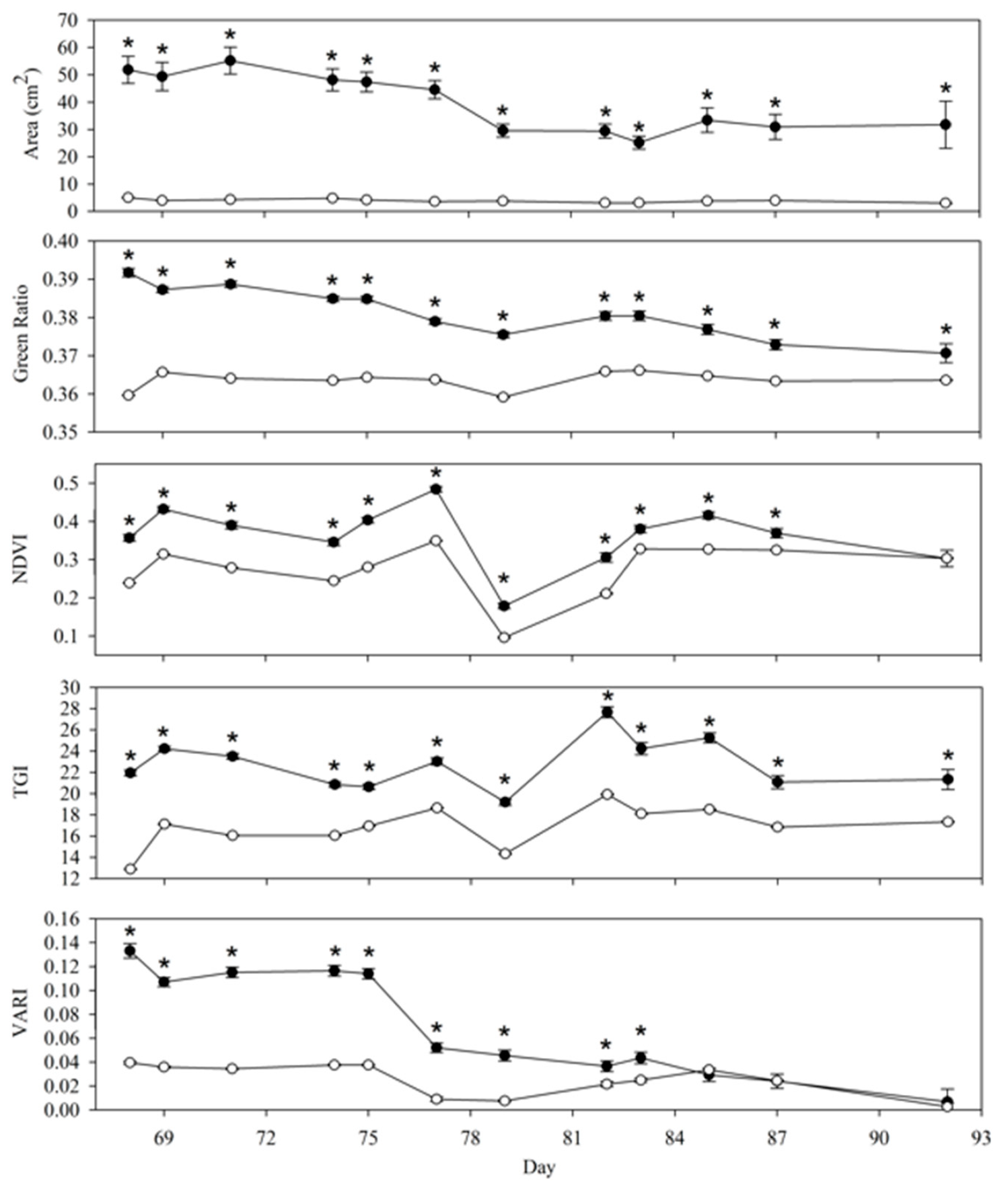
3.1. Response of Spectral Signature to Climatic Conditions

Mean object area and both visible spectrum and multispectral indices were significantly predicted by daily climatic variables (Table 2), with strongest effect sizes of regression models evident for multispectral indices (NDVI and SAVI) followed by green-dependent visible spectrum indices (TGI and green ratio). Regression coefficients and standard errors for all multiple regression analyses are presented in Table 3. Object area, TGI, VARI and green ratio were negatively associated with daily temperatures and solar exposure and positively associated with rainfall, while NDVI and SAVI were positively associated with all climatic variables.

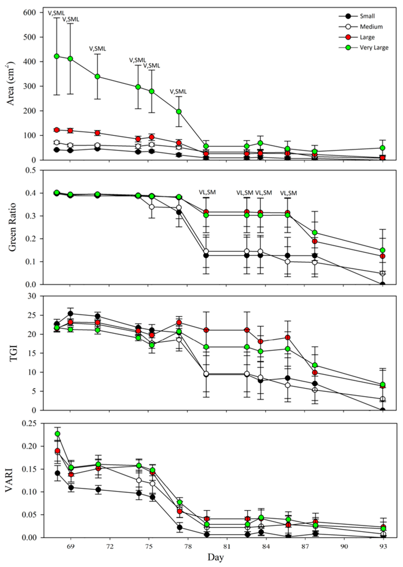
3.2. Plant Performance Monitoring for Target and Non-Target Seedling Communities

OBIA classification identified 156 target seedling objects with a total area of 0.8 m2 and 10,419 non-target seedling objects with a total area of 5.2 m2 from day 68 imagery. The number and total area of both target and non-target seedling objects declined rapidly over the 24-day drying period. By day 92, only 14 target seedling objects with a total area of 0.04 m2 (reductions of 91 and 94%, respectively) and 16,585 non-target seedling objects with a total area of 1.7 m2 (reductions of 47 and 68%, respectively) could be identified.
Classified target seedling objects exhibited distinct spectral signatures from that of non-target seedling objects and these signatures responded differently to the 24-day drying period (Figure 3). There was a statistically significant interaction between all measured indices and time among groups (Table 4), with target objects ca. 10-fold larger than non-target objects and exhibiting higher values for Green Ratio, Normalised Difference Vegetation Index (NDVI), Soil-adjusted Vegetation Index (SAVI), Triangular Green Index (TGI) and Visible Atmospherically-resistant Index (VARI) over the experimental period. Mean values for all measured spectral indices declined for both target and non-target seedling objects over the 24-day drying period. The area, green ratio and TGI of target seedling objects remained significantly higher than that of non-target objects, while values of NDVI, SAVI and VARI for the two groups gradually trended to similarity (Figure 3).
VARI and Green Ratio were moderately positively correlated with both mean object area and the number of target individuals over the monitoring period (Table 5), while NDVI and SAVI correlated moderately with mean object area but poorly with the number of target individuals. TGI exhibited no correlation with either variable.

3.3. Monitoring Individual Target Seedling Objects through Time

A total of 16 naturally occurring reference points (all small rocks) were used to align orthomosaics, ranging in size from 4.9–161.1 cm2 (average 44 ± 11.2). Following orthomosaic alignment, OBIA classification allowed for the tracking of the designated 25 target seedling objects (individuals) over the 24-day drying period with a high level of accuracy and precision. The centroids of target seedling objects exhibited global average X- and Y-axis displacement from their initial recorded position of 10 ± 0.9 mm and 14 ± 1.1 mm, respectively, over the 24-day monitoring period, with the greatest centroid displacement being 66 mm (Table 6). No statistically significant correlation was evident between the area of target individuals and either X- (R2 = 0.017, P = 0.937) or Y- (R2 = 0.095, P = 0.651) centroid displacement.
At the beginning of the drying period (day 68) the 25 target seedling objects ranged in Area from 33–982 cm2 (mean 150 ± 40.3 cm2; Table 6). Object area and all visible spectrum indices declined rapidly in monitored target individuals over the 24-day drying period (Figure 4), even following a 17 mm rainfall event over days 80–83 (Supplementary 2). The number of days until mortality ranged from 7–24 (mean 16 ± 1.3) across all classes and decreased along a size gradient from Very Large (19 ± 2.8 days; n = 5) and Large (18 ± 2.3 days; n = 6) individuals to Medium (13 ± 2.2 days; n = 8) and Small (12 ± 2.2 days; n = 6) individuals.
Individuals from Very large and Large size classes generally exhibited higher mean values for all metrics over the experimental period, although classes were statistically similar in all metrics by day 92 (Figure 4). There were statistically significant interactions between the area of classified groups and time (F[3.592, 25.144] = 5.877, P = 0.002, partial η2 = 0.456, ε = 0.120) and the Green Ratio of classified items and time (F[7.381, 51.666] = 0.1.164, P = 0.339, partial η2 = 0.143, ε = 0.246), while neither TGI (F[6.966, 48.786] = 1.399, P = 0.227, partial η2 = 0.167, ε = 0.232) nor VARI (F[9.814, 52.516] = 0.795, P = 0.602, partial η2 = 0.102, ε = 0.250) interacted significantly with time among groups.

4. Discussion

4.1. The Effect of Daily Climatic Conditions on Spectral Indices

The strong influence of daily weather conditions on spectral indices indicates that these metrics provided a useful measure for plant response to weather conditions. Images were calibrated with the aid of a reflectance target to control for the effect of daily climatic variance on reflectance values, as the ratio of reflectance of various wavelengths of light determine the values of vegetation indices utilised [57]. Weather-dependent variation in indices was therefore reflective of changes in the spectral signature of seedlings in response to factors such as moisture, wind and temperature [59]. Object area and green-dependent visible spectrum indices (TGI, VARI and green ratio), which are considered indicators of leaf chlorophyll content [55,56], increased in periods of higher soil moisture following rainfall and decreased with higher daily temperatures and solar irradiance. Previous studies suggest that higher leaf chlorophyll content during such favourable periods for growth would be expected [60,61,62]. NDVI and SAVI were positively associated with all climatic variables but declined towards the end of the experiment for L. angustifolia when drought stress was likely greatest, reflecting their utility as general indicators of plant health [57]. However, field study of plant physiological responses to stress factors such as water limitation and temperature should ideally be conducted concomitantly to validate the collection of spectral data [14,63]. Future studies should continue translational research to test the utility of spectral indices currently applied in agricultural settings to assessment of the health of non-agricultural plant species and communities and complement remote sensing data with ground truthing examination of plant ecophysiological performance.

4.2. Classification and Tracking of Seedling Communities

Target and non-target seedlings exhibited distinctly different visible-spectrum and multispectral signatures, differed statistically significantly in every spectral index examined and their spectral signatures behaved differently over the course of the drying phase of the experiment (Figure 3). These differences allowed for the discrete and accurate tracking of object groups both spatially and temporally and for the measurement of spectral index values as indicators of plant performance independently for each group. This study also provides the first evidence that accurate and reliable UAV-based monitoring of plant health is achievable not only at fine scales for establishing seedling communities but also at the scale of individual seedlings. Although our data were collected from low-altitude flights and from a constrained spatial area, they demonstrate the significant capability that UAVs will likely bring to the monitoring of ecological restoration and rehabilitation, as well as other industries such as silviculture and viticulture [64,65], with further research and development.
Application of this capability to ecological recovery monitoring could dramatically improve the accuracy and rapidity of surveys for particular species of interest in large-scale restoration plantings (e.g., spectral discrimination of a particular rare or restoration-significant species from among a biodiverse reinstated plant community) and improve the capacity to monitor plant performance at individual-scale to enable early warning of declining plant health (e.g., to identify declines in high-value or indicator species enabling early responsive restoration management). Although UAVs are likely to represent an effective monitoring tool for many restoration and rehabilitation projects, there are two major constraints to be overcome. The first is legislative restrictions, which cannot be discussed in depth due to differing laws from jurisdiction to jurisdiction and the second is cost, which remains a primary limitation to UAV application and the specific technological requirements of UAV-based remote sensing in ecological recovery are likely to differ among projects dependent upon their ecological recovery goals and monitoring outcomes. With adequate investment and demand-driven research UAVs almost certainly represent the future of monitoring in ecological recovery [14].
Studies have suggested that satellite-based remote sensing may facilitate accurate and real-time monitoring of plant health at community and landscape scale [66]. Given the more rapid turnaround times offered by UAVs compared with satellite imagery and the current application of UAVs to plant performance monitoring in agricultural contexts [43,67], we suggest that accurate real-time monitoring of plant health in ecological restoration using UAVs may already be possible with current technology and infrastructure. As the availability of only low-resolution sensors constrained our experimentation to low-altitude flights, future studies should also test the outcomes of multi-sensor UAV-based plant performance monitoring at greater flight altitudes and with higher resolution sensors. Additionally, studies should focus on testing a broader array of multispectral (and, indeed, hyperspectral) indices and robustly testing the relevance of these indices to the physiological performance of monitored plants.

4.3. Classification and Tracking of Individual Seedlings

The use of naturally occurring reference points yielded acceptable accuracy in orthomosaic alignment and undertaking OBIA on aligned orthomosaics allowed for precise tracking of specific individual seedlings over the 24-day drying period. Locational errors were low, with object centroid displacement for tracked objects averaging <15 mm across all objects over the course of the experiment. This precision allowed individual seedlings to be tracked as they developed, while simultaneously capturing a range of ecological data relating to their growth and performance, until mortality was evident (confirmed by ground-truthing). To our knowledge this is the first time that UAV-based imagery has been empirically demonstrated to offer such fine-scale spatial and temporal resolution in monitoring plant growth and development. While we acknowledge that our study was conducted over a small area and using imagery captured at very low altitudes, our data offer compelling evidence that UAV-based remote sensing can generate meaningful, reliable and affordable empirical data about the growth and development of vegetation communities and even individual plants early in their life cycle. This capacity can only be improved by the application of more technologically advanced UAV systems (e.g., multi-sensor platforms and sensors offering greater resolution or greater spectral discrimination) and may revolutionize the manner in which the monitoring of environmental recovery activities such as rehabilitation and ecological restoration are undertaken. UAV-based aerial monitoring of rehabilitated or restored areas offers an accurate method of tracking seedling communities and even high-value individuals (e.g., rare, threatened or commercially-important species), providing practitioners with a robust tool for predicting the trajectory of these communities by remotely measuring growth and development and providing early warning signs of environmental stressors such as drought.

4.4. Sensor Misalignment

One factor reducing the utility of multispectral imagery captured in this study was poor overlap for target seedlings among captured RGB and multispectral imagery. This misalignment likely reflected a lack of synchronisation between the drone-mounted RGB camera and the multispectral sensor; although both sensors were capturing an image every two seconds, images were not captured simultaneously. Images for each sensor were thus captured at slightly different points in space, causing overlap error at the scale of several millimetres. This reduced the accuracy of individual object locations within resultant orthomosaics, yielding internal target object misalignment within even perfectly aligned orthomosaics. This error could be resolved through development of a combined single-unit RGB and multispectral sensor able to be triggered simultaneously and geotagged by the same GPS unit. Although the multispectral sensor we utilised does house an integrated RGB camera, it offered reduced resolution (16 megapixel) and possessed a rolling shutter (rather than the global shutter used on the Phantom 4 Pro). Rolling shutters can reduce orthomosaic accuracy and resolution by introducing significant image distortion from imagery taken from a moving platform such as a UAV [68]. We echo previous calls for urgent emphasis to be placed upon the development of affordable and reliable multi-sensor pods capable of triggering all sensors simultaneously and being tagged by the same GPS unit to eliminate or reduce error [14]. Further consistency and accuracy in image capture locations could be achieved through the use of real-time kinematic (RTK) GPS units, which are able to hold planned flightpaths to within centimetre-level tolerances [69]. Accuracy and precision in object location and target overlap among imagery can also be improved through the use of numerous ground control points (GCPs) [42]. GCPs allow for more accurate alignment than reliance upon fixed surface features (e.g., rocks, infrastructure) such as those employed in this study. However, in scenarios such as the monitoring of ecological restoration on post-mining landforms the placement and use of traditional GCPs may be impractical due to limited site accessibility, hazardous features (e.g., unconsolidated tailings storage facilities) or rugged terrain (e.g., angle of repose slopes on waste rock landforms). While sensor output alignment will likely be improved in the future, our data suggest that even small naturally occurring reference points can be an effective tool for relative orthomosaic alignment.

4.5. Avian Interactions with the UAV

Studies should report significant fauna interactions during UAV use to better understand their impact as environmental monitoring tools. Significant interactions during our experiment were observed with multiple individuals of Australian Black-Shouldered Kites, Elanus axillaris. These raptors conducted multiple shallow dives towards the UAV while it was in flight, beginning in early December and becoming increasingly frequent over the latter days of the trial. Visual surveys were conducted prior to all flights and flights did not proceed if a Black-Shouldered Kite was sighted. The UAV was immediately landed following any approach by a bird, with flights terminated for the rest of the day and no physical contact was made at any point between the UAV and the birds. One other interaction of note was of Australian Magpies, Cracticus tibicen, which often flew or landed underneath the UAV while it was in flight. These birds appeared unperturbed by the presence of the UAV and were regularly present in imagery captured from flights undertaken at 5 and 15 metre altitude (see Supplementary Materials).

5. Conclusions

This study provides evidence for the significant utility of UAV-based sensing of both visible and non-visible vegetation indices in monitoring individual target seedlings within seedling communities at fine spatial scales. OBIA classification effectively and accurately discriminated among target and non-target seedling objects and these groups exhibited distinct spectral signatures (six different visible-spectrum and multispectral indices) that responded differently over a 24-day drying period. OBIA classification from captured imagery also allowed for the accurate tracking of individual target seedling objects through time, clearly illustrating the capacity of UAV-based monitoring to undertake plant performance monitoring of individual plants at very fine spatial scales. The strongest effect sizes of regression models assessing among-group differences in spectral signature were obtained for multispectral indices (NDVI and SAVI) and green-dependent visible spectrum indices (TGI, VARI and green ratio) and these metrics were also informative for tracking individual seedlings through time. We propose that these indices represent a useful tool for plant performance assessment and discretionary classification in the context of rehabilitation and ecological restoration but that they will likely require significant further development to be as informative for native plants as they currently are in agricultural settings. With further research and investment UAV-based remote sensing will allow industry and restoration practitioners to undertake plant performance monitoring earlier in the community recovery process, with greater accuracy, precision and cost-efficiency and at much finer resolution over increasingly large spatial scales, particularly when compared to other means of monitoring such as foot surveys and manned aircraft.

Supplementary Materials

The following are available online at https://www.mdpi.com/2504-446X/3/4/81/s1, S1: Full eCognition Rule Sets for Automated Seedling Identification from Buters et al. 2019., Table S1: Measured spectral variables for 25 tracked target seedling objects over a 24-day simulated drought period.

Author Contributions

Conceptualization, A.T.C., D.B. and T.M.B.; methodology, T.M.B.; software, T.M.B.; validation, T.M.B.; formal analysis, A.T.C., T.M.B.; investigation, T.M.B.; resources, A.T.C.; data curation, T.M.B.; writing—original draft preparation, T.M.B.; writing—review and editing, T.M.B., A.T.C., D.B.; visualization, T.M.B., A.T.C.; supervision, A.T.C., D.B.; project administration, A.T.C.; funding acquisition, A.T.C.

Funding

This work was supported by the Australian Government through the Australian Research Council Industrial Transformation Training Centre for Mine Site Restoration (project number ICI150100041). The views expressed herein are those of the authors and are not necessarily those of the Australian Government or Australian Research Council.

Acknowledgments

The authors thank Jason Stevens for helpful comments on the manuscript.

Conflicts of Interest

The authors declare no conflict of interest.

References

  1. Chazdon, R.L.; Brancalion, P.H.S.; Lamb, D.; Laestadius, L.; Calmon, M.; Kumar, C. A Policy-Driven Knowledge Agenda for Global Forest and Landscape Restoration. Conserv. Lett. 2017, 10, 125–132. [Google Scholar] [CrossRef]
  2. Hobbs, R.J. Setting Effective and Realistic Restoration Goals: Key Directions for Research. Restor. Ecol. 2007, 15, 354–357. [Google Scholar] [CrossRef]
  3. Li, M.S. Ecological restoration of mineland with particular reference to the metalliferous mine wasteland in China: A review of research and practice. Sci. Total Environ. 2006, 357, 38–53. [Google Scholar] [CrossRef] [PubMed]
  4. McDonald, T.; Jonson, J.; Dixon, K.W. National standards for the practice of ecological restoration in Australia. Restor. Ecol. 2016, 24, S4–S32. [Google Scholar] [CrossRef] [Green Version]
  5. Cross, A.T.; Nevill, P.G.; Dixon, K.W.; Aronson, J. Time for a paradigm shift toward a restorative culture. Restor. Ecol. 2019. [Google Scholar] [CrossRef]
  6. Cordell, S.; Questad, E.J.; Asner, G.P.; Kinney, K.M.; Thaxton, J.M.; Uowolo, A.; Brooks, S.; Chynoweth, M.W. Remote sensing for restoration planning: How the big picture can inform stakeholders. Restor. Ecol. 2017, 25, S147–S154. [Google Scholar] [CrossRef]
  7. Reis, B.P.; Martins, S.V.; Fernandes Filho, E.I.; Sarcinelli, T.S.; Gleriani, J.M.; Leite, H.G.; Halassy, M. Forest restoration monitoring through digital processing of high resolution images. Ecol. Eng. 2019, 127, 178–186. [Google Scholar] [CrossRef]
  8. Cooke, J.A.; Johnson, M.S. Ecological restoration of land with particular reference to the mining of metals and industrial minerals: A review of theory and practice. Environ. Rev. 2002, 10, 41–71. [Google Scholar] [CrossRef] [Green Version]
  9. González, E.; Rochefort, L.; Boudreau, S.; Poulin, M. Combining indicator species and key environmental and management factors to predict restoration success of degraded ecosystems. Ecol. Indic. 2014, 46, 156–166. [Google Scholar] [CrossRef]
  10. Herrick, J.E.; Schuman, G.E.; Rango, A. Monitoring ecological processes for restoration projects. J. Nat. Conserv. 2006, 14, 161–171. [Google Scholar] [CrossRef]
  11. Cross, S.C.; Bateman, P.W.; Cross, A.T. Restoration goals: Recovering a functioning ecosystem means considering fauna too. Ecol. Manag. Restor. 2019, in press. [Google Scholar]
  12. Adão, T.; Hruška, J.; Pádua, L.; Bessa, J.; Peres, E.; Morais, R.; Sousa, J. Hyperspectral Imaging: A Review on UAV-Based Sensors, Data Processing and Applications for Agriculture and Forestry. Remote Sens. 2017, 9, 1110. [Google Scholar] [CrossRef]
  13. Lehmann, J.R.K.; Prinz, T.; Ziller, S.R.; Thiele, J.; Heringer, G.; Meira-Neto, J.A.A.; Buttschardt, T.K. Open-Source Processing and Analysis of Aerial Imagery Acquired with a Low-Cost Unmanned Aerial System to Support Invasive Plant Management. Front. Environ. Sci. 2017, 5. [Google Scholar] [CrossRef] [Green Version]
  14. Buters, T.M.; Bateman, P.W.; Robinson, T.; Belton, D.; Dixon, K.W.; Cross, A.T. Methodological Ambiguity and Inconsistency Constrain Unmanned Aerial Vehicles as A Silver Bullet for Monitoring Ecological Restoration. Remote Sens. 2019, 11, 1180. [Google Scholar] [CrossRef]
  15. Cross, A.T.; Lambers, H. Young calcareous soil chronosequences as a model for ecological restoration on alkaline mine tailings. Sci. Total Environ. 2017, 607–608, 168–175. [Google Scholar] [CrossRef]
  16. Stevens, J.; Rokich, D.; Newton, V.; Barrett, R.; Dixon, K. Banksia Woodlands: A Restoration Guide for the Swan Coastal Plain; UWA Publishing: Perth, Australia, 2016. [Google Scholar]
  17. Ventura, D.; Bruno, M.; Jona Lasinio, G.; Belluscio, A.; Ardizzone, G. A low-cost drone based application for identifying and mapping of coastal fish nursery grounds. Estuar. Coast. Shelf Sci. 2016, 171, 85–98. [Google Scholar] [CrossRef]
  18. Colquhoun, I.J.; Hardy, G. Managing the Risks of Phytophthora Root and Collar Rot during Bauxite Mining in the Eucalyptus marginata (Jarrah) Forest of Western Australia. Plant Dis. 2000, 84, 116–127. [Google Scholar] [CrossRef]
  19. Watts, A.C.; Ambrosia, V.G.; Hinkley, E.A. Unmanned Aircraft Systems in Remote Sensing and Scientific Research: Classification and Considerations of Use. Remote Sens. 2012, 4, 1671–1692. [Google Scholar] [CrossRef] [Green Version]
  20. Baena, S.; Moat, J.; Whaley, O.; Boyd, D.S. Identifying species from the air: UAVs and the very high resolution challenge for plant conservation. PLoS ONE 2017, 12, e0188714. [Google Scholar] [CrossRef]
  21. Cruzan, M.B.; Weinstein, B.G.; Grasty, M.R.; Kohrn, B.F.; Hendrickson, E.C.; Arredondo, T.M.; Thompson, P.G. Small unmanned aerial vehicles (micro-UAVs, drones) in plant ecology. Appl. Plant Sci. 2016, 4. [Google Scholar] [CrossRef]
  22. Shahbazi, M.; Théau, J.; Ménard, P. Recent applications of unmanned aerial imagery in natural resource management. Gisci. Remote Sens. 2014, 51, 339–365. [Google Scholar] [CrossRef]
  23. Gann, G.D.; McDonald, T.; Walder, B.; Aronson, J.; Nelson, C.R.; Jonson, J.; Hallett, J.G.; Eisenberg, C.; Guariguata, M.R.; Liu, J.; et al. International principles and standards for the practice of ecological restoration. Second edition. Restor. Ecol. 2019, 27. [Google Scholar] [CrossRef] [Green Version]
  24. Cooke, S.J.; Suski, C.D. Ecological Restoration and Physiology: An Overdue Integration. BioScience 2008, 58, 957–968. [Google Scholar] [CrossRef] [Green Version]
  25. Ehleringer, J.R.; Sandquist, D.R.; Falk, D.A.; Palmer, M.; Zedler, J.B. Ecophysiological constraints on plant responses in a restoration setting. Found. Restor. Ecol. 2006, 42, 957–968. [Google Scholar]
  26. Tang, L.; Shao, G. Drone remote sensing for forestry research and practices. J. For. Res. 2015, 26, 791–797. [Google Scholar] [CrossRef]
  27. Tripicchio, P.; Satler, M.; Dabisias, G.; Ruffaldi, E.; Avizzano, C.A. Towards Smart Farming and Sustainable Agriculture with Drones. In Proceedings of the 2015 International Conference on Intelligent Environments, Prague, Czech Republic, 15–17 July 2015; pp. 140–143. [Google Scholar]
  28. Zarco-Tejada, P.J.; Guillén-Climent, M.L.; Hernández-Clemente, R.; Catalina, A.; González, M.R.; Martín, P. Estimating leaf carotenoid content in vineyards using high resolution hyperspectral imagery acquired from an unmanned aerial vehicle (UAV). Agric. For. Meteorol. 2013, 171–172, 281–294. [Google Scholar] [CrossRef]
  29. Zaman-Allah, M.; Vergara, O.; Araus, J.L.; Tarekegne, A.; Magorokosho, C.; Zarco-Tejada, P.J.; Hornero, A.; Alba, A.H.; Das, B.; Craufurd, P.; et al. Unmanned aerial platform-based multi-spectral imaging for field phenotyping of maize. Plant Methods 2015, 11, 35. [Google Scholar] [CrossRef]
  30. Yue, J.; Lei, T.; Li, C.; Zhu, J. The Application of Unmanned Aerial Vehicle Remote Sensing in Quickly Monitoring Crop Pests. Intell. Autom. Soft Comput. 2012, 18, 1043–1052. [Google Scholar] [CrossRef]
  31. Hunt, E.R.; Hively, W.D.; Fujikawa, S.; Linden, D.; Daughtry, C.S.; McCarty, G. Acquisition of NIR-Green-Blue Digital Photographs from Unmanned Aircraft for Crop Monitoring. Remote Sens. 2010, 2, 290–305. [Google Scholar] [CrossRef] [Green Version]
  32. Zhang, D.; Zhou, X.; Zhang, J.; Lan, Y.; Xu, C.; Liang, D. Detection of rice sheath blight using an unmanned aerial system with high-resolution color and multispectral imaging. PLoS ONE 2018, 13, e0187470. [Google Scholar] [CrossRef]
  33. Hoffmann, H.; Jensen, R.; Thomsen, A.; Nieto, H.; Rasmussen, J.; Friborg, T. Crop water stress maps for an entire growing season from visible and thermal UAV imagery. Biogeosciences 2016, 13, 6545–6563. [Google Scholar] [CrossRef] [Green Version]
  34. Berni, J.A.J.; Zarco-Tejada, P.J.; Sepulcre-Cantó, G.; Fereres, E.; Villalobos, F. Mapping canopy conductance and CWSI in olive orchards using high resolution thermal remote sensing imagery. Remote Sens. Environ. 2009, 113, 2380–2388. [Google Scholar] [CrossRef]
  35. Pádua, L.; Vanko, J.; Hruška, J.; Adão, T.; Sousa, J.J.; Peres, E.; Morais, R. UAS, sensors, and data processing in agroforestry: A review towards practical applications. Int. J. Remote Sens. 2017, 38, 2349–2391. [Google Scholar] [CrossRef]
  36. Peñuelas, J.; Filella, I. Visible and near-infrared reflectance techniques for diagnosing plant physiological status. Trends Plant Sci. 1998, 3, 151–156. [Google Scholar] [CrossRef]
  37. Knoth, C.; Klein, B.; Prinz, T.; Kleinebecker, T. Unmanned aerial vehicles as innovative remote sensing platforms for high-resolution infrared imagery to support restoration monitoring in cut-over bogs. Appl. Veg. Sci. 2013, 16, 509–517. [Google Scholar] [CrossRef]
  38. Dash, J.P.; Watt, M.S.; Pearse, G.D.; Heaphy, M.; Dungey, H.S. Assessing very high resolution UAV imagery for monitoring forest health during a simulated disease outbreak. ISPRS J. Photogramm. Remote Sens. 2017, 131, 1–14. [Google Scholar] [CrossRef]
  39. Mahlein, A.K.; Rumpf, T.; Welke, P.; Dehne, H.W.; Plümer, L.; Steiner, U.; Oerke, E.C. Development of spectral indices for detecting and identifying plant diseases. Remote Sens. Environ. 2013, 128, 21–30. [Google Scholar] [CrossRef]
  40. Mahlein, A.-K.; Steiner, U.; Hillnhütter, C.; Dehne, H.-W.; Oerke, E.-C. Hyperspectral imaging for small-scale analysis of symptoms caused by different sugar beet diseases. Plant Methods 2012, 8, 3. [Google Scholar] [CrossRef]
  41. Bauriegel, E.; Herppich, W. Hyperspectral and Chlorophyll Fluorescence Imaging for Early Detection of Plant Diseases, with Special Reference to Fusarium spec. Infections on Wheat. Agriculture 2014, 4, 32–57. [Google Scholar] [CrossRef] [Green Version]
  42. Berni, J.; Zarco-Tejada, P.J.; Suarez, L.; Fereres, E. Thermal and Narrowband Multispectral Remote Sensing for Vegetation Monitoring from an Unmanned Aerial Vehicle. IEEE Trans. Geosci. Remote Sens. 2009, 47, 722–738. [Google Scholar] [CrossRef]
  43. Gago, J.; Douthe, C.; Coopman, R.E.; Gallego, P.P.; Ribas-Carbo, M.; Flexas, J.; Escalona, J.; Medrano, H. UAVs challenge to assess water stress for sustainable agriculture. Agric. Water Manag. 2015, 153, 9–19. [Google Scholar] [CrossRef]
  44. Zarco-Tejada, P.J.; González-Dugo, V.; Berni, J.A.J. Fluorescence, temperature and narrow-band indices acquired from a UAV platform for water stress detection using a micro-hyperspectral imager and a thermal camera. Remote Sens. Environ. 2012, 117, 322–337. [Google Scholar] [CrossRef]
  45. Chrétien, L.-P.; Théau, J.; Ménard, P. Visible and thermal infrared remote sensing for the detection of white-tailed deer using an unmanned aerial system. Wildl. Soc. Bull. 2016, 40, 181–191. [Google Scholar] [CrossRef]
  46. Gauthreaux, S.A.; Livingston, J.W. Monitoring bird migration with a fixed-beam radar and a thermal-imaging camera. J. Field Ornithol. 2006, 77, 319–328. [Google Scholar] [CrossRef]
  47. Verfuss, U.K.; Aniceto, A.S.; Harris, D.V.; Gillespie, D.; Fielding, S.; Jiménez, G.; Johnston, P.; Sinclair, R.R.; Sivertsen, A.; Solbø, S.A.; et al. A review of unmanned vehicles for the detection and monitoring of marine fauna. Mar. Pollut. Bull. 2019, 140, 17–29. [Google Scholar] [CrossRef]
  48. Whiteside, T.G.; Bartolo, R.E. A robust object-based woody cover extraction technique for monitoring mine site revegetation at scale in the monsoonal tropics using multispectral RPAS imagery from different sensors. Int. J. Appl. Earth Obs. Geoinf. 2018, 73, 300–312. [Google Scholar] [CrossRef]
  49. Long, R.L.; Gorecki, M.J.; Renton, M.; Scott, J.K.; Colville, L.; Goggin, D.E.; Commander, L.E.; Westcott, D.A.; Cherry, H.; Finch-Savage, W.E. The ecophysiology of seed persistence: A mechanistic view of the journey to germination or demise. Biol. Rev. Camb. Philos. Soc. 2015, 90, 31–59. [Google Scholar] [CrossRef]
  50. Buters, T.; Belton, D.; Cross, A. Seed and Seedling Detection Using Unmanned Aerial Vehicles and Automated Image Classification in the Monitoring of Ecological Recovery. Drones 2019, 3, 53. [Google Scholar] [CrossRef]
  51. Cross, A.T.; Stevens, J.C.; Sadler, R.; Moreira-Grez, B.; Ivanov, D.; Zhong, H.; Dixon, K.W.; Lambers, H. Compromised root development constrains the establishment potential of native plants in unamended alkaline post-mining substrates. Plant Soil 2018. [Google Scholar] [CrossRef]
  52. Cross, A.T.; Ivanov, D.; Stevens, J.C.; Sadler, R.; Zhong, H.; Lambers, H.; Dixon, K.W. Nitrogen limitation and calcifuge plant strategies constrain the establishment of native vegetation on magnetite mine tailings. Plant Soil 2019. [Google Scholar] [CrossRef]
  53. Turner, S.R.; Pearce, B.; Rokich, D.P.; Dunn, R.R.; Merritt, D.J.; Majer, J.D.; Dixon, K.W. Influence of Polymer Seed Coatings, Soil Raking, and Time of Sowing on Seedling Performance in Post-Mining Restoration. Restor. Ecol. 2006, 14, 267–277. [Google Scholar] [CrossRef]
  54. Trimble. eCognition User Guide; Trimble: Sunnyvale, CA, USA, 2019. [Google Scholar]
  55. McKinnon, T.; Hoff, P. Comparing RGB-based vegetation indices with NDVI for drone based agricultural sensing. AgribotixLlcAgbx021-17 2017, 1–8. [Google Scholar]
  56. Gitelson, A.A.; Stark, R.; Grits, U.; Rundquist, D.; Kaufman, Y.; Derry, D. Vegetation and soil lines in visible spectral space: A concept and technique for remote estimation of vegetation fraction. Int. J. Remote Sens. 2010, 23, 2537–2562. [Google Scholar] [CrossRef]
  57. Rouse, J.W.; Haas, R.; Schell, J.; Deering, D. Monitoring Vegetation Systems in the Great Plains with ERTS. In Proceedings of the third Earth Resources Technology Satellite-1 Symposium, Washington, DC, USA, 10–14 December 1974; p. 309. [Google Scholar]
  58. Huete, A.R. A soil-adjusted vegetation index (SAVI). Remote Sens. Environ. 1988, 25, 295–309. [Google Scholar] [CrossRef]
  59. Liu, X. Analyses of the spring dust storm frequency of northern China in relation to antecedent and concurrent wind, precipitation, vegetation, and soil moisture conditions. J. Geophys. Res. 2004, 109. [Google Scholar] [CrossRef]
  60. Daughtry, C.S.T.; Walthall, C.L.; Kim, M.S.; De Colstoun, E.B.; McMurtrey, J.E., III. Estimating Corn Leaf Chlorophyll Concentration from Leaf and Canopy Reflectance. Remote Sens. Environ. 2000, 74, 229–239. [Google Scholar] [CrossRef]
  61. Sarker, A.M.; Rahman, M.S.; Paul, N.K. Effect of Soil Moisture on Relative Leaf Water Content, Chlorophyll, Proline and Sugar Accumulation in Wheat. J. Agron. Crop. Sci. 1999, 183, 225–229. [Google Scholar] [CrossRef]
  62. Schlemmer, M.R.; Francis, D.D.; Shanahan, J.F.; Schepers, J.S. Remotely Measuring Chlorophyll Content in Corn Leaves with Differing Nitrogen Levels and Relative Water Content. Agron. J. 2005, 97. [Google Scholar] [CrossRef]
  63. Pearcy, R.W.; Ehleringer, J.R.; Mooney, H.; Rundel, P.W. Plant Physiological Ecology: Field Methods and Instrumentation; Springer Science & Business Media: Berlin/Heidelberg, Germany, 2012. [Google Scholar]
  64. Baluja, J.; Diago, M.P.; Balda, P.; Zorer, R.; Meggio, F.; Morales, F.; Tardaguila, J. Assessment of vineyard water status variability by thermal and multispectral imagery using an unmanned aerial vehicle (UAV). Irrig. Sci. 2012, 30, 511–522. [Google Scholar] [CrossRef]
  65. Bellvert, J.; Zarco-Tejada, P.J.; Girona, J.; Fereres, E. Mapping crop water stress index in a ‘Pinot-noir’ vineyard: Comparing ground measurements with thermal remote sensing imagery from an unmanned aerial vehicle. Precis. Agric. 2013, 15, 361–376. [Google Scholar] [CrossRef]
  66. Akiyama, T.; Kawamura, K. Grassland degradation in China: Methods of monitoring, management and restoration. Grassl. Sci. 2007, 53, 1–17. [Google Scholar] [CrossRef]
  67. Bendig, J.; Yu, K.; Aasen, H.; Bolten, A.; Bennertz, S.; Broscheit, J.; Gnyp, M.L.; Bareth, G. Combining UAV-based plant height from crop surface models, visible, and near infrared vegetation indices for biomass monitoring in barley. Int. J. Appl. Earth Obs. Geoinf. 2015, 39, 79–87. [Google Scholar] [CrossRef]
  68. Vautherin, J.; Rutishauser, S.; Schneider-Zapp, K.; Choi, H.F.; Chovancova, V.; Glass, A.; Strecha, C. Photogrammetric Accuracy and Modeling of Rolling Shutter Cameras. ISPRS Ann. Photogramm. Remote Sens. Spat. Inf. Sci. 2016, III-3, 139–146. [Google Scholar] [CrossRef]
  69. Zimmermann, F.; Eling, C.; Klingbeil, L.; Kuhlmann, H. Precise Positioning of UAVs—Dealing with Challenging RTK-GPS Measurement Conditions during Automated UAV Flights. ISPRS Ann. Photogramm. Remote Sens. Spat. Inf. Sci. 2017, IV-2/W3, 95–102. [Google Scholar] [CrossRef]
Figure 1. Layout of experimental plots (individual plot area 100 m2) illustrating surface treatments (annotated lettering), ripping sub-treatments (individual rip line indicated by annotated arrow) and broadcast seeding densities. Surface treatments included a ‘control’ of undisturbed local sandy soil (C), a ‘textured’ treatment of undisturbed local sandy soil with scattered crushed overburden rock (T), a ‘dark’ treatment of undisturbed local sandy soil capped with a 1 cm layer of tailings (D) and a ‘high red ratio’ treatment of undisturbed local sandy soil capped with a 1 cm layer of red clay loam soil (R). Broadcast seeding density treatments included low (15 seeds m−2 of target species, 50 seeds m−2 of grasses), medium (25 seeds m−2 of target species, 250 seeds m−2 of grasses) and high (50 seeds m−2 of target species, 1000 seeds m−2 of grasses). The image was taken from an altitude of 20 m using a DJI Phantom 4 Pro unmanned aerial vehicle (UAV).
Drones 03 00081 g001
Figure 2. Three examples of target seedling objects (Lupinus angustifolia, indicated by white arrows) that exhibited poor overlap between RGB (top) and multispectral (bottom; contrast adjusted for visibility) orthoimages captured by a DJI Phantom 4 UAV at a flight altitude of 5 m. Red polygons indicate the outline of the identified target seedling objects, in terms of their true location and highlight the misalignment between different captured imagery.
Drones 03 00081 g002
Figure 3. Average values of object area and five visible spectrum and multispectral indices for target (filled symbols) and non-target (open symbols) seedling objects over a 24-day drought period. Error bars indicate 1 s.e. of the mean. Asterisks indicate statistically significant differences among groups at each time point (P < 0.05). Data for SAVI showed a near-identical trend to NDVI and are not shown.
Drones 03 00081 g003
Figure 4. Daily values of object area and three visible spectrum indices for 25 target seedling objects placed into four size classes over a 24-day drought period. Small (S): <50 cm2 at day 68. Medium (M): 50–100 cm2 at day 68. Large (L): 100–150 cm2 at day 68. Very large (V): >150 cm2 at day 68. Error bars indicate 1 s.e. of the mean. Annotated numbering indicates statistically significant pairwise groups among size classes at each time point (P < 0.05).
Drones 03 00081 g004
Table 1. Equations, sensor used and rationale for each of the five visible and multispectral vegetation indices utilised in analyses.
IndexEquationSensor UsedRationale for InclusionReference
Green ratioGreen/(Green + red + blue)RGBUsed for initial target seedling identification
TGIGreen − 0.39 × Red − 0.61 × BlueRGBProvides an estimate of chlorophyll content[55]
VARI(Green − Red)/(Green + Red − Blue)RGBReduces atmospheric effects[56]
NDVI(NIR − Red)/(NIR + Red)MultispectralMost widely employed vegetation index in the literature[57]
SAVI((1 + L)(NIR − Red))/(NIR + Red + L)MultispectralVariant of NDVI intended to be less influenced by soil induced variation[58]
Table 2. Overall model effects for multiple regression models examining the effect of climatic variables (rainfall, solar exposure, maximum temperature and minimum temperature) on object area and visible spectrum and multispectral indices utilised in this study.
FactorF
(df, n)
PAdj. R2Variables Statistically Significantly Adding to the Prediction (P < 0.05)
Object area42.302
(4, 109, 123)
<0.0010.002Rainfall
Solar exposure
Maximum temperature
Minimum temperature
NDVI5628.883
(4, 109, 099)
<0.0010.17Rainfall
Solar exposure
Maximum temperature
Minimum temperature
SAVI5643.055
(4, 109, 123)
<0.0010.17Rainfall
Solar exposure
Maximum temperature
Minimum temperature
TGI4770.678
(4, 109, 123)
<0.0010.15Rainfall
Solar exposure
Maximum temperature
Minimum temperature
VARI95.538
(4, 109, 123)
<0.0010.003Rainfall
Minimum temperature
Green Ratio1112.903
(4, 109, 123)
<0.0010.04Rainfall
Solar exposure
Maximum temperature
Minimum temperature
Table 3. Summary of multiple regression analyses examining the effect of daily climatic variables (rainfall, solar exposure, maximum temperature and minimum temperature) on object area and visible spectrum and multispectral indices utilised in this study.
FactorVariableBSEBβ
Object areaIntercept19.9611.485
Rainfall *0.0160.0140.004
Solar Exposure *−0.3910.0390.044
Minimum temperature *−0.1570.015−0.038
Maximum temperature *−0.0230.008−0.011
NDVIIntercept−1.7760.016
Rainfall *0.002<0.0010.037
Solar Exposure *0.058<0.0010.542
Minimum temperature *0.006<0.0010.129
Maximum temperature *0.006<0.0010.232
SAVIIntercept−2.6620.024
Rainfall *0.002<0.0010.037
Solar Exposure *0.0860.0010.542
Minimum temperature *0.009<0.0010.129
Maximum temperature *0.009<0.0010.232
TGIIntercept1.2580.654
Rainfall *0.4990.0060.277
Solar Exposure *−0.6580.017−0.153
Minimum temperature *−0.1080.007−0.055
Maximum temperature *−0.0890.004−0.089
VARIIntercept−0.0010.021
Rainfall *0.001<0.0010.019
Solar Exposure−0.0010.001−0.006
Minimum temperature *−0.003<0.001−0.047
Maximum temperature0<0.001−0.008
Green RatioIntercept0.3530.001
Rainfall *0.001<0.0010.149
Solar Exposure *−0.001<0.001−0.061
Minimum temperature *0<0.001−0.052
Maximum temperature *−0.001<0.001−0.011
Note: * P < 0.05. B = unstandardized regression coefficient; SEB = Standard error of the coefficient; β = standardised coefficient.
Table 4. Two-way mixed ANOVA outputs for significant interactions between object area and visible spectrum and multispectral indices and time among target and non-target classified seedling objects over the 24-day experimental drought period. Partial η2 reports the effect size of each interaction, while ε reports Greenhouse-Geisser estimates of sphericity.
IndexFPPartial η2E
Area1054.134
(8.092, 108,141.318)
<0.0010.0730.736
Green Ratio68.479
(2.161, 28,878.153)
<0.0010.0050.196
NDVI167.570
(6.414, 85,717.123)
<0.0010.0120.583
SAVI167.137
(6.420, 85,800.860)
<0.0010.0120.584
TGI220.636
(4.965, 66,357.318)
<0.0010.0160.451
VARI24.311
(6.135, 81,994.764)
<0.0010.0020.558
Table 5. Pearson correlations between visible spectrum and multispectral indices for classified target seedling objects (Lupinus angustifolius) and the mean object area and number of surviving individuals. n = 1145.
IndexObject AreaNumber of Individuals
Pearson CorrelationSignificancePearson CorrelationSignificance
Green Ratio0.435<0.0010.412<0.001
NDVI0.408<0.0010.120<0.001
SAVI0.408<0.0010.120<0.001
TGI−0.0460.12−0.0980.001
VARI0.470<0.0010.517<0.001
Table 6. Average X- and Y- displacement of the centroid of 25 temporally tracked target seedling objects (Lupinus angustifolius) from time-zero centroid position across 24 days of captured imagery, with the range of centroid displacement observed for each individual indicated in parentheses.
IndividualArea at Day 68X-Displacement
(mm)
Y-Displacement
(mm)
117015 ± 3.3
(4–37)
19 ± 5.1
(2–45)
25513 ± 2.1
(0–9)
14 ± 5.6
(0–25)
31440 ± 0
(0–0)
0 ± 0
(0–0)
413512 ± 6.2
(0–28)
15 ± 7.6
(1–40)
51094 ± 1.1
(0–10)
3 ± 1.0
(0–10)
64312 ± 4.5
(0–23)
30 ± 8.2
(9–57)
718611 ± 3.5
(2–21)
16 ± 7.8
(0–46)
8638 ± 2.1
(2–21)
10 ± 3.5
(1–34)
92188 ± 5.6
(2–13)
19 ± 14.4
(4–33)
10797 ± 1.8
(3–19)
13 ± 3.0
(2–26)
111259 ± 4.2
(1–23)
28 ± 5.7
(16–50)
1298215 ± 11.2
(0–47)
18 ± 12.1
(0–51)
137310 ± 2.8
(3–18)
12 ± 3.0
(1–18)
14927 ± 1.9
(2–10)
20 ± 4.8
(10–37)
1512734 ± 6.5
(22–44)
17 ± 4.6
(9–25)
164214 ± 3.4
(2–30)
11 ± 3.7
(1–34)
177012 ± 5.9
(1–50)
9 ± 2.3
(3–20)
1810711 ± 2.7
(0–25)
17 ± 4.9
(1–45)
19498 ± 2.7
(3–17)
28 ± 6.3
(6–44)
201194 ± 1.4
(0–7)
10 ± 2.5
(3–15)
211113 ± 1.3
(0–6)
5 ± 2.9
(0–17)
22368 ± 8.0
(0–32)
12 ± 11.0
(0–45)
23335 ± 2.7
(0–15)
8 ± 3.0
(1–18)
244610 ± 2.8
(0–26)
15 ± 2.9
(4–28)
255223 ± 9.3
(0–66)
10 ± 2.7
(2–25)

