Computationally Efficient Force and Moment Models for Propellers in UAV Forward Flight Applications

Abstract
1. Introduction
- Section 2 and Section 3: a first-principles-based analytical model is derived for (1). This model is parametrized by nine parameters, which can either be optimized over using labelled data generated from flight experiments as in [13,14,15], or against wind tunnel data as will be done herein. In contrast to the literature, this section provides a consolidated and analytical grey-box model for (1) without limiting restrictions on . To the best of the authors’ knowledge, such a model does not exist in the literature. Additionally, wind tunnel tests were performed, generating a dataset consisting of 19 propellers under oblique flow (), for which the models will be tested against. This dataset can be found in Supplementary Dataset S1. The models will be additionally tested against existing datasets which are predominately for axial flow ().
- Section 4: an algorithm for which the nine parameters can be predicted using only the static thrust and torque coefficients (i.e., the hover model). Again, this approach is assessed with the full wind tunnel dataset. To the best of the authors’ knowledge, such an approach has not been explored in the literature.
- Section 5: a second-order Taylor series expansion is performed to yield a simplified lumped-parameter model. The contribution of this section over a brute-force, black-box multinomial surface fitting approach is that, based on the first-principles model, some terms disappear in the Taylor expansion, resulting in a reduced multinomial that is physically motivated. Again, this has not been done in the literature to the best of the authors’ knowledge, and the approach is assessed with the wind tunnel data.
Literature Review
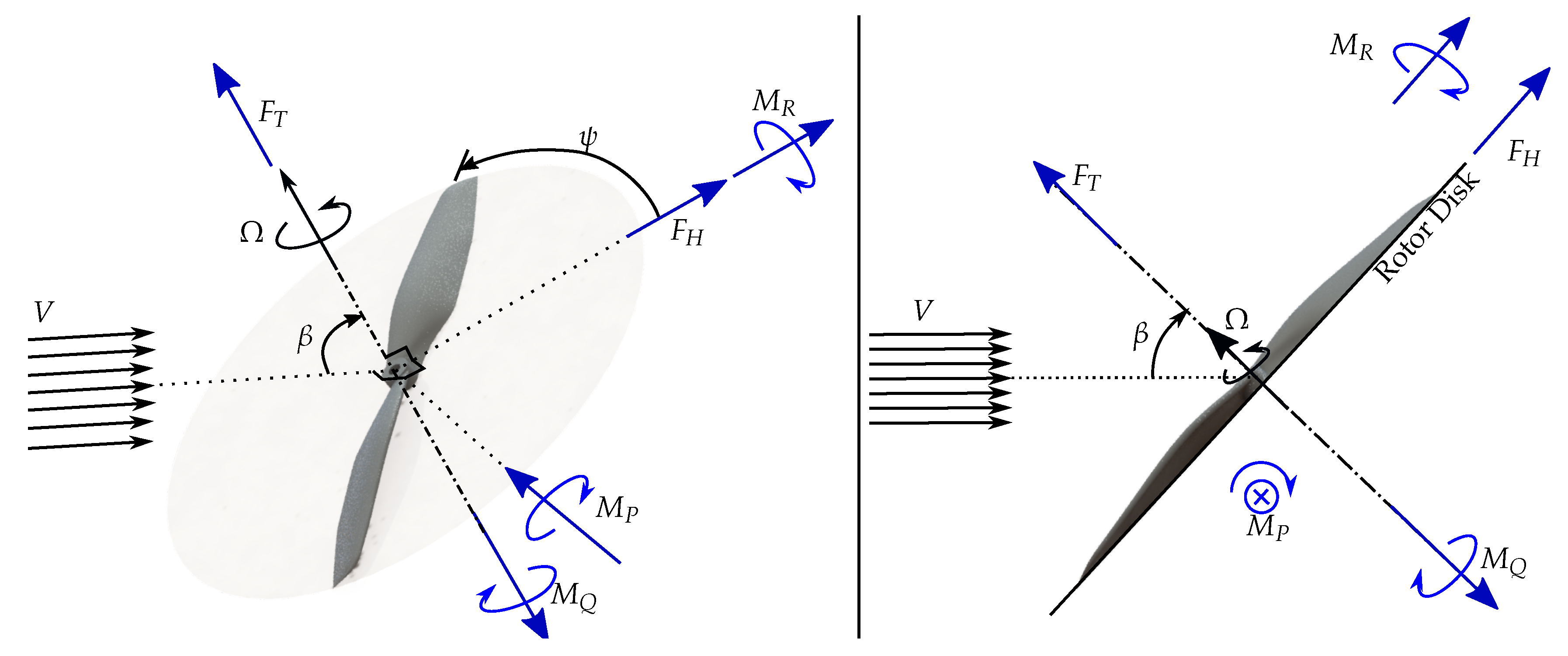
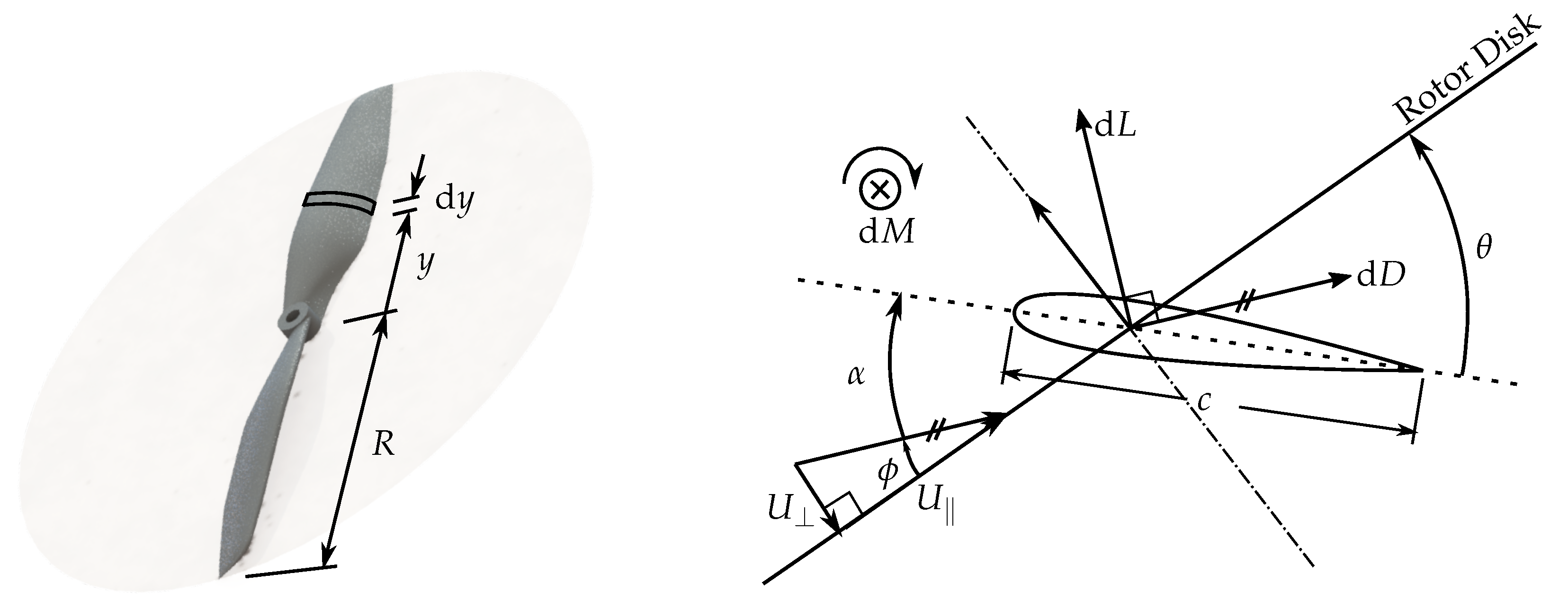
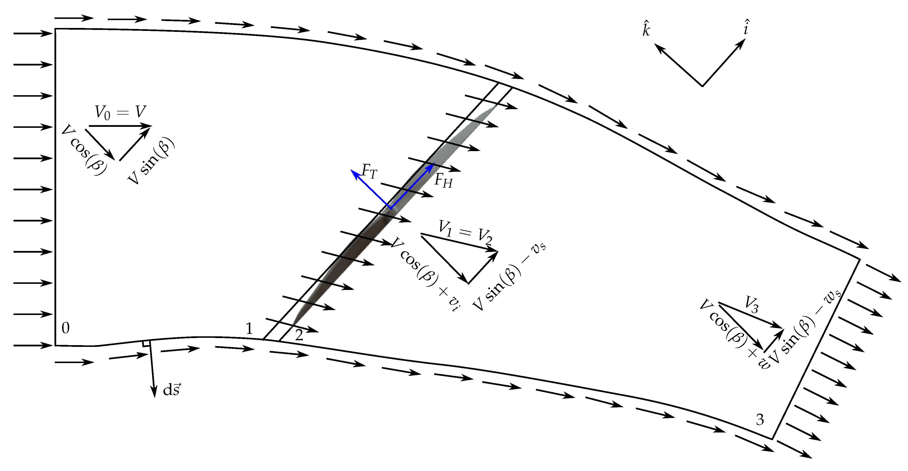
2. First-Principles Derivation
2.1. Thrust
2.2. H-Force
2.3. Rotor Torque
2.4. Rolling Moment
2.5. Pitching Moment
2.6. Induced Inflow
2.7. Summary
2.8. Check if the Assumption is Small is Violated
3. Inferring Parameters from Labelled Data (Supervised Learning)
3.1. Algorithm
3.2. Experimental Assessment
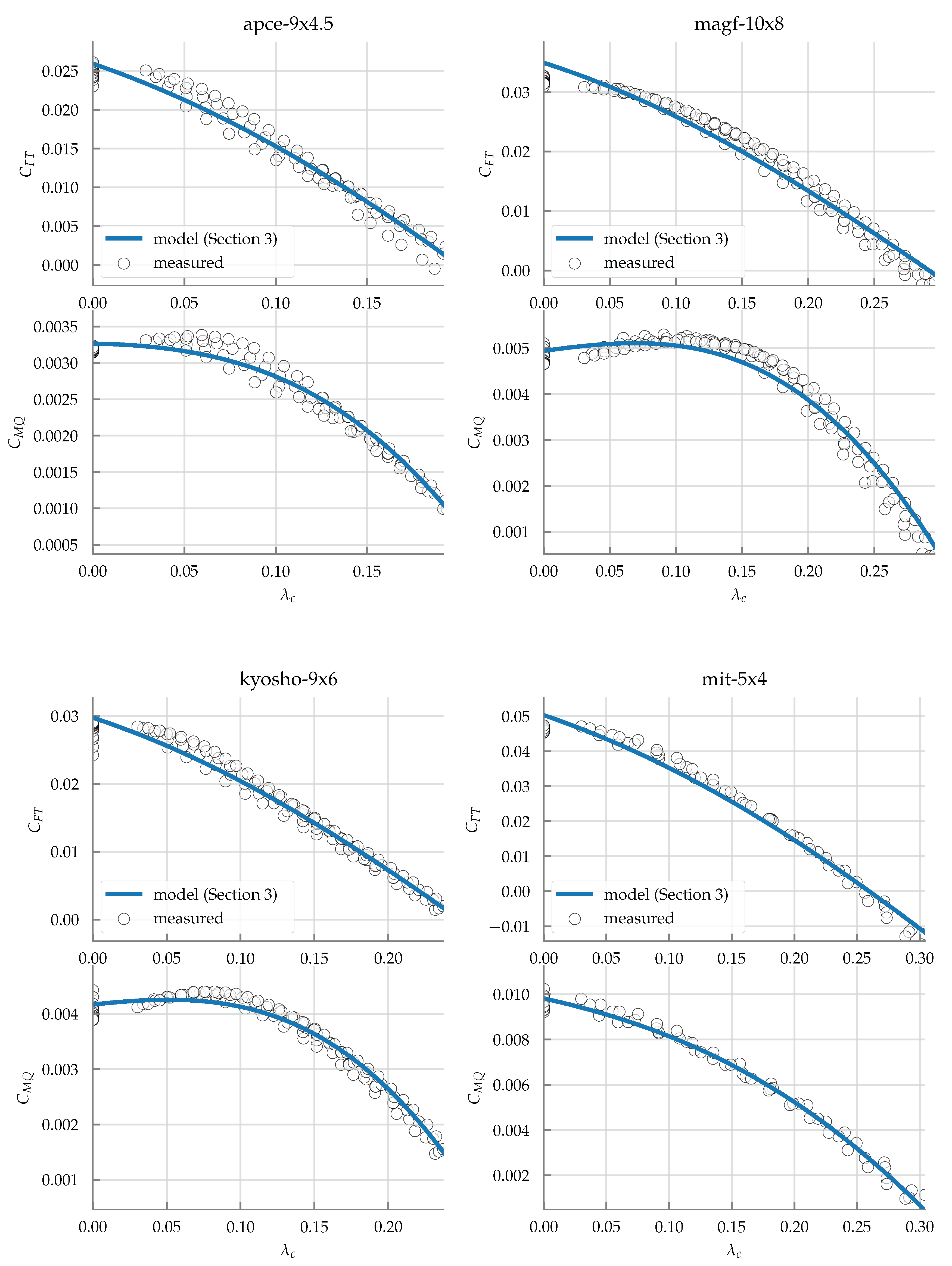
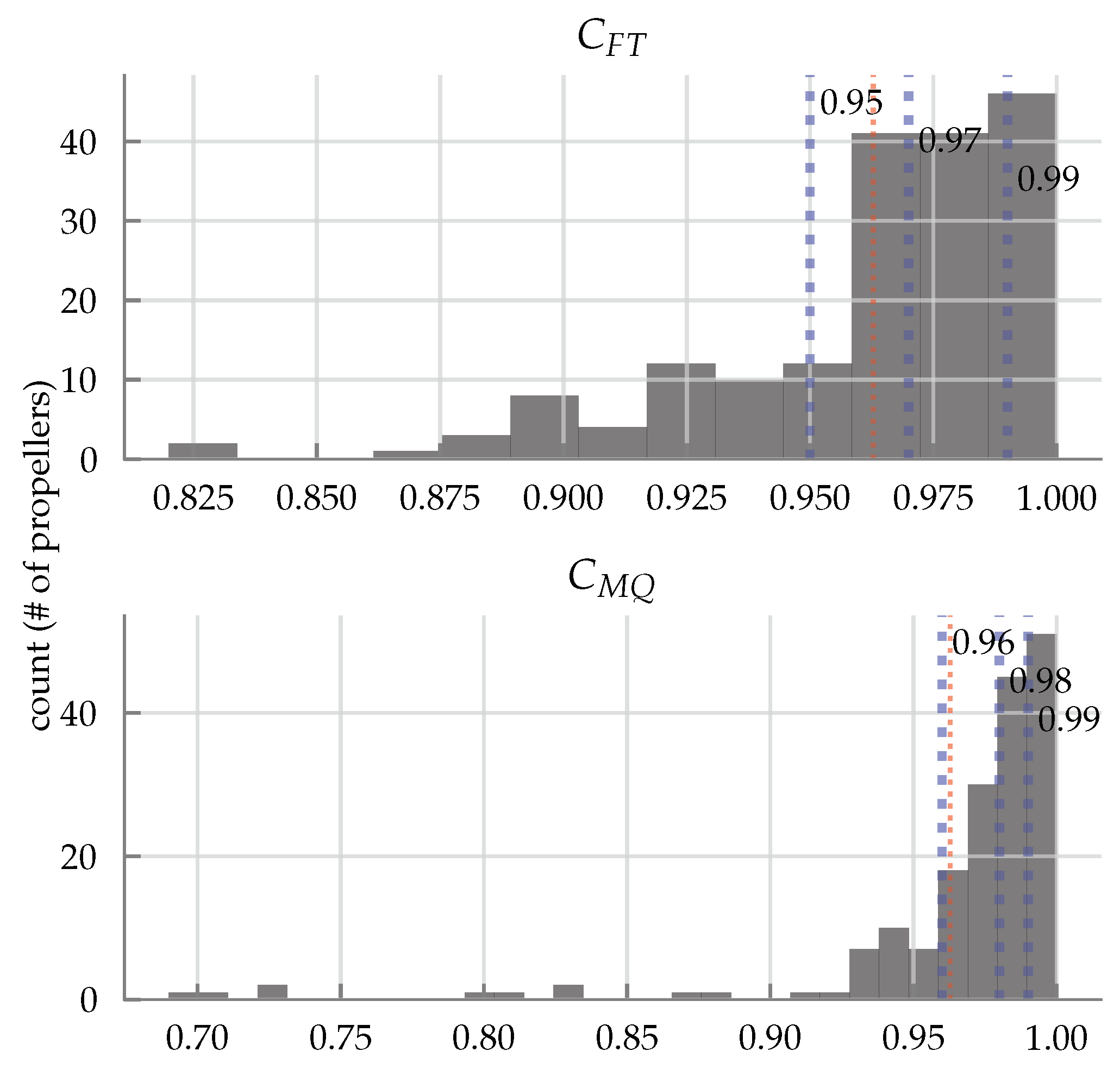
3.2.1. Oblique Flow Results
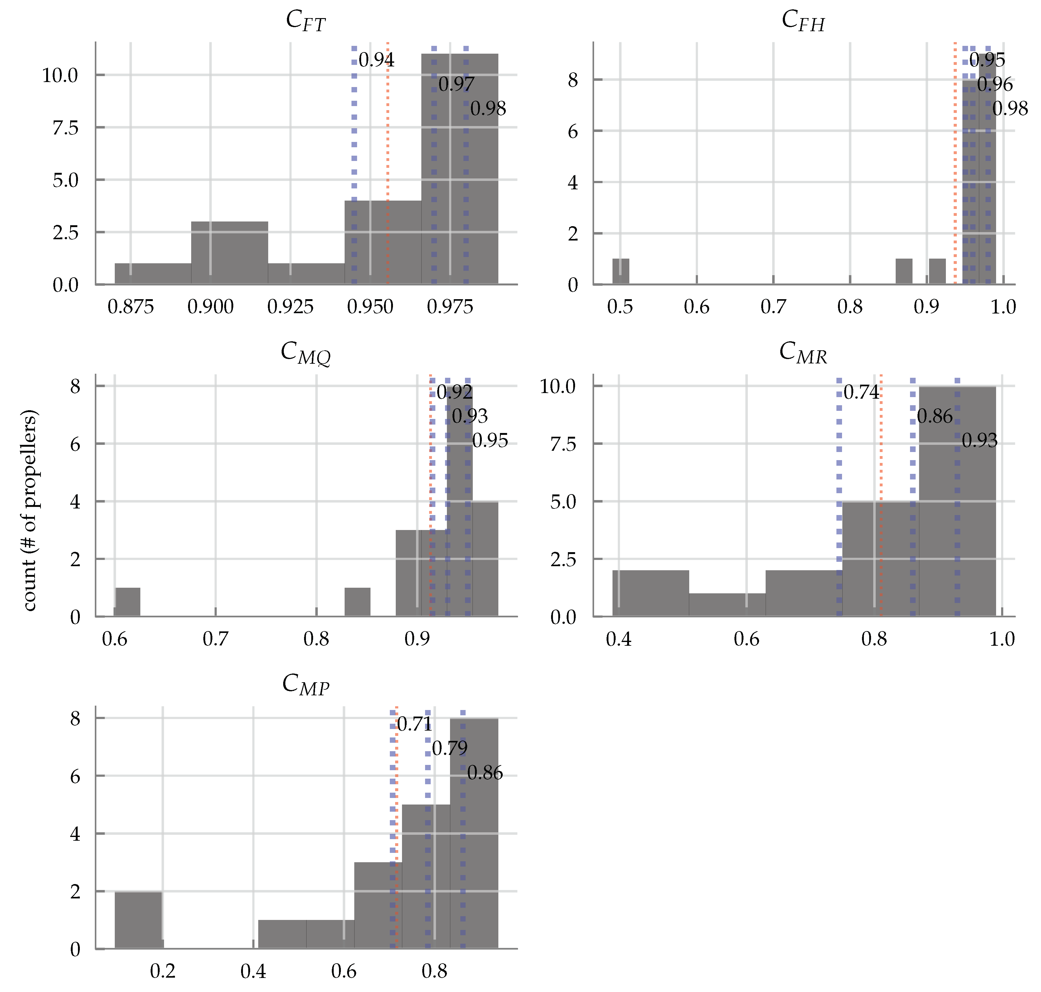
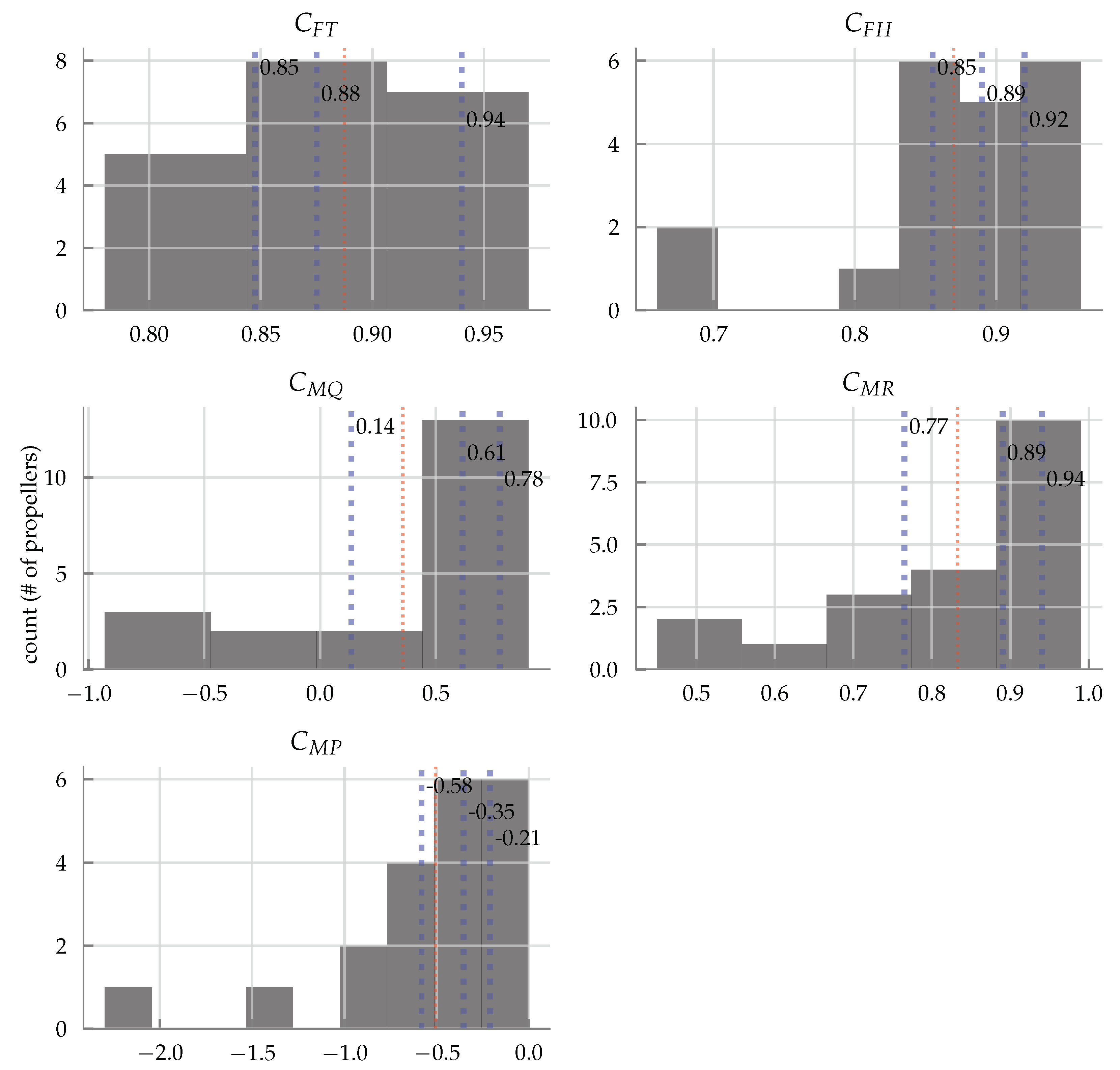
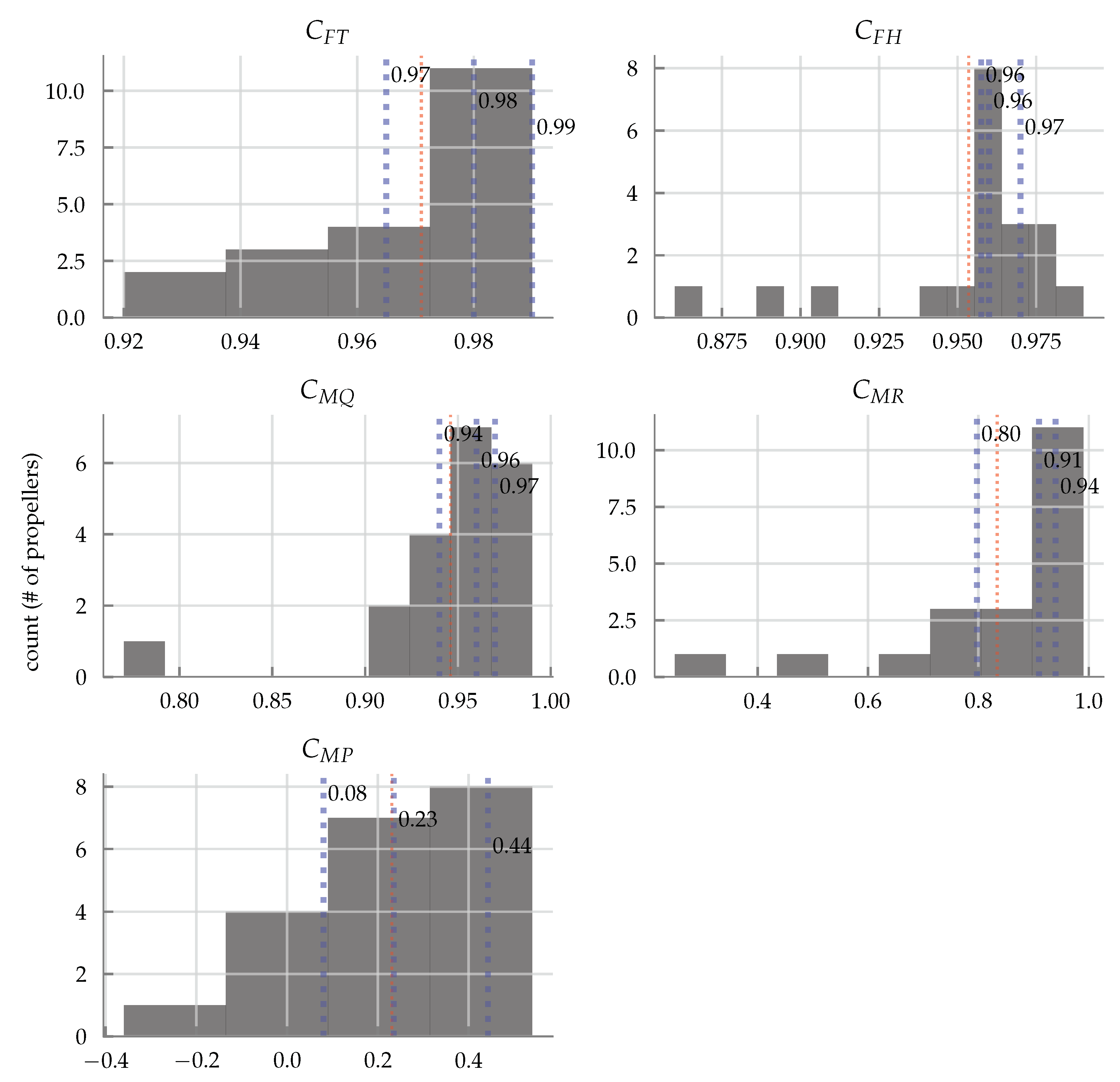
- From the histograms in Figure 9, we can see that the models perform well, especially for the forces , and the rotor torque which have median values above 0.93 (an of 1 corresponds to perfect fit). The rolling and pitching moments have slightly reduced accuracy, with median of 0.86 and 0.79, respectively. However, the metric tends to underestimate the model performance when the data has small values [76], as is the case for the moment coefficients. The values found in Appendix A, or the plots in Supplementary Dataset S1, indeed shows that the model performance is still reasonable for the propellers that have poorer values.
- From the fitted parameter values in Appendix A, we can see that the parameters are in a consistent range of values for both datasets. Occasionally the fitted value exceeds (the theoretical value for a flat plate [70]), which can be expected for non-symmetric airfoils with positive camber [70]. Furthermore, the pitching moment constants , are consistently large in magnitude. From thin airfoil theory, this could again be expected for airfoils with very large positive camber [70]; however, there could be some unmodelled phenomena, possibly due to blade flapping [34], or an artefact of the assumptions made to derive the map (73), and could be a subject for future investigation.
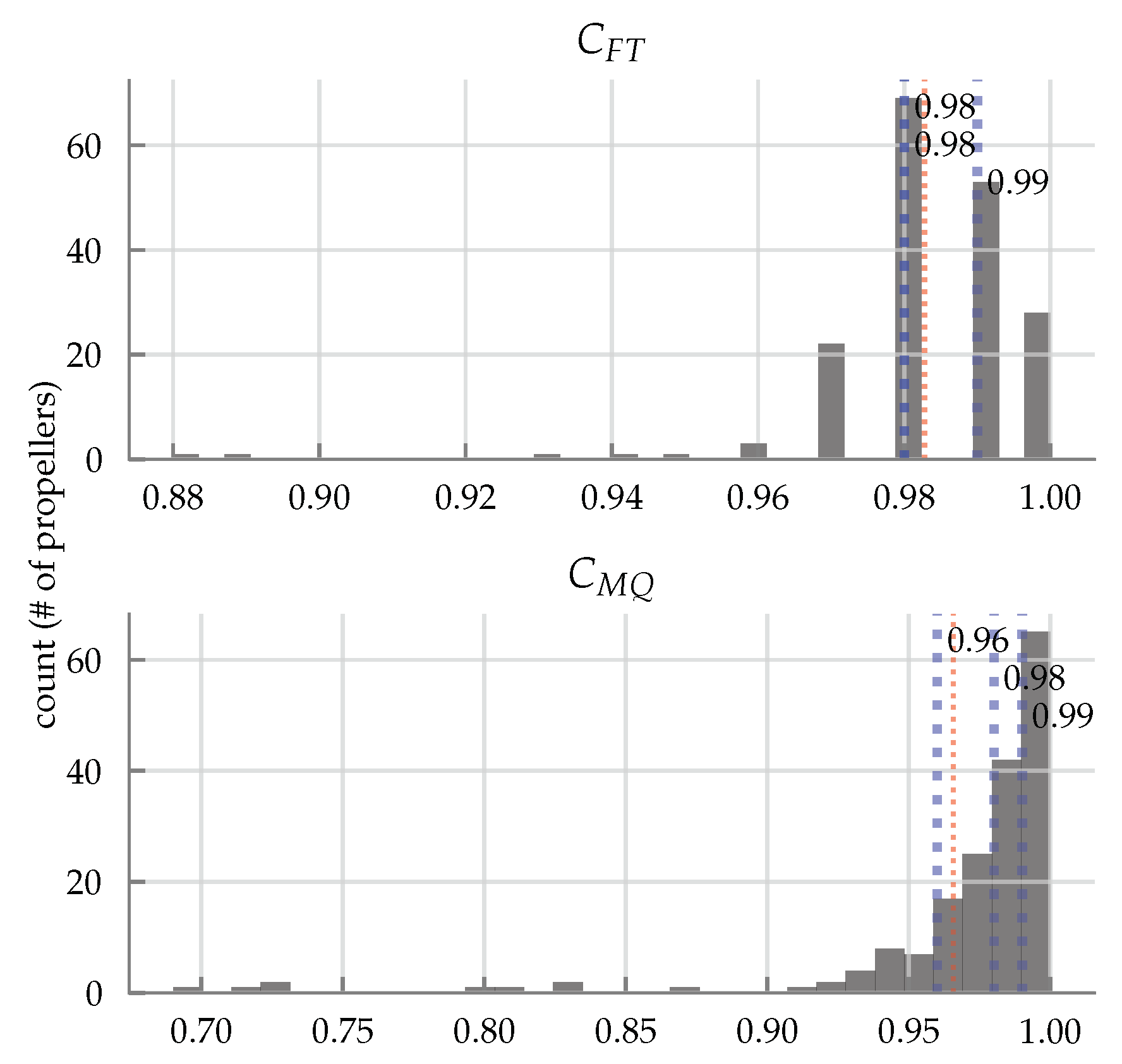
3.2.2. Axial flow Results
4. Inferring Parameters a-priori, without Labelled Data
4.1. Parameter Prediction
4.2. Experimental Assessment
4.2.1. Oblique Flow Results
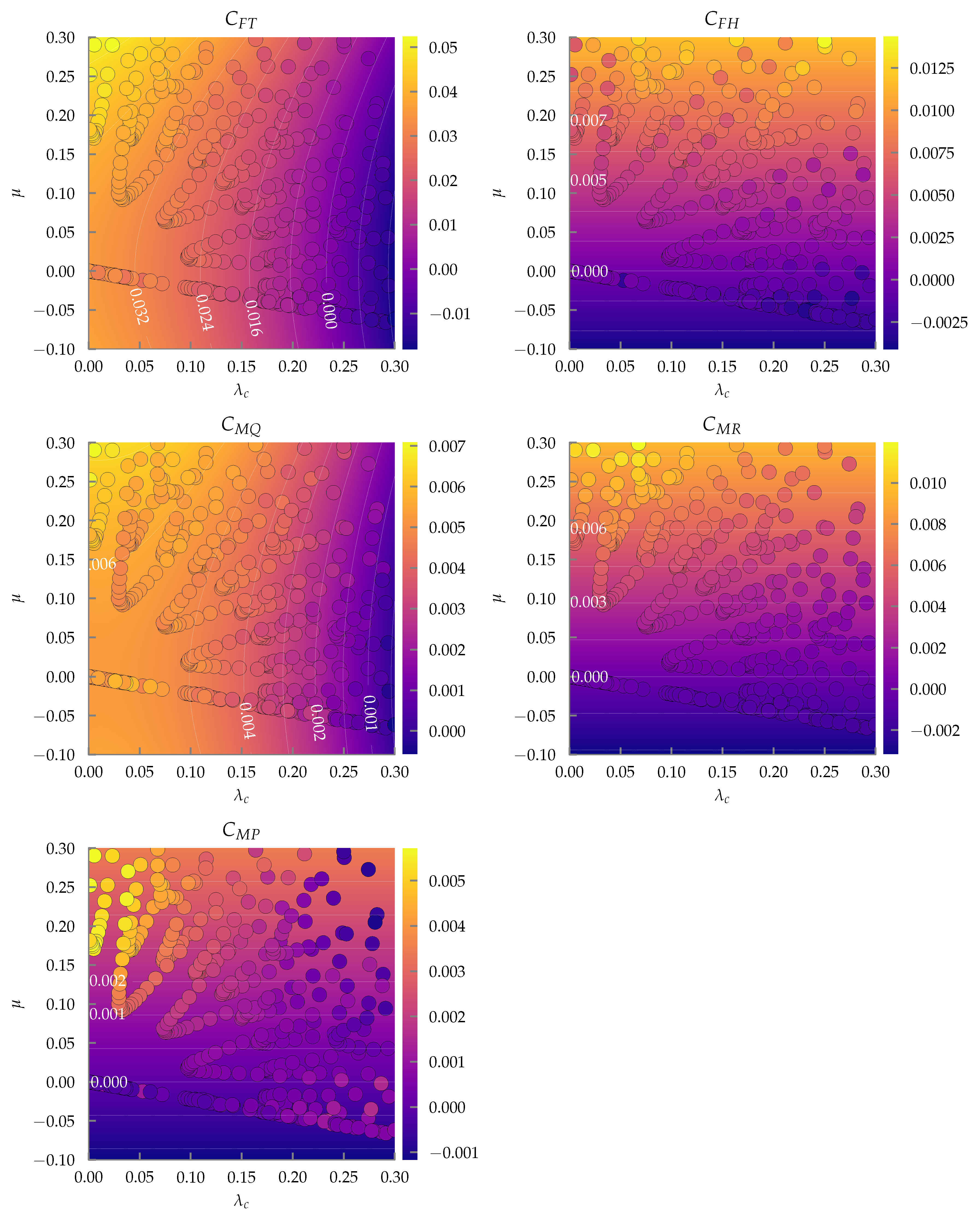
- The thrust, H-force, and rolling moments have (surprisingly) high accuracy, with median values above 0.88.
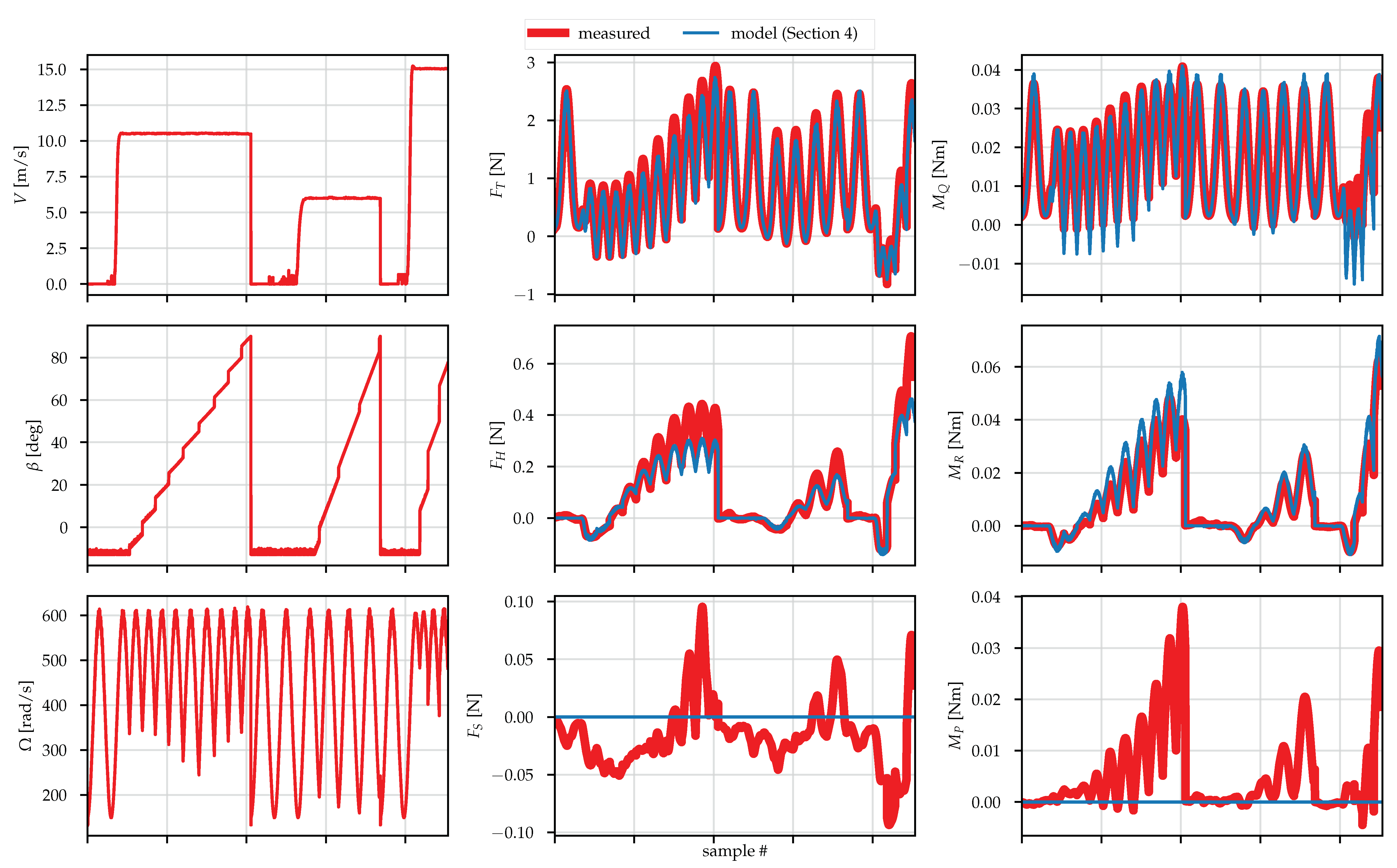
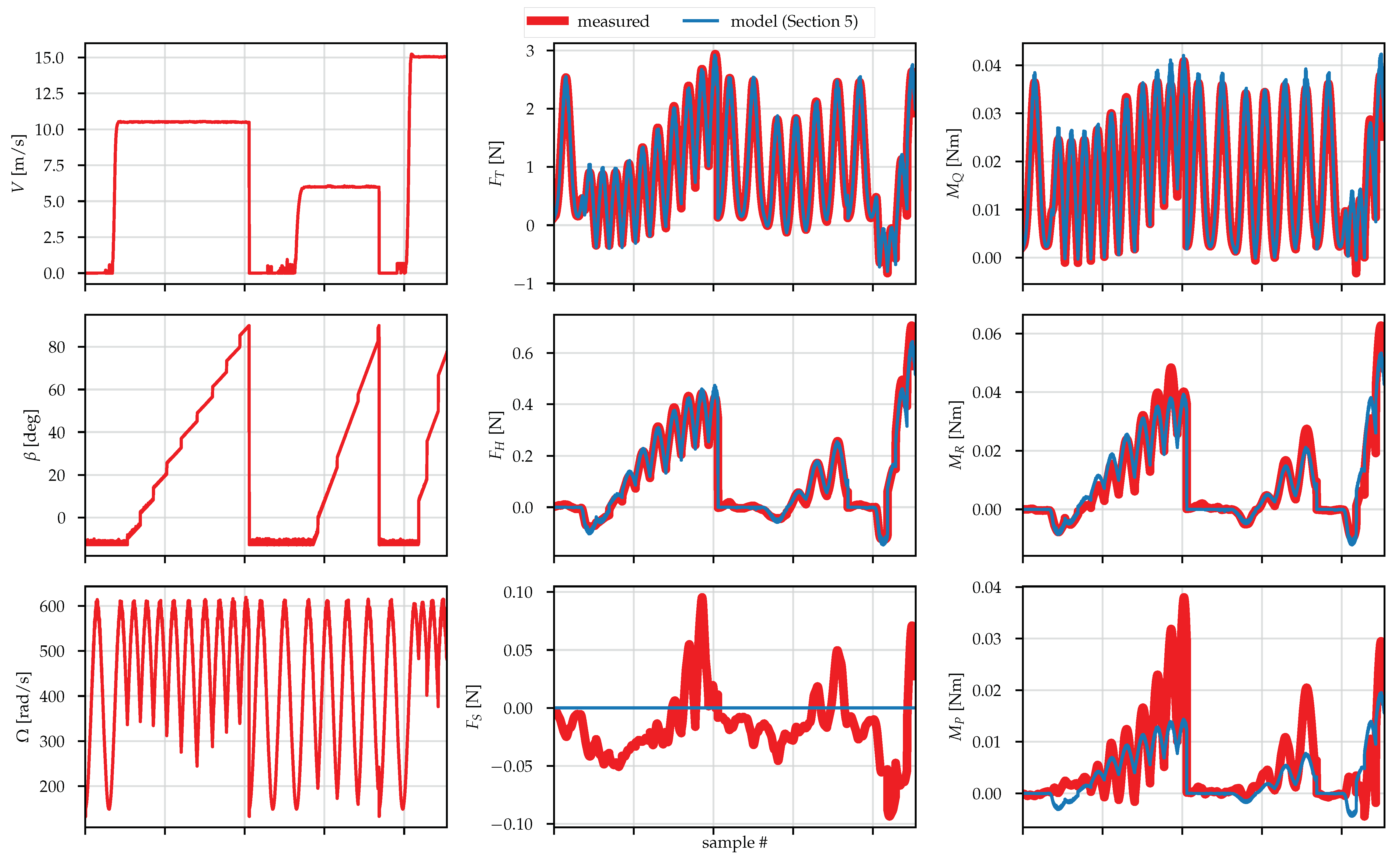
- The rotor torque (median of 0.61) has reduced accuracy for few of the propellers, such as the apcsf, most likely due to severity in the mismatch of the assumed chord model (23). However, typically most of the error for the rotor torque comes at the high ratios, as seen in Figure 12 and Figure 13: in Figure 12, the mismatch in torque occurs when the rotor is producing negative thrust, that is near 0.3 in Figure 13. Thus for small enough operating conditions in , this approach may prove feasible for predicting the rotor torque as well. The pitching moments also have reduced accuracy (median of ), as expected as assuming symmetric airfoils results in the predicted pitching moments to be identically equal to zero, which evidently is not the case.
4.2.2. Axial Flow Results
5. Second-Order Lumped Parameter Models
5.1. Models
5.2. Experimental Assessment
5.2.1. Oblique Flow Results
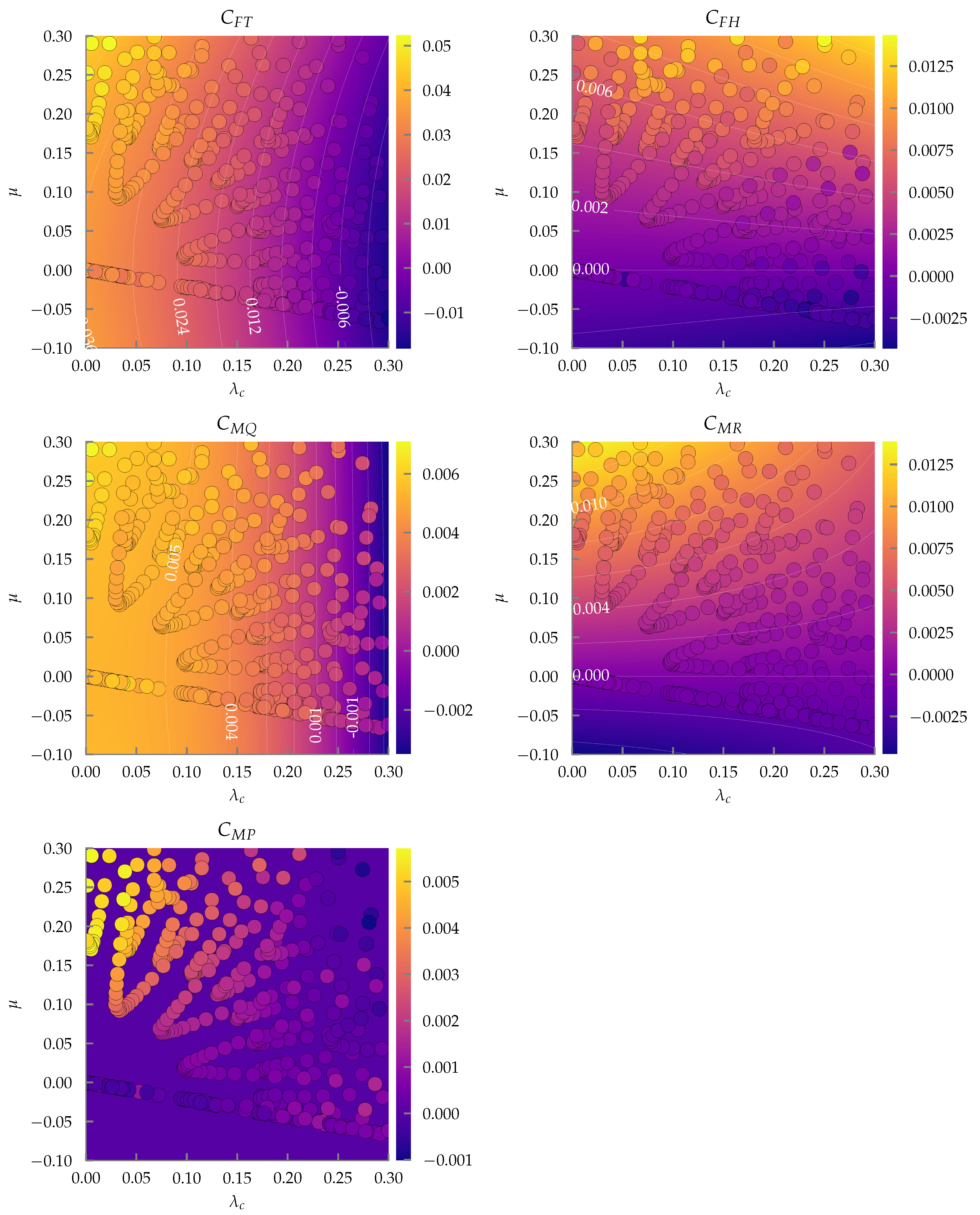
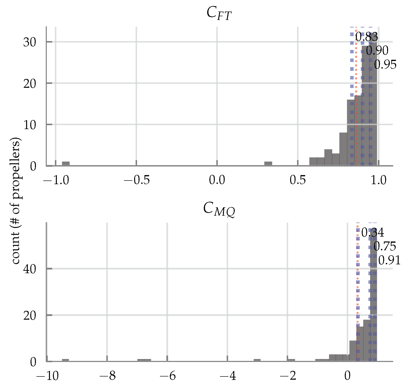
- The models for thrust, H-force, rotor torque, and rolling moments all perform very well, even over the entirety of the tested domain (, ), with median values above 0.91. However, the model for the pitching moment does not, which implies that the domain over which the second-order Taylor expansion for the pitching moment is valid is far smaller than the rest of the models, as can be seen in Figure 17.
- From the parameter values in Table A5 in Appendix A, the parameters and , so these may potentially be ignored in a practical implementation.
5.2.2. Axial Flow Results
6. Conclusion and Future Work
Supplementary Materials
Author Contributions
Funding
Acknowledgments
Conflicts of Interest
Appendix A. Tables of Experimental Results

| Name | |||||||||||||||||||
|---|---|---|---|---|---|---|---|---|---|---|---|---|---|---|---|---|---|---|---|
| ance-12x6 | 0.72 | 6.5 | 0.053 | 3.3 | −2.8 | 18 | 0.15 | 0.17 | 8.4e-3 | 0.99 | 0.91 | 0.97 | 0.91 | 0.85 | 0.033 | 0.056 | 0.050 | 0.077 | 0.072 |
| ance-9x5 | 0.86 | 6.4 | 0.078 | 3.4 | −1.9 | 13 | 0.12 | 0.16 | 6.5e-3 | 0.98 | 0.96 | 0.93 | 0.92 | 0.86 | 0.026 | 0.038 | 0.044 | 0.063 | 0.074 |
| apce-10x7 | 0.75 | 6.6 | 0.12 | 2.8 | −2.4 | 12 | 0.12 | 0.21 | 5.7e-3 | 0.95 | 0.99 | 0.92 | 0.98 | 0.71 | 0.038 | 0.024 | 0.032 | 0.034 | 0.12 |
| apce-12x6 | 0.92 | 8.3 | 0.082 | 4.8 | −2.5 | 24 | 0.10 | 0.14 | 5.7e-3 | 0.99 | 0.99 | 0.96 | 0.90 | 0.84 | 0.030 | 0.023 | 0.043 | 0.066 | 0.080 |
| apce-6x4 | 0.27 | 8.2 | 0.14 | 2.7 | −9.8 | 15 | 0.10 | 0.27 | 2.4e-3 | 0.93 | 0.98 | 0.93 | 0.91 | 0.11 | 0.039 | 0.029 | 0.038 | 0.068 | 0.14 |
| apce-8x6 | 0.79 | 8.3 | 0.16 | 3.5 | −7.8 | 22 | 0.12 | 0.23 | 4.0e-3 | 0.97 | 0.97 | 0.93 | 0.96 | 0.44 | 0.038 | 0.038 | 0.045 | 0.048 | 0.11 |
| apce-8x8 | 0.26 | 10 | 0.16 | 4.3 | 7.2 | 3.2 | 0.16 | 0.39 | 2.4e-3 | 0.91 | 0.97 | 0.89 | 0.99 | 0.094 | 0.055 | 0.035 | 0.055 | 0.028 | 0.18 |
| apcsf-10x4.7 | 0.94 | 6.2 | 0.055 | 3.9 | −0.97 | 18 | 0.13 | 0.13 | 9.7e-3 | 0.97 | 0.95 | 0.94 | 0.70 | 0.92 | 0.030 | 0.044 | 0.031 | 0.11 | 0.063 |
| apcsf-8x3.5 | 0.96 | 7.0 | 0.058 | 4.4 | −1.2 | 16 | 0.10 | 0.13 | 6.6e-3 | 0.99 | 0.96 | 0.96 | 0.82 | 0.88 | 0.022 | 0.042 | 0.036 | 0.083 | 0.080 |
| ef4b-10x6 | 0.75 | 6.3 | 0.065 | 4.3 | −1.4 | 26 | 0.12 | 0.13 | 6.8e-3 | 0.97 | 0.98 | 0.92 | 0.42 | 0.94 | 0.036 | 0.034 | 0.056 | 0.18 | 0.050 |
| grc-10x4 | 0.45 | 6.7 | 0.051 | 5.0 | −2.4 | 27 | 0.17 | 0.097 | 7.1e-3 | 0.98 | 0.49 | 0.94 | 0.39 | 0.77 | 0.038 | 0.12 | 0.057 | 0.11 | 0.079 |
| hqp-7x4.5 | 0.91 | 7.2 | 0.17 | 3.0 | −5.9 | 22 | 0.12 | 0.17 | 4.6e-3 | 0.97 | 0.98 | 0.84 | 0.97 | 0.80 | 0.037 | 0.036 | 0.064 | 0.041 | 0.074 |
| hqp-8x4.5 | 0.87 | 6.3 | 0.13 | 4.5 | −0.30 | 8.3 | 0.14 | 0.16 | 5.9e-3 | 0.95 | 0.95 | 0.92 | 0.96 | 0.60 | 0.045 | 0.057 | 0.041 | 0.048 | 0.16 |
| ma3b-10x5 | 0.12 | 5.8 | 0.079 | 3.8 | −6.4 | 28 | 0.20 | 0.15 | 7.0e-3 | 0.96 | 0.88 | 0.95 | 0.54 | 0.83 | 0.052 | 0.074 | 0.057 | 0.15 | 0.061 |
| ma3b-8x6 | 0.052 | 4.2 | 0.080 | 2.0 | −9.8 | 25 | 0.21 | 0.24 | 6.5e-3 | 0.91 | 0.96 | 0.93 | 0.73 | 0.72 | 0.065 | 0.045 | 0.047 | 0.14 | 0.077 |
| mae-12x6 | 0.84 | 7.7 | 0.17 | 4.8 | −5.3 | 22 | 0.17 | 0.14 | 6.8e-3 | 0.95 | 0.96 | 0.90 | 0.75 | 0.70 | 0.052 | 0.049 | 0.051 | 0.11 | 0.068 |
| magf-8x7 | 0.011 | 3.7 | 8.7e-3 | 2.4 | −9.2 | 14 | 0.22 | 0.33 | 5.7e-3 | 0.87 | 0.97 | 0.90 | 0.82 | 0.73 | 0.075 | 0.040 | 0.054 | 0.11 | 0.069 |
| mamr-10x4.5 | 0.87 | 6.8 | 0.066 | 4.6 | −0.34 | 13 | 0.10 | 0.12 | 9.1e-3 | 0.99 | 0.98 | 0.98 | 0.80 | 0.87 | 0.029 | 0.027 | 0.035 | 0.10 | 0.079 |
| mamr-8x4.5 | 0.97 | 6.7 | 0.087 | 4.0 | −1.7 | 15 | 0.11 | 0.15 | 7.0e-3 | 0.98 | 0.96 | 0.95 | 0.92 | 0.90 | 0.030 | 0.041 | 0.041 | 0.065 | 0.066 |
| gre-9x5 | 0.51 | 4.6 | 0.047 | 2.7 | −4.3 | 30 | 0.16 | 0.15 | 7.6e-3 | 0.90 | 0.95 | 0.60 | 0.82 | 0.76 | 0.061 | 0.041 | 0.070 | 0.069 | 0.12 |
| Name | |||||||||||
|---|---|---|---|---|---|---|---|---|---|---|---|
| ance-8.5x6 | 8.0e-3 | 8.0 | 0.078 | 1.5 | 0.25 | 0.27 | 4.7e-3 | 0.97 | 0.97 | 0.048 | 0.048 |
| ance-8.5x7 | 5.5e-3 | 9.8 | 0.085 | 2.3 | 0.24 | 0.29 | 3.8e-3 | 0.96 | 0.97 | 0.062 | 0.044 |
| apc29ff-9x4 | 0.38 | 8.2 | 0.074 | 2.9 | 0.29 | 0.16 | 6.2e-3 | 0.98 | 0.99 | 0.042 | 0.026 |
| apc29ff-9x5 | 0.013 | 9.9 | 0.082 | 2.0 | 0.30 | 0.23 | 4.6e-3 | 0.97 | 0.97 | 0.056 | 0.049 |
| apccf-7.4x8.25 | 0.16 | 8.2 | 0.22 | 1.7 | 0.32 | 0.37 | 4.0e-3 | 0.93 | 0.98 | 0.072 | 0.037 |
| apccf-7.8x6 | 7.4e-3 | 9.6 | 0.14 | 2.8 | 0.29 | 0.30 | 3.3e-3 | 0.94 | 0.98 | 0.072 | 0.039 |
| apccf-7.8x7 | 3.1e-3 | 9.8 | 0.18 | 3.7 | 0.23 | 0.35 | 2.5e-3 | 0.91 | 0.98 | 0.083 | 0.037 |
| apce-10x5 | 0.014 | 9.4 | 0.068 | 1.2 | 0.20 | 0.21 | 5.3e-3 | 0.98 | 0.97 | 0.044 | 0.051 |
| apce-10x7 | 0.017 | 9.9 | 0.092 | 1.9 | 0.16 | 0.27 | 4.0e-3 | 0.95 | 0.97 | 0.062 | 0.047 |
| apce-11x10 | 0.021 | 9.4 | 0.049 | 3.6 | 0.29 | 0.35 | 4.0e-3 | 0.88 | 0.95 | 0.10 | 0.056 |
| apce-11x5.5 | 0.21 | 4.9 | 0.031 | 1.3 | 0.32 | 0.17 | 0.013 | 0.97 | 0.96 | 0.050 | 0.058 |
| apce-11x7 | 3.1e-3 | 8.8 | 0.058 | 1.2 | 0.36 | 0.25 | 6.9e-3 | 0.96 | 0.96 | 0.058 | 0.062 |
| apce-11x8 | 0.023 | 7.0 | 0.055 | 1.3 | 0.25 | 0.27 | 6.7e-3 | 0.94 | 0.96 | 0.071 | 0.061 |
| apce-11x8.5 | 7.3e-3 | 9.5 | 0.084 | 2.2 | 0.24 | 0.29 | 4.6e-3 | 0.93 | 0.96 | 0.081 | 0.064 |
| apce-14x12 | 0.012 | 9.9 | 0.078 | 3.6 | 0.21 | 0.32 | 4.2e-3 | 0.87 | 0.96 | 0.11 | 0.059 |
| apce-17x12 | 0.0 | 9.8 | 0.053 | 2.8 | 0.31 | 0.29 | 6.6e-3 | 0.89 | 0.95 | 0.10 | 0.065 |
| apce-19x12 | 5.8e-3 | 5.7 | 0.040 | 0.91 | 0.32 | 0.25 | 0.015 | 0.94 | 0.93 | 0.072 | 0.073 |
| apce-8x4 | 0.49 | 7.4 | 0.080 | 2.7 | 0.13 | 0.18 | 4.5e-3 | 0.99 | 0.98 | 0.033 | 0.037 |
| apce-8x6 | 5.9e-3 | 8.2 | 0.091 | 2.5 | 0.36 | 0.32 | 4.5e-3 | 0.94 | 0.97 | 0.077 | 0.049 |
| apce-8x8 | 0.011 | 6.1 | 0.11 | 2.4 | 0.19 | 0.41 | 4.0e-3 | 0.90 | 0.97 | 0.090 | 0.043 |
| apce-9x4.5 | 0.35 | 8.0 | 0.069 | 1.8 | 0.17 | 0.17 | 5.8e-3 | 0.98 | 0.98 | 0.046 | 0.044 |
| apce-9x6 | 0.017 | 8.1 | 0.080 | 1.3 | 0.12 | 0.26 | 4.8e-3 | 0.98 | 0.98 | 0.042 | 0.041 |
| apce-9x7.5 | 4.6e-4 | 4.6 | 0.061 | 1.4 | 0.16 | 0.33 | 7.2e-3 | 0.93 | 0.96 | 0.080 | 0.051 |
| apce-9x9 | 0.027 | 9.4 | 0.11 | 3.4 | 0.33 | 0.38 | 3.9e-3 | 0.92 | 0.97 | 0.079 | 0.044 |
| apcff-4.2x4 | 3.9e-3 | 8.2 | 0.22 | 4.0 | 0.22 | 0.34 | 1.9e-3 | 0.96 | 0.98 | 0.056 | 0.032 |
| apcff-9x4 | 0.33 | 8.2 | 0.089 | 3.0 | 0.11 | 0.16 | 5.4e-3 | 0.98 | 0.99 | 0.044 | 0.029 |
| apcsf-10x4.7 | 0.81 | 6.5 | 0.050 | 3.3 | 0.20 | 0.14 | 0.010 | 0.99 | 0.97 | 0.031 | 0.042 |
| apcsf-10x7 | 0.77 | 6.4 | 0.064 | 2.6 | 0.26 | 0.20 | 9.9e-3 | 0.98 | 0.96 | 0.037 | 0.053 |
| apcsf-11x3.8 | 0.59 | 6.3 | 0.029 | 4.5 | 0.37 | 0.092 | 0.017 | 0.99 | 0.98 | 0.030 | 0.040 |
| apcsf-11x4.7 | 0.75 | 5.8 | 0.040 | 3.6 | 0.13 | 0.12 | 0.013 | 0.98 | 0.97 | 0.034 | 0.047 |
| apcsf-11x7 | 1.0 | 8.0 | 0.083 | 3.0 | 0.21 | 0.19 | 8.7e-3 | 0.99 | 0.98 | 0.032 | 0.042 |
| apcsf-8x3.8 | 0.65 | 5.5 | 0.056 | 3.3 | 0.22 | 0.13 | 8.5e-3 | 0.99 | 0.98 | 0.031 | 0.036 |
| apcsf-8x6 | 0.66 | 8.7 | 0.11 | 2.9 | 0.27 | 0.27 | 4.8e-3 | 0.98 | 0.97 | 0.041 | 0.042 |
| apcsf-9x3.8 | 0.65 | 5.7 | 0.045 | 3.6 | 0.20 | 0.11 | 0.010 | 0.98 | 0.97 | 0.032 | 0.041 |
| apcsf-9x4.7 | 0.66 | 6.7 | 0.041 | 4.2 | 0.40 | 0.13 | 0.012 | 0.99 | 0.99 | 0.021 | 0.024 |
| apcsf-9x6 | 0.64 | 6.5 | 0.067 | 2.2 | 0.32 | 0.23 | 8.9e-3 | 0.98 | 0.95 | 0.041 | 0.057 |
| apcsf-9x7.5 | 0.69 | 7.2 | 0.097 | 3.1 | 0.24 | 0.28 | 6.5e-3 | 0.97 | 0.94 | 0.045 | 0.057 |
| apcsp-10x10 | 9.5e-3 | 9.0 | 0.23 | 3.9 | 0.34 | 0.37 | 4.0e-3 | 0.93 | 0.99 | 0.074 | 0.029 |
| apcsp-10x3 | 0.35 | 9.7 | 0.062 | 4.2 | 0.40 | 0.13 | 6.8e-3 | 0.97 | 0.99 | 0.049 | 0.030 |
| apcsp-10x4 | 0.38 | 7.7 | 0.065 | 2.4 | 0.27 | 0.15 | 7.7e-3 | 0.98 | 0.99 | 0.036 | 0.024 |
| apcsp-10x5 | 0.042 | 9.5 | 0.075 | 1.7 | 0.27 | 0.22 | 5.8e-3 | 0.98 | 0.98 | 0.042 | 0.033 |
| apcsp-10x6 | 8.1e-3 | 8.5 | 0.092 | 1.3 | 0.14 | 0.26 | 5.0e-3 | 0.96 | 0.97 | 0.058 | 0.046 |
| apcsp-10x7 | 0.015 | 9.5 | 0.11 | 2.0 | 0.28 | 0.27 | 4.9e-3 | 0.94 | 0.96 | 0.071 | 0.052 |
| apcsp-10x8 | 6.7e-3 | 9.9 | 0.12 | 2.6 | 0.19 | 0.31 | 3.7e-3 | 0.91 | 0.95 | 0.089 | 0.059 |
| apcsp-10x9 | 0.011 | 8.3 | 0.14 | 2.8 | 0.24 | 0.35 | 4.2e-3 | 0.89 | 0.96 | 0.095 | 0.048 |
| apcsp-11x3 | 0.49 | 8.4 | 0.080 | 3.8 | 0.18 | 0.11 | 6.4e-3 | 0.98 | 0.99 | 0.042 | 0.027 |
| apcsp-11x4 | 0.54 | 9.9 | 0.10 | 4.3 | 0.25 | 0.14 | 5.7e-3 | 0.97 | 0.99 | 0.051 | 0.028 |
| apcsp-11x5 | 0.21 | 8.7 | 0.067 | 1.7 | 0.38 | 0.19 | 8.2e-3 | 0.97 | 0.98 | 0.052 | 0.042 |
| apcsp-11x6 | 0.026 | 8.7 | 0.084 | 1.2 | 0.32 | 0.24 | 7.0e-3 | 0.96 | 0.98 | 0.057 | 0.045 |
| apcsp-11x7 | 0.033 | 7.6 | 0.091 | 1.3 | 0.18 | 0.27 | 6.1e-3 | 0.95 | 0.97 | 0.063 | 0.045 |
| apcsp-11x8 | 2.0e-3 | 9.5 | 0.11 | 1.5 | 0.30 | 0.30 | 5.4e-3 | 0.94 | 0.96 | 0.068 | 0.049 |
| apcsp-11x9 | 0.014 | 9.7 | 0.11 | 2.4 | 0.18 | 0.34 | 3.8e-3 | 0.90 | 0.93 | 0.087 | 0.062 |
| apcsp-14x13 | 5.6e-3 | 8.1 | 0.081 | 2.7 | 0.37 | 0.36 | 6.9e-3 | 0.89 | 0.94 | 0.096 | 0.060 |
| apcsp-4.2x2 | 0.29 | 6.0 | 0.083 | 3.9 | 0.17 | 0.16 | 3.2e-3 | 0.98 | 0.99 | 0.038 | 0.024 |
| apcsp-7x6 | 5.8e-4 | 5.1 | 0.13 | 1.9 | 0.33 | 0.32 | 4.5e-3 | 0.94 | 0.98 | 0.067 | 0.033 |
| apcsp-7x9 | 0.016 | 7.4 | 0.18 | 3.4 | 0.36 | 0.50 | 2.4e-3 | 0.82 | 0.94 | 0.11 | 0.054 |
| apcsp-8x10 | 0.014 | 6.8 | 0.46 | 3.2 | 0.11 | 0.47 | 2.4e-3 | 0.89 | 0.97 | 0.074 | 0.036 |
| apcsp-8x4 | 0.010 | 9.9 | 0.11 | 3.0 | 0.21 | 0.21 | 3.3e-3 | 0.98 | 0.99 | 0.041 | 0.030 |
| apcsp-8x5 | 1.6e-3 | 9.6 | 0.15 | 2.7 | 0.33 | 0.25 | 3.6e-3 | 0.97 | 0.99 | 0.046 | 0.027 |
| apcsp-8x6 | 4.2e-3 | 5.6 | 0.13 | 1.5 | 0.23 | 0.29 | 5.0e-3 | 0.95 | 0.99 | 0.063 | 0.031 |
| apcsp-8x7 | 5.2e-4 | 9.6 | 0.18 | 2.7 | 0.36 | 0.32 | 3.4e-3 | 0.89 | 0.96 | 0.098 | 0.054 |
| apcsp-8x8 | 1.9e-3 | 8.3 | 0.26 | 3.0 | 0.20 | 0.39 | 2.5e-3 | 0.88 | 0.96 | 0.093 | 0.046 |
| apcsp-8x9 | 5.3e-3 | 9.3 | 0.47 | 3.8 | 0.22 | 0.46 | 1.9e-3 | 0.83 | 0.94 | 0.090 | 0.046 |
| apcsp-9x10 | 0.028 | 9.8 | 0.25 | 3.0 | 0.23 | 0.41 | 2.6e-3 | 0.92 | 0.93 | 0.076 | 0.057 |
| apcsp-9x6 | 1.5e-3 | 6.2 | 0.078 | 1.4 | 0.24 | 0.27 | 6.5e-3 | 0.95 | 0.97 | 0.060 | 0.043 |
| apcsp-9x7 | 9.4e-3 | 8.9 | 0.11 | 1.9 | 0.20 | 0.30 | 3.9e-3 | 0.94 | 0.95 | 0.076 | 0.058 |
| apcsp-9x8 | 5.7e-3 | 7.9 | 0.20 | 2.7 | 0.11 | 0.33 | 3.3e-3 | 0.92 | 0.98 | 0.086 | 0.041 |
| apcsp-9x9 | 2.8e-3 | 9.6 | 0.23 | 4.4 | 0.39 | 0.38 | 3.2e-3 | 0.92 | 0.98 | 0.073 | 0.036 |
| da4002-5x1.58 | 0.16 | 6.3 | 0.080 | 3.5 | 0.11 | 0.14 | 4.0e-3 | 0.97 | 0.98 | 0.057 | 0.036 |
| da4002-5x2.65 | 9.4e-3 | 7.2 | 0.11 | 3.5 | 0.11 | 0.21 | 3.1e-3 | 0.99 | 0.99 | 0.037 | 0.028 |
| da4002-5x3.75 | 2.3e-3 | 8.8 | 0.15 | 4.5 | 0.13 | 0.29 | 2.3e-3 | 0.98 | 0.99 | 0.045 | 0.023 |
| da4002-5x4.92 | 6.0e-4 | 8.7 | 0.19 | 5.0 | 0.25 | 0.38 | 2.3e-3 | 0.96 | 0.99 | 0.059 | 0.029 |
| da4002-9x2.85 | 1.4e-3 | 9.7 | 0.070 | 2.6 | 0.23 | 0.16 | 5.6e-3 | 0.99 | 0.98 | 0.032 | 0.034 |
| da4002-9x4.76 | 0.039 | 8.5 | 0.087 | 2.3 | 0.11 | 0.22 | 4.9e-3 | 0.99 | 0.99 | 0.030 | 0.030 |
| da4002-9x6.75 | 0.019 | 7.9 | 0.082 | 2.8 | 0.21 | 0.29 | 5.3e-3 | 0.98 | 0.98 | 0.037 | 0.033 |
| da4002-9x8.95 | 0.029 | 8.4 | 0.090 | 3.9 | 0.16 | 0.37 | 4.0e-3 | 0.97 | 0.98 | 0.053 | 0.035 |
| da4022-5x3.75 | 0.31 | 7.3 | 0.074 | 4.9 | 0.38 | 0.23 | 8.3e-3 | 0.89 | 0.73 | 0.093 | 0.13 |
| da4022-9x6.75 | 0.029 | 7.2 | 0.066 | 2.0 | 0.28 | 0.25 | 0.012 | 0.88 | 0.69 | 0.091 | 0.13 |
| da4052-5x1.58 | 0.24 | 6.5 | 0.063 | 5.0 | 0.26 | 0.10 | 4.4e-3 | 0.99 | 0.87 | 0.025 | 0.10 |
| da4052-5x2.65 | 0.38 | 8.4 | 0.090 | 5.0 | 0.23 | 0.15 | 3.3e-3 | 1.0 | 0.94 | 0.016 | 0.067 |
| da4052-5x3.75 | 6.6e-3 | 6.4 | 0.080 | 3.0 | 0.26 | 0.24 | 5.7e-3 | 0.93 | 0.83 | 0.072 | 0.10 |
| da4052-5x4.92 | 0.29 | 6.7 | 0.084 | 4.7 | 0.19 | 0.28 | 3.4e-3 | 0.99 | 0.98 | 0.033 | 0.034 |
| da4052-9x2.85 | 4.7e-3 | 5.1 | 0.051 | 2.1 | 0.14 | 0.13 | 8.3e-3 | 0.99 | 0.94 | 0.028 | 0.068 |
| da4052-9x4.76 | 2.1e-3 | 7.1 | 0.068 | 1.7 | 0.18 | 0.19 | 6.4e-3 | 1.0 | 0.95 | 0.021 | 0.053 |
| da4052-9x6.75 | 0.031 | 6.2 | 0.054 | 2.3 | 0.21 | 0.25 | 8.3e-3 | 0.93 | 0.83 | 0.077 | 0.099 |
| da4052-9x8.95 | 0.24 | 7.6 | 0.059 | 4.4 | 0.29 | 0.31 | 5.3e-3 | 0.97 | 0.98 | 0.049 | 0.038 |
| ef-130x70 | 0.51 | 7.1 | 0.058 | 4.7 | 0.30 | 0.16 | 4.4e-3 | 0.98 | 0.99 | 0.037 | 0.028 |
| grcp-10x6 | 5.0e-3 | 7.1 | 0.091 | 0.94 | 0.12 | 0.23 | 5.5e-3 | 0.98 | 0.98 | 0.042 | 0.034 |
| grcp-10x8 | 0.011 | 9.3 | 0.14 | 2.3 | 0.14 | 0.30 | 3.5e-3 | 0.95 | 0.97 | 0.063 | 0.043 |
| grcp-11x4 | 0.44 | 8.8 | 0.078 | 3.0 | 0.23 | 0.12 | 6.0e-3 | 0.97 | 0.98 | 0.054 | 0.041 |
| grcp-11x6 | 0.15 | 7.6 | 0.084 | 1.4 | 0.13 | 0.18 | 6.0e-3 | 0.97 | 0.98 | 0.053 | 0.044 |
| grcp-11x8 | 0.011 | 8.2 | 0.078 | 1.8 | 0.36 | 0.29 | 6.1e-3 | 0.96 | 0.97 | 0.059 | 0.047 |
| grcp-9x4 | 0.42 | 9.2 | 0.088 | 3.7 | 0.38 | 0.13 | 5.4e-3 | 0.98 | 0.99 | 0.040 | 0.030 |
| grcp-9x6 | 0.020 | 7.9 | 0.11 | 1.4 | 0.19 | 0.24 | 4.7e-3 | 0.97 | 0.99 | 0.050 | 0.033 |
| grcsp-10x6 | 0.70 | 9.6 | 0.095 | 2.1 | 0.32 | 0.22 | 6.0e-3 | 0.98 | 0.98 | 0.040 | 0.041 |
| grcsp-10x8 | 3.4e-3 | 9.3 | 0.13 | 1.8 | 0.18 | 0.34 | 4.2e-3 | 0.96 | 0.98 | 0.060 | 0.038 |
| grcsp-9x5 | 3.4e-3 | 8.8 | 0.059 | 1.8 | 0.18 | 0.20 | 4.7e-3 | 0.99 | 1.0 | 0.026 | 0.016 |
| grcsp-9x6 | 2.3e-3 | 6.3 | 0.077 | 1.4 | 0.25 | 0.31 | 6.7e-3 | 0.97 | 0.99 | 0.048 | 0.027 |
| grsn-10x6 | 0.021 | 8.1 | 0.054 | 1.4 | 0.28 | 0.22 | 7.9e-3 | 0.99 | 0.99 | 0.031 | 0.034 |
| grsn-10x7 | 5.1e-3 | 9.3 | 0.083 | 1.5 | 0.18 | 0.27 | 5.4e-3 | 0.98 | 0.97 | 0.042 | 0.049 |
| grsn-11x10 | 0.013 | 8.6 | 0.12 | 0.94 | 0.23 | 0.31 | 6.6e-3 | 0.98 | 0.98 | 0.045 | 0.042 |
| grsn-11x6 | 0.022 | 9.7 | 0.059 | 1.6 | 0.26 | 0.19 | 7.7e-3 | 0.99 | 0.98 | 0.034 | 0.036 |
| grsn-11x7 | 3.7e-3 | 9.6 | 0.081 | 1.7 | 0.11 | 0.23 | 5.6e-3 | 0.98 | 0.99 | 0.040 | 0.036 |
| grsn-11x8 | 4.9e-3 | 8.3 | 0.080 | 1.2 | 0.10 | 0.25 | 6.5e-3 | 0.98 | 0.97 | 0.040 | 0.049 |
| grsn-9x4 | 0.48 | 9.8 | 0.097 | 3.5 | 0.14 | 0.15 | 5.0e-3 | 0.99 | 0.99 | 0.036 | 0.023 |
| grsn-9x5 | 5.4e-3 | 8.8 | 0.073 | 1.5 | 0.28 | 0.21 | 6.5e-3 | 0.99 | 0.99 | 0.036 | 0.031 |
| grsn-9x6 | 0.016 | 8.7 | 0.080 | 1.4 | 0.28 | 0.25 | 6.3e-3 | 0.98 | 0.98 | 0.041 | 0.036 |
| grsn-9x7 | 6.8e-3 | 9.8 | 0.12 | 1.3 | 0.31 | 0.31 | 5.2e-3 | 0.98 | 0.96 | 0.046 | 0.052 |
| gwsdd-10x6 | 0.63 | 9.8 | 0.075 | 1.9 | 0.23 | 0.16 | 5.6e-3 | 0.99 | 0.99 | 0.030 | 0.032 |
| gwsdd-11x7 | 0.48 | 6.4 | 0.043 | 1.7 | 0.25 | 0.16 | 0.011 | 0.99 | 0.99 | 0.027 | 0.034 |
| gwsdd-2.5x0.8 | 0.20 | 4.6 | 0.053 | 4.9 | 0.12 | 0.092 | 3.6e-3 | 1.0 | 0.71 | 0.019 | 0.076 |
| gwsdd-2.5x1 | 0.30 | 5.2 | 0.052 | 5.0 | 0.16 | 0.098 | 3.6e-3 | 1.0 | 0.94 | 0.016 | 0.060 |
| gwsdd-3x2 | 0.43 | 5.9 | 0.055 | 4.8 | 0.30 | 0.16 | 4.4e-3 | 1.0 | 0.98 | 0.018 | 0.031 |
| gwsdd-3x3 | 0.37 | 3.8 | 0.059 | 3.1 | 0.17 | 0.25 | 5.2e-3 | 0.99 | 1.0 | 0.023 | 0.014 |
| gwsdd-4.5x3 | 0.32 | 4.6 | 0.037 | 3.3 | 0.34 | 0.16 | 7.5e-3 | 0.99 | 0.99 | 0.022 | 0.029 |
| gwsdd-4.5x4 | 0.42 | 4.9 | 0.072 | 2.6 | 0.27 | 0.23 | 5.7e-3 | 1.0 | 0.98 | 0.021 | 0.038 |
| gwsdd-4x2.5 | 0.39 | 5.1 | 0.042 | 4.8 | 0.12 | 0.15 | 5.5e-3 | 1.0 | 0.97 | 0.014 | 0.043 |
| gwsdd-4x4 | 0.38 | 5.6 | 0.089 | 4.0 | 0.34 | 0.26 | 5.0e-3 | 0.99 | 1.0 | 0.031 | 0.016 |
| gwsdd-5x3 | 0.45 | 6.5 | 0.042 | 5.0 | 0.34 | 0.14 | 6.4e-3 | 1.0 | 0.98 | 0.014 | 0.036 |
| gwsdd-5x4.3 | 0.42 | 4.2 | 0.050 | 3.4 | 0.20 | 0.20 | 7.6e-3 | 0.96 | 0.81 | 0.059 | 0.095 |
| gwsdd-9x5 | 0.53 | 5.4 | 0.042 | 3.1 | 0.12 | 0.14 | 8.8e-3 | 0.99 | 0.99 | 0.025 | 0.032 |
| gwssf-10x4.7 | 0.48 | 5.1 | 0.032 | 3.8 | 0.28 | 0.14 | 0.017 | 1.0 | 0.99 | 0.019 | 0.025 |
| gwssf-10x8 | 0.75 | 7.6 | 0.054 | 5.0 | 0.32 | 0.18 | 0.011 | 1.0 | 0.99 | 0.020 | 0.030 |
| gwssf-11x4.7 | 0.63 | 6.0 | 0.044 | 4.8 | 0.11 | 0.12 | 0.014 | 0.99 | 0.98 | 0.025 | 0.042 |
| gwssf-11x8 | 0.67 | 7.8 | 0.057 | 4.9 | 0.35 | 0.18 | 0.013 | 0.99 | 0.98 | 0.034 | 0.036 |
| gwssf-8x4.3 | 0.56 | 5.8 | 0.039 | 4.5 | 0.14 | 0.14 | 8.5e-3 | 0.99 | 0.99 | 0.023 | 0.028 |
| gwssf-8x6 | 0.93 | 8.9 | 0.071 | 4.5 | 0.27 | 0.19 | 6.1e-3 | 0.99 | 0.98 | 0.033 | 0.033 |
| gwssf-9x4.7 | 0.55 | 5.7 | 0.046 | 4.8 | 0.15 | 0.13 | 0.012 | 0.99 | 0.98 | 0.029 | 0.038 |
| gwssf-9x7 | 0.61 | 6.3 | 0.059 | 4.8 | 0.20 | 0.20 | 9.7e-3 | 0.98 | 0.99 | 0.042 | 0.028 |
| kavfk-11x6 | 0.40 | 9.1 | 0.090 | 2.1 | 0.36 | 0.17 | 8.1e-3 | 0.97 | 0.98 | 0.046 | 0.039 |
| kavfk-11x7.75 | 0.46 | 9.5 | 0.11 | 1.7 | 0.22 | 0.22 | 6.3e-3 | 0.99 | 0.98 | 0.035 | 0.037 |
| kavfk-9x4 | 0.13 | 8.8 | 0.075 | 2.2 | 0.16 | 0.14 | 5.5e-3 | 0.98 | 0.99 | 0.043 | 0.034 |
| kavfk-9x6 | 4.3e-3 | 8.1 | 0.083 | 1.6 | 0.31 | 0.25 | 6.4e-3 | 0.99 | 0.99 | 0.033 | 0.028 |
| kpf-96x70 | 0.46 | 2.8 | 0.091 | 1.7 | 0.13 | 0.18 | 0.011 | 0.99 | 0.98 | 0.024 | 0.033 |
| kyosho-10x6 | 7.5e-3 | 9.8 | 0.080 | 2.4 | 0.29 | 0.26 | 4.8e-3 | 0.96 | 0.99 | 0.055 | 0.028 |
| kyosho-10x7 | 0.011 | 7.8 | 0.10 | 1.3 | 0.18 | 0.31 | 4.7e-3 | 0.93 | 0.93 | 0.072 | 0.063 |
| kyosho-11x7 | 0.028 | 8.2 | 0.11 | 0.85 | 0.15 | 0.27 | 5.4e-3 | 0.96 | 0.96 | 0.058 | 0.059 |
| kyosho-11x9 | 1.8e-3 | 9.7 | 0.11 | 1.9 | 0.34 | 0.35 | 4.4e-3 | 0.93 | 0.93 | 0.067 | 0.057 |
| kyosho-9x6 | 0.041 | 8.5 | 0.12 | 0.92 | 0.22 | 0.25 | 5.0e-3 | 0.98 | 0.98 | 0.040 | 0.035 |
| ma-11x10 | 7.8e-3 | 7.7 | 0.14 | 1.2 | 0.11 | 0.34 | 4.4e-3 | 0.91 | 0.88 | 0.084 | 0.080 |
| ma-11x4 | 0.30 | 6.0 | 0.049 | 0.87 | 0.19 | 0.10 | 0.011 | 0.95 | 0.99 | 0.066 | 0.031 |
| ma-11x6 | 0.028 | 8.5 | 0.081 | 0.65 | 0.21 | 0.20 | 6.7e-3 | 0.95 | 0.96 | 0.063 | 0.057 |
| ma-11x7 | 0.043 | 9.6 | 0.10 | 0.61 | 0.22 | 0.21 | 5.7e-3 | 0.95 | 0.96 | 0.063 | 0.058 |
| ma-11x8 | 5.8e-3 | 8.9 | 0.094 | 0.82 | 0.34 | 0.27 | 6.4e-3 | 0.95 | 0.94 | 0.065 | 0.063 |
| ma-11x9 | 0.031 | 8.9 | 0.13 | 0.90 | 0.26 | 0.30 | 5.2e-3 | 0.94 | 0.93 | 0.063 | 0.055 |
| ma-9x4 | 5.8e-3 | 9.6 | 0.10 | 1.1 | 0.17 | 0.17 | 4.4e-3 | 0.96 | 0.97 | 0.059 | 0.047 |
| ma-9x6 | 0.021 | 9.5 | 0.12 | 1.3 | 0.21 | 0.25 | 4.0e-3 | 0.94 | 0.94 | 0.068 | 0.064 |
| ma-9x8 | 0.026 | 9.2 | 0.17 | 1.4 | 0.20 | 0.33 | 3.4e-3 | 0.91 | 0.91 | 0.084 | 0.076 |
| mae-10x7 | 0.93 | 4.9 | 0.12 | 1.3 | 0.11 | 0.19 | 7.9e-3 | 0.95 | 0.97 | 0.057 | 0.049 |
| mae-11x7 | 0.49 | 3.4 | 0.066 | 1.3 | 0.35 | 0.19 | 0.017 | 0.97 | 0.98 | 0.039 | 0.035 |
| mae-9x6 | 0.95 | 6.9 | 0.21 | 2.8 | 0.26 | 0.20 | 5.3e-3 | 0.97 | 0.99 | 0.041 | 0.024 |
| magf-10x6 | 2.6e-4 | 4.3 | 0.035 | 0.47 | 0.32 | 0.23 | 0.013 | 0.97 | 0.97 | 0.049 | 0.045 |
| magf-10x8 | 6.2e-3 | 8.9 | 0.11 | 0.92 | 0.22 | 0.29 | 5.1e-3 | 0.97 | 0.96 | 0.054 | 0.052 |
| magf-11x4 | 0.28 | 9.5 | 0.068 | 1.8 | 0.24 | 0.14 | 6.3e-3 | 0.97 | 0.98 | 0.049 | 0.037 |
| magf-11x5 | 0.12 | 8.0 | 0.065 | 0.87 | 0.27 | 0.17 | 7.4e-3 | 0.97 | 0.95 | 0.052 | 0.053 |
| magf-11x8 | 5.9e-3 | 8.5 | 0.11 | 0.86 | 0.14 | 0.28 | 5.4e-3 | 0.96 | 0.97 | 0.055 | 0.047 |
| magf-7x4 | 0.23 | 10 | 0.19 | 2.8 | 0.11 | 0.19 | 2.6e-3 | 0.98 | 0.98 | 0.035 | 0.033 |
| magf-8x4 | 0.013 | 7.7 | 0.076 | 1.1 | 0.28 | 0.20 | 5.7e-3 | 0.98 | 0.99 | 0.039 | 0.034 |
| magf-9x4 | 6.6e-3 | 8.3 | 0.062 | 1.3 | 0.33 | 0.18 | 6.4e-3 | 0.97 | 0.97 | 0.049 | 0.043 |
| magf-9x5 | 6.8e-4 | 5.1 | 0.052 | 0.74 | 0.16 | 0.22 | 8.0e-3 | 0.98 | 0.98 | 0.045 | 0.037 |
| magf-9x7 | 8.0e-3 | 8.5 | 0.11 | 1.1 | 0.12 | 0.29 | 4.2e-3 | 0.97 | 0.97 | 0.047 | 0.043 |
| mas-10x5 | 0.76 | 6.7 | 0.13 | 3.8 | 0.23 | 0.15 | 6.6e-3 | 0.99 | 0.99 | 0.033 | 0.035 |
| mas-10x7 | 9.5e-3 | 9.7 | 0.13 | 0.54 | 0.30 | 0.26 | 5.5e-3 | 0.96 | 0.97 | 0.061 | 0.046 |
| mas-11x6 | 0.014 | 9.7 | 0.14 | 1.5 | 0.36 | 0.22 | 5.4e-3 | 0.96 | 0.99 | 0.056 | 0.034 |
| mas-11x7 | 0.21 | 8.7 | 0.12 | 1.8 | 0.28 | 0.22 | 5.8e-3 | 0.98 | 0.99 | 0.043 | 0.034 |
| mas-11x8 | 0.043 | 8.2 | 0.14 | 0.60 | 0.14 | 0.26 | 5.5e-3 | 0.95 | 0.97 | 0.063 | 0.047 |
| mas-9x5 | 2.8e-4 | 6.0 | 0.12 | 1.3 | 0.32 | 0.21 | 6.2e-3 | 0.98 | 1.0 | 0.036 | 0.018 |
| mas-9x6 | 0.023 | 9.0 | 0.15 | 1.7 | 0.29 | 0.24 | 4.4e-3 | 0.97 | 0.99 | 0.043 | 0.025 |
| mas-9x7 | 0.74 | 8.5 | 0.16 | 1.7 | 0.15 | 0.21 | 4.4e-3 | 0.98 | 0.99 | 0.039 | 0.033 |
| mi-3.2x2.2 | 0.56 | 4.8 | 0.052 | 4.7 | 0.15 | 0.14 | 4.1e-3 | 0.98 | 0.93 | 0.042 | 0.056 |
| mi-4x2.7 | 0.43 | 4.9 | 0.072 | 4.7 | 0.14 | 0.12 | 5.3e-3 | 0.98 | 0.73 | 0.038 | 0.12 |
| mi-5x3.5 | 0.21 | 3.1 | 0.018 | 4.4 | 0.12 | 0.10 | 0.015 | 0.98 | 0.80 | 0.041 | 0.11 |
| mit-4.3x3.5 | 0.36 | 6.2 | 0.061 | 3.3 | 0.37 | 0.16 | 6.4e-3 | 0.97 | 0.92 | 0.050 | 0.074 |
| mit-5x4 | 0.61 | 6.8 | 0.097 | 4.8 | 0.20 | 0.21 | 4.2e-3 | 0.98 | 0.99 | 0.042 | 0.029 |
| pl-100x80 | 7.3e-3 | 6.7 | 0.10 | 2.4 | 0.22 | 0.31 | 2.4e-3 | 0.95 | 0.97 | 0.066 | 0.048 |
| pl-57x20 | 0.96 | 5.7 | 0.13 | 2.4 | 0.17 | 0.13 | 2.6e-3 | 1.0 | 0.94 | 0.019 | 0.063 |
| rusp-11x4 | 0.35 | 5.9 | 0.053 | 2.9 | 0.28 | 0.12 | 0.011 | 0.98 | 0.99 | 0.040 | 0.026 |
| vp-140x45 | 0.26 | 4.2 | 0.027 | 4.4 | 0.19 | 0.091 | 7.9e-3 | 0.99 | 0.96 | 0.038 | 0.048 |
| zin-11x7 | 0.22 | 8.3 | 0.15 | 2.6 | 0.32 | 0.19 | 6.2e-3 | 0.99 | 1.0 | 0.030 | 0.012 |
| zin-9x6 | 0.56 | 9.3 | 0.22 | 3.3 | 0.36 | 0.18 | 4.8e-3 | 0.99 | 1.0 | 0.025 | 0.017 |
| x | |||||||||||||||||||
|---|---|---|---|---|---|---|---|---|---|---|---|---|---|---|---|---|---|---|---|
| Name | |||||||||||||||||||
| ance-12x6 | 0.0 | 4.1 | 0.050 | 0.39 | 0.0 | 0.0 | 0.20 | 0.20 | 0.017 | 0.87 | 0.89 | 0.53 | 0.93 | −0.36 | 0.10 | 0.060 | 0.19 | 0.069 | 0.22 |
| ance-9x5 | 0.0 | 3.9 | 0.050 | 0.43 | 0.0 | 0.0 | 0.20 | 0.22 | 0.013 | 0.94 | 0.90 | 0.77 | 0.92 | −0.55 | 0.048 | 0.063 | 0.082 | 0.061 | 0.25 |
| apce-10x7 | 0.0 | 3.8 | 0.050 | 1.0 | 0.0 | 0.0 | 0.20 | 0.28 | 9.7e-3 | 0.90 | 0.86 | 0.88 | 0.99 | −0.84 | 0.055 | 0.077 | 0.039 | 0.024 | 0.31 |
| apce-12x6 | 0.0 | 5.0 | 0.050 | 0.88 | 0.0 | 0.0 | 0.20 | 0.20 | 0.010 | 0.97 | 0.86 | 0.72 | 0.92 | −0.35 | 0.043 | 0.087 | 0.12 | 0.061 | 0.23 |
| apce-6x4 | 0.0 | 3.3 | 0.050 | 1.2 | 0.0 | 0.0 | 0.20 | 0.27 | 7.1e-3 | 0.78 | 0.66 | 0.86 | 0.94 | −0.28 | 0.071 | 0.11 | 0.056 | 0.059 | 0.17 |
| apce-8x6 | 0.0 | 3.3 | 0.050 | 0.89 | 0.0 | 0.0 | 0.20 | 0.30 | 9.4e-3 | 0.94 | 0.84 | 0.90 | 0.97 | −0.58 | 0.052 | 0.080 | 0.053 | 0.041 | 0.19 |
| apce-8x8 | 0.0 | 2.6 | 0.050 | 1.1 | 0.0 | 0.0 | 0.20 | 0.40 | 9.2e-3 | 0.83 | 0.92 | 0.85 | 0.99 | −0.81 | 0.077 | 0.055 | 0.064 | 0.028 | 0.25 |
| apcsf-10x4.7 | 0.0 | 5.2 | 0.050 | 0.39 | 0.0 | 0.0 | 0.20 | 0.19 | 0.015 | 0.84 | 0.91 | −0.71 | 0.73 | −0.54 | 0.074 | 0.062 | 0.16 | 0.11 | 0.28 |
| apcsf-8x3.5 | 0.0 | 5.2 | 0.050 | 6.1e-5 | 0.0 | 0.0 | 0.20 | 0.17 | 0.013 | 0.83 | 0.86 | −0.93 | 0.82 | −0.43 | 0.083 | 0.084 | 0.25 | 0.084 | 0.27 |
| ef4b-10x6 | 0.0 | 1.7 | 0.050 | 8.2e-6 | 0.0 | 0.0 | 0.20 | 0.24 | 0.019 | 0.87 | 0.89 | 0.27 | 0.62 | −0.34 | 0.079 | 0.078 | 0.17 | 0.14 | 0.24 |
| grc-10x4 | 0.0 | 3.3 | 0.050 | 1.4e-4 | 0.0 | 0.0 | 0.20 | 0.16 | 0.011 | 0.90 | 0.67 | 0.40 | 0.45 | −2.1e-3 | 0.080 | 0.099 | 0.18 | 0.11 | 0.17 |
| hqp-7x4.5 | 0.0 | 2.7 | 0.050 | 0.49 | 0.0 | 0.0 | 0.20 | 0.26 | 0.012 | 0.95 | 0.87 | 0.68 | 0.97 | −0.062 | 0.044 | 0.085 | 0.089 | 0.041 | 0.17 |
| hqp-8x4.5 | 0.0 | 4.7 | 0.050 | 2.0 | 0.0 | 0.0 | 0.20 | 0.22 | 8.2e-3 | 0.87 | 0.94 | −0.44 | 0.94 | −1.3 | 0.070 | 0.061 | 0.18 | 0.061 | 0.37 |
| ma3b-10x5 | 0.0 | 2.3 | 0.050 | 0.39 | 0.0 | 0.0 | 0.20 | 0.20 | 0.013 | 0.85 | 0.81 | 0.79 | 0.52 | −0.14 | 0.10 | 0.094 | 0.12 | 0.15 | 0.16 |
| ma3b-8x6 | 0.0 | 2.0 | 0.050 | 0.71 | 0.0 | 0.0 | 0.20 | 0.30 | 0.010 | 0.84 | 0.96 | 0.74 | 0.77 | −0.016 | 0.086 | 0.048 | 0.089 | 0.13 | 0.15 |
| mae-12x6 | 0.0 | 3.6 | 0.050 | 1.2 | 0.0 | 0.0 | 0.20 | 0.20 | 0.016 | 0.95 | 0.94 | −0.27 | 0.75 | −0.15 | 0.052 | 0.057 | 0.19 | 0.11 | 0.13 |
| magf-8x7 | 0.0 | 1.8 | 0.050 | 0.88 | 0.0 | 0.0 | 0.20 | 0.35 | 0.010 | 0.85 | 0.96 | 0.77 | 0.84 | −0.28 | 0.082 | 0.046 | 0.081 | 0.11 | 0.15 |
| mamr-10x4.5 | 0.0 | 5.2 | 0.050 | 0.29 | 0.0 | 0.0 | 0.20 | 0.18 | 0.015 | 0.95 | 0.92 | −0.77 | 0.79 | −0.23 | 0.061 | 0.061 | 0.30 | 0.10 | 0.24 |
| mamr-8x4.5 | 0.0 | 4.5 | 0.050 | 0.82 | 0.0 | 0.0 | 0.20 | 0.22 | 0.012 | 0.94 | 0.90 | 0.55 | 0.93 | −0.59 | 0.051 | 0.063 | 0.12 | 0.061 | 0.26 |
| gre-9x5 | 0.0 | 4.6 | 0.050 | 0.84 | 0.0 | 0.0 | 0.20 | 0.22 | 7.3e-3 | 0.88 | 0.84 | 0.55 | 0.86 | −2.3 | 0.065 | 0.075 | 0.074 | 0.061 | 0.46 |
| x | |||||||||||
|---|---|---|---|---|---|---|---|---|---|---|---|
| Name | |||||||||||
| apc29ff-9x5 | 0.0 | 4.7 | 0.050 | 1.3 | 0.20 | 0.22 | 8.3e-3 | 0.89 | 0.88 | 0.10 | 0.10 |
| apce-10x5 | 0.0 | 5.7 | 0.050 | 0.68 | 0.20 | 0.20 | 9.0e-3 | 0.93 | 0.92 | 0.081 | 0.085 |
| apce-10x7 | 0.0 | 3.9 | 0.050 | 0.97 | 0.20 | 0.28 | 9.0e-3 | 0.90 | 0.95 | 0.094 | 0.064 |
| apce-11x10 | 0.0 | 2.6 | 0.050 | 1.2 | 0.20 | 0.36 | 0.010 | 0.73 | 0.92 | 0.15 | 0.071 |
| apce-11x5.5 | 0.0 | 5.4 | 0.050 | 0.53 | 0.20 | 0.20 | 9.1e-3 | 0.97 | 0.92 | 0.054 | 0.083 |
| apce-11x7 | 0.0 | 4.4 | 0.050 | 0.62 | 0.20 | 0.25 | 0.010 | 0.94 | 0.94 | 0.077 | 0.074 |
| apce-11x8 | 0.0 | 3.7 | 0.050 | 0.90 | 0.20 | 0.29 | 9.6e-3 | 0.88 | 0.91 | 0.10 | 0.089 |
| apce-11x8.5 | 0.0 | 3.3 | 0.050 | 1.0 | 0.20 | 0.31 | 9.7e-3 | 0.86 | 0.91 | 0.12 | 0.090 |
| apce-14x12 | 0.0 | 2.9 | 0.050 | 1.3 | 0.20 | 0.34 | 0.010 | 0.77 | 0.90 | 0.15 | 0.087 |
| apce-17x12 | 0.0 | 3.6 | 0.050 | 1.5 | 0.20 | 0.28 | 0.013 | 0.72 | 0.90 | 0.16 | 0.089 |
| apce-19x12 | 0.0 | 4.8 | 0.050 | 0.91 | 0.20 | 0.25 | 0.014 | 0.90 | 0.90 | 0.093 | 0.089 |
| apce-9x4.5 | 0.0 | 4.7 | 0.050 | 0.47 | 0.20 | 0.20 | 9.9e-3 | 0.97 | 0.96 | 0.051 | 0.054 |
| apce-9x6 | 0.0 | 3.7 | 0.050 | 0.59 | 0.20 | 0.27 | 9.9e-3 | 0.97 | 0.94 | 0.057 | 0.074 |
| apcff-4.2x4 | 0.0 | 2.3 | 0.050 | 1.2 | 0.20 | 0.38 | 5.3e-3 | 0.93 | 0.96 | 0.078 | 0.049 |
| apcff-9x4 | 0.0 | 5.4 | 0.050 | 1.4 | 0.20 | 0.18 | 9.4e-3 | 0.97 | 0.97 | 0.051 | 0.051 |
| apcsf-10x4.7 | 0.0 | 5.6 | 0.050 | 0.23 | 0.20 | 0.19 | 0.014 | 0.88 | 0.12 | 0.092 | 0.24 |
| apcsf-10x7 | 0.0 | 3.8 | 0.050 | 0.52 | 0.20 | 0.28 | 0.014 | 0.97 | 0.95 | 0.046 | 0.061 |
| apcsf-11x3.8 | 0.0 | 5.9 | 0.050 | 1.7e-5 | 0.20 | 0.14 | 0.017 | 0.88 | −3.0 | 0.097 | 0.52 |
| apcsf-11x4.7 | 0.0 | 6.2 | 0.050 | 2.4e-5 | 0.20 | 0.17 | 0.015 | 0.87 | −0.71 | 0.10 | 0.35 |
| apcsf-11x7 | 0.0 | 4.3 | 0.050 | 0.58 | 0.20 | 0.25 | 0.017 | 0.95 | 0.81 | 0.065 | 0.12 |
| apcsf-9x4.7 | 0.0 | 4.2 | 0.050 | 0.12 | 0.20 | 0.21 | 0.013 | 0.99 | 0.86 | 0.029 | 0.10 |
| apcsf-9x6 | 0.0 | 3.9 | 0.050 | 0.73 | 0.20 | 0.27 | 0.013 | 0.89 | 0.76 | 0.090 | 0.13 |
| apcsp-10x6 | 0.0 | 4.7 | 0.050 | 1.3 | 0.20 | 0.24 | 9.6e-3 | 0.83 | 0.77 | 0.12 | 0.13 |
| apcsp-10x8 | 0.0 | 3.0 | 0.050 | 1.2 | 0.20 | 0.32 | 9.8e-3 | 0.79 | 0.90 | 0.13 | 0.079 |
| apcsp-11x4 | 0.0 | 7.9 | 0.050 | 2.9 | 0.20 | 0.14 | 9.4e-3 | 0.70 | −0.22 | 0.16 | 0.31 |
| apcsp-11x5 | 0.0 | 7.1 | 0.050 | 1.9 | 0.20 | 0.18 | 9.3e-3 | 0.81 | 0.37 | 0.13 | 0.23 |
| apcsp-11x6 | 0.0 | 5.8 | 0.050 | 1.7 | 0.20 | 0.22 | 9.5e-3 | 0.83 | 0.52 | 0.12 | 0.20 |
| apcsp-11x7 | 0.0 | 4.9 | 0.050 | 1.6 | 0.20 | 0.25 | 9.4e-3 | 0.84 | 0.67 | 0.12 | 0.16 |
| apcsp-11x8 | 0.0 | 4.2 | 0.050 | 1.3 | 0.20 | 0.29 | 9.4e-3 | 0.84 | 0.79 | 0.11 | 0.12 |
| apcsp-11x9 | 0.0 | 3.5 | 0.050 | 1.5 | 0.20 | 0.33 | 9.6e-3 | 0.68 | 0.74 | 0.15 | 0.12 |
| apcsp-14x13 | 0.0 | 2.8 | 0.050 | 1.3 | 0.20 | 0.37 | 0.013 | 0.78 | 0.91 | 0.14 | 0.075 |
| apcsp-4.2x2 | 0.0 | 3.6 | 0.050 | 1.6 | 0.20 | 0.19 | 5.2e-3 | 0.97 | 0.98 | 0.045 | 0.032 |
| apcsp-9x6 | 0.0 | 3.6 | 0.050 | 1.1 | 0.20 | 0.27 | 9.7e-3 | 0.92 | 0.95 | 0.078 | 0.058 |
| apcsp-9x7 | 0.0 | 3.2 | 0.050 | 1.0 | 0.20 | 0.31 | 8.5e-3 | 0.86 | 0.91 | 0.11 | 0.082 |
| da4002-5x1.58 | 0.0 | 3.9 | 0.050 | 3.6e-5 | 0.20 | 0.13 | 0.011 | 0.79 | 0.93 | 0.15 | 0.073 |
| da4002-5x2.65 | 0.0 | 2.1 | 0.050 | 0.61 | 0.20 | 0.21 | 0.011 | 0.98 | 0.88 | 0.040 | 0.10 |
| da4002-5x3.75 | 0.0 | 1.8 | 0.050 | 0.78 | 0.20 | 0.30 | 0.011 | 0.97 | 0.91 | 0.054 | 0.083 |
| da4002-5x4.92 | 0.0 | 1.4 | 0.050 | 0.82 | 0.20 | 0.39 | 0.011 | 0.94 | 0.97 | 0.076 | 0.054 |
| da4002-9x2.85 | 0.0 | 4.5 | 0.050 | 1.5e-3 | 0.20 | 0.13 | 0.020 | 0.61 | 0.58 | 0.19 | 0.17 |
| da4002-9x4.76 | 0.0 | 2.6 | 0.050 | 0.13 | 0.20 | 0.21 | 0.019 | 0.97 | 0.86 | 0.052 | 0.10 |
| da4002-9x6.75 | 0.0 | 1.9 | 0.050 | 0.47 | 0.20 | 0.30 | 0.020 | 0.98 | 0.76 | 0.044 | 0.13 |
| da4002-9x8.95 | 0.0 | 1.5 | 0.050 | 0.63 | 0.20 | 0.40 | 0.019 | 0.95 | 0.75 | 0.070 | 0.13 |
| da4022-5x3.75 | 0.0 | 1.7 | 0.050 | 0.38 | 0.20 | 0.30 | 0.014 | 0.63 | 0.35 | 0.17 | 0.20 |
| da4022-9x6.75 | 0.0 | 1.7 | 0.050 | 0.089 | 0.20 | 0.30 | 0.026 | 0.71 | 0.32 | 0.14 | 0.19 |
| da4052-5x3.75 | 0.0 | 3.2 | 0.050 | 1.4 | 0.20 | 0.30 | 5.6e-3 | 0.76 | 0.61 | 0.13 | 0.16 |
| da4052-9x6.75 | 0.0 | 3.1 | 0.050 | 0.86 | 0.20 | 0.30 | 0.010 | 0.82 | 0.62 | 0.12 | 0.15 |
| ef-130x70 | 0.0 | 3.8 | 0.050 | 0.70 | 0.20 | 0.21 | 6.5e-3 | 0.98 | 0.89 | 0.043 | 0.093 |
| grcp-10x6 | 0.0 | 3.6 | 0.050 | 0.56 | 0.20 | 0.24 | 0.011 | 0.97 | 0.97 | 0.051 | 0.047 |
| grcp-10x8 | 0.0 | 2.8 | 0.050 | 0.88 | 0.20 | 0.32 | 9.8e-3 | 0.91 | 0.93 | 0.086 | 0.067 |
| grcp-11x4 | 0.0 | 4.7 | 0.050 | 0.33 | 0.20 | 0.14 | 0.011 | 0.96 | 0.95 | 0.058 | 0.064 |
| grcp-11x6 | 0.0 | 3.7 | 0.050 | 0.46 | 0.20 | 0.22 | 0.011 | 0.92 | 0.71 | 0.083 | 0.15 |
| grcp-11x8 | 0.0 | 3.2 | 0.050 | 0.87 | 0.20 | 0.29 | 0.011 | 0.90 | 0.95 | 0.087 | 0.058 |
| grcp-9x4 | 0.0 | 3.9 | 0.050 | 0.76 | 0.20 | 0.18 | 8.7e-3 | 0.96 | 0.95 | 0.052 | 0.062 |
| grcp-9x6 | 0.0 | 3.3 | 0.050 | 0.85 | 0.20 | 0.27 | 8.9e-3 | 0.94 | 0.94 | 0.071 | 0.069 |
| grcsp-10x6 | 0.0 | 4.9 | 0.050 | 0.94 | 0.20 | 0.24 | 0.011 | 0.89 | 0.66 | 0.10 | 0.17 |
| grcsp-10x8 | 0.0 | 3.6 | 0.050 | 1.1 | 0.20 | 0.32 | 0.011 | 0.85 | 0.79 | 0.11 | 0.12 |
| grcsp-9x5 | 0.0 | 3.8 | 0.050 | 0.42 | 0.20 | 0.22 | 9.2e-3 | 0.97 | 0.64 | 0.053 | 0.17 |
| grcsp-9x6 | 0.0 | 3.9 | 0.050 | 1.4 | 0.20 | 0.27 | 0.011 | 0.75 | 0.48 | 0.14 | 0.20 |
| grsn-10x6 | 0.0 | 3.1 | 0.050 | 0.13 | 0.20 | 0.24 | 0.015 | 0.97 | 0.62 | 0.053 | 0.18 |
| grsn-10x7 | 0.0 | 3.0 | 0.050 | 0.30 | 0.20 | 0.28 | 0.015 | 0.97 | 0.84 | 0.055 | 0.11 |
| grsn-11x6 | 0.0 | 3.3 | 0.050 | 1.1e-5 | 0.20 | 0.22 | 0.017 | 0.95 | 0.33 | 0.068 | 0.24 |
| grsn-11x8 | 0.0 | 2.6 | 0.050 | 0.16 | 0.20 | 0.29 | 0.017 | 0.92 | 0.40 | 0.085 | 0.23 |
| grsn-9x5 | 0.0 | 3.2 | 0.050 | 0.23 | 0.20 | 0.22 | 0.014 | 0.98 | 0.81 | 0.047 | 0.12 |
| grsn-9x7 | 0.0 | 2.8 | 0.050 | 0.43 | 0.20 | 0.31 | 0.014 | 0.94 | 0.93 | 0.074 | 0.073 |
| gwsdd-10x6 | 0.0 | 3.0 | 0.050 | 0.015 | 0.20 | 0.24 | 0.013 | 0.91 | 0.13 | 0.091 | 0.26 |
| gwsdd-11x7 | 0.0 | 3.0 | 0.050 | 4.4e-3 | 0.20 | 0.25 | 0.014 | 0.86 | −0.17 | 0.11 | 0.32 |
| gwsdd-2.5x0.8 | 0.0 | 1.6 | 0.050 | 5.0e-4 | 0.20 | 0.13 | 9.8e-3 | 0.97 | −6.6 | 0.049 | 0.39 |
| gwsdd-2.5x1 | 0.0 | 1.5 | 0.050 | 2.3e-4 | 0.20 | 0.16 | 9.0e-3 | 0.89 | −6.9 | 0.10 | 0.71 |
| gwsdd-3x2 | 0.0 | 1.5 | 0.050 | 7.4e-6 | 0.20 | 0.27 | 0.010 | 0.86 | −0.52 | 0.11 | 0.30 |
| gwsdd-3x3 | 0.0 | 2.0 | 0.050 | 0.64 | 0.20 | 0.40 | 6.4e-3 | 0.82 | 0.26 | 0.13 | 0.22 |
| gwsdd-4.5x3 | 0.0 | 2.6 | 0.050 | 0.40 | 0.20 | 0.27 | 7.3e-3 | 0.85 | 0.10 | 0.12 | 0.25 |
| gwsdd-4.5x4 | 0.0 | 2.5 | 0.050 | 0.60 | 0.20 | 0.35 | 7.0e-3 | 0.86 | 0.42 | 0.11 | 0.19 |
| gwsdd-4x2.5 | 0.0 | 1.8 | 0.050 | 9.8e-7 | 0.20 | 0.25 | 0.011 | 0.83 | −0.88 | 0.13 | 0.34 |
| gwsdd-4x4 | 0.0 | 2.1 | 0.050 | 0.74 | 0.20 | 0.40 | 7.0e-3 | 0.83 | 0.45 | 0.12 | 0.21 |
| gwsdd-5x3 | 0.0 | 2.6 | 0.050 | 0.052 | 0.20 | 0.24 | 8.9e-3 | 0.85 | −0.11 | 0.12 | 0.27 |
| gwsdd-5x4.3 | 0.0 | 2.2 | 0.050 | 0.33 | 0.20 | 0.34 | 8.7e-3 | 0.77 | 0.16 | 0.14 | 0.20 |
| gwsdd-9x5 | 0.0 | 3.5 | 0.050 | 1.2e-5 | 0.20 | 0.22 | 0.012 | 0.92 | 0.29 | 0.080 | 0.24 |
| gwssf-10x4.7 | 0.0 | 5.9 | 0.050 | 0.38 | 0.20 | 0.19 | 0.015 | 0.97 | 0.68 | 0.050 | 0.16 |
| gwssf-10x8 | 0.0 | 3.2 | 0.050 | 0.39 | 0.20 | 0.32 | 0.014 | 0.81 | 0.075 | 0.12 | 0.27 |
| gwssf-11x4.7 | 0.0 | 5.9 | 0.050 | 2.3e-7 | 0.20 | 0.17 | 0.016 | 0.97 | 0.13 | 0.045 | 0.25 |
| gwssf-11x8 | 0.0 | 3.3 | 0.050 | 0.60 | 0.20 | 0.29 | 0.016 | 0.87 | 0.46 | 0.099 | 0.18 |
| gwssf-9x4.7 | 0.0 | 4.5 | 0.050 | 0.36 | 0.20 | 0.21 | 0.013 | 0.93 | 0.79 | 0.076 | 0.13 |
| gwssf-9x7 | 0.0 | 3.2 | 0.050 | 0.74 | 0.20 | 0.31 | 0.014 | 0.85 | 0.39 | 0.10 | 0.19 |
| kpf-96x70 | 0.0 | 2.4 | 0.050 | 0.76 | 0.20 | 0.29 | 0.012 | 0.97 | 0.61 | 0.047 | 0.15 |
| kyosho-10x6 | 0.0 | 4.0 | 0.050 | 1.3 | 0.20 | 0.24 | 0.010 | 0.85 | 0.90 | 0.11 | 0.079 |
| kyosho-10x7 | 0.0 | 3.4 | 0.050 | 0.98 | 0.20 | 0.28 | 0.010 | 0.71 | 0.58 | 0.15 | 0.16 |
| kyosho-11x7 | 0.0 | 4.1 | 0.050 | 0.70 | 0.20 | 0.25 | 0.011 | 0.88 | 0.75 | 0.11 | 0.14 |
| kyosho-11x9 | 0.0 | 2.9 | 0.050 | 0.84 | 0.20 | 0.33 | 0.011 | 0.77 | 0.73 | 0.12 | 0.11 |
| kyosho-9x6 | 0.0 | 3.6 | 0.050 | 0.59 | 0.20 | 0.27 | 9.5e-3 | 0.96 | 0.95 | 0.056 | 0.057 |
| ma-11x4 | 0.0 | 3.5 | 0.050 | 5.2e-5 | 0.20 | 0.14 | 0.015 | 0.91 | −0.12 | 0.087 | 0.30 |
| ma-11x6 | 0.0 | 3.0 | 0.050 | 0.031 | 0.20 | 0.22 | 0.015 | 0.94 | 0.74 | 0.074 | 0.14 |
| ma-11x7 | 0.0 | 2.6 | 0.050 | 0.076 | 0.20 | 0.25 | 0.015 | 0.89 | 0.35 | 0.095 | 0.22 |
| ma-11x8 | 0.0 | 2.4 | 0.050 | 0.21 | 0.20 | 0.29 | 0.016 | 0.91 | 0.75 | 0.083 | 0.13 |
| ma-9x4 | 0.0 | 3.1 | 0.050 | 1.9e-3 | 0.20 | 0.18 | 0.013 | 0.95 | 0.77 | 0.064 | 0.13 |
| ma-9x6 | 0.0 | 2.6 | 0.050 | 0.35 | 0.20 | 0.27 | 0.012 | 0.90 | 0.85 | 0.086 | 0.099 |
| mae-10x7 | 0.0 | 3.4 | 0.050 | 0.69 | 0.20 | 0.28 | 0.013 | 0.90 | 0.34 | 0.085 | 0.21 |
| mae-11x7 | 0.0 | 3.6 | 0.050 | 0.94 | 0.20 | 0.25 | 0.015 | 0.85 | −0.53 | 0.090 | 0.30 |
| mae-9x6 | 0.0 | 2.9 | 0.050 | 1.1 | 0.20 | 0.27 | 0.012 | 0.90 | −0.38 | 0.077 | 0.29 |
| magf-10x6 | 0.0 | 2.7 | 0.050 | 0.11 | 0.20 | 0.24 | 0.015 | 0.95 | 0.82 | 0.067 | 0.12 |
| magf-10x8 | 0.0 | 2.3 | 0.050 | 0.21 | 0.20 | 0.32 | 0.015 | 0.94 | 0.73 | 0.074 | 0.14 |
| mas-10x5 | 0.0 | 4.0 | 0.050 | 1.5 | 0.20 | 0.20 | 0.012 | 0.90 | −0.45 | 0.086 | 0.35 |
| mas-10x7 | 0.0 | 3.1 | 0.050 | 0.49 | 0.20 | 0.28 | 0.011 | 0.92 | 0.91 | 0.086 | 0.082 |
| mas-11x6 | 0.0 | 3.3 | 0.050 | 0.89 | 0.20 | 0.22 | 0.012 | 0.94 | 0.90 | 0.065 | 0.088 |
| mas-11x7 | 0.0 | 3.1 | 0.050 | 0.64 | 0.20 | 0.25 | 0.012 | 0.95 | 0.93 | 0.064 | 0.076 |
| mas-11x8 | 0.0 | 3.0 | 0.050 | 0.44 | 0.20 | 0.29 | 0.013 | 0.92 | 0.90 | 0.083 | 0.080 |
| mas-9x5 | 0.0 | 2.7 | 0.050 | 0.92 | 0.20 | 0.22 | 0.011 | 0.97 | 0.94 | 0.043 | 0.063 |
| mas-9x7 | 0.0 | 2.7 | 0.050 | 0.41 | 0.20 | 0.31 | 0.011 | 0.91 | 0.80 | 0.087 | 0.12 |
| mi-3.2x2.2 | 0.0 | 2.7 | 0.050 | 0.35 | 0.20 | 0.27 | 4.7e-3 | 0.80 | 0.20 | 0.12 | 0.19 |
| mi-4x2.7 | 0.0 | 2.5 | 0.050 | 0.54 | 0.20 | 0.27 | 5.3e-3 | 0.65 | 0.32 | 0.17 | 0.19 |
| mi-5x3.5 | 0.0 | 2.0 | 0.050 | 0.036 | 0.20 | 0.28 | 7.5e-3 | 0.30 | −1.9 | 0.25 | 0.41 |
| mit-4.3x3.5 | 0.0 | 2.2 | 0.050 | 0.36 | 0.20 | 0.32 | 5.8e-3 | 0.60 | −0.13 | 0.18 | 0.28 |
| mit-5x4 | 0.0 | 2.8 | 0.050 | 0.89 | 0.20 | 0.32 | 6.4e-3 | 0.87 | 0.78 | 0.11 | 0.14 |
| pl-100x80 | 0.0 | 3.5 | 0.050 | 1.4 | 0.20 | 0.32 | 4.0e-3 | 0.92 | 0.94 | 0.084 | 0.067 |
| pl-57x20 | 0.0 | 5.1 | 0.050 | 5.5e-4 | 0.20 | 0.14 | 8.4e-3 | −0.96 | −9.5 | 0.42 | 0.85 |
| vp-140x45 | 0.0 | 4.7 | 0.050 | 2.8e-4 | 0.20 | 0.13 | 6.7e-3 | 0.98 | 0.46 | 0.043 | 0.18 |
| Name | ||||||||||||||||||||||||
|---|---|---|---|---|---|---|---|---|---|---|---|---|---|---|---|---|---|---|---|---|---|---|---|---|
| ance-12x6 | 0.028 | −0.061 | 0.14 | −0.25 | 0.023 | −1.0e-7 | 3.8e-3 | 1.0e-3 | 0.021 | −0.062 | 0.022 | −1.1e-8 | 4.4e-3 | 8.1e-8 | 0.99 | 0.91 | 0.99 | 0.94 | 0.10 | 0.026 | 0.056 | 0.029 | 0.061 | 0.18 |
| ance-9x5 | 0.030 | −0.058 | 0.14 | −0.30 | 0.029 | −3.7e-8 | 4.1e-3 | 4.0e-3 | 0.019 | −0.070 | 0.027 | −4.2e-8 | 8.0e-3 | 7.1e-8 | 0.99 | 0.97 | 0.96 | 0.96 | 0.54 | 0.022 | 0.037 | 0.032 | 0.045 | 0.13 |
| apce-10x7 | 0.029 | −0.027 | 0.14 | −0.34 | 0.034 | −3.6e-9 | 4.7e-3 | 4.1e-3 | 0.019 | −0.065 | 0.029 | −1.4e-10 | 6.6e-3 | 3.2e-8 | 0.97 | 0.98 | 0.94 | 0.94 | 0.49 | 0.030 | 0.029 | 0.026 | 0.055 | 0.16 |
| apce-12x6 | 0.022 | −0.078 | 0.12 | −0.18 | 0.021 | 6.6e-9 | 2.7e-3 | −2.8e-4 | 0.011 | −0.045 | 0.017 | −8.7e-9 | 5.1e-3 | 1.7e-8 | 0.99 | 0.99 | 0.97 | 0.87 | 0.29 | 0.029 | 0.025 | 0.037 | 0.077 | 0.17 |
| apce-6x4 | 0.029 | −0.038 | 0.16 | −0.26 | 0.047 | 7.1e-8 | 5.2e-3 | 5.9e-4 | 0.018 | −0.054 | 0.026 | 2.7e-8 | −8.1e-4 | 2.5e-7 | 0.95 | 0.96 | 0.95 | 0.91 | −0.36 | 0.035 | 0.037 | 0.034 | 0.071 | 0.18 |
| apce-8x6 | 0.034 | −0.038 | 0.14 | −0.32 | 0.043 | −1.4e-9 | 5.8e-3 | 3.6e-3 | 0.022 | −0.068 | 0.032 | −2.1e-8 | 4.5e-3 | 4.4e-8 | 0.98 | 0.96 | 0.94 | 0.94 | 0.11 | 0.031 | 0.041 | 0.042 | 0.059 | 0.14 |
| apce-8x8 | 0.037 | −1.2e-3 | 0.14 | −0.32 | 0.055 | 5.3e-8 | 9.2e-3 | −3.4e-3 | 0.037 | −0.039 | 0.039 | −3.7e-8 | 4.2e-3 | 1.2e-7 | 0.95 | 0.97 | 0.92 | 0.99 | 0.020 | 0.041 | 0.036 | 0.047 | 0.027 | 0.19 |
| apcsf-10x4.7 | 0.032 | −0.065 | 0.17 | −0.41 | 0.025 | −2.6e-8 | 4.2e-3 | 2.8e-3 | 0.012 | −0.062 | 0.026 | −1.5e-8 | 0.015 | 5.4e-8 | 0.98 | 0.96 | 0.96 | 0.94 | 0.53 | 0.024 | 0.042 | 0.025 | 0.050 | 0.15 |
| apcsf-8x3.5 | 0.030 | −0.078 | 0.19 | −0.33 | 0.030 | −3.2e-8 | 3.8e-3 | 7.0e-4 | 7.8e-3 | −0.054 | 0.027 | −1.4e-7 | 0.012 | 1.2e-7 | 0.99 | 0.96 | 0.97 | 0.91 | 0.44 | 0.016 | 0.042 | 0.034 | 0.060 | 0.17 |
| ef4b-10x6 | 0.037 | −0.091 | 0.21 | −0.48 | 0.032 | 2.4e-8 | 5.8e-3 | −4.7e-3 | 0.017 | −0.067 | 0.026 | −1.3e-8 | 0.018 | 2.5e-8 | 0.98 | 0.98 | 0.96 | 0.89 | 0.44 | 0.030 | 0.031 | 0.041 | 0.075 | 0.16 |
| grc-10x4 | 0.016 | −0.083 | −1.6e-3 | −0.21 | 0.012 | 8.1e-9 | 1.7e-3 | −4.3e-3 | 2.2e-4 | −0.023 | 7.6e-3 | 4.5e-8 | −1.4e-3 | 8.3e-9 | 0.99 | 0.86 | 0.98 | 0.25 | 3.9e-3 | 0.030 | 0.065 | 0.032 | 0.12 | 0.17 |
| hqp-7x4.5 | 0.032 | −0.059 | 0.11 | −0.30 | 0.035 | 1.0e-7 | 5.2e-3 | 1.7e-3 | 0.025 | −0.057 | 0.030 | 2.3e-7 | 1.5e-3 | 7.0e-8 | 0.98 | 0.96 | 0.92 | 0.91 | −3.4e-3 | 0.032 | 0.048 | 0.045 | 0.072 | 0.17 |
| hqp-8x4.5 | 0.028 | −0.022 | 0.080 | −0.42 | 0.029 | −7.8e-8 | 4.8e-3 | −1.7e-3 | 0.023 | −0.036 | 0.031 | 1.5e-7 | 5.2e-3 | 1.7e-7 | 0.97 | 0.95 | 0.97 | 0.95 | 0.19 | 0.031 | 0.056 | 0.027 | 0.055 | 0.22 |
| ma3b-10x5 | 0.024 | −0.097 | −3.6e-3 | −0.24 | 0.019 | 6.1e-9 | 4.0e-3 | −7.7e-3 | 3.4e-3 | −0.053 | 0.014 | 5.7e-8 | −6.7e-3 | 1.5e-8 | 0.97 | 0.89 | 0.96 | 0.48 | 0.16 | 0.043 | 0.069 | 0.051 | 0.16 | 0.14 |
| ma3b-8x6 | 0.033 | −0.048 | 0.023 | −0.34 | 0.034 | 5.6e-10 | 6.7e-3 | 2.5e-3 | 3.5e-3 | −0.090 | 0.025 | 1.4e-7 | −1.9e-3 | 5.9e-8 | 0.93 | 0.96 | 0.94 | 0.63 | −0.060 | 0.056 | 0.044 | 0.042 | 0.16 | 0.15 |
| mae-12x6 | 0.024 | −0.046 | 2.7e-3 | −0.31 | 0.019 | 4.0e-9 | 3.8e-3 | −7.0e-6 | 1.1e-3 | −0.039 | 0.018 | 3.0e-8 | −4.6e-3 | 9.9e-9 | 0.97 | 0.97 | 0.95 | 0.76 | 0.25 | 0.038 | 0.042 | 0.038 | 0.11 | 0.11 |
| magf-8x7 | 0.025 | 1.8e-3 | 7.2e-3 | −0.30 | 0.032 | −4.8e-8 | 6.3e-3 | −9.2e-4 | 4.7e-3 | −0.055 | 0.021 | 1.2e-7 | −2.7e-3 | −7.2e-9 | 0.94 | 0.96 | 0.93 | 0.80 | 0.22 | 0.051 | 0.047 | 0.045 | 0.12 | 0.12 |
| mamr-10x4.5 | 0.029 | −0.076 | 0.15 | −0.37 | 0.028 | 2.4e-8 | 3.8e-3 | −5.8e-4 | 0.013 | −0.051 | 0.021 | −2.1e-8 | 8.8e-3 | 4.5e-8 | 0.99 | 0.98 | 0.98 | 0.89 | 0.33 | 0.025 | 0.027 | 0.033 | 0.074 | 0.18 |
| mamr-8x4.5 | 0.036 | −0.067 | 0.17 | −0.37 | 0.039 | −2.4e-8 | 5.3e-3 | 1.2e-3 | 0.014 | −0.064 | 0.032 | −4.3e-9 | 0.012 | 5.5e-8 | 0.99 | 0.96 | 0.96 | 0.93 | 0.45 | 0.025 | 0.041 | 0.038 | 0.060 | 0.15 |
| gre-9x5 | 0.023 | −0.053 | −0.012 | −0.32 | 0.015 | 2.2e-4 | 2.7e-3 | 7.3e-3 | 4.0e-3 | −0.080 | 0.020 | 7.2e-4 | 0.017 | 1.0e-3 | 0.92 | 0.94 | 0.77 | 0.79 | 0.47 | 0.055 | 0.045 | 0.053 | 0.075 | 0.18 |
| Name | ||||||||||
|---|---|---|---|---|---|---|---|---|---|---|
| ance-8.5x6 | 0.028 | −0.017 | −0.37 | 4.2e-3 | 0.012 | −0.097 | 0.99 | 0.98 | 0.025 | 0.039 |
| ance-8.5x7 | 0.030 | −1.6e-3 | −0.40 | 5.0e-3 | 9.5e-3 | −0.086 | 0.99 | 0.96 | 0.027 | 0.048 |
| apc29ff-9x4 | 0.023 | −0.064 | −0.30 | 3.1e-3 | 2.1e-3 | −0.070 | 0.98 | 0.99 | 0.041 | 0.023 |
| apc29ff-9x5 | 0.025 | −0.022 | −0.40 | 3.6e-3 | 9.4e-3 | −0.095 | 0.98 | 0.98 | 0.039 | 0.040 |
| apccf-7.4x8.25 | 0.037 | 8.5e-3 | −0.31 | 8.4e-3 | 0.012 | −0.074 | 0.98 | 0.97 | 0.041 | 0.043 |
| apccf-7.8x6 | 0.027 | 9.5e-3 | −0.36 | 5.3e-3 | 9.8e-3 | −0.081 | 0.98 | 0.98 | 0.038 | 0.037 |
| apccf-7.8x7 | 0.027 | 0.026 | −0.34 | 6.7e-3 | 5.8e-3 | −0.066 | 0.99 | 0.98 | 0.027 | 0.039 |
| apce-10x5 | 0.025 | −0.055 | −0.32 | 3.1e-3 | 7.1e-3 | −0.087 | 0.98 | 0.98 | 0.041 | 0.042 |
| apce-10x7 | 0.028 | −6.8e-3 | −0.40 | 4.2e-3 | 0.011 | −0.090 | 0.98 | 0.98 | 0.037 | 0.044 |
| apce-11x10 | 0.027 | 0.045 | −0.41 | 6.2e-3 | 7.4e-3 | −0.071 | 0.98 | 0.95 | 0.042 | 0.055 |
| apce-11x5.5 | 0.023 | −0.069 | −0.26 | 2.6e-3 | 4.4e-3 | −0.076 | 0.97 | 0.97 | 0.050 | 0.050 |
| apce-11x7 | 0.028 | −0.028 | −0.36 | 3.6e-3 | 0.012 | −0.094 | 0.98 | 0.97 | 0.047 | 0.055 |
| apce-11x8 | 0.027 | 4.7e-3 | −0.43 | 4.1e-3 | 0.011 | −0.089 | 0.98 | 0.96 | 0.043 | 0.059 |
| apce-11x8.5 | 0.027 | 0.015 | −0.42 | 4.5e-3 | 0.011 | −0.087 | 0.98 | 0.96 | 0.042 | 0.061 |
| apce-14x12 | 0.024 | 0.041 | −0.43 | 5.0e-3 | 6.0e-3 | −0.066 | 0.98 | 0.96 | 0.043 | 0.059 |
| apce-17x12 | 0.023 | 0.035 | −0.48 | 4.1e-3 | 8.1e-3 | −0.075 | 0.98 | 0.95 | 0.037 | 0.065 |
| apce-19x12 | 0.024 | −1.7e-4 | −0.44 | 3.2e-3 | 0.012 | −0.094 | 0.98 | 0.95 | 0.043 | 0.062 |
| apce-8x4 | 0.025 | −0.072 | −0.20 | 3.3e-3 | 3.1e-3 | −0.067 | 0.99 | 0.99 | 0.034 | 0.030 |
| apce-8x6 | 0.030 | 7.5e-3 | −0.37 | 5.9e-3 | 7.4e-3 | −0.074 | 0.98 | 0.97 | 0.044 | 0.050 |
| apce-8x8 | 0.032 | 0.032 | −0.33 | 9.0e-3 | 6.0e-3 | −0.064 | 0.98 | 0.96 | 0.036 | 0.046 |
| apce-9x4.5 | 0.026 | −0.071 | −0.30 | 3.2e-3 | 4.4e-3 | −0.082 | 0.98 | 0.98 | 0.046 | 0.035 |
| apce-9x6 | 0.030 | −0.043 | −0.31 | 4.2e-3 | 9.9e-3 | −0.092 | 0.99 | 0.99 | 0.034 | 0.033 |
| apce-9x7.5 | 0.032 | 0.012 | −0.39 | 6.5e-3 | 7.1e-3 | −0.075 | 0.98 | 0.96 | 0.045 | 0.054 |
| apce-9x9 | 0.034 | 0.021 | −0.34 | 8.3e-3 | 7.1e-3 | −0.070 | 0.98 | 0.96 | 0.035 | 0.048 |
| apcff-4.2x4 | 0.033 | −5.4e-3 | −0.30 | 9.2e-3 | 3.7e-3 | −0.077 | 1.0 | 0.99 | 0.018 | 0.027 |
| apcff-9x4 | 0.023 | −0.075 | −0.29 | 3.2e-3 | 3.7e-4 | −0.070 | 0.98 | 0.99 | 0.044 | 0.028 |
| apcsf-10x4.7 | 0.031 | −0.062 | −0.41 | 4.0e-3 | 2.9e-3 | −0.067 | 0.99 | 0.98 | 0.024 | 0.039 |
| apcsf-10x7 | 0.040 | −0.063 | −0.30 | 6.1e-3 | 5.9e-3 | −0.080 | 0.99 | 0.97 | 0.033 | 0.050 |
| apcsf-11x3.8 | 0.023 | −0.063 | −0.50 | 2.6e-3 | 4.4e-4 | −0.043 | 0.99 | 0.98 | 0.023 | 0.038 |
| apcsf-11x4.7 | 0.029 | −0.060 | −0.47 | 3.6e-3 | 1.5e-3 | −0.059 | 0.99 | 0.97 | 0.027 | 0.044 |
| apcsf-11x7 | 0.040 | −0.065 | −0.33 | 6.1e-3 | 6.1e-3 | −0.084 | 0.99 | 0.98 | 0.025 | 0.041 |
| apcsf-8x3.8 | 0.027 | −0.053 | −0.38 | 3.6e-3 | 1.5e-3 | −0.053 | 0.99 | 0.98 | 0.023 | 0.034 |
| apcsf-8x6 | 0.039 | −0.036 | −0.31 | 7.0e-3 | 6.9e-3 | −0.077 | 0.99 | 0.97 | 0.029 | 0.040 |
| apcsf-9x3.8 | 0.025 | −0.058 | −0.46 | 3.2e-3 | 5.5e-4 | −0.051 | 0.99 | 0.97 | 0.026 | 0.039 |
| apcsf-9x4.7 | 0.030 | −0.074 | −0.38 | 3.9e-3 | 1.7e-4 | −0.056 | 1.0 | 0.99 | 0.015 | 0.024 |
| apcsf-9x6 | 0.040 | −0.051 | −0.32 | 6.3e-3 | 7.4e-3 | −0.083 | 0.98 | 0.96 | 0.034 | 0.053 |
| apcsf-9x7.5 | 0.045 | −0.040 | −0.30 | 8.9e-3 | 2.8e-3 | −0.069 | 0.98 | 0.94 | 0.035 | 0.057 |
| apcsp-10x10 | 0.030 | 1.7e-3 | −0.25 | 8.3e-3 | 3.1e-3 | −0.059 | 0.97 | 0.99 | 0.047 | 0.030 |
| apcsp-10x3 | 0.017 | −0.061 | −0.35 | 2.1e-3 | −7.9e-4 | −0.054 | 0.97 | 0.99 | 0.048 | 0.031 |
| apcsp-10x4 | 0.023 | −0.077 | −0.27 | 3.0e-3 | 2.3e-3 | −0.073 | 0.98 | 0.99 | 0.036 | 0.021 |
| apcsp-10x5 | 0.027 | −0.049 | −0.36 | 3.6e-3 | 6.1e-3 | −0.085 | 0.98 | 0.99 | 0.037 | 0.032 |
| apcsp-10x6 | 0.029 | −0.012 | −0.43 | 4.1e-3 | 0.012 | −0.097 | 0.98 | 0.97 | 0.036 | 0.045 |
| apcsp-10x7 | 0.028 | 3.7e-3 | −0.45 | 4.7e-3 | 0.011 | −0.093 | 0.98 | 0.96 | 0.041 | 0.051 |
| apcsp-10x8 | 0.029 | 0.032 | −0.46 | 5.4e-3 | 0.012 | −0.091 | 0.98 | 0.95 | 0.041 | 0.056 |
| apcsp-10x9 | 0.029 | 0.032 | −0.38 | 6.9e-3 | 8.5e-3 | −0.074 | 0.98 | 0.96 | 0.046 | 0.050 |
| apcsp-11x3 | 0.017 | −0.067 | −0.31 | 2.1e-3 | −2.2e-6 | −0.053 | 0.98 | 0.99 | 0.042 | 0.028 |
| apcsp-11x4 | 0.020 | −0.077 | −0.22 | 2.7e-3 | 1.0e-3 | −0.061 | 0.97 | 0.99 | 0.051 | 0.027 |
| apcsp-11x5 | 0.025 | −0.060 | −0.31 | 3.3e-3 | 5.7e-3 | −0.083 | 0.97 | 0.98 | 0.051 | 0.037 |
| apcsp-11x6 | 0.028 | −0.034 | −0.36 | 4.0e-3 | 9.4e-3 | −0.091 | 0.97 | 0.98 | 0.049 | 0.041 |
| apcsp-11x7 | 0.030 | −0.022 | −0.35 | 4.5e-3 | 0.011 | −0.090 | 0.97 | 0.97 | 0.050 | 0.044 |
| apcsp-11x8 | 0.030 | −4.1e-3 | −0.37 | 4.9e-3 | 0.014 | −0.095 | 0.97 | 0.97 | 0.046 | 0.047 |
| apcsp-11x9 | 0.030 | 0.032 | −0.42 | 5.7e-3 | 0.014 | −0.089 | 0.98 | 0.94 | 0.038 | 0.058 |
| apcsp-14x13 | 0.029 | 0.033 | −0.38 | 6.7e-3 | 7.4e-3 | −0.067 | 0.98 | 0.93 | 0.038 | 0.065 |
| apcsp-4.2x2 | 0.021 | −0.055 | −0.32 | 3.6e-3 | −3.8e-3 | −0.049 | 0.98 | 0.99 | 0.036 | 0.025 |
| apcsp-7x6 | 0.024 | 2.2e-3 | −0.26 | 5.8e-3 | 5.6e-3 | −0.061 | 0.99 | 0.99 | 0.031 | 0.031 |
| apcsp-7x9 | 0.027 | 0.047 | −0.27 | 0.010 | 5.0e-3 | −0.049 | 0.98 | 0.94 | 0.033 | 0.053 |
| apcsp-8x10 | 0.030 | 0.020 | −0.21 | 0.011 | 3.4e-3 | −0.049 | 0.98 | 0.97 | 0.033 | 0.035 |
| apcsp-8x4 | 0.022 | −0.056 | −0.23 | 3.3e-3 | 3.3e-3 | −0.071 | 0.98 | 0.99 | 0.041 | 0.026 |
| apcsp-8x5 | 0.024 | −0.036 | −0.26 | 4.1e-3 | 5.8e-3 | −0.073 | 0.98 | 0.99 | 0.040 | 0.021 |
| apcsp-8x6 | 0.026 | −0.011 | −0.29 | 5.1e-3 | 8.8e-3 | −0.075 | 0.98 | 0.99 | 0.043 | 0.028 |
| apcsp-8x7 | 0.026 | 0.033 | −0.40 | 5.5e-3 | 0.012 | −0.083 | 0.98 | 0.97 | 0.045 | 0.047 |
| apcsp-8x8 | 0.027 | 0.034 | −0.31 | 7.4e-3 | 9.3e-3 | −0.066 | 0.98 | 0.96 | 0.034 | 0.043 |
| apcsp-8x9 | 0.026 | 0.043 | −0.28 | 9.1e-3 | 9.2e-3 | −0.059 | 0.98 | 0.95 | 0.030 | 0.041 |
| apcsp-9x10 | 0.030 | 0.014 | −0.26 | 7.5e-3 | 9.9e-3 | −0.063 | 0.98 | 0.92 | 0.037 | 0.061 |
| apcsp-9x6 | 0.029 | −0.019 | −0.37 | 4.7e-3 | 8.9e-3 | −0.087 | 0.97 | 0.98 | 0.045 | 0.041 |
| apcsp-9x7 | 0.028 | 0.011 | −0.41 | 4.8e-3 | 0.014 | −0.096 | 0.98 | 0.96 | 0.038 | 0.050 |
| apcsp-9x8 | 0.027 | 0.015 | −0.34 | 6.4e-3 | 6.7e-3 | −0.069 | 0.97 | 0.97 | 0.050 | 0.044 |
| apcsp-9x9 | 0.027 | 7.2e-3 | −0.24 | 8.0e-3 | 2.3e-3 | −0.053 | 0.97 | 0.98 | 0.043 | 0.036 |
| da4002-5x1.58 | 0.019 | −0.077 | −0.31 | 3.0e-3 | −2.8e-3 | −0.063 | 0.97 | 0.98 | 0.057 | 0.036 |
| da4002-5x2.65 | 0.025 | −0.046 | −0.37 | 4.9e-3 | −1.9e-3 | −0.074 | 0.99 | 0.99 | 0.027 | 0.028 |
| da4002-5x3.75 | 0.032 | −0.028 | −0.33 | 7.5e-3 | −5.1e-4 | −0.078 | 0.99 | 1.0 | 0.023 | 0.019 |
| da4002-5x4.92 | 0.037 | −3.0e-3 | −0.28 | 0.012 | 3.6e-4 | −0.077 | 1.0 | 1.0 | 0.017 | 0.020 |
| da4002-9x2.85 | 0.021 | −0.063 | −0.41 | 2.8e-3 | 8.9e-4 | −0.080 | 0.99 | 0.98 | 0.028 | 0.036 |
| da4002-9x4.76 | 0.028 | −0.056 | −0.34 | 4.2e-3 | 3.6e-3 | −0.085 | 0.99 | 0.99 | 0.024 | 0.033 |
| da4002-9x6.75 | 0.035 | −0.039 | −0.31 | 6.7e-3 | 1.9e-3 | −0.075 | 0.99 | 0.98 | 0.023 | 0.038 |
| da4002-9x8.95 | 0.038 | −0.011 | −0.29 | 0.010 | −1.8e-3 | −0.062 | 1.0 | 0.98 | 0.020 | 0.038 |
| da4022-5x3.75 | 0.054 | −0.12 | −0.33 | 0.012 | −0.014 | −0.082 | 0.89 | 0.73 | 0.093 | 0.13 |
| da4022-9x6.75 | 0.050 | −0.11 | −0.36 | 9.1e-3 | −6.7e-4 | −0.11 | 0.88 | 0.69 | 0.091 | 0.13 |
| da4052-5x1.58 | 0.014 | −0.085 | −0.22 | 2.0e-3 | −3.2e-3 | −0.041 | 1.0 | 0.87 | 0.024 | 0.10 |
| da4052-5x2.65 | 0.023 | −0.090 | −0.20 | 3.5e-3 | −2.7e-3 | −0.058 | 1.0 | 0.94 | 0.016 | 0.067 |
| da4052-5x3.75 | 0.038 | −0.054 | −0.44 | 8.1e-3 | −6.0e-3 | −0.087 | 0.93 | 0.83 | 0.068 | 0.10 |
| da4052-5x4.92 | 0.036 | −0.041 | −0.28 | 8.9e-3 | −0.010 | −0.051 | 1.0 | 0.98 | 0.019 | 0.035 |
| da4052-9x2.85 | 0.014 | −0.051 | −0.47 | 2.0e-3 | −6.5e-4 | −0.070 | 1.0 | 0.94 | 0.022 | 0.067 |
| da4052-9x4.76 | 0.023 | −0.056 | −0.37 | 3.2e-3 | 4.2e-3 | −0.090 | 1.0 | 0.96 | 0.012 | 0.050 |
| da4052-9x6.75 | 0.034 | −0.039 | −0.42 | 6.1e-3 | 1.5e-3 | −0.089 | 0.94 | 0.83 | 0.071 | 0.10 |
| da4052-9x8.95 | 0.034 | −0.015 | −0.32 | 8.2e-3 | −5.8e-3 | −0.053 | 1.0 | 0.98 | 0.015 | 0.040 |
| ef-130x70 | 0.026 | −0.074 | −0.27 | 3.8e-3 | −2.8e-3 | −0.050 | 0.98 | 0.99 | 0.037 | 0.026 |
| grcp-10x6 | 0.025 | −0.044 | −0.30 | 3.4e-3 | 8.3e-3 | −0.082 | 0.98 | 0.98 | 0.037 | 0.035 |
| grcp-10x8 | 0.027 | −5.8e-3 | −0.32 | 4.7e-3 | 0.010 | −0.080 | 0.98 | 0.97 | 0.038 | 0.042 |
| grcp-11x4 | 0.016 | −0.057 | −0.34 | 1.9e-3 | 8.0e-4 | −0.056 | 0.97 | 0.98 | 0.053 | 0.041 |
| grcp-11x6 | 0.021 | −0.057 | −0.29 | 2.7e-3 | 4.8e-3 | −0.076 | 0.97 | 0.98 | 0.052 | 0.043 |
| grcp-11x8 | 0.028 | −0.014 | −0.32 | 4.5e-3 | 0.010 | −0.081 | 0.98 | 0.97 | 0.042 | 0.048 |
| grcp-9x4 | 0.017 | −0.056 | −0.28 | 2.3e-3 | 1.4e-3 | −0.057 | 0.98 | 0.99 | 0.039 | 0.029 |
| grcp-9x6 | 0.025 | −0.029 | −0.33 | 3.8e-3 | 8.4e-3 | −0.083 | 0.98 | 0.99 | 0.038 | 0.034 |
| grcsp-10x6 | 0.032 | −0.040 | −0.33 | 4.6e-3 | 9.8e-3 | −0.087 | 0.99 | 0.99 | 0.027 | 0.032 |
| grcsp-10x8 | 0.035 | 5.1e-5 | −0.35 | 6.4e-3 | 0.014 | −0.088 | 0.99 | 0.98 | 0.025 | 0.040 |
| grcsp-9x5 | 0.023 | −0.049 | −0.34 | 2.9e-3 | 4.5e-3 | −0.080 | 1.0 | 1.0 | 0.019 | 0.014 |
| grcsp-9x6 | 0.034 | −0.018 | −0.33 | 6.1e-3 | 0.011 | −0.088 | 0.99 | 0.99 | 0.023 | 0.026 |
| grsn-10x6 | 0.030 | −0.066 | −0.33 | 3.9e-3 | 8.1e-3 | −0.10 | 0.99 | 0.99 | 0.028 | 0.023 |
| grsn-10x7 | 0.034 | −0.040 | −0.36 | 4.8e-3 | 0.014 | −0.11 | 0.99 | 0.98 | 0.029 | 0.038 |
| grsn-11x10 | 0.039 | −0.025 | −0.35 | 6.1e-3 | 0.019 | −0.11 | 1.0 | 0.99 | 0.020 | 0.034 |
| grsn-11x6 | 0.028 | −0.077 | −0.34 | 3.5e-3 | 5.1e-3 | −0.098 | 0.99 | 0.99 | 0.034 | 0.029 |
| grsn-11x7 | 0.029 | −0.046 | −0.41 | 4.0e-3 | 8.2e-3 | −0.10 | 0.99 | 0.99 | 0.029 | 0.028 |
| grsn-11x8 | 0.033 | −0.043 | −0.38 | 4.5e-3 | 0.013 | −0.12 | 0.99 | 0.99 | 0.028 | 0.037 |
| grsn-9x4 | 0.024 | −0.073 | −0.34 | 3.2e-3 | 6.3e-4 | −0.073 | 0.99 | 0.99 | 0.035 | 0.022 |
| grsn-9x5 | 0.028 | −0.052 | −0.40 | 3.9e-3 | 7.4e-3 | −0.10 | 0.99 | 0.99 | 0.028 | 0.025 |
| grsn-9x6 | 0.033 | −0.052 | −0.35 | 4.8e-3 | 0.011 | −0.11 | 0.99 | 0.99 | 0.034 | 0.026 |
| grsn-9x7 | 0.038 | −0.025 | −0.35 | 6.0e-3 | 0.021 | −0.12 | 0.99 | 0.98 | 0.024 | 0.036 |
| gwsdd-10x6 | 0.025 | −0.052 | −0.37 | 3.0e-3 | 6.0e-3 | −0.083 | 0.99 | 0.99 | 0.022 | 0.022 |
| gwsdd-11x7 | 0.028 | −0.066 | −0.34 | 3.3e-3 | 4.9e-3 | −0.083 | 0.99 | 0.99 | 0.023 | 0.024 |
| gwsdd-2.5x0.8 | 0.016 | −0.076 | −0.47 | 2.6e-3 | −9.9e-3 | 1.0e-3 | 1.0 | 0.72 | 0.017 | 0.075 |
| gwsdd-2.5x1 | 0.019 | −0.089 | −0.44 | 2.9e-3 | −5.9e-3 | −0.027 | 1.0 | 0.94 | 0.015 | 0.060 |
| gwsdd-3x2 | 0.035 | −0.087 | −0.38 | 5.8e-3 | −8.7e-3 | −0.048 | 1.0 | 0.98 | 0.013 | 0.032 |
| gwsdd-3x3 | 0.050 | −0.069 | −0.33 | 0.012 | −0.013 | −0.055 | 1.0 | 1.0 | 0.010 | 0.015 |
| gwsdd-4.5x3 | 0.031 | −0.075 | −0.34 | 4.8e-3 | −5.6e-3 | −0.049 | 1.0 | 0.99 | 0.019 | 0.030 |
| gwsdd-4.5x4 | 0.040 | −0.071 | −0.27 | 7.6e-3 | −9.3e-4 | −0.068 | 1.0 | 0.98 | 0.016 | 0.039 |
| gwsdd-4x2.5 | 0.033 | −0.11 | −0.32 | 5.2e-3 | −0.012 | −0.034 | 1.0 | 0.97 | 0.014 | 0.043 |
| gwsdd-4x4 | 0.044 | −0.050 | −0.33 | 0.011 | −9.7e-3 | −0.058 | 1.0 | 1.0 | 0.014 | 0.016 |
| gwsdd-5x3 | 0.028 | −0.094 | −0.30 | 3.9e-3 | −5.0e-3 | −0.047 | 1.0 | 0.98 | 0.014 | 0.036 |
| gwsdd-5x4.3 | 0.040 | −0.094 | −0.24 | 7.2e-3 | −7.8e-3 | −0.048 | 0.96 | 0.81 | 0.060 | 0.094 |
| gwsdd-9x5 | 0.026 | −0.089 | −0.24 | 3.3e-3 | −3.9e-4 | −0.056 | 0.99 | 0.99 | 0.026 | 0.027 |
| gwssf-10x4.7 | 0.034 | −0.11 | −0.32 | 4.6e-3 | −3.8e-3 | −0.051 | 1.0 | 0.99 | 0.019 | 0.023 |
| gwssf-10x8 | 0.040 | −0.088 | −0.31 | 6.2e-3 | −2.0e-3 | −0.065 | 1.0 | 0.99 | 0.018 | 0.026 |
| gwssf-11x4.7 | 0.030 | −0.10 | −0.39 | 3.9e-3 | −3.3e-3 | −0.047 | 0.99 | 0.98 | 0.024 | 0.039 |
| gwssf-11x8 | 0.039 | −0.060 | −0.45 | 6.3e-3 | −2.5e-3 | −0.071 | 0.99 | 0.98 | 0.024 | 0.034 |
| gwssf-8x4.3 | 0.028 | −0.082 | −0.34 | 3.7e-3 | −4.3e-3 | −0.042 | 0.99 | 0.99 | 0.022 | 0.027 |
| gwssf-8x6 | 0.037 | −0.057 | −0.37 | 5.7e-3 | 2.4e-3 | −0.073 | 0.99 | 0.99 | 0.024 | 0.026 |
| gwssf-9x4.7 | 0.031 | −0.11 | −0.29 | 4.1e-3 | −5.2e-3 | −0.040 | 0.99 | 0.98 | 0.030 | 0.037 |
| gwssf-9x7 | 0.041 | −0.077 | −0.34 | 7.1e-3 | −7.6e-3 | −0.053 | 0.98 | 0.99 | 0.040 | 0.029 |
| kavfk-11x6 | 0.026 | −0.071 | −0.29 | 3.5e-3 | 5.1e-3 | −0.083 | 0.97 | 0.99 | 0.046 | 0.034 |
| kavfk-11x7.75 | 0.032 | −0.076 | −0.23 | 4.5e-3 | 8.5e-3 | −0.090 | 0.99 | 0.99 | 0.035 | 0.029 |
| kavfk-9x4 | 0.019 | −0.065 | −0.40 | 2.4e-3 | 8.9e-4 | −0.075 | 0.98 | 0.99 | 0.042 | 0.032 |
| kavfk-9x6 | 0.031 | −0.045 | −0.33 | 4.8e-3 | 8.3e-3 | −0.092 | 1.0 | 0.99 | 0.021 | 0.031 |
| kpf-96x70 | 0.054 | −0.10 | −0.35 | 0.012 | 1.3e-3 | −0.081 | 1.0 | 0.98 | 0.019 | 0.035 |
| kyosho-10x6 | 0.026 | −5.3e-3 | −0.42 | 4.2e-3 | 7.5e-3 | −0.083 | 1.0 | 0.98 | 0.019 | 0.031 |
| kyosho-10x7 | 0.028 | 0.017 | −0.42 | 4.4e-3 | 0.016 | −0.095 | 0.98 | 0.94 | 0.035 | 0.061 |
| kyosho-11x7 | 0.029 | −0.016 | −0.37 | 3.9e-3 | 0.017 | −0.11 | 0.98 | 0.97 | 0.038 | 0.047 |
| kyosho-11x9 | 0.029 | 9.9e-3 | −0.33 | 4.9e-3 | 0.016 | −0.083 | 0.98 | 0.93 | 0.033 | 0.057 |
| kyosho-9x6 | 0.029 | −0.055 | −0.26 | 4.0e-3 | 0.011 | −0.093 | 0.98 | 0.99 | 0.037 | 0.027 |
| ma-11x10 | 0.030 | 0.023 | −0.40 | 5.0e-3 | 0.020 | −0.098 | 0.98 | 0.91 | 0.039 | 0.069 |
| ma-11x4 | 0.016 | −0.061 | −0.49 | 1.9e-3 | 2.1e-3 | −0.078 | 0.95 | 0.99 | 0.064 | 0.032 |
| ma-11x6 | 0.024 | −0.021 | −0.51 | 3.0e-3 | 0.011 | −0.11 | 0.97 | 0.97 | 0.048 | 0.050 |
| ma-11x7 | 0.025 | −0.029 | −0.44 | 3.2e-3 | 0.011 | −0.099 | 0.97 | 0.96 | 0.052 | 0.057 |
| ma-11x8 | 0.028 | −8.4e-4 | −0.44 | 3.8e-3 | 0.017 | −0.11 | 0.98 | 0.95 | 0.036 | 0.056 |
| ma-11x9 | 0.029 | 4.5e-3 | −0.40 | 4.2e-3 | 0.017 | −0.097 | 0.99 | 0.94 | 0.031 | 0.053 |
| ma-9x4 | 0.019 | −0.037 | −0.47 | 2.5e-3 | 5.6e-3 | −0.087 | 0.97 | 0.97 | 0.052 | 0.045 |
| ma-9x6 | 0.026 | −1.6e-3 | −0.46 | 3.7e-3 | 0.015 | −0.11 | 0.97 | 0.96 | 0.044 | 0.050 |
| ma-9x8 | 0.029 | 0.030 | −0.42 | 4.8e-3 | 0.020 | −0.10 | 0.99 | 0.93 | 0.033 | 0.066 |
| mae-10x7 | 0.033 | −0.028 | −0.30 | 5.2e-3 | 0.012 | −0.076 | 0.97 | 0.97 | 0.047 | 0.046 |
| mae-11x7 | 0.032 | −0.035 | −0.27 | 5.2e-3 | 8.4e-3 | −0.065 | 0.98 | 0.98 | 0.029 | 0.032 |
| mae-9x6 | 0.028 | −0.023 | −0.28 | 5.4e-3 | 6.7e-3 | −0.058 | 0.99 | 0.99 | 0.024 | 0.023 |
| magf-10x6 | 0.026 | −0.024 | −0.42 | 3.4e-3 | 0.012 | −0.10 | 0.99 | 0.98 | 0.031 | 0.042 |
| magf-10x8 | 0.032 | −0.016 | −0.36 | 4.6e-3 | 0.018 | −0.11 | 0.99 | 0.97 | 0.030 | 0.044 |
| magf-11x4 | 0.018 | −0.049 | −0.46 | 2.0e-3 | 1.8e-3 | −0.066 | 0.97 | 0.98 | 0.045 | 0.039 |
| magf-11x5 | 0.021 | −0.048 | −0.42 | 2.5e-3 | 4.7e-3 | −0.076 | 0.97 | 0.95 | 0.048 | 0.056 |
| magf-11x8 | 0.032 | −0.012 | −0.39 | 4.5e-3 | 0.017 | −0.11 | 0.99 | 0.97 | 0.030 | 0.041 |
| magf-7x4 | 0.021 | −0.053 | −0.25 | 3.4e-3 | 3.7e-3 | −0.070 | 0.98 | 0.99 | 0.033 | 0.029 |
| magf-8x4 | 0.023 | −0.050 | −0.37 | 3.1e-3 | 6.7e-3 | −0.090 | 0.99 | 0.99 | 0.034 | 0.028 |
| magf-9x4 | 0.021 | −0.052 | −0.39 | 2.6e-3 | 4.0e-3 | −0.080 | 0.98 | 0.97 | 0.045 | 0.045 |
| magf-9x5 | 0.025 | −0.040 | −0.38 | 3.4e-3 | 8.2e-3 | −0.091 | 0.98 | 0.98 | 0.037 | 0.036 |
| magf-9x7 | 0.032 | −0.018 | −0.35 | 4.6e-3 | 0.016 | −0.10 | 0.99 | 0.97 | 0.023 | 0.041 |
| mas-10x5 | 0.024 | −0.051 | −0.24 | 3.9e-3 | 2.7e-3 | −0.052 | 0.99 | 0.99 | 0.030 | 0.030 |
| mas-10x7 | 0.029 | −0.016 | −0.40 | 4.0e-3 | 0.016 | −0.11 | 0.98 | 0.98 | 0.042 | 0.037 |
| mas-11x6 | 0.021 | −0.040 | −0.28 | 3.2e-3 | 7.5e-3 | −0.078 | 0.96 | 0.99 | 0.053 | 0.031 |
| mas-11x7 | 0.024 | −0.056 | −0.22 | 3.6e-3 | 6.4e-3 | −0.075 | 0.98 | 0.99 | 0.042 | 0.030 |
| mas-11x8 | 0.029 | −0.035 | −0.31 | 4.2e-3 | 0.015 | −0.098 | 0.96 | 0.98 | 0.056 | 0.039 |
| mas-9x5 | 0.019 | −0.045 | −0.22 | 3.3e-3 | 6.0e-3 | −0.072 | 0.98 | 1.0 | 0.033 | 0.017 |
| mas-9x6 | 0.025 | −0.050 | −0.23 | 3.9e-3 | 7.1e-3 | −0.075 | 0.98 | 0.99 | 0.040 | 0.025 |
| mas-9x7 | 0.030 | −0.056 | −0.23 | 4.5e-3 | 0.010 | −0.082 | 0.98 | 0.99 | 0.037 | 0.022 |
| mi-3.2x2.2 | 0.031 | −0.080 | −0.32 | 4.6e-3 | −6.5e-3 | −0.021 | 0.98 | 0.93 | 0.041 | 0.056 |
| mi-4x2.7 | 0.026 | −0.075 | −0.41 | 4.2e-3 | −7.0e-3 | −0.026 | 0.98 | 0.73 | 0.036 | 0.12 |
| mi-5x3.5 | 0.025 | −0.11 | −0.45 | 3.3e-3 | −0.015 | 0.027 | 0.98 | 0.80 | 0.041 | 0.11 |
| mit-4.3x3.5 | 0.041 | −0.048 | −0.80 | 7.3e-3 | −4.6e-3 | −0.093 | 0.98 | 0.92 | 0.036 | 0.072 |
| mit-5x4 | 0.047 | −0.047 | −0.53 | 9.7e-3 | −7.7e-3 | −0.074 | 1.0 | 0.99 | 0.021 | 0.027 |
| pl-100x80 | 0.033 | 6.2e-3 | −0.41 | 6.9e-3 | 7.9e-3 | −0.088 | 0.99 | 0.98 | 0.026 | 0.040 |
| pl-57x20 | 0.036 | −0.074 | −0.38 | 6.0e-3 | 7.8e-3 | −0.083 | 1.0 | 0.96 | 8.5e-3 | 0.056 |
| rusp-11x4 | 0.019 | −0.071 | −0.30 | 2.4e-3 | 5.8e-5 | −0.057 | 0.98 | 0.99 | 0.040 | 0.025 |
| vp-140x45 | 0.016 | −0.063 | −0.45 | 1.8e-3 | −4.6e-3 | −0.017 | 0.99 | 0.96 | 0.036 | 0.048 |
| zin-11x7 | 0.021 | −0.053 | −0.24 | 3.7e-3 | 2.8e-3 | −0.065 | 0.99 | 1.0 | 0.028 | 0.017 |
| zin-9x6 | 0.022 | −0.050 | −0.24 | 4.2e-3 | 4.4e-3 | −0.066 | 0.99 | 1.0 | 0.021 | 0.013 |
Appendix B. Remaining Partial Derivatives from Section 5
References
- Ragni, D.; van Oudheusden, B.W.; Scarano, F. Non-intrusive aerodynamic loads analysis of an aircraft propeller blade. Exp. Fluids 2011, 51, 361–371. [Google Scholar] [CrossRef]
- Westmoreland, W.; Tramel, R.; Barber, J. Modeling Propeller Flow-Fields Using CFD. In Proceedings of the 46th AIAA Aerospace Sciences Meeting and Exhibit, Reno, NV, USA, 7–10 January 2008. [Google Scholar]
- Favier, D.; Maresca, C.; Fratello, G. Experimental and numerical study of the propeller/fixed wing interaction. J. Aircr. 1991, 28, 365–373. [Google Scholar] [CrossRef]
- Rothhaar, P.M.; Murphy, P.C.; Bacon, B.J.; Gregory, I.M.; Grauer, J.A.; Busan, R.C.; Croom, M.A. NASA Langley Distributed Propulsion VTOL TiltWing Aircraft Testing, Modeling, Simulation, Control, and Flight Test Development. In Proceedings of the 14th AIAA Aviation Technology, Integration, and Operations Conference, Atlanta, GA, USA, 16–20 June 2014. [Google Scholar]
- Theys, B.; Dimitriadis, G.; Hendrick, P.; De Schutter, J. Experimental and numerical study of micro-aerial-vehicle propeller performance in oblique flow. J. Aircr. 2017, 54, 1076–1084. [Google Scholar] [CrossRef]
- Khan, W.; Nahon, M. Modeling and Control of a Highly-Maneuverable Fixed-Wing UAV. In CASI 60th Aeronautics Conference and AGM (Aero13): Aerospace Clusters: Where are we Headed; CASI: Quebec City, QC, Canada, 2012. [Google Scholar]
- Theys, B.; Dimitriadis, G.; Andrianne, T.; Hendrick, P.; De Schutter, J. Wind tunnel testing of a VTOL MAV propeller in tilted operating mode. In Proceedings of the International Conference on Unmanned Aircraft Systems, Orlando, FL, USA, 27–30 May 2014. [Google Scholar]
- Sartori, D.; Wou, D.; Pei, L.; Yu, W. A Revisited Approach to Lateral Acceleration Modeling for Quadrotor UAVs State Estimation. In Proceedings of the IEEE/RSJ International Conference on Intelligent Robots and Systems, Madrid, Spain, 1–5 October 2018. [Google Scholar]
- Martin, P.; Salaün, E. The true role of accelerometer feedback in quadrotor control. In IEEE International Conference on Robotics and Automation; IEEE: Anchorage, AK, USA, 2018. [Google Scholar]
- Leishman, R.C.; Macdonald, J.C.; Beard, R.W.; McLain, T.W. Quadrotors and Accelerometers: State Estimation with an Improved Dynamic Model. IEEE Control Syst. Mag. 2014, 34, 28–41. [Google Scholar] [CrossRef]
- Padfield, G.D. Helicopter Flight Dynamics; John Wiley & Sons: Chichester, UK, 2008. [Google Scholar]
- Talbot, P.D.; Corliss, L.D. A mathematical force and moment model of a uh-1h helicopter for flight dynamics simulations. NASA Tech. Rep. 73254. 1977. [Google Scholar]
- Sun, S.; de Visser, C.C.; Chu, Q. Quadrotor Gray-Box Model Identification from High-Speed Flight Data. J. Aircr. 2019, 56, 645–661. [Google Scholar] [CrossRef]
- Sartori, D.; Yu, W. Experimental Characterization of a Propulsion Systems for Multi-rotor UAVs. J. Intell. Robot. Syst. 2019. [Google Scholar] [CrossRef]
- Gill, R.; D’Andrea, R. Propeller thrust and drag in forward flight. In IEEE Conference on Control Technology and Applications; IEEE: Mauna Lani, HI, USA, 2017. [Google Scholar]
- Amir, M.Y.; Abbass, V. Modeling of Quadrotor Helicopter Dynamics. In International Conference on Smart Manufacturing Application; IEEE: Gyeonggi-do, Korea, 2008. [Google Scholar]
- Mellinger, D.; Michael, N.; Kumar, V. Trajectory generation and control for precise aggressive maneuvers with quadrotors. Int. J. Robot. Res. 2012, 31, 664–674. [Google Scholar] [CrossRef]
- Wang, J.; Bierling, T.; Achtelik, M.; Hocht, L.; Holzapfel, F.; Zhao, W.; Hiong, G.T. Attitude free position control of a quadcopter using dynamic inversion. AIAA Infotech@ Aerosp. 2011, 29–31. [Google Scholar] [CrossRef]
- Schulz, M.; Augugliaro, F.; Ritz, R.; D’Andrea, R. High-speed, steady flight with a quadrocopter in a confined environment using a tether. In IEEE/RSJ International Conference on Intelligent Robots and Systems; IEEE: Hamburg, Germany, 2015. [Google Scholar]
- Bouadi, H.; Bouchoucha, M.; Tadjine, M. Modelling and stabilizing control laws design based on backstepping for an UAV type-quadrotor. IFAC Proc. Vol. 2007, 40, 245–250. [Google Scholar] [CrossRef]
- Fernando, H.C.T.E.; De Silva, A.T.A.; De Zoysa, M.D.C.; Dilshan, K.A.D.C.; Munasinghe, S.R. Modelling, simulation and implementation of a quadrotor UAV. In IEEE 8th International Conference on Industrial and Information Systems; IEEE: Peradeniya, Sri Lanka, 2013. [Google Scholar]
- Koehl, A.; Rafaralahy, H.; Boutayeb, M.; Martinez, B. Aerodynamic Modelling and Experimental Identification of a Coaxial-Rotor UAV. J. Intell. Robot. Syst. 2012, 68, 53–68. [Google Scholar] [CrossRef]
- Ansari, U.; Bajodah, A.H.; Hamayun, M.T. Quadrotor Control Via Robust Generalized Dynamic Inversion and Adaptive Non-Singular Terminal Sliding Mode. Asian J. Control 2019, 21, 1237–1249. [Google Scholar] [CrossRef]
- Wang, S.; Polyakov, A.; Zheng, G. Quadrotor Control Design under Time and State Constraints: Implicit Lyapunov Function Approach. In Proceedings of the European Control Conference, Naples, Italy, 25–28 June 2019. [Google Scholar]
- Mohammed, R. Quadrotor Control Using Fractional-Order PIλDμ Control. J. Adv. Comp. Eng. Tech. 2019, 5, 1–10. [Google Scholar]
- Malo Tamayo, A.J.; Villaseñor Ríos, C.A.; Ibarra Zannatha, J.M.; Orozco Soto, S.M. Quadrotor Input-Output Linearization and Cascade Control. IFAC-Pap. OnLine 2018, 51, 437–442. [Google Scholar] [CrossRef]
- Kun, D.W.; Hwang, I. Linear Matrix Inequality-Based Nonlinear Adaptive Robust Control of Quadrotor. J. Guid. Control Dyn. 2016, 39, 996–1008. [Google Scholar] [CrossRef]
- Stepaniak, M.J.; Van Graas, F.; De Haag, M.U. Design of an Electric Propulsion System for a Quadrotor Unmanned Aerial Vehicle. J. Aircr. 2009, 46, 1050–1058. [Google Scholar] [CrossRef]
- Alkowatly, M.T.; Becerra, V.M.; Holderbaum, W. Bioinspired Autonomous Visual Vertical Control of a Quadrotor Unmanned Aerial Vehicle. J. Guid. Control Dyn. 2015, 38, 249–262. [Google Scholar] [CrossRef]
- Lu, Q.; Ren, B.; Parameswaran, S. Shipboard Landing Control Enabled by an Uncertainty and Disturbance Estimator. J. Guid. Control Dyn. 2018, 41, 1502–1520. [Google Scholar] [CrossRef]
- Alabsi, M.I.; Fields, T.D. Real-Time Closed-Loop System Identification of a Quadcopter. J. Aircr. 2019, 56, 324–335. [Google Scholar] [CrossRef]
- Bouadi, H.; Mora-Camino, F. Modeling and Adaptive Flight Control for Quadrotor Trajectory Tracking. J. Aircr. 2018, 55, 666–681. [Google Scholar] [CrossRef]
- Dawkins, J.; DeVries, L. Modeling, Trim Analysis, and Trajectory Control of a Micro-Quadrotor with Wings. Drones 2018, 2, 21. [Google Scholar] [CrossRef]
- Leishman, J.G. Principles of Helicopter Aerodynamics, 2nd ed.; Cambridge University Press: Cambridge, MA, USA, 2006. [Google Scholar]
- McCormick, B.W. Aerodynamics of V/STOL Flight; Academic Press Inc.: Cambridge, MA, USA, 1967. [Google Scholar]
- Wheatley, J.B. An Aerodynamic Analysis of the Autogiro Rotor with a Comparison between Calculated and Experimental Results; NACA Technical Report 487; Langley Aeronautical Lab, National Advisory Committee for Aeronautics: Hampton, VA, USA, 1935. [Google Scholar]
- Rich, M. Model Development, System Identification, and Control of a Quadrotor Helicopter. Master’ dissertation, Iowa State University, Ames, IA, USA, 2012. [Google Scholar]
- Hoffmann, G.; Huang, H.; Waslander, S.; Tomlin, C. Quadrotor Helicopter Flight Dynamics and Control: Theory and Experiment. In AIAA Guidance, Navigation and Control Conference and Exhibit; AIAA: Hilton Head, SC, USA, 2012. [Google Scholar]
- Mohiuddin, A.; Taha, T.; Zweiri, Y.; Gan, D. UAV Payload Transportation via RTDP Based Optimized Velocity Profiles. Energies 2019, 12, 3049. [Google Scholar] [CrossRef]
- Fay, G. Derivation of the aerodynamic forces for the mesicopter simulation. Standord Univ. 2001. Available online: https://media.gradebuddy.com/documents/340594/59482841-8400-4d1d-890d-8932a64a24d1.pdf (accessed on 1 September 2019).
- Bouabdallah, S.; Siegwart, R. Full control of a quadrotor. In International Conference on Intelligent Robots and Systems; IEEE: San Diego, CA, USA, 2007. [Google Scholar]
- González-Rocha, J.; Woolsey, C.A.; Sultan, C.; De Wekker, S.F.J. Sensing Wind from Quadrotor Motion. J. Guid. Control Dyn. 2019, 42, 836–852. [Google Scholar] [CrossRef]
- Quigley, M.; Goodrich, M.A.; Griffiths, S.; Eldredge, A.; Beard, R.W. Target Acquisition, Localization, and Surveillance Using a Fixed-Wing Mini-UAV and Gimbaled Camera. In IEEE International Conference on Robotics and Automation; IEEE: Barcelona, Spain, 2005. [Google Scholar]
- Laiacker, M.; Kondak, K.; Schwarzbach, M.; Muskardin, T. Vision aided automatic landing system for fixed wing UAV. In IEEE/RSJ International Conference on Intelligent Robots and Systems; IEEE: Tokyo, Japan, 2013. [Google Scholar]
- Escareño, J.; Stone, R.H.; Sanchez, A.; Lozano, R. Modeling and control strategy for the transition of a convertible tail-sitter UAV. In European Control Conference; IEEE: Kos, Greece, 2007. [Google Scholar]
- Bayraktar, S.; Fainekos, G.E.; Pappas, G.J. Experimental cooperative control of fixed-wing unmanned aerial vehicles. In 43rd IEEE Conference on Decision and Control; IEEE: Nassau, Bahamas, 2004. [Google Scholar]
- Kohno, S.; Uchiyama, K. Design of robust controller of fixed-wing UAV for transition flight. In International Conference on Unmanned Aircraft Systems; IEEE: Orlando, FL, USA, 2014. [Google Scholar]
- Lozano, R. Unmanned Aerial Vehicles: Embedded Control; John Wiley & Sons: Hoboken, NJ, USA, 2013. [Google Scholar]
- Oner, K.T.; Cetinsoy, E.; Sirimoglu, E.; Hancer, C.; Unel, M.; Aksit, M.F.; Gulez, K.; Kandemir, I. Mathematical modeling and vertical flight control of a tilt-wing UAV. Turk. J. Electr. Eng. Comp. Sci. 2012, 20, 149–157. [Google Scholar]
- Knoebel, N.; Osborne, S.; Snyder, D.; Mclain, T.; Beard, R.; Eldredge, A. Preliminary Modeling, Control, and Trajectory Design for Miniature Autonomous Tailsitters. In AIAA Guidance, Navigation, and Control Conference and Exhibit; AIAA: Keystone, CO, USA, 2012. [Google Scholar]
- Luo, Y.; Chao, H.; Di, L.; Chen, Y.Q. Lateral directional fractional order (PI)α control of a small fixed-wing unmanned aerial vehicles: Controller designs and flight tests. IET Control Theory Appl. 2011, 5, 2156–2167. [Google Scholar] [CrossRef]
- De Blauwe, H.; Bayraktar, S.; Feron, E.; Lokumcu, F. Flight Modeling and Experimental Autonomous Hover Control of a Fixed Wing Mini-UAV at High Angle of Attack. In AIAA Guidance, Navigation and Control Conference and Exhibit; AIAA: Hilton Head, SC, USA, 2012. [Google Scholar]
- Venkataraman, R.; Seiler, P. System Identification for a Small, Rudderless, Fixed-Wing Unmanned Aircraft. J. Aircr. 2019, 56, 1126–1134. [Google Scholar] [CrossRef]
- Dorobantu, A.; Murch, A.; Mettler, B.; Balas, G. System Identification for Small, Low-Cost, Fixed-Wing Unmanned Aircraft. J. Aircr. 2013, 50, 1117–1130. [Google Scholar] [CrossRef]
- Waszak, M.; Davidson, J.; Ifju, P. Simulation and Flight Control of an Aeroelastic Fixed Wing Micro Aerial Vehicle. In AIAA Atmospheric Flight Mechanics Conference and Exhibit; AIAA: Monterey, CA, USA, 2012. [Google Scholar]
- Triputra, F.; Trilaksono, B.; Adiono, T.; Sasongko, R.; Dahsyat, M. Nonlinear Dynamic Modeling of a Fixed-Wing Unmanned Aerial Vehicle: A Case Study of Wulung. J. Mechatron. Electr. Power Veh. Technol. 2015, 6, 19–30. [Google Scholar] [CrossRef]
- Yuksek, B.; Vuruskan, A.; Ozdemir, U.; Yukselen, M.A.; Inalhan, G. Transition flight modeling of a fixed-wing VTOL UAV. J. Intel. Robot. Syst. 2016, 84, 83–105. [Google Scholar] [CrossRef]
- Selig, M. Modeling full-envelope aerodynamics of small UAVs in realtime. In AIAA Atmospheric Flight Mechanics Conference; AIAA: Toronto, ON, Canada, 2010. [Google Scholar]
- Beard, R.W.; McLain, T.W. Small Unmanned Aircraft: Theory and Practice; Princeton University Press: Princeton, NJ, USA, 2012. [Google Scholar]
- Liu, C.; Chen, W.-H. Disturbance Rejection Flight Control for Small Fixed-Wing Unmanned Aerial Vehicles. J. Guid. Control Dyn. 2016, 39, 2810–2819. [Google Scholar] [CrossRef]
- Verling, S.; Weibel, B.; Boosfeld, M.; Alexis, K.; Burri, M.; Siegwart, R. Full Attitude Control of a VTOL tailsitter UAV. In IEEE International Conference on Robotics and Automation; IEEE: Stockholm, Sweden, 2016. [Google Scholar]
- Powers, C.; Mellinger, D.; Kushleyev, A.; Kothmann, B.; Kumar, V. Influence of aerodynamics and proximity effects in quadrotor flight. In Experimental Robotics; Springer: Heidelberg, Germany, 2013. [Google Scholar] [CrossRef]
- Kaya, D.; Kutay, A.T. Aerodynamic modeling and parameter estimation of a quadrotor helicopter. In AIAA Atmospheric Flight Mechanics Conference; AIAA: Atlanta, GA, USA, 2014. [Google Scholar]
- Phung, D.-K.; Morin, P. Modeling and Energy Evaluation of Small Convertible UAVs. IFAC Proc. Vol. 2013, 46, 212–219. [Google Scholar] [CrossRef]
- Khan, W.; Nahon, M. A propeller model for general forward flight conditions. Int. J. Intell. Unmanned Syst. 2015, 3, 72–92. [Google Scholar] [CrossRef]
- Orsag, M.; Bogdan, S. Influence of Forward and Descent Flight on Quadrotor Dynamics; INTECH Open Access: London, UK, 2012. [Google Scholar]
- Russell, C.R.; Jung, J.; Willink, G.; Glasner, B. Wind tunnel and hover performance test results for multicopter UAS vehicles. In 72nd AHS Int. Annu. Forum Technol. Disp.; AHS: West Palm Beach, FL, USA, 2016. [Google Scholar]
- Brandt, J.B.; Deters, R.W.; Ananda, G.K.; Selig, M.S. UIUC Propeller Data Site. Available online: http://m-selig.ae.illinois.edu/props/propDB.html (accessed on 7 July 2016).
- Deters, R.W.; Krishnan, A.; Kumar, G.; Selig, M.S. Reynolds number effects on the performance of small-scale propellers. In 32nd AIAA Applied Aerodynamics Conference; AIAA: Atlanta, GA, USA, 2014. [Google Scholar]
- Darmofal, D.; Drela, M.; Uranga, A. Introduction to Aerodynamics - Lecture Notes; Massachusetts Institute of Technology: Cambridge, MA, USA, 2016. [Google Scholar]
- Vahid, O.; Eslaminasab, N.; Golnaraghi, M.F. Friction-induced vibration in lead screw systems: mathematical modeling and experimental studies. J. Vib. Acoust. 2009, 131, 021003. [Google Scholar] [CrossRef]
- Kamalzadeh, A.; Erkorkmaz, K. Accurate tracking controller design for high-speed drives. Intern. J. Mach. Tools Manuf. 2007, 47, 1393–1400. [Google Scholar] [CrossRef]
- Medeiros, V.; Ramon, L.; Ramos, G.S.; Gabriel, J.; Nascimento, T.P.; Lima Filho, A.C.; Brito, A.V. A Novel Approach for Brushless DC Motors Characterization in Drones Based on Chaos. Drones 2018, 2, 14. [Google Scholar] [CrossRef]
- Jones, E.; Oliphant, T.; Peterson, P. SciPy: Open Source Scientific Tools for Python. Available online: http://www.scipy.org/ (accessed on 1 February 2019).
- Storn, R.; Price, K. Differential evolution—A simple and efficient heuristic for global optimization over continuous spaces. J. Glob. Optim. 1997, 11, 341–359. [Google Scholar] [CrossRef]
- Alexander, D.L.J.; Tropsha, A.; Winkler, D.A. Beware of R2: Simple, Unambiguous Assessment of the Prediction Accuracy of QSAR and QSPR Models. J. Chem. Inf. Model. 2015, 55, 1316–1322. [Google Scholar] [CrossRef]
- Shcherbakov, M.V.; Brebels, A.; Shcherbakova, N.L.; Tyukov, A.P.; Janovsky, T.A.; Kamaev, V.A. A survey of forecast error measures. World Appl. Scie. J. 2013, 24, 171–176. [Google Scholar] [CrossRef]
- Propeller Geometry: Terms and Definitions; Michigan Wheel Engineering, Federal Propellers: Grand Rapids, MI, USA, 2000.
- Rechs, R.J. An Introduction to Muscle Powered Ultra-Light Gas Blimps; Marc de Piolenc: Iligan City, Philippines, 1998. [Google Scholar]
- Chovancová, A.; Fico, T.; Chovanec, L.; Hubinsk, P. Mathematical Modelling and Parameter Identification of Quadrotor (a survey). Procedia Eng. 2014, 96, 172–181. [Google Scholar] [CrossRef]
- Diamond, S.; Boyd, S. CVXPY: A Python-Embedded Modeling Language for Convex Optimization. J. Mach. Learn. Res. 2016, 17, 1–5. [Google Scholar]
- Agrawal, A.; Verschueren, R.; Diamond, S.; Boyd, S. A Rewriting System for Convex Optimization Problems. J. Control Dec. 2018, 5, 42–60. [Google Scholar] [CrossRef]


© 2019 by the authors. Licensee MDPI, Basel, Switzerland. This article is an open access article distributed under the terms and conditions of the Creative Commons Attribution (CC BY) license (http://creativecommons.org/licenses/by/4.0/).
Share and Cite
Gill, R.; D’Andrea, R. Computationally Efficient Force and Moment Models for Propellers in UAV Forward Flight Applications. Drones 2019, 3, 77. https://doi.org/10.3390/drones3040077
Gill R, D’Andrea R. Computationally Efficient Force and Moment Models for Propellers in UAV Forward Flight Applications. Drones. 2019; 3(4):77. https://doi.org/10.3390/drones3040077
Chicago/Turabian StyleGill, Rajan, and Raffaello D’Andrea. 2019. "Computationally Efficient Force and Moment Models for Propellers in UAV Forward Flight Applications" Drones 3, no. 4: 77. https://doi.org/10.3390/drones3040077
APA StyleGill, R., & D’Andrea, R. (2019). Computationally Efficient Force and Moment Models for Propellers in UAV Forward Flight Applications. Drones, 3(4), 77. https://doi.org/10.3390/drones3040077